


Prospectivity Mapping of Heavy Mineral Ore Deposits Based upon Machine-Learning Algorithms: Columbite-Tantalite Deposits in West- Central Côte d’Ivoire


Abstract
1. Introduction
2. Geology and Mineralization
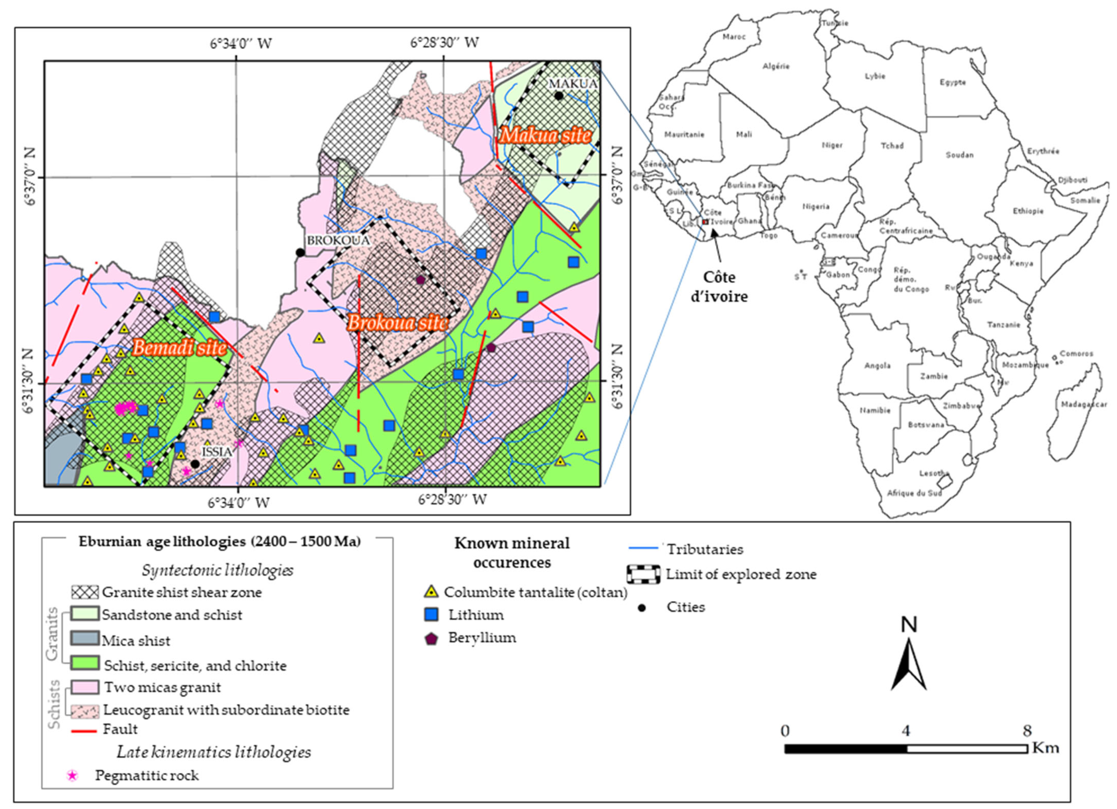
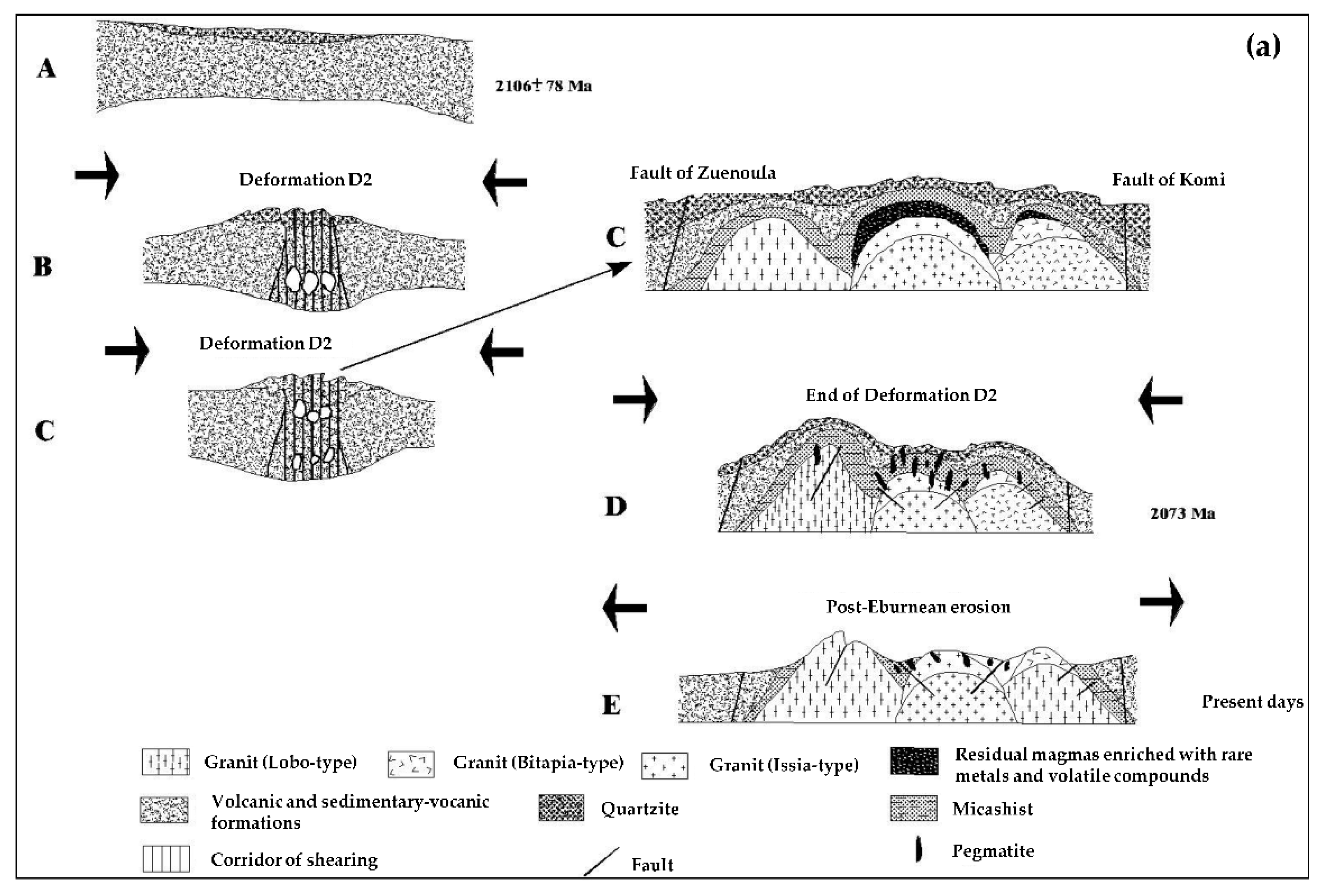
2.1. Study Area and Geology
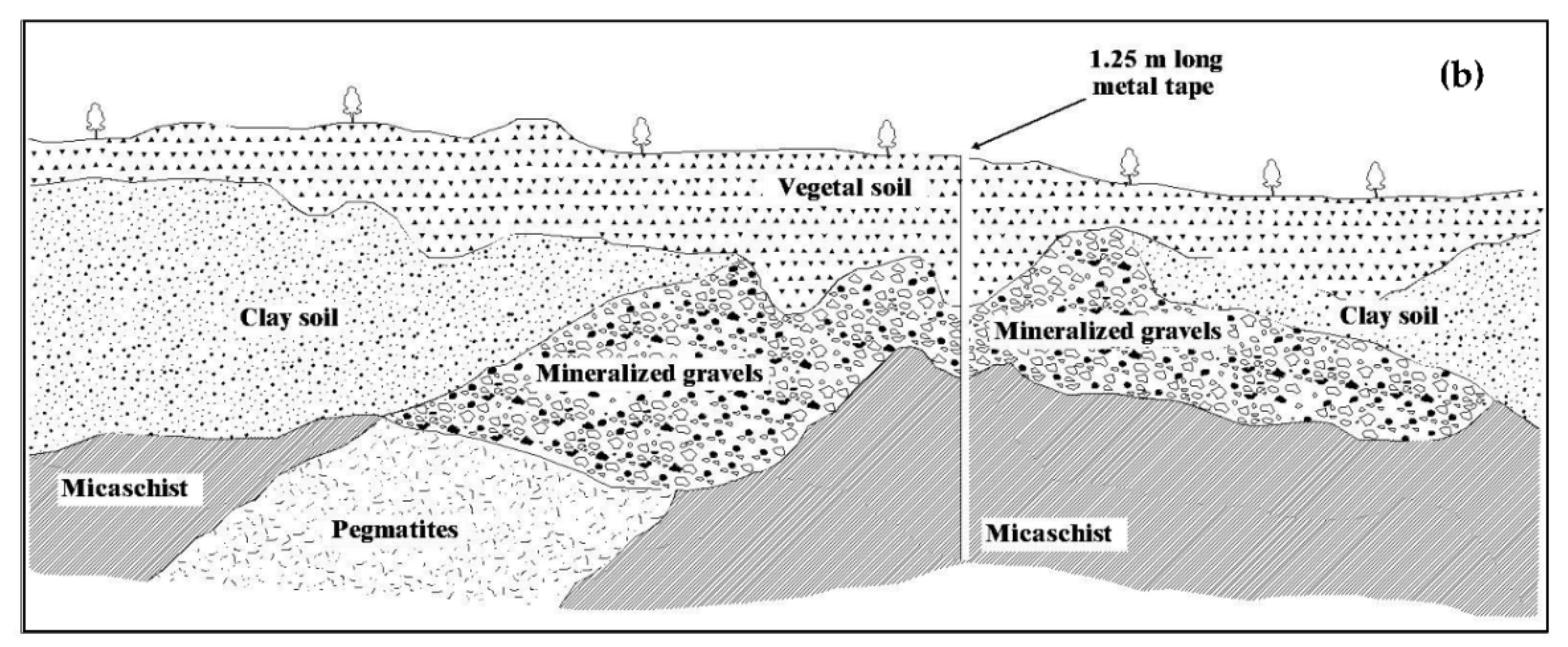
2.2. Mineralization System Analysis and Data Used
2.3. Data Used
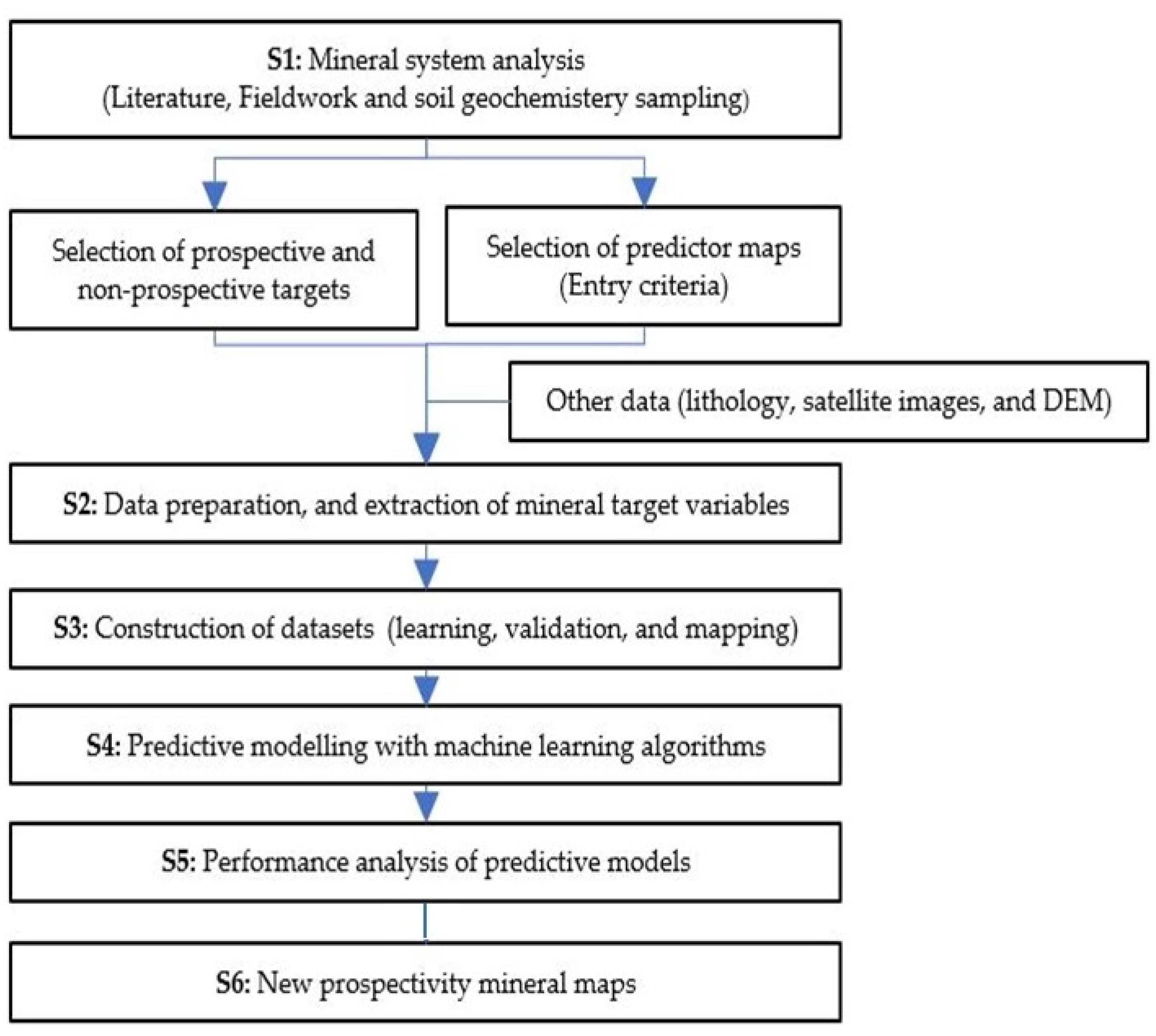
3. Methodology
3.1. Classification with SVM, KNN and RF Algorithms Machine-Learning
3.2. Selection and Extraction of Predictor Maps
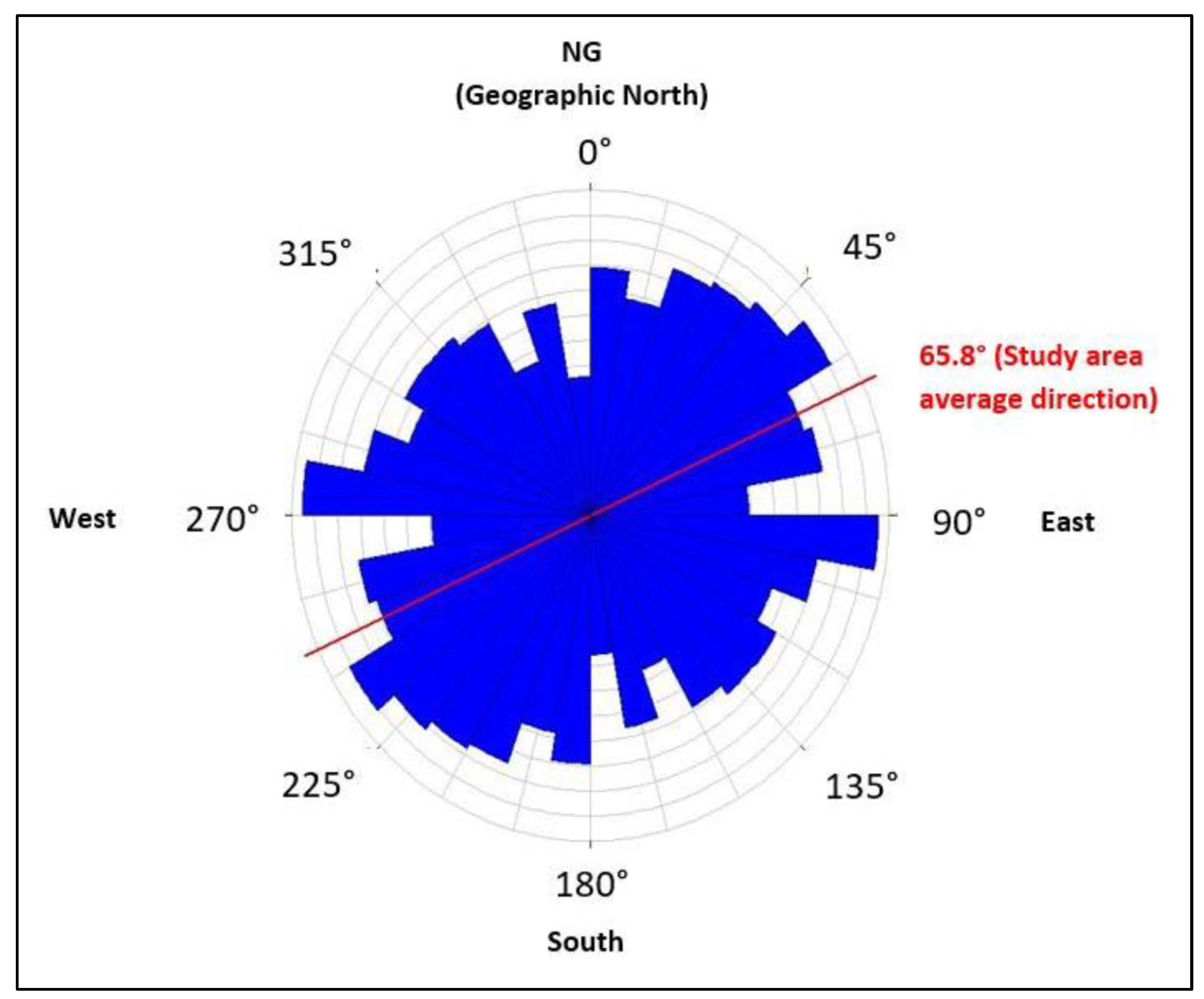
3.2.1. Extraction of Structural Evidence Map
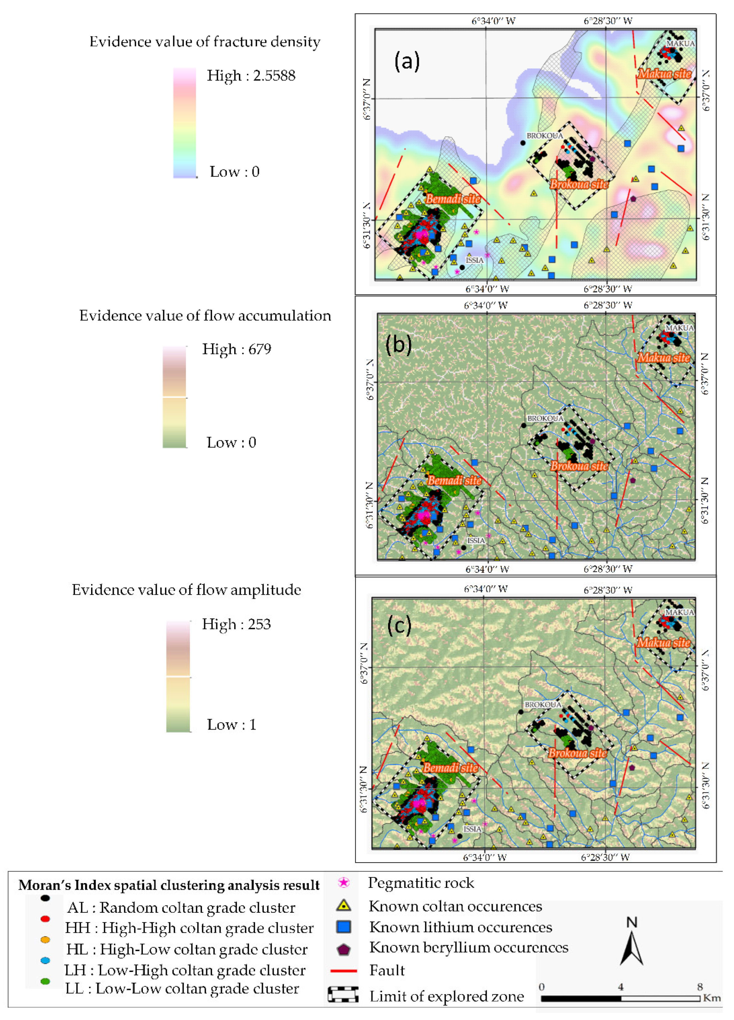
3.2.2. Extraction of Hydrological Evidence Criteria
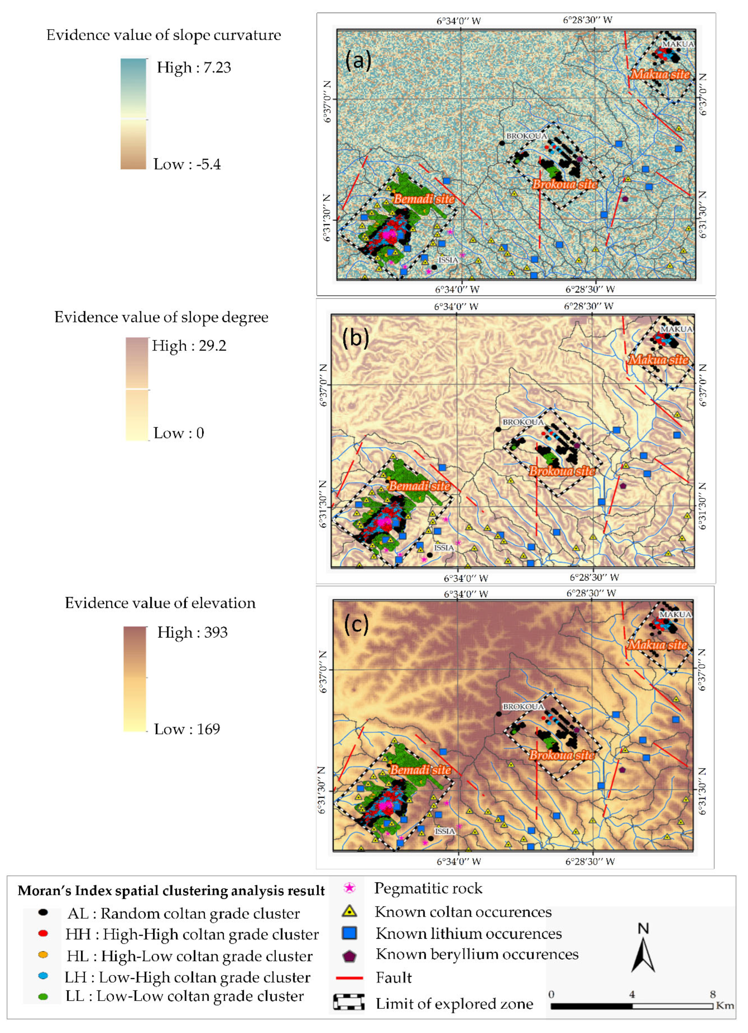
3.2.3. Extraction of Geomorphologic Evidence Criteria
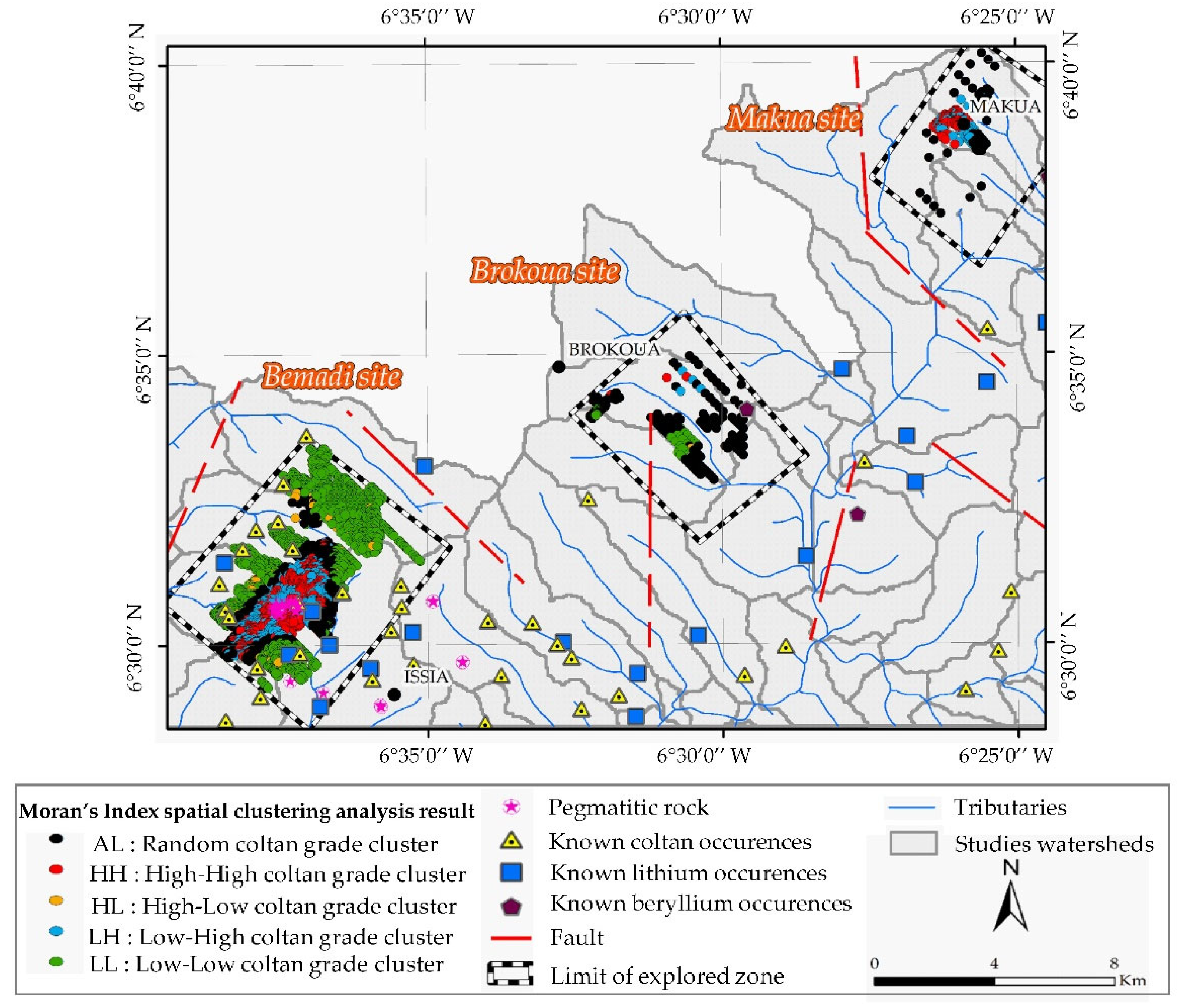
3.3. Selection and Extraction of Mineral Targets
3.4. Datasets and Processing
3.5. Evaluation of Predictive Models and Validation of Results
3.6. Prospectivity Mapping Process
4. Machine-Learning Algorithms Selection
5. Training of SVM and Other Models
6. Results
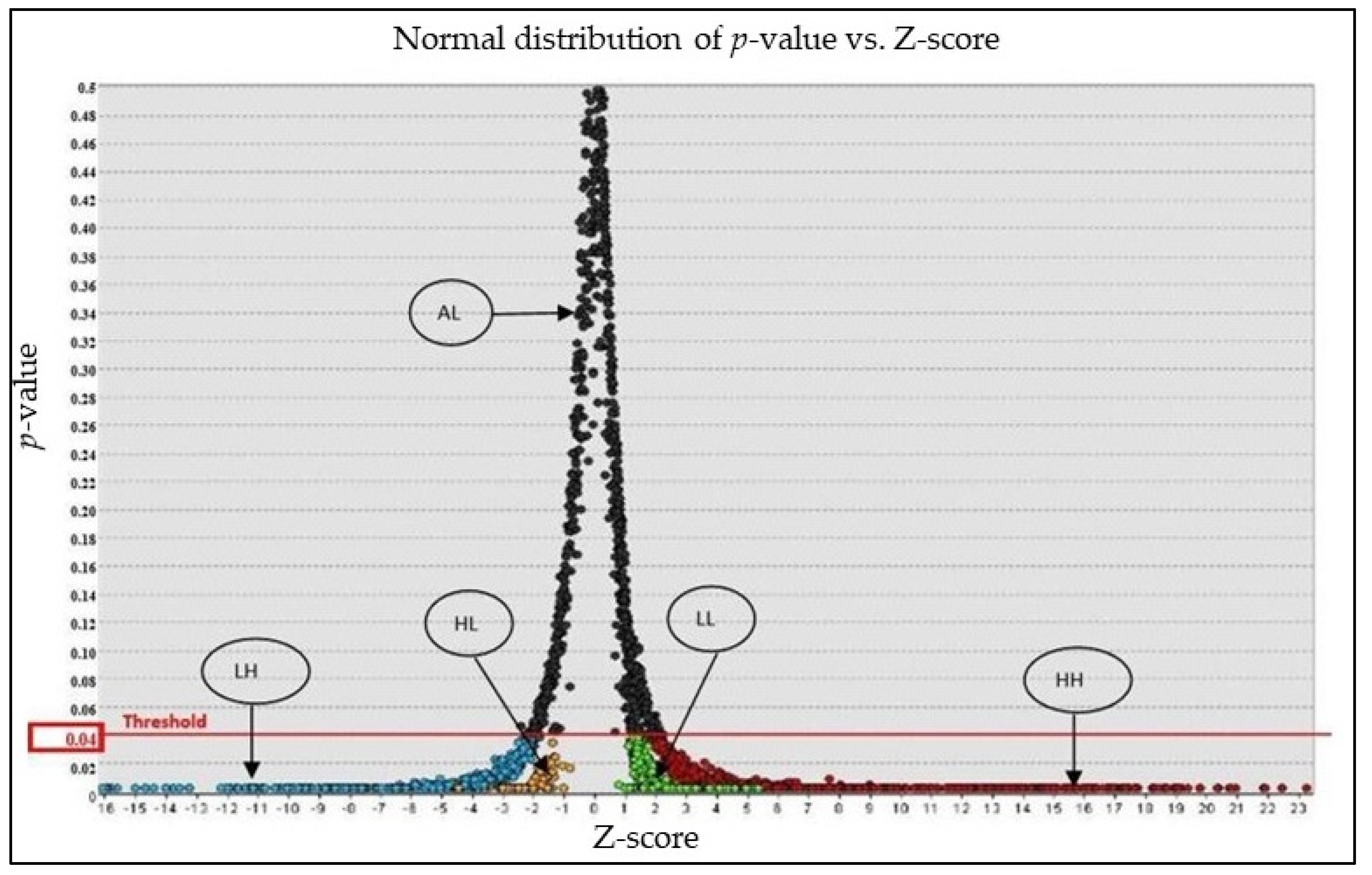
6.1. Discrimination of Mineral Targets
6.2. Machine-Learning Training Phases Analysis
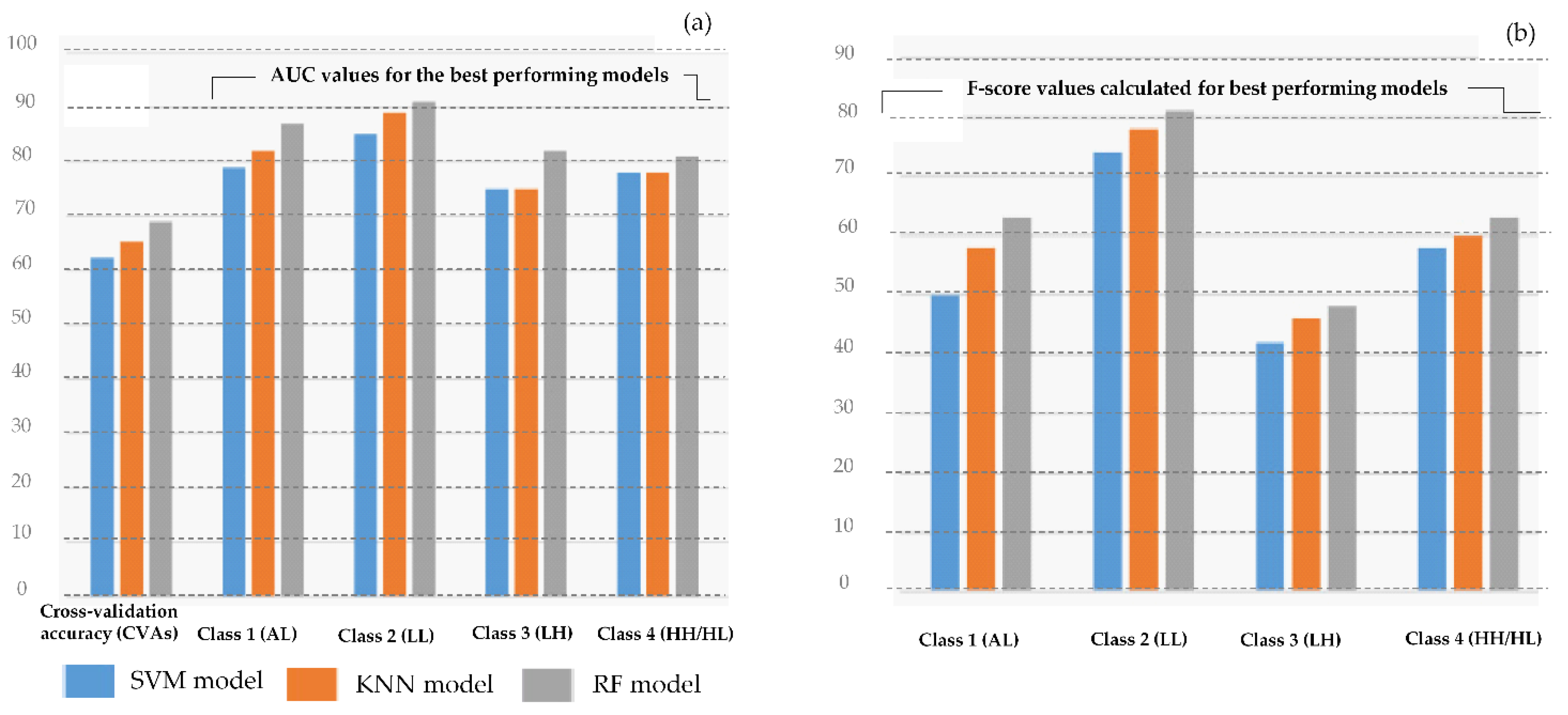
6.3. Evaluation of Robustness of Output Models
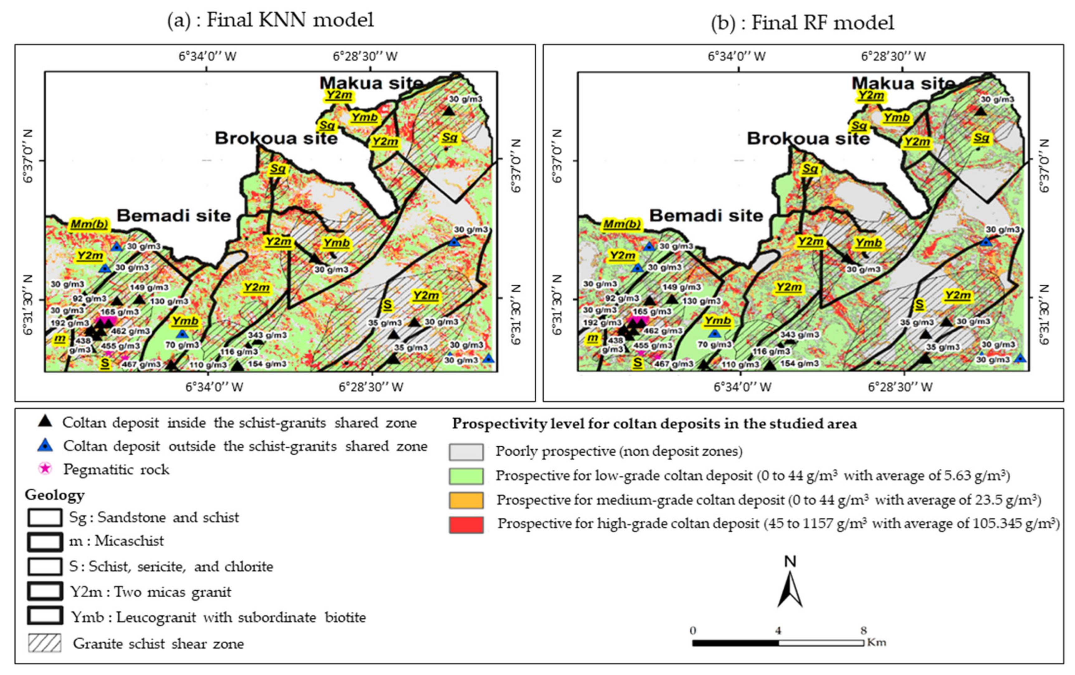
6.4. Evaluation of Sensitivity of the Prospectivity Maps Generated
7. Discussion
8. Conclusions
Author Contributions
Funding
Acknowledgments
Conflicts of Interest
References
- Rodriguez-Galiano, V.; Sanchez-Castillo, M.; Chica-Olmo, M.; Chica-Rivas, M. Machine learning predictive models for mineral prospectivity: An evaluation of neural networks, random forest, regression trees and support vector machines. Ore Geol. Rev. 2015, 71, 804–818. [Google Scholar] [CrossRef]
- Zuo, R.; et Carranza, E.J.M. Support vector machine: A tool for mapping mineral prospectivity. Comput. Geosci. Geocomputation Miner. Explor. Targets 2011, 37, 1967–1975. [Google Scholar] [CrossRef]
- Abedi, M.; Norouzi, G.-H. Integration of various geophysical data with geological and geochemical data to determine additional drilling for copper exploration. J. Appl. Geophys. 2012, 83, 35–45. [Google Scholar] [CrossRef]
- Yu, L.; Porwal, A.; Holden, E.-J.; Dentith, M.C. Towards automatic lithological classification from remote sensing data using support vector machines. Comput. Geosci. 2012, 45, 229–239. [Google Scholar] [CrossRef]
- Et Granek, J.; Haber, E. Data mining for real mining: A robust algorithm for prospectivity mapping with uncertainties. In Proceedings of the SIAM International Conference on Data Mining 2015, SDM 2015, Vancouver, BC, Canada, 30 April–2 May 2015; pp. 145–153. [Google Scholar] [CrossRef]
- Shabankareh, M.; Hezarkhani, A. Application of support vector machines for copper potential mapping in Kerman region, Iran. J. Afr. Earth Sci. 2017, 128, 116–126. [Google Scholar] [CrossRef]
- Nguyen, T.H.; Jones, S.; Soto-Berelov, M.; Haywood, A.; Hislop, S. A Comparison of Imputation Approaches for Estimating Forest Biomass Using Landsat Time-Series and Inventory Data. Remote Sens. 2018, 10, 1825. [Google Scholar] [CrossRef]
- Carranza, E.J.M.; Laborte, A.G. Random forest predictive modeling of mineral prospectivity with small number of prospects and data with missing values in Abra (Philippines). Comput. Geosci. 2015, 74, 60–70. [Google Scholar] [CrossRef]
- Carranza, E.J.M.; Laborte, A.G. Data-Driven Predictive Modeling of Mineral Prospectivity Using Random Forests: A Case Study in Catanduanes Island (Philippines). Nonrenewable Resour. 2015, 25, 35–50. [Google Scholar] [CrossRef]
- Hariharan, S.; Tirodkar, S.; Porwal, A.; Bhattacharya, A.; Joly, A. Random Forest-Based Prospectivity Modelling of Greenfield Terrains Using Sparse Deposit Data: An Example from the Tanami Region, Western Australia. Nonrenewable Resour. 2017, 26, 489–507. [Google Scholar] [CrossRef]
- Harris, J.R.; Grunsky, E.; Behnia, P.; Corrigan, D. Data-and knowledge-driven mineral prospectivity maps for Canada’s North. Ore Geol. Rev. 2015, 71, 788–803. [Google Scholar] [CrossRef]
- Parsa, M. A data augmentation approach to XGboost-based mineral potential mapping: An example of carbonate-hosted ZnPb mineral systems of Western Iran. J. Geochem. Explor. 2021, 228, 106811. [Google Scholar] [CrossRef]
- King, G.; Zeng, L.; Tomz, M. Logistic Regression in Rare Events Data. J. Stat. Softw. 2003, 8, 137–163. [Google Scholar] [CrossRef]
- Xiong, Y.; Zuo, R. GIS-based rare events logistic regression for mineral prospectivity mapping. Comput. Geosci. 2018, 111, 18–25. [Google Scholar] [CrossRef]
- Bolouki, S.M.; Ramazi, H.R.; Maghsoudi, A.; Beiranvand Pour, A.; Sohrabi, G. A Remote Sensing-Based Application of Bayesian Networks for Epithermal Gold Potential Mapping in Ahar-Arasbaran Area, NW Iran. Remote Sens. 2020, 12, 105. [Google Scholar] [CrossRef]
- Noack, S.; Knobloch, A.; Etzold, S.H.; Barth, A.; Kallmeier, E. Spatial predictive mapping using artificial neural networks. ISPRS Int. Arch. Photogramm. Remote Sens. Spat. Inf. Sci. 2014, XL-2, 79–86. [Google Scholar] [CrossRef]
- Zhao, J.; Chen, S.; et Zuo, R. Identifying geochemical anomalies associated with Au-Cu mineralization using multifractal and artificial neural network models in the Ningqiang district, Shaanxi, China. J. Geochem. Explor. 2016, 164, 54–64. [Google Scholar] [CrossRef]
- Chen, Y.; Lu, L.; Li, X. Application of continuous restricted Boltzmann machine to identify multivariate geochemical anomaly. J. Geochem. Explor. 2014, 140, 56–63. [Google Scholar] [CrossRef]
- Chen, Y. Mineral potential mapping with a restricted Boltzmann machine. Ore Geol. Rev. 2015, 71, 749–760. [Google Scholar] [CrossRef]
- Chen, G.; Huang, N.; Wu, G.; Luo, L.; Wang, D.; Cheng, Q. Mineral prospectivity mapping based on wavelet neural network and Monte Carlo simulations in the Nanling W-Sn metallogenic province. Ore Geol. Rev. 2022, 143, 104–765. [Google Scholar] [CrossRef]
- Parsa, M.; Carranza, E.J.M.; Ahmadi, B. Deep GMDH Neural Networks for Predictive Mapping of Mineral Prospectivity in Terrains Hosting Few but Large Mineral Deposits. Nonrenewable Resour. 2021, 31, 37–50. [Google Scholar] [CrossRef]
- Abedi, M.; Norouzi, G.-H.; Bahroudi, A. Support vector machine for multi-classification of mineral prospectivity areas. Comput. Geosci. 2012, 46, 272–283. [Google Scholar] [CrossRef]
- Asadi, H.H.; Porwal, A.; Fatehi, M.; Kianpouryan, S.; Lu, Y.-J. Exploration feature selection applied to hybrid data integration modeling: Targeting copper-gold potential in central Iran. Ore Geol. Rev. 2015, 71, 819–838. [Google Scholar] [CrossRef]
- Rombach, M. Rapport de Synthèse de la Minéralisation Alluvionnaire de la Région de SAIOUA (Issia); SODEMI: Abidjan, Côte d’Ivoire, 1960. [Google Scholar]
- Cruys, H. Prospection pour Columbo-Tantalite dans la Région d’Issia. Campagne Juillet 1963 Avril 1965; SODEMI: Abidjan, Côte d’Ivoire, 1965. [Google Scholar]
- Adam, H. Les Pegmatites de la Région d’Issia; SODEMI: Abidjan, Côte d’Ivoire, 1968. [Google Scholar]
- Papon, A.; Lemarchand, R. Geologie et Mineralisations du Sud-Ouest de la Cote-d’Ivoire; Synthèse des Travaux de l’Operation SASCA, 1962–1968; B.R.G.M.: Paris, France, 1973. [Google Scholar]
- Feybesse, J.-L.; Milési, J.P.; Ouédraogo, M.F.; Prost, A.E. La ceinture Protérozoique inférieur de Boromo-Goren (Burkina Faso): Un exemple d’inférence entre deux phases transcurrentes éburnéennes. C.R. Acad. Sci. 1990, 310, 1353–1360. [Google Scholar]
- Vidal, M.; Prost, A.E.; Aric, G.; Lemoine, S. Présence d’un socle antérieur à une suture océanique du Birimien inférieur en Côte d’Ivoire (afrique de l’Ouest). C.R. Acad. Sci. 1992, 2, 1085–1090. [Google Scholar]
- Allou, A.B. Facteurs, Paramètres, Dynamique de Distribution et Genèse des dépôts de Columbo-Tantalite d’Issia, Centre-Ouest de la Côte d’Ivoire; Université du Québec à Chicoutimi: Montréal, QC, Canada, 2005. [Google Scholar]
- Porwal, A.; González-Álvarez, I.; Markwitz, V.; McCuaig, T.; Mamuse, A. Weights-of-evidence and logistic regression modeling of magmatic nickel sulfide prospectivity in the Yilgarn Craton, Western Australia. Ore Geol. Rev. 2010, 38, 184–196. [Google Scholar] [CrossRef]
- Joly, A.; Porwal, A.; McCuaig, T.C. Exploration targeting for orogenic gold deposits in the Granites-Tanami Orogen: Mineral system analysis, targeting model and prospectivity analysis. Ore Geol. Rev. 2012, 48, 349–383. [Google Scholar] [CrossRef]
- Joly, A.; Porwal, A.; McCuaig, T.C.; Chudasama, B.; Dentith, M.C.; Aitken, A.R. Mineral systems approach applied to GIS-based 2D-prospectivity modelling of geological regions: Insights from Western Australia. Ore Geol. Rev. 2015, 71, 673–702. [Google Scholar] [CrossRef]
- Bonham-Carter, G.F.; Agterberg, F.P. Application of a Microcomputer-Based Geographic Information System to Mineral-Potential Mapping. Geological Survey of Canada Contribution Number 47488. In Microcomputer Applications in Geology 2; Computers and Geology; Hanley, J.T., Merriam, D.F., Eds.; Pergamon: Amsterdam, The Netherlands, 1990; pp. 49–74. [Google Scholar] [CrossRef]
- Carranza, E.; van Ruitenbeek, F.; Hecker, C.; van der Meijde, M.; van der Meer, F. Knowledge-guided data-driven evidential belief modeling of mineral prospectivity in Cabo de Gata, SE Spain. Int. J. Appl. Earth Obs. Geoinf. 2008, 10, 374–387. [Google Scholar] [CrossRef]
- Parsa, M.; Lentz, D.R.; Walker, J.A. Predictive Modeling of Prospectivity for VHMS Mineral Deposits, Northeastern Bathurst Mining Camp, NB, Canada, Using an Ensemble Regularization Technique. Nat. Resour. Res. 2022, 1–18. [Google Scholar] [CrossRef]
- Carranza, E.J.M. Geocomputation of mineral exploration targets. Comput. Geosci. 2011, 37, 1907–1916. [Google Scholar] [CrossRef]
- Porwal, A.; Carranza, E.J.M.; Hale, M. A Hybrid Neuro-Fuzzy Model for Mineral Potential Mapping. Math. Geol. 2004, 36, 803–826. [Google Scholar] [CrossRef]
- Yousefi, M.; Carranza, E.J.M. Fuzzification of continuous-value spatial evidence for mineral prospectivity mapping. Comput. Geosci. 2015, 74, 97–109. [Google Scholar] [CrossRef]
- Mccuaig, T.C. Sherlock, R.L. Exploration Targeting. Proc. Explor. 2017, 17, 75–82. [Google Scholar]
- Kottek, M.; Grieser, J.; Beck, C.; Rudolf, B.; Rubel, F. World map of the Köppen-Geiger climate classification updated. Meteorol. Z. 2006, 15, 259–263. [Google Scholar] [CrossRef]
- Sun, T.; Chen, F.; Zhong, L.; Liu, W.; Wang, Y. GIS-based mineral prospectivity mapping using machine learning methods: A case study from Tongling ore district, eastern China. Ore Geol. Rev. 2019, 109, 26–49. [Google Scholar] [CrossRef]
- Sheykhmousa, M.; Mahdianpari, M.; Ghanbari, H.; Mohammadimanesh, F.; Ghamisi, P.; Homayouni, S. Support Vector Machine Versus Random Forest for Remote Sensing Image Classification: A Meta-Analysis and Systematic Review. IEEE J. Sel. Top. Appl. Earth Obs. Remote Sens. 2020, 13, 6308–6325. [Google Scholar] [CrossRef]
- Breiman, L. Bagging predictors. Mach. Learn. 1996, 24, 123–140. [Google Scholar] [CrossRef]
- Belgiu, M.; Drăguţ, L. Random forest in remote sensing: A review of applications and future directions. ISPRS J. Photogramm. Remote Sens. 2016, 114, 24–31. [Google Scholar] [CrossRef]
- Breiman, L. Random forests. Mach. Learn. 2001, 45, 5–32. [Google Scholar] [CrossRef]
- Balabin, R.M.; Safieva, R.Z.; Lomakina, E.I. Near-infrared (NIR) spectroscopy for motor oil classification: From discriminant analysis to support vector machines. Microchem. J. 2011, 98, 121–128. [Google Scholar] [CrossRef]
- Walsh, S.J.; Mynar, F. Landsat digital enhancements for lineament detection. Environ. Earth Sci. 1986, 8, 123–128. [Google Scholar] [CrossRef]
- Paganelli, F.; Grunsky, E.C.; Richards, J.P.; Pryde, R. Use of RADARSAT-1 principal component imagery for structural mapping: A case study in the Buffalo Head Hills area, northern central Alberta, Canada. Can. J. Remote Sens. 2003, 29, 111–140. [Google Scholar] [CrossRef]
- Adiri, Z.; El Harti, A.; Jellouli, A.; Lhissou, R.; Maacha, L.; Azmi, M.; Zouhair, M.; Bachaoui, E.M. Comparison of Landsat-8, ASTER and Sentinel 1 satellite remote sensing data in automatic lineaments extraction: A case study of Sidi Flah-Bouskour inlier, Moroccan Anti Atlas. Adv. Space Res. 2017, 60, 2355–2367. [Google Scholar] [CrossRef]
- Corgne, S.; Magagi, R.; Yergeau, M.; Sylla, D. An integrated approach to hydro-geological lineament mapping of a semi-arid region of West Africa using Radarsat-1 and GIS. Remote Sens. Environ. 2010, 114, 1863–1875. [Google Scholar] [CrossRef]
- Hashim, M.; Ahmad, S.; Md Johari, M.A.; Pour, A.B. Automatic lineament extraction in a heavily vegetated region using Landsat Enhanced Thematic Mapper (ETM+) imagery. Adv. Space Res. 2013, 51, 874–890. [Google Scholar] [CrossRef]
- Robson, R. A multi-component rose diagram. J. Struct. Geol. 1994, 16, 1039–1040. [Google Scholar] [CrossRef]
- Triboulet, C.; et Feybesse, J.-L. Les métabasites birimiennes et archéennes de la région de Toulepleu-Ity (Côte-d’lvoire): Des roches portées à 8 kbar (≈24 km) et 14 kbar (≈42 km) au Paléoprotérozoïque. Comptes Rendus De L’académie Des Sci.-Ser. IIA-Earth Planet. Sci. 1998, 327, 61–66. [Google Scholar] [CrossRef]
- Koudou, A.; Kouamé, F.K.; Youan Ta, M.; Saley, M.B.; Jourda, J.P. Contribution des données ETM+ de Landsat, de l’analyse multicritère et d’un SIG à l’identification de secteurs à potentialité aquifère en zone de socle du bassin versant du N’zi (Côte d’Ivoire). GéoProdig, portail d’information géographique. Available online: http://geoprodig.cnrs.fr/items/show/48174 (accessed on 16 February 2022).
- Koudou, A.; Assoma, T.V.; Adiaffi, B.; Ta, M.Y.; Kouame, K.F.; et Lasm, T. Analyses Statistique et Geostatistique de la Fracturation extraite de l’imagerie Asar Envisat du Sud- est de la Côte D’Ivoire. Larhyss J. 2014, 11, 147–166. [Google Scholar]
- Nkono, C.; Féménias, O.; Lesne, A.; Mercier, J.-C.; Demaiffe, D. Fractal Analysis of Lineaments in Equatorial Africa: Insights on Lithospheric Structure. Open J. Geol. 2013, 3, 157–168. [Google Scholar] [CrossRef]
- Saadi, N.; Zaher, M.A.; El-Baz, F.; Watanabe, K. Integrated remote sensing data utilization for investigating structural and tectonic history of the Ghadames Basin, Libya. Int. J. Appl. Earth Obs. Geoinformation 2011, 13, 778–791. [Google Scholar] [CrossRef]
- Moran, P.A.P. Notes on continuous stochastic phenomena. Biometrika 1950, 37, 17–23. [Google Scholar] [CrossRef] [PubMed]
- Anselin, L. The Local Indicators of Spatial Association—LISA. Geogr. Anal. 1995, 27, 93–115. [Google Scholar] [CrossRef]
- Peters, J.; De Baets, B.; Verhoest, N.E.C.; Samson, R.; Degroeve, S.; De Becker, P.; Huybrechts, W. Random forests as a tool for ecohydrological distribution modelling. Ecol. Model. 2007, 207, 304–318. [Google Scholar] [CrossRef]
- Toth, R.; Ribault, J.; Gentile, J.; Sperling, D.; Madabhushi, A. Simultaneous segmentation of prostatic zones using Active Appearance Models with multiple coupled levelsets. Comput. Vis. Image Underst. 2013, 117, 1051–1060. [Google Scholar] [CrossRef] [PubMed]
- Chen, Y.; Wu, W. Mapping mineral prospectivity using an extreme learning machine regression. Ore Geol. Rev. 2017, 80, 200–213. [Google Scholar] [CrossRef]
- Bui, D.T.; Tuan, T.A.; Klempe, H.; Pradhan, B.; Revhaug, I. Spatial prediction models for shallow landslide hazards: A comparative assessment of the efficacy of support vector machines, artificial neural networks, kernel logistic regression, and logistic model tree. Landslides 2015, 13, 361–378. [Google Scholar] [CrossRef]
- Nykänen, V.; Lahti, I.; Niiranen, T.; Korhonen, K. Receiver operating characteristics (ROC) as validation tool for prospectivity models—A magmatic Ni–Cu case study from the Central Lapland Greenstone Belt, Northern Finland. Ore Geol. Rev. 2015, 71, 853–860. [Google Scholar] [CrossRef]
- Zuo, R. Selection of an elemental association related to mineralization using spatial analysis. J. Geochem. Explor. 2018, 184, 150–157. [Google Scholar] [CrossRef]
- Chen, Y.; An, A. Application of ant colony algorithm to geochemical anomaly detection. J. Geochem. Explor. 2016, 164, 75–85. [Google Scholar] [CrossRef]
- Bonham-Carter, G.F.; Bonham-Carter, G. Geographic Information Systems for Geoscientists: Modelling with GIS (No. 13); Elsevier: Amsterdam, The Netherlands, 1994. [Google Scholar]
- Yousefi, M.; Carranza, E.J.M. Prediction–area (P–A) plot and C–A fractal analysis to classify and evaluate evidential maps for mineral prospectivity modeling. Comput. Geosci. 2015, 79, 69–81. [Google Scholar] [CrossRef]
- Yousefi, M.; Carranza, E.J.M. Data-Driven Index Overlay and Boolean Logic Mineral Prospectivity Modeling in Greenfields Exploration. Nonrenewable Resour. 2015, 25, 3–18. [Google Scholar] [CrossRef]
- Yousefi, M.; Carranza, E.J.M. Geometric average of spatial evidence data layers: A GIS-based multi-criteria decision-making approach to mineral prospectivity mapping. Comput. Geosci. 2015, 83, 72–79. [Google Scholar] [CrossRef]
- Du, X.; Zhou, K.; Cui, Y.; Wang, J.; Zhang, N.; Sun, W. Application of fuzzy analytical hierarchy process (AHP) and prediction-area (P-A) plot for mineral prospectivity mapping: A case study from the Dananhu metallogenic belt, Xinjiang, NW China. Arab. J. Geosci. 2016, 9, 298. [Google Scholar] [CrossRef]
- Gao, Y.; Zhang, Z.; Xiong, Y.; Zuo, R. Mapping mineral prospectivity for Cu polymetallic mineralization in southwest Fujian Province, China. Ore Geol. Rev. 2016, 75, 16–28. [Google Scholar] [CrossRef]
- Nezhad, S.G.; Mokhtari, A.R.; Rodsari, P.R. The true sample catchment basin approach in the analysis of stream sediment geochemical data. Ore Geol. Rev. 2017, 83, 127–134. [Google Scholar] [CrossRef]
- Zhang, N.; Zhou, K.; Du, X. Application of fuzzy logic and fuzzy AHP to mineral prospectivity mapping of porphyry and hydrothermal vein copper deposits in the Dananhu-Tousuquan island arc, Xinjiang, NW China. J. Afr. Earth Sci. 2017, 128, 84–96. [Google Scholar] [CrossRef]
- Almasi, A.; Yousefi, M.; Carranza, E.J.M. Prospectivity analysis of orogenic gold deposits in Saqez-Sardasht Goldfield, Zagros Orogen, Iran. Ore Geol. Rev. 2017, 91, 1066–1080. [Google Scholar] [CrossRef]
- Roshanravan, B.; Aghajani, H.; Yousefi, M.; Kreuzer, O. Particle Swarm Optimization Algorithm for Neuro-Fuzzy Prospectivity Analysis Using Continuously Weighted Spatial Exploration Data. Nonrenewable Resour. 2018, 28, 309–325. [Google Scholar] [CrossRef]
- Roshanravan, B.; Aghajani, H.; Yousefi, M.; Kreuzer, O. An Improved Prediction-Area Plot for Prospectivity Analysis of Mineral Deposits. Nonrenewable Resour. 2018, 28, 1089–1105. [Google Scholar] [CrossRef]
- Bater, C.W.; et Coops, N.C. Evaluating error associated with lidar-derived DEM interpolation. Comput. Geosci. 2009, 35, 289–300. [Google Scholar] [CrossRef]
- Silverman, B.W.; Jones, M.C.; Fix, E.; Hodges, J.L. An Important Contribution to Nonparametric Discriminant Analysis and Density Estimation: Commentary on Fix and Hodges (1951). Int. Stat. Rev. 1989, 57, 233. [Google Scholar] [CrossRef]
- Joseph Santarcangelo (2022). Data Normalization and Standardization. MATLAB Central File Exchange. Available online: https://www.mathworks.com/matlabcentral/fileexchange/48677-data-normalization-and-standardization (accessed on 9 November 2022).
- Landis, J.R.; Koch, G.G. The Measurement of Observer Agreement for Categorical Data. Biometrics 1977, 33, 159–174. [Google Scholar] [CrossRef] [PubMed]
- Japkowicz, N.; Stephen, S. The class imbalance problem: A systematic study1. Intell. Data Anal. 2002, 6, 429–449. [Google Scholar] [CrossRef]
- Chawla, N.V.; Lazarevic, A.; Hall, L.O.; Bowyer, K.W. SMOTE Boost: Improving Prediction of the Minority Class in Boosting. In Proceedings of the European Conference on Principles of Data Mining and Knowledge Discovery, Cavtat-Dubrovnik, Croatia, 22–26 September 2003; pp. 107–119. [Google Scholar] [CrossRef]
- Galar, M.; Fernandez, A.; Barrenechea, E.; Bustince, H.; Herrera, F. A Review on Ensembles for the Class Imbalance Problem: Bagging-, Boosting-, and Hybrid-Based Approaches. IEEE Trans. Syst. Man Cybern. Part C Appl. Rev. 2012, 42, 463–484. [Google Scholar] [CrossRef]
- Li, T.; Xia, Q.; Zhao, M.; Gui, Z.; Leng, S. Prospectivity Mapping for Tungsten Polymetallic Mineral Resources, Nanling Metallogenic Belt, South China: Use of Random Forest Algorithm from a Perspective of Data Imbalance. Nonrenewable Resour. 2019, 29, 203–227. [Google Scholar] [CrossRef]
- Xiong, Y.; Zuo, R. Recognizing multivariate geochemical anomalies for mineral exploration by combining deep learning and one-class support vector machine. Comput. Geosci. 2020, 140, 104484. [Google Scholar] [CrossRef]
- Alyasin, E.I.; Ata, O.; Mohammedqasim, H. Novel hybrid classification model for multi-class imbalanced lithology dataset. Optik 2022, 270, 170047. [Google Scholar] [CrossRef]
- Lui, T.C.; Gregory, D.D.; Anderson, M.; Lee, W.-S.; Cowling, S.A. Applying machine learning methods to predict geology using soil sample geochemistry. Appl. Comput. Geosci. 2022, 16, 100094. [Google Scholar] [CrossRef]
- da Silva, G.F.; Silva, A.M.; Toledo, C.L.B.; Junior, F.C.; Klein, E.L. Predicting mineralization and targeting exploration criteria based on machine-learning in the Serra de Jacobina quartz-pebble-metaconglomerate Au-(U) deposits, São Francisco Craton, Brazil. J. South Am. Earth Sci. 2022, 116, 103815. [Google Scholar] [CrossRef]
- Jacob, R.J.; Bluck, B.J.; Ward, J.D. Tertiary-age diamondiferous fluvial deposits of the lower orange river valley, southwestern Africa. Econ. Geol. 1999, 94, 749–755. [Google Scholar] [CrossRef]


| Nature | Format | Source | Spatial Resolution | Spectral Resolution | Study Parameters | Usages |
|---|---|---|---|---|---|---|
| Mineralogy | Vector (points) | Fieldwork | 25 m × 50 m | Concentrated Nb-Ta content in gravels. | Identification of mineral targets. | |
| Hydrology | Matrix | ASTER (ASTGTM2_N06 W007_dem) of 17 October 2011. | 30 m | Surface accumulation of runoff, flow amplitude (or magnitude and direction). | Identification of areas suitable for sediment transport and deposition. | |
| Morphology | Matrix | ASTER (ASTGTM2_N06 W007_dem) of 17 October 2011. | 30 m | Degree of slope inclination, profile and curvature of slope and, relief. | Identification of natural trap areas (favorable for erosion and deposition). | |
| Structural | Matrix | Sentinel 2B MSI, level 1C, Date 24 December 2017 | 10, 20, 60 m | 13 bands between 443 and 2190 nm | Discontinuity In pixels | Extraction of lineaments |
| Sentinel 1A SAR (VV & HH), Date 6 January 2018 | 40 m | Band C | ||||
| ESRI world imagery (Maxar, Geoeye, Earthstar Geographics, CNES/Airbus DS, USDA, USGS, AeroGRID, IGN and, the GIS USER community) | 15 m | Actual appearance of objects | Validation of faults and fractures. | |||
| SPOT-5 | 2.5–10 m | 5 bands between 0.5 and 0.89 µm | Actual appearance of objects | |||
| Geology | Vector | Geological map (Government of Côte d’Ivoire) | 1:200,000 | Lithological surfaces, Pegmatite emplacements, Faults, Fractures | Understanding the geological context |
| N° | Evidence Layer Selected as Entry Criteria | Predictive Parameters Selected to Build the Machine-Learning Prediction Model |
|---|---|---|
| 1 | Evidence map of fracture density (Figure 5a). | Value of the fracture density extracted at the sample locations into deposits (clusters HH/HL, LL and LH) and non-deposit (cluster AL) targets. |
| 2 | Evidence map of flow accumulation area (Figure 5b). | Value of the flow accumulation surface extracted at the sample locations into deposits (clusters HH/HL, LL and LH) and non-deposit (cluster AL) targets. |
| 3 | Evidence map of flow accumulation or magnitude areas (Figure 5c). | Value of the flow magnitude extracted at the sample locations into deposits (clusters HH/HL, LL and LH) and non-deposit (cluster AL) targets. |
| 4 | Evidence map of slope curvature (Figure 6a). | Value of the slope curvature extracted at the sample locations into deposits (clusters HH/HL, LL and LH) and non-deposit (cluster AL) targets. |
| 5 | Evidence map of slope degree (Figure 6b). | Value of the slope inclination extracted at the sample locations into deposits (clusters HH/HL, LL and LH) and non-deposit (cluster AL) targets. |
| 6 | Evidence map of relief (Figure 6c). | Value of the elevation extracted at the sample locations into deposits (clusters HH/HL, LL and LH) and non-deposit (cluster AL) targets. |
| Learning Hyperparameters to Train SVM Machine-Learning Algorithms | |||||
|---|---|---|---|---|---|
| Two multi-class classification strategies tested: One-vs.-All (OvA) and One-vs.-One (OvO) | |||||
| Value of the box constraint level parameter used: 1 | |||||
| Model Category | Type of Output Model | Detection Function Parameter | Value of Detection Parameter | Kernel Scale Parameter | Value of Kernel Scale Parameter |
| SVM | Linear SVM | Linear | 1 | - | - |
| Quadratic Core SVM | Quadratic | 1 | - | - | |
| Cubic Core SVM | Cubic | 1 | - | - | |
| Fine Gaussian Kernel SVM | Gaussian | 0 | Fine | 61 | |
| Medium Gaussian Kernel SVM | Gaussian | 2 | Medium | 4 | |
| Coarse Gaussian Core SVM | Gaussian | 9 | Coarse | 8 | |
| Learning Parameters Used to Train KNN Machine-Learning Algorithms | |||||
| Separation Parameter | Number of Neighbors | Metric Distance Parameter | Weighting Parameter | ||
| KNN | Fine KNN | Fine | 1 | - | - |
| Median KNN | Medium | 10 | - | - | |
| Coarse KNN | Coarse | 100 | Coarse | - | |
| Cosine KNN | Medium | 10 | Cosine | - | |
| Cubic KNN | Medium | 10 | Cubic (Minkowski) | - | |
| Equal-weighted KNN | 1 | Weighted | Equal | ||
| Euclidean-weighted KNN | 10 | Weighted | Euclidean | ||
| Inverse distance weighted KNN | 100 | Weighted | Inverse distance | ||
| Inverse squared distance weighted KNN | - | 100 | Weighted | Inverse square distance | |
| Learning Hyperparameters Used to Train RF Machine-Learning Algorithms | |||||
| Assembly method used: Bagging trees; range of maximum number of splits tested: 10, 20 and 30; range of numbers of learners tested: 30–60–100 and 500; learning rate values used: 0.1 and 1; sub-space dimension value used: 1 | |||||
| Random Forest | RF-10 splits and 30 learners | RF-20 splits and 60 learners | |||
| RF-10 splits and 60 learners | RF-20 splits and 100 learners | ||||
| RF-10 splits and 500 learners | RF-20 splits and 500 learners | ||||
| RF-30 splits and 500 learners | RF-30 splits and 500 learners | ||||
| RF-30 splits and 100 learners | RF-30 splits and 60 learners | ||||
| RF-10 splits and 100 learners | RF-30 splits and 30 learners | ||||
| RF-20 splits and 30 learners | - | ||||
| CO Type | Number of Points | Nb-Ta Grade Range (g/m3) | Spatial Cluster/Outlier Nb-Ta Grade (g/m3) | Min/Max Moran’s I Index | Min/Max p-Value | Min/Max Number of Neighbors |
|---|---|---|---|---|---|---|
| HH | 767 | 45 to 1157 | 136.61 | 0.0005/14.35 | 0.002/0.038 | 7/554 |
| HL | 98 | 45 to 821 | 74.08 | −1.65/0 | 0.002/0.034 | 33/442 |
| LH | 513 | 0 to44 | 23.5 | −059/0 | 0.002/0.038 | 9/546 |
| LL | 1542 | 0 to 44 | 5.63 | 0/0.43 | 0.002/0.038 | 13/459 |
| AL | 789 | 0 to 1126 | 40.98 | −0.08/2.34 | 0.04/0.498 | 1/545 |
| Total | 3709 | - | - | - | - | - |
| Name of Model | Multi-Class Classification Strategy Used | Value of Detection Parameter | Value of Kernel Scale Parameter | CVA (%) | AUC Value (%) | |||
|---|---|---|---|---|---|---|---|---|
| Class1 (AL) | Class 2 (LL) | Class 3 (LH) | Class 4 (HH/HL) | |||||
| Linear kernel SVM | One vs. One | 1 | - | 41.6 | 63 | 58 | 51 | 55 |
| One vs. All | 1 | - | 39.8 | 58 | 63 | 58 | 54 | |
| Quadratic kernel SVM | One vs. One | 1 | - | 45.2 | 67 | 66 | 62 | 66 |
| One vs. All | 1 | - | 42 | 55 | 67 | 63 | 60 | |
| Cubic kernel SVM | One vs. One | 1 | - | 52 | 71 | 74 | 70 | 71 |
| One vs. All | 1 | - | 41.8 | 65 | 64 | 63 | 66 | |
| Fine Gaussian kernel SVM | One vs. One | 0 | 61 | 61.9 | 79 | 85 | 75 | 78 |
| One vs. All | 0 | 61 | 62.4 | 79 | 85 | 75 | 78 | |
| Medium Gaussian kernel SVM | One vs. One | 2 | 4 | 50.5 | 70 | 73 | 65 | 69 |
| One vs. All | 2 | 4 | 49.9 | 63 | 74 | 68 | 68 | |
| Coarse Gaussian kernel SVM | One vs. One | 9 | 8 | 41.7 | 65 | 65 | 59 | 58 |
| One vs. All | 9 | 8 | 42.7 | 59 | 65 | 59 | 56 | |
| Name of Model | Metric Distance Type | Distance Weighting Type | Number of Neighbors | CVA (%) | AUC Value (%) | |||
|---|---|---|---|---|---|---|---|---|
| Class 1 (AL) | Class 2 (LL) | Class 3 (LH) | Class 4 (HH/HL) | |||||
| Fine KNN | Euclidean | Equal | 1 | 63.7 | 73 | 81 | 67 | 73 |
| Cubic | Equal | 1 | 63.1 | 73 | 80 | 66 | 73 | |
| Cosine | Equal | 1 | 62.9 | 73 | 80 | 67 | 72 | |
| Medium KNN | Euclidean | Equal | 10 | 50.5 | 71 | 76 | 69 | 72 |
| Cubic | Equal | 10 | 49.7 | 71 | 75 | 69 | 72 | |
| Cosine | Equal | 10 | 49.1 | 70 | 75 | 69 | 73 | |
| Coarse KNN | Euclidean | Equal | 100 | 45.9 | 66 | 67 | 64 | 64 |
| Cubic | Equal | 100 | 45.8 | 65 | 66 | 64 | 64 | |
| Cosine | Equal | 100 | 45.9 | 65 | 67 | 63 | 64 | |
| Cosine KNN | Euclidean | Equal | 10 | 50.5 | 71 | 76 | 69 | 72 |
| Cosine | Equal | 10 | 49.1 | 70 | 75 | 69 | 73 | |
| Cubic KNN | Euclidean | Equal | 10 | 50.5 | 71 | 76 | 69 | 72 |
| Cubic | Equal | 10 | 49.7 | 71 | 75 | 69 | 72 | |
| Weighted- Euclidean KNN | Euclidean | Equal | 10 | 50.5 | 71 | 76 | 69 | 72 |
| IDW-weighted KNN | Euclidean | Inverse distance | 10 | 65.3 | 82 | 89 | 75 | 78 |
| IDW2-weighted KNN | Euclidean | Inverse distance- squared | 10 | 65.3 | 82 | 89 | 75 | 78 |
| Name of Model | Maximum Division | Number of Learners | Learning Rate | CVA (%) | AUC Value (%) | |||
|---|---|---|---|---|---|---|---|---|
| Class1 (AL) | Class 2 (LL) | Class 3 (LH) | Class 4 (HH/HL) | |||||
| RF (10sp/30L) | 10 | 30 | 0.1 | 67.3 | 87 | 91 | 80 | 81 |
| RF (10sp/60L) | 10 | 60 | 0.1 | 68.2 | 87 | 91 | 81 | 80 |
| RF (10sp/100L) | 10 | 100 | 0.1 | 68.3 | 87 | 91 | 81 | 81 |
| RF (10sp/500L) | 10 | 500 | 0.1 | 68.4 | 88 | 91 | 82 | 81 |
| RF (20sp/30L) | 20 | 30 | 0.1 | 67.2 | 86 | 90 | 80 | 80 |
| RF (20sp/60L) | 20 | 60 | 0.1 | 67,5 | 87 | 91 | 80 | 81 |
| RF (20sp/100L) | 20 | 100 | 0.1 | 68.3 | 87 | 91 | 81 | 81 |
| RF (20sp/500L) | 20 | 500 | 0.1 | 68.4 | 88 | 91 | 81 | 81 |
| RF (30sp/30L) | 30 | 30 | 0.1 | 67.3 | 86 | 90 | 80 | 80 |
| RF (30sp/60L) | 30 | 60 | 0.1 | 68.1 | 87 | 91 | 81 | 81 |
| RF (30sp/100L) | 30 | 100 | 0.1 | 69 | 87 | 91 | 82 | 81 |
| RF (30sp/500L) | 30 | 500 | 0.1 | 68.5 | 87 | 91 | 81 | 81 |
| Fine Gaussian Kernel SVM Confusion Matrix (Values are in %) | ||||
|---|---|---|---|---|
| Class 1 (AL) | Class 2 (LL) | Class 3 (LH) | Class 4 (HH/HL) | |
| Class 1 (AL) | 48.84 | 34.88 | 2.91 | 13.37 |
| Class 2 (LL) | 6.82 | 86.04 | 1.30 | 5.84 |
| Class 3 (LH) | 10.00 | 34.44 | 23.33 | 32.22 |
| Class 4 (HH/HL) | 5.23 | 25.00 | 11.63 | 58.14 |
| Number of samples for validation = 742; CVA = 63.34%; Kappa Coefficient = 0.46 | ||||
| IDW-weighted KNN Confusion matrix (values are in %) | ||||
| Class 1 (AL) | Class 2 (LL) | Class 3 (LH) | Class 4 (HH/HL) | |
| Class 1 (AL) | 60.47 | 20.93 | 9.3 | 9.3 |
| Class 2 (LL) | 7.14 | 83.12 | 1.62 | 8.12 |
| Class 3 (LH) | 12.22 | 16.67 | 38.89 | 32.22 |
| Class 4 (HH/HL) | 4.65 | 12.79 | 19.19 | 63.37 |
| Number of samples for validation = 742; CVA = 67.92%; Kappa Coefficient= 0.54 | ||||
| RF (30sp/100L) Confusion matrix (values are in %) | ||||
| Class 1 (AL) | Class 2 (LL) | Class 3 (LH) | Class 4 (HH/HL) | |
| Class 1 (AL) | 63.37 | 23.26 | 5.23 | 8.14 |
| Class 2 (LL) | 6.82 | 86.04 | 1.30 | 5.84 |
| Class 3 (LH) | 10.00 | 20.00 | 36.67 | 33.33 |
| Class 4 (HH/HL) | 5.23 | 16.86 | 15.12 | 62.79 |
| Number of samples for validation = 742; CVA = 69.41%; Kappa Coefficient = 0.56 | ||||
| Confusion Matrix of the RF Model Prospectivity MAP (Occupied Area) | ||||||
| Value is km2 | Predicted value from RF model prospectivity map | Total | ||||
| AL | LL | LH | HH/HL | |||
| Known Deposit value | AL | 0.80 | 0.40 | 0.09 | 0.12 | 1.40 |
| LL | 0.22 | 2.62 | 0.07 | 0.21 | 3.12 | |
| LH | 0.13 | 0.21 | 0.34 | 0.23 | 0.91 | |
| HH/HL | 0.16 | 0.48 | 0.25 | 0.91 | 1.80 | |
| Total | 1.31 | 3.71 | 0.75 | 1.47 | 7.23 | |
| Confusion Matrix of the KNN Model Prospectivity MAP (Occupied Area) | ||||||
| Value is km2 | Predicted value from KNN model prospectivity map | Total | ||||
| AL | LL | LH | HH/HL | |||
| Known Deposit value | AL | 0.70 | 0.41 | 0.12 | 0.17 | 1.40 |
| LL | 0.26 | 2.40 | 0.10 | 0.36 | 3.12 | |
| LH | 0.15 | 0.20 | 0.30 | 0.25 | 0.90 | |
| HH/HL | 0.20 | 0.45 | 0.24 | 0.92 | 1.81 | |
| Total | 1.31 | 3.46 | 0.76 | 1.70 | 7.23 | |
| Metrics of the RF prospectivity map (value is in percent) | ||||||
| Deposit type | Accuracy | Sensitivity | Specificity | F-score | ||
| AL | 61.07 | 57.06 | 91.25 | 59.00 | ||
| LL | 70.62 | 83.97 | 73.49 | 76.72 | ||
| LH | 45.52 | 37.36 | 93.56 | 41.04 | ||
| HH/HL | 62.12 | 50.56 | 89.78 | 55.74 | ||
| Metrics of the KNN prospectivity map (value is in percent) | ||||||
| Deposit type | Accuracy | Sensitivity | Specificity | F-score | ||
| AL | 53.44 | 50.00 | 89.54 | 51.66 | ||
| LL | 69.28 | 77.02 | 74.14 | 72.95 | ||
| LH | 39.68 | 33.19 | 92.79 | 36.14 | ||
| HH/HL | 54.12 | 50.83 | 85.61 | 52.42 | ||
Publisher’s Note: MDPI stays neutral with regard to jurisdictional claims in published maps and institutional affiliations. |
© 2022 by the authors. Licensee MDPI, Basel, Switzerland. This article is an open access article distributed under the terms and conditions of the Creative Commons Attribution (CC BY) license (https://creativecommons.org/licenses/by/4.0/).
Share and Cite
Shaw, K.O.; Goïta, K.; Germain, M. Prospectivity Mapping of Heavy Mineral Ore Deposits Based upon Machine-Learning Algorithms: Columbite-Tantalite Deposits in West- Central Côte d’Ivoire. Minerals 2022, 12, 1453. https://doi.org/10.3390/min12111453
Shaw KO, Goïta K, Germain M. Prospectivity Mapping of Heavy Mineral Ore Deposits Based upon Machine-Learning Algorithms: Columbite-Tantalite Deposits in West- Central Côte d’Ivoire. Minerals. 2022; 12(11):1453. https://doi.org/10.3390/min12111453
Chicago/Turabian StyleShaw, Kassi Olivier, Kalifa Goïta, and Mickaël Germain. 2022. "Prospectivity Mapping of Heavy Mineral Ore Deposits Based upon Machine-Learning Algorithms: Columbite-Tantalite Deposits in West- Central Côte d’Ivoire" Minerals 12, no. 11: 1453. https://doi.org/10.3390/min12111453
APA StyleShaw, K. O., Goïta, K., & Germain, M. (2022). Prospectivity Mapping of Heavy Mineral Ore Deposits Based upon Machine-Learning Algorithms: Columbite-Tantalite Deposits in West- Central Côte d’Ivoire. Minerals, 12(11), 1453. https://doi.org/10.3390/min12111453