1. Introduction
Kazakhstan is the world leader in uranium mining, with 46% of the annual world production. In 2021, it produced 21,819 tons of U exclusively by the in situ leaching (ISL) method [
1]. The ISL method is commonly used for exploiting infiltration-type deposits in permeable rocks with a low initial concentration of the useful component. This method is used for extracting uranium, gold, copper, etc. In Kazakhstan, the underground leaching method is widely used for developing uranium deposits, which, according to the International Atomic Energy Agency (IAEA) classification, belong to the roll-front type characterized by the accumulation of uranium in unconsolidated sandy rocks at the boundary of a geochemical barrier ([
2,
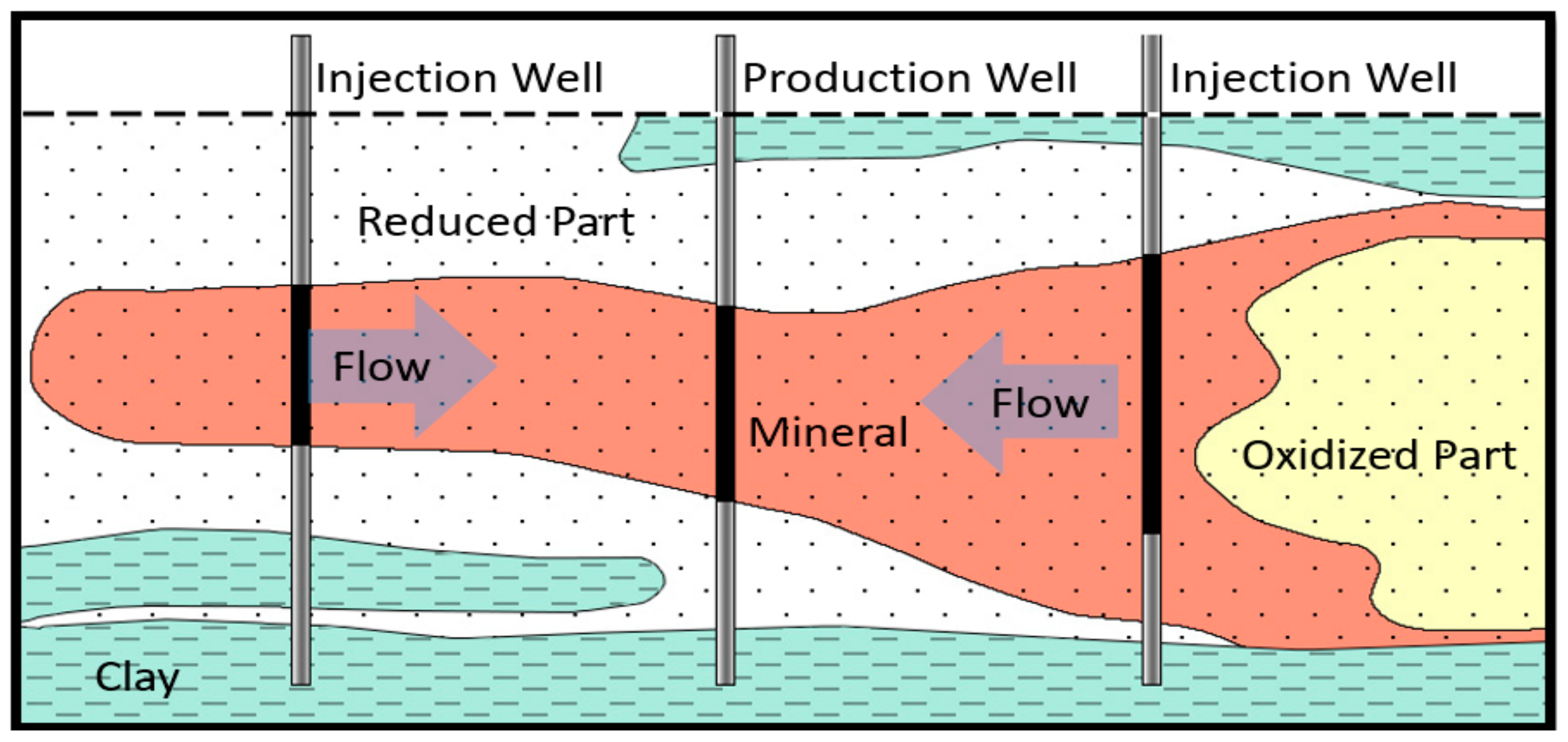
3]). The ISL method consists of injecting an acid or alkaline leaching solution directly into the ore deposit through a network of injection wells, and pumping out the productive solution containing the dissolved uranium through the extraction wells (
Figure 1). This mining method is used to develop mineral deposits with low concentration in geological formations with high permeability (
). The in situ leaching method has two advantages: high environmental friendliness and economic profitability ([
4,
5,
6]). Geological conditions and mineralization of uranium deposits in Kazakhstan make them favorable for development by in situ leaching. The leaching reagent is selected depending on the mineralogical composition of the deposit; an acid or carbonate solution can be used. In Kazakhstan, approximately 80% of uranium deposits are exploited using an acid solution made of sulfuric acid ([
4,
5,
7]). Uranium in deposits is represented as tetravalent and hexavalent complex compounds, mostly as UO
2 and UO
3 oxides, which have different dissolution rates in sulfuric acid solution. Moreover, when the solution filters through the rocks, the acid interacts with the rock mineral components, i.e., there is an additional consumption of acid that must be accounted for. However, uranium reserves are often estimated without a detailed analysis of those uranium compounds during exploration. One of the goals of this work is to improve these estimations by better accounting for the dissolution mechanism occurring during acid leaching.
Despite the fact that Kazakhstan ranks second in the world in uranium reserves ([
3,
4]), there are significant extractable problems with the remaining available reserves of uranium. To date, Kazakhstan had developed cheap uranium deposits with relative exploitation costs of less than USD 80 per kilogram. However, from 2007 to 2019, the number of such resources decreased by as much as 55% [
8,
9], and approximately 2.0 million tons of Uranium resources are left [
8]. Nowadays, it is necessary to exploit deeper mineralized layers with lower amounts of fine- to medium-grained size sandstone enriched with clay minerals (montmorillonite, smectite, and illite).
The presence of fine clay particles has two negative impacts: (i) it increases the amounts of acid by dissolving and transforming the phyllosilicate minerals (illite, muscovite, and montmorillonite) into kaolinite; (ii) it may plug productive wells. New technological breakthroughs should be developed to improve leaching technology for that depth and to better control acid consumption to decrease the production costs for extracting the remaining uranium reserves. One possible way for increasing the exploitation profitability is to model the reactive transfer processes occurring in the reservoir during the ISL extraction of uranium. Several recent works have investigated the mechanism responsible for the formation of roll-front uranium deposits [
10], analytical solutions for uranium reactive transport [
11], 1D reactive transport modeling in column [
11,
12], and 3D reactive transport modeling of uranium during in situ recovery [
13,
14]. However, the main modeling problem faced by engineers is the lack of detailed data on the mineralogical composition of the deposit, as well as the inability to monitor and analyze real processes occurring directly in the rock during mining. Moreover, the mineralogical composition of deposits can change even within the same deposit; therefore, it is easier to design elementary models with simplified chemical kinetics describing the chemical interactions of the leaching reagent with the rock. In this perspective, simplified kinetics models based on available data on the composition of deposits, and transport models are extremely relevant for industry.
Uranium deposits (or reservoir infiltration) in Kazakhstan are characterized by a rather low number of mineral components and a relatively high rock permeability (unconsolidated sand), making them favorable candidates for exploitation by the ISL method. In such deposits, uranium occurs as tetra and hexavalent compounds, mainly represented by uranium oxides UO
2, and UO
3, with different solubility rates in aqueous acid solutions. On the other hand, all uranium minerals, including complex oxides, actively dissolve in sulfuric acid solutions, while the degree of solubility may vary for the same ores in different deposits [
5]. Given the lack of data on the ratio of U
(IV) and U
(VI) in reservoirs, uranium reserves assessment can be made without a detailed analysis of uranium compounds by considering the two following chemical kinetic reactions [
5]: (i) uranium trioxide reacts with sulfuric acid to produce uranyl sulfate and water; (ii) uraninite reacts with sulfuric acid to produce uranyl sulfate and hydrogen:
The sulfuric acid solution flowing through the rock during leaching also interacts with minerals contained in rocks. In this study, no oxidizing agent has been added to the acid solution as often practiced in exploited fields for insuring the sulphate formation from uraninite. The mineralogical compositions of some deposits belonging to the Shu-Sarysu uranium province (located in a district of the Jambyl Region in south-eastern Kazakhstan) are given in
Table 1. It includes the Inkuduk and Mynkuduk horizons of the Budenovskoe deposit [
5], the Inkai deposit [
15,
16], and the Tortkuduk site of Moinkum deposits [
5].
When developing a kinetic model of uranium dissolution, it is necessary to account for the acid consumption for interaction with the minerals of the rock. It is assumed that during the leaching process, the acid bulk partially dissolves impurities without exceeding 1%; no deposit dependence has been reported [
4]. Denoted by
Minerals(s) for the rock compounds dissolved by sulfuric acid
, and by Solution
(l) for the dissolved components, the reagent reaction in the leaching solution with the rock can be written as:
where
Minerals(s) is the solid rock with a molar mass equal to the average molar mass of the sulfuric acid-soluble rock components, and a composition equal to the total sulfuric acid-soluble rock components given in
Table 1 ([
5,
15,
16]).
Based on the proposed chemical model Equations (R1)–(R3) and experimental studies of the dissolution of uranium compounds [
5], this work aims at estimating the reaction rate constants from exploitation mining data.
3. Materials and Methods for Determining the Chemical Reaction Rates from Experimental Data
History production matching of uranium deposits is limited by the lack of data on the exact in situ composition of uranium compounds in the ore and their reaction rate constants. To verify the model, and to determine the reaction rate
, uranium leaching lab experiments were conducted on materials from the Tortkuduk deposit (see
Table 1). These experimental data were reproduced and simulated numerically [
21] to estimate the reaction rate constants [
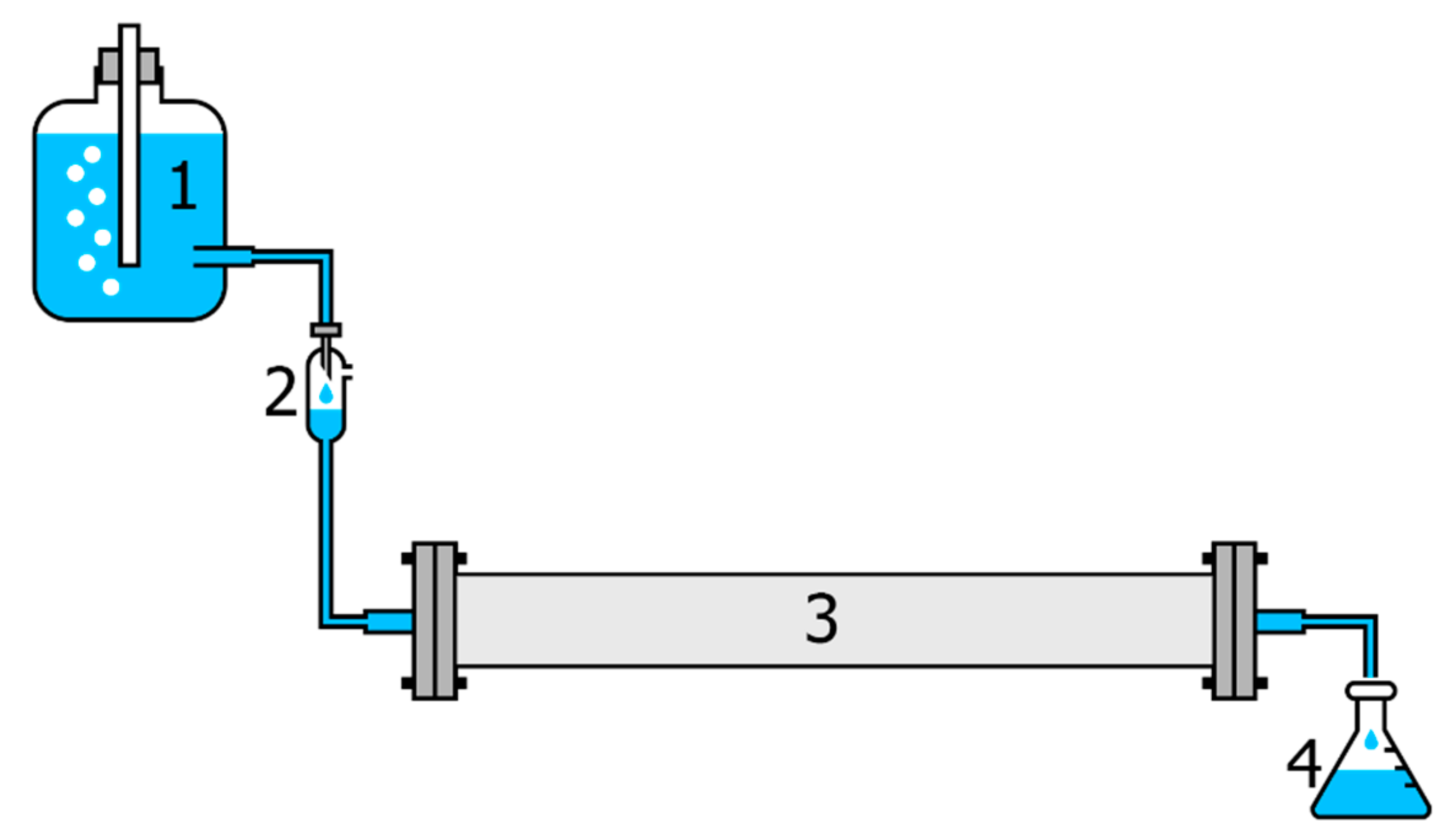
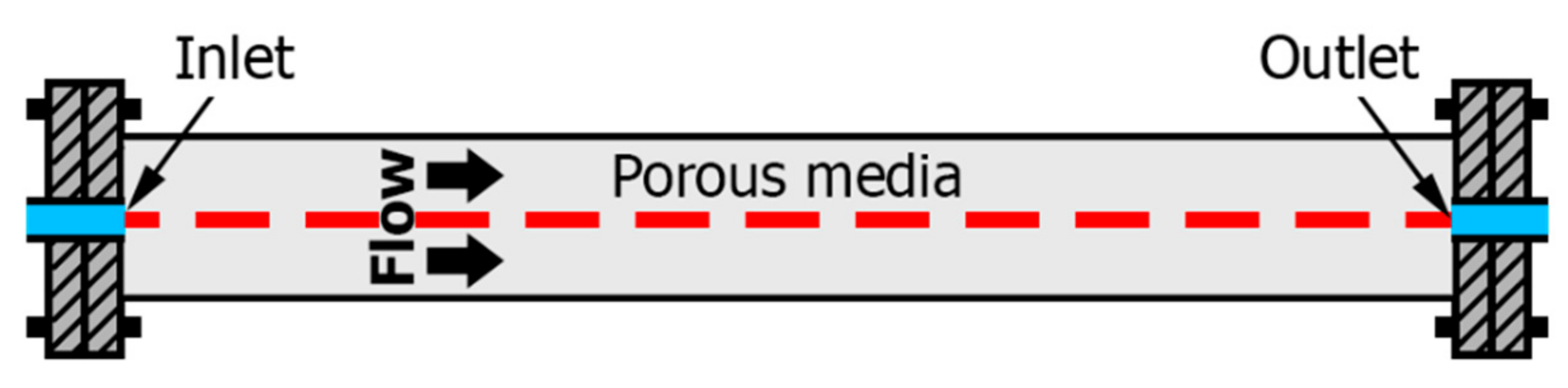
5]. The experimental device is made of a closed cylindrical tube of radius
r and length
l (
Figure 2), that receives the solution at a constant atmospheric pressure (
p = 1 atm) by a Mariotte’s vessel (
Figure 2, 1). The solution flows down the glass tube into the capillary (
Figure 2, 2) to control the flow rate in the leaching pipe (
Figure 2, 3). The ore is packed to fill the leaching pipe (
Figure 2, 3); no filter is installed at the pipe outlet. The ore material comes from the South Tortkuduk deposit. It is a medium–fine-grained sandstone without carbonates with an average uranium grade of 0.45‰ U. The geometric parameters of the experimental setup, as well as the properties of the rock, are presented in
Table 2.
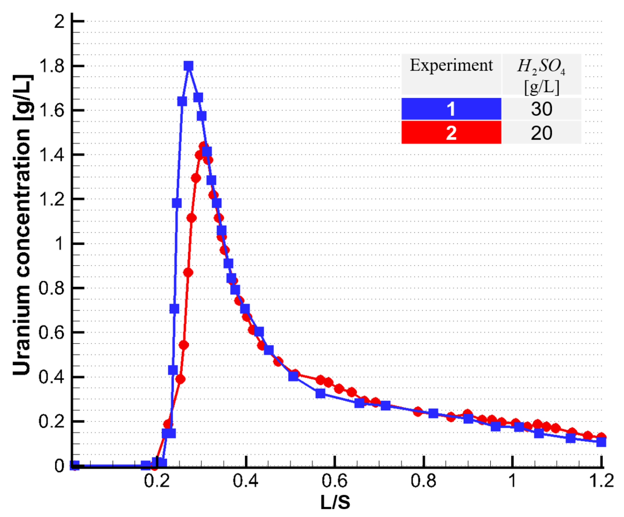
The solution passing through the pipe leaches the minerals into the receiving tank, where the concentration of dissolved minerals is measured at given regular time intervals (
Figure 2). Experimental leaching was performed in two modes with different concentrations of sulfuric acid in solution: 30 [g/L] in the first mode and 20 [g/L] in the second, which are also given as molar mass (
Table 3). This pH range mimics the field situations for which ore deposits are in situ leached with acid solutions with pH < 2 with an average of 1 [
13].
3.1. Rock Properties
In the work of Poezhaev [
5], experimental results on uranium concentration are reported as a function of the dimensionless liquid/solid (L/S) ratio, a quantity widely used in the uranium mining industry, representing the amount of leaching solution per unit of weight of the leached ore mass (L/S is typically expressed in mass units of liquid per dry mass of solid material). The typical L/S dependences on process parameters is
where
and
are the solid and liquid volumes [
], respectively;
and
the solid and liquid densities [
];
t the time [day];
Q the flow rate [
];
r and
l the tube radius and length [
], respectively; and
the solution flow rate. When the porosity
and the flow velocity
[
] are kept constant, Equation (6) shows that L/S is a linear function of the time, and thus can be also considered as a dimensionless time quantity.
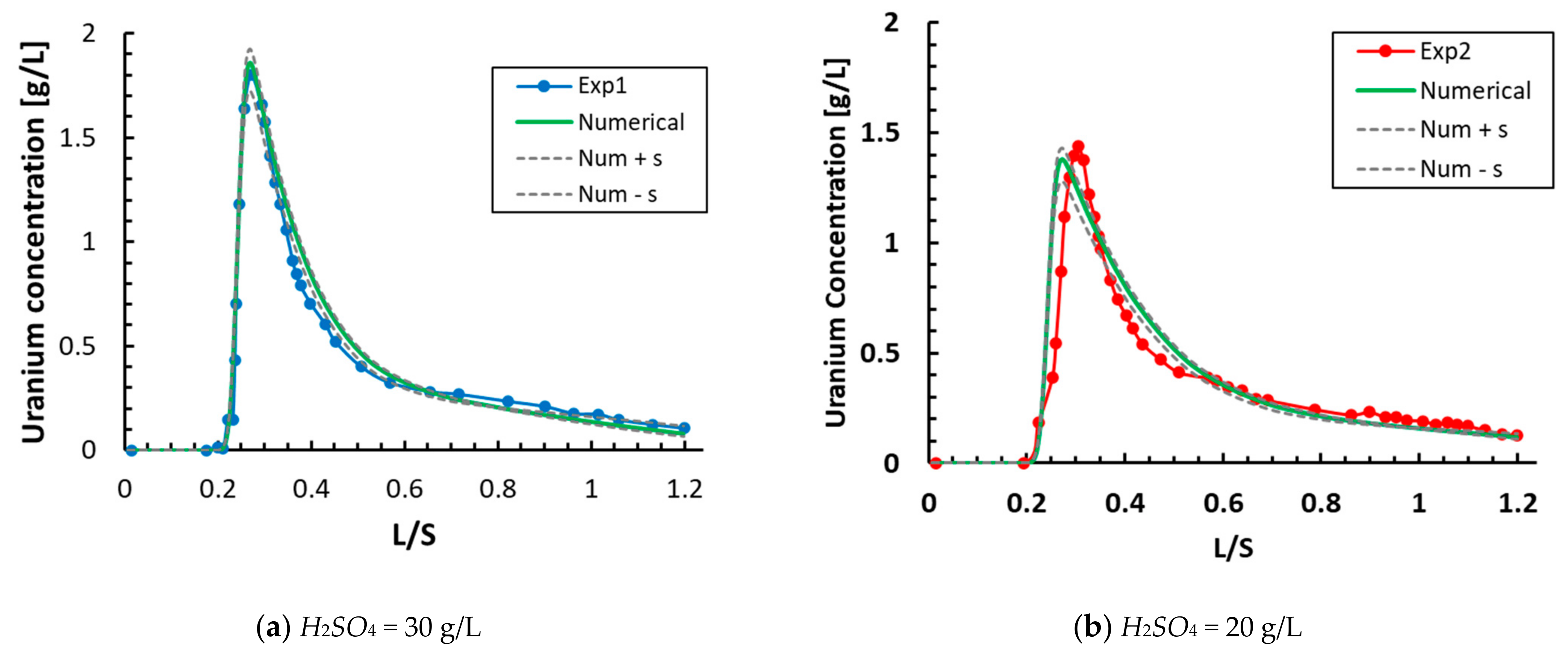
Figure 3 shows the experimental extraction curves plotted against the L/S ratio for the two modes, i.e., for the two concentrations of sulfuric acid
and 20 g/L, respectively [
5]. Dissolved mineral concentration experimental data at the tube outlet are reported in
Appendix A for both modes (see
Table A1 and
Table A2).
To estimate the reaction rates of the solution with the ore, the initial characteristics given in
Table 2 were taken into account for calculating the initial uranium stock in the tube according to:
where
is the initial uranium mass [kg] in the tube,
OreMass the initial ore mass [kg] contained in the tube,
the uranium grade [kg·kg
−1],
the solid density [kg·m
−3],
the ore volume [m
3],
the ore porosity, and
and
the tube radius and length [m], respectively. The total uranium mass
[kg] recovered during an experiment is calculated as the integral over the L/S ratio of the uranium concentration
[kg·m
−3] flowing at the tube outlet (
Figure 3):
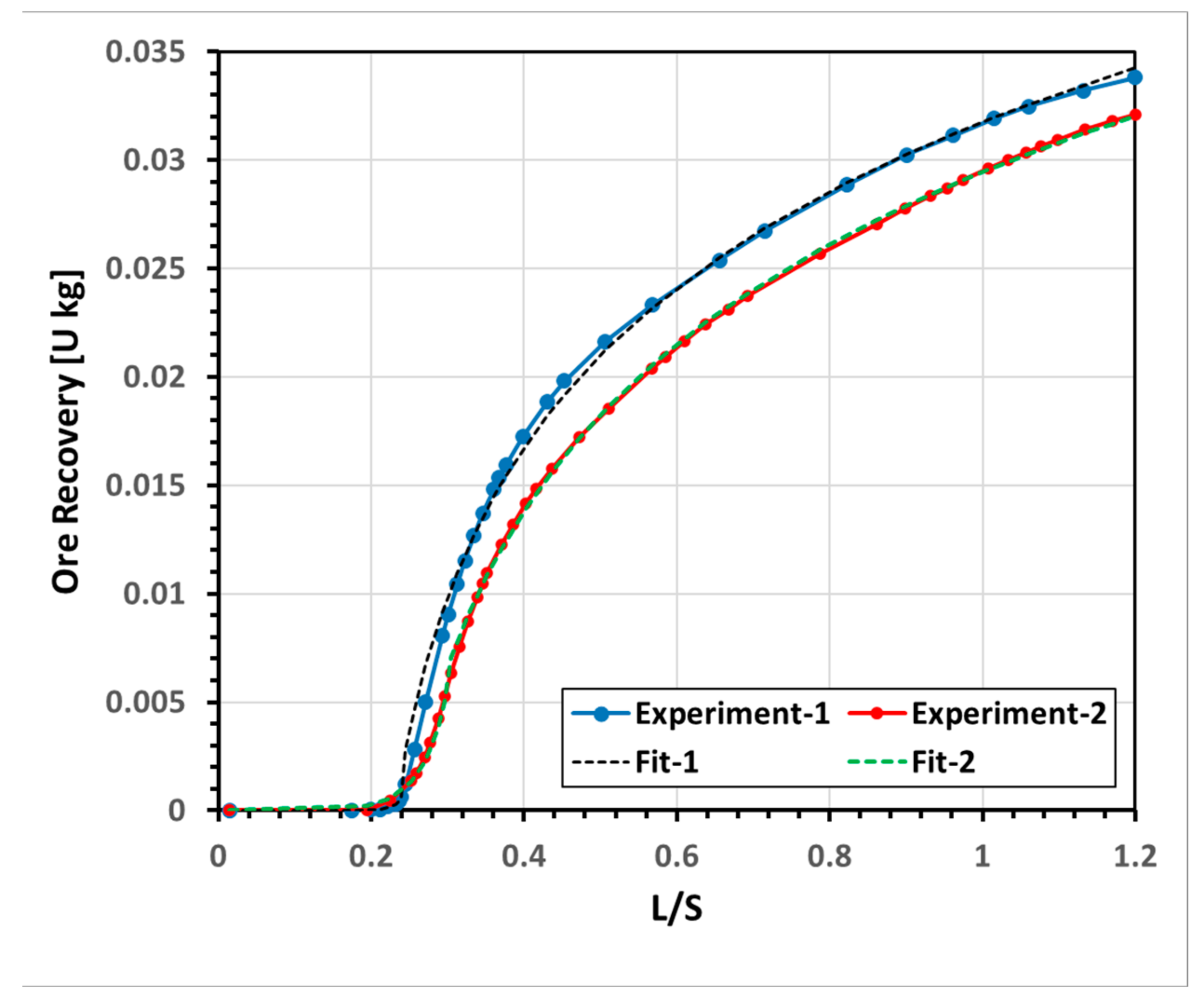
Table 4 shows the total uranium mass
[kg] extracted during the experiments together with the recovery rates for both modes, where the recovery rate is the ratio [%] of the recovered mass to the initial mass of uranium
[kg] in the tube
.
Figure 4 illustrates the dynamics of uranium extraction during experimental studies for both modes. The extraction reached 89% and 84% of the initial mass for modes 1 and 2, respectively, for an initial uranium mass of 0.038 ± 0.001 kg (
Table 4).
The above experimental data obtained by Poezhaev [
5] were used as initial parameters for simulating the leaching process to indirectly estimate the reaction rate constants for the dissolution of uranium compounds.
3.2. Numerical Experiment for Estimating the Reaction Rate Constants
For estimating the chemical reaction rates involved in the reactive transport of uranium, the above lab experiments were reproduced by numerical simulation as a simplified one-dimensional dissolution problem of a mineral in a tube (
Figure 2). The initial proportion of uranium in the ore is fixed at 0.00045 (0.45 [‰ U]), and uranium is present in the form of complex compounds as tetravalent and hexavalent uranium oxides
. However, to comply with the mass conservation law of Equations (1)–(3), the uranium concentrations in solid states are considered as a molar concentration, while the transition from one dimension to another is carried out according to:
where
is the molar concentration of uranium [mol·L
−1],
the solid density [kg·m
−3],
the uranium grade [kg·kg
−1],
the molar mass of uranium (238.03 u). The ratio between the masses of tetra and hexavalent uranium is often unknown in complex deposits; it is assumed here that uranium is in the following form
. The calculation is carried out assuming an equal proportion of both forms in the uranium deposit (
). The effect on the dissolution of uranium when varying this proportion is investigated later in the paper (see Figure 11). The leaching solution flows through the tube at a constant rate
[m·day
−1]. Schematically, the experimental setup is shown in
Figure 5.
Initial molar concentrations for uranium and minerals were taken from the described experimental data according to Equation (9):
The boundary condition (BC) for the RT model (1)–(5) in the tube are considered as follows:
3.2.1. Effect of the Dissolution Rate on the Apparent Dissolved Uranium Concentration Peak and Estimation of Reaction Rate Constants
The dissolution rate of hexavalent uranium compounds with sulfuric acid is much higher than those for tetravalent uranium [
4,
5,
6]. To estimate the dissolution rate values, a series of calculations were performed by varying
from 0.1 to 20 with a step of 0.1. This is a 3D optimal problem for finding the three unknown parameters
that best fit the uranium concentration curves
obtained in both experiments. As a result of calculations, the best agreement between the uranium concentration at the outlet and the experimental data is found to be:
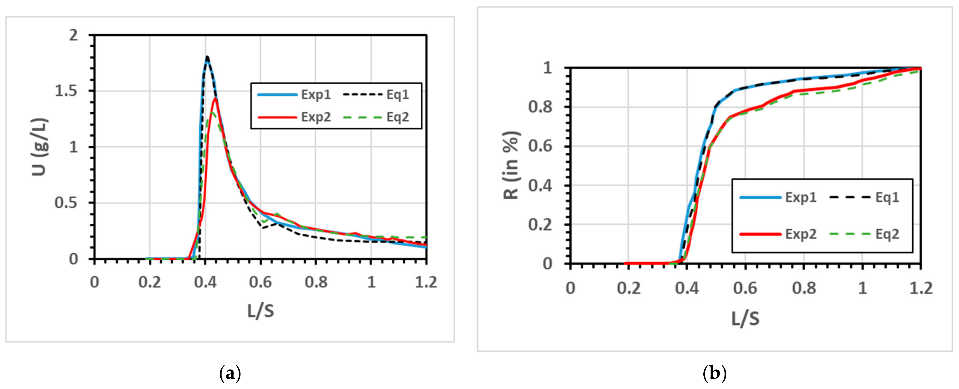
These estimated dissolution rates were used for a 1D numerical simulation of the experiments solving Equations (1)–(5). A comparison between simulated and experimental dissolved uranium concentrations at the tube outlet against the L/S ratio is presented in
Figure 6 for modes 1 and 2. The deviation of the calculated concentrations of uranium at the tube outlet was compared with the experimental data for both cases (
Table 5); the assessment was carried out according to the following parameters: normalizing the root-mean-square deviation (NRMSD), mean absolute error (MAE), and mean error (ME) [
22]. According to the obtained results, NRMSD does not exceed 7%, a rather good result given the accuracy of the initial data.
A comparison of the numerical results on the uranium concentration at the outlet with experimental data on MAE and ME shows a higher accuracy of calculation relative to the maximum value (1.80 [g/L] for the first and 1.44 [g/L] for the second mode).
The recovery calculated numerically has systematically higher values than the experimental ones in both modes (
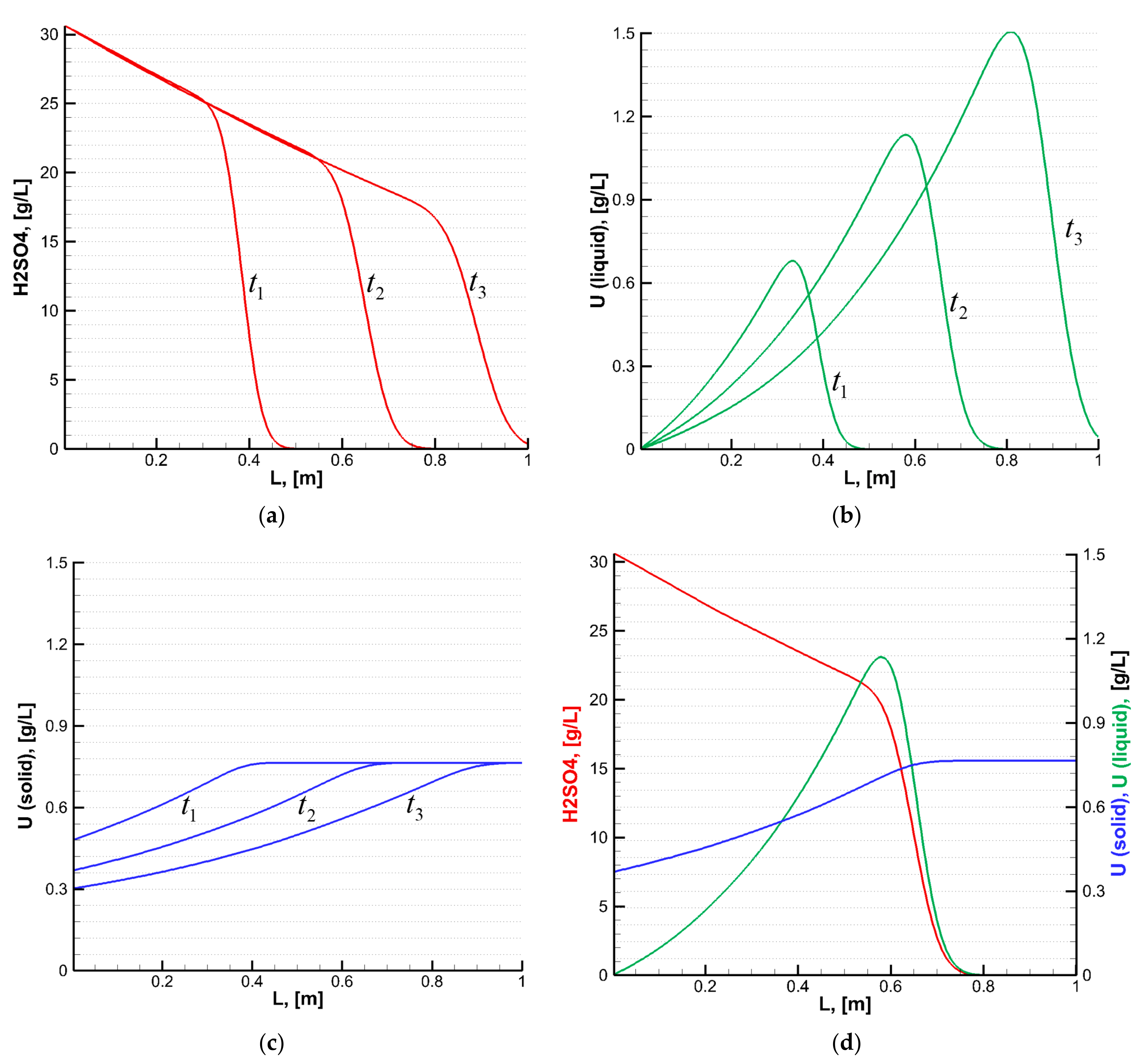
Table 6). This also depends on the accuracy of the initial data. It should be noted that, according to the laboratory experiment setup, the numerical simulation of the uranium concentration leached in the tube was performed until the L/S ratio reached the value of 1.2; some additional uranium would have flowed out if experiments were conducted for E/S ratio greater than 1.2. Using the developed model, changes in the distributions of the reagent (a), dissolved uranium concentration (b), and solid uranium concentration (c) along the tube at different times were plotted in
Figure 7. Results for the studies are plotted in
Figure 7d. They show that (i) the uranium content in solid decreases toward the tube inlet but remains quite constant along the rest of the tube where the leaching solution is already consumed; meanwhile, (ii) the leaching solution front moves toward the tube outlet while the uranium dissolution front reaches a peak at the decreasing part of the leaching solution concentration curve.
3.2.2. Effect of Filtration Rate on the Uranium Dissolution Process
The filtration rate of the solution depends on the intrinsic permeability of the ore-bearing rock, which is determined by the lithological rock structure. It also depends on pressure boundary conditions or flow rate imposed at the injection wells. Since the lithological structure is determined by nature, the only free parameter for modifying the average fluid filtration rate in the rock is the flow rate at the injection well.
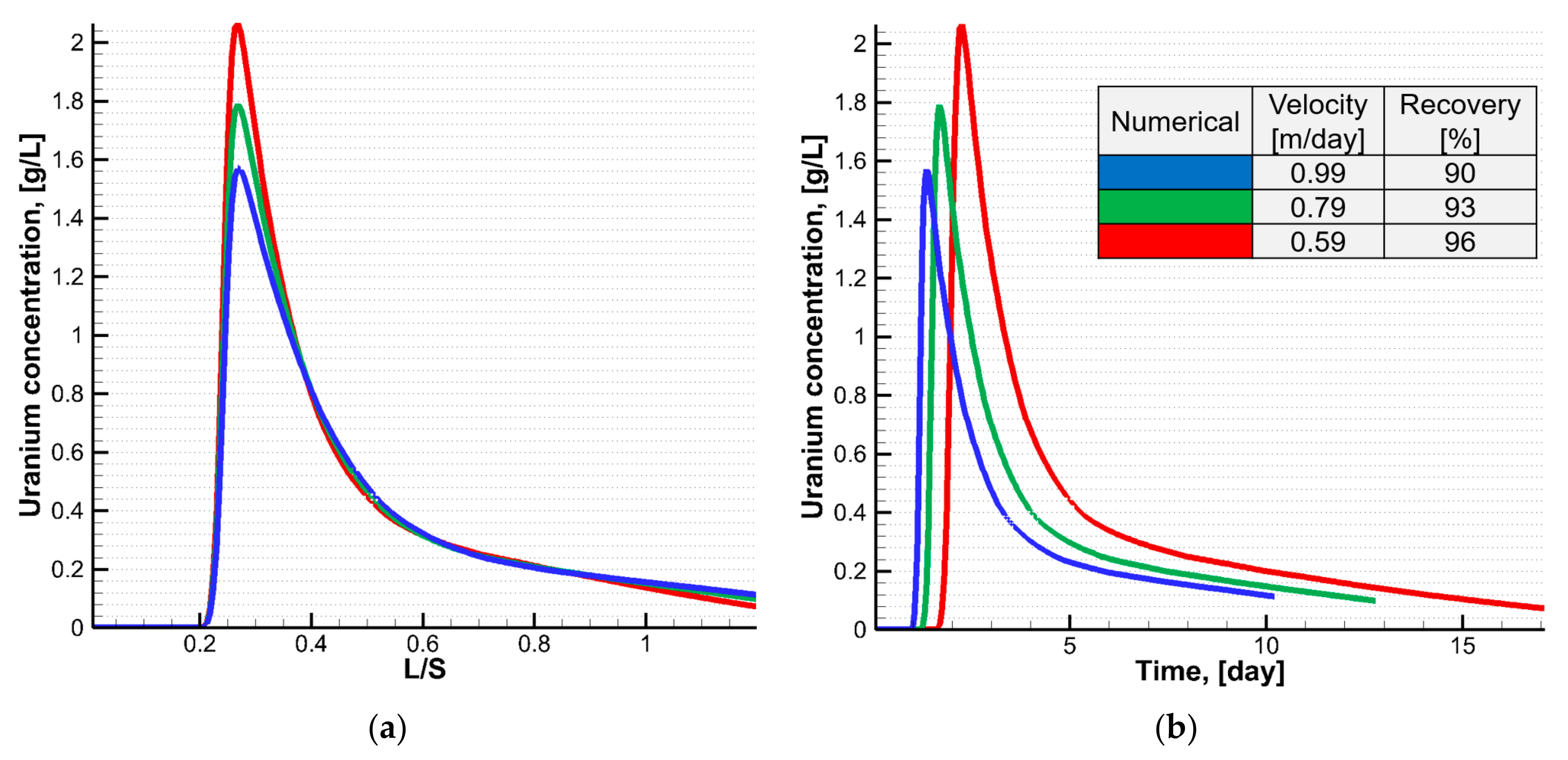
Figure 8 shows the changes in dissolved uranium concentration at the tube outlet against (a) the L/S ratio and (b) for three solution filtration rates (flow velocity), namely 0.99, 0.79 and 0.59 m.day
−1, imposed in the tube during the simulation. These numerical results show that the peak in dissolved uranium concentration at the tube outlet, the extraction recovery, and the dissolved uranium front velocity are functions of the solution filtration rate in the ore. When varying the flow velocity, the simulated maximum dissolved uranium concentration at the tube outlet is reached at the same dimensionless L/S ratio value (or dimensionless time) of approximately L/S = 0.28. The maximum uranium concentration value (peak value) at the tube outlet is quite a linear decreasing function of the solution filtration rate (flow rate) (
Figure 8a).
When concentration curves are plotted against time, it can be seen from Equation (6) that the peak is reached at a longer time when the solution filtration rate decreases (
Figure 8b). An increase in the filtration rate leads to a decrease in the uranium concentration peak magnitude at the tube outlet and accelerates the move of the dissolved uranium front for a given L/S value. The decrease in the uranium concentration peak value is explained by the uranium dissolution kinetics. At a high flow rate, the solution does not have enough time to react with the uranium-containing ore and consequently decreases the uranium extraction.
For a given L/S value, a decrease in the filtration rate leads to an increase in the peak value, the uranium extraction recovery, the processing time, and a decrease in the dissolution front speed (
Figure 8b). Thus, an increase in filtration velocity by 0.2 m.day
−1 corresponding to 25.3% of the initial value at 0.99 m.day
−1 leads to a reduction in uranium extraction by 3%, and in mining time by three (3) days, or 23.1% of the original time. Reciprocally, reducing the filtration velocity by 0.2 m.day
−1 leads to an increase in uranium extraction by 3% and an increase in mining time by four (4) days or 30.7% of the initial time. It should be noted that an increase in filtration velocity, i.e., the development terms of the deposit being faster, implies an increase in operating costs, and in general, negatively affects the price of the final product. An optimum should be found.
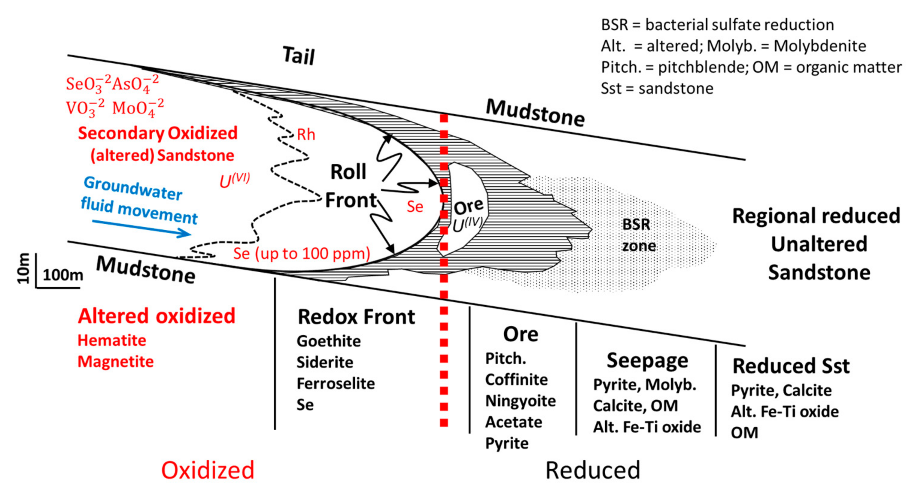
3.2.3. Impacts of the Composition of Uranium Compounds on the Leaching Process
The modeling of the mining process is complicated by the lack of information about the form in which the uranium is present in the ore, and is constrained by the average uranium grade of the rock. As mentioned earlier, uranium in the rock is presented in the form of tetravalent and hexavalent uranium complex compounds. In the proposed model, it is assumed that uranium is in the form of complex oxides of four and six-valence uranium
. In previous calculations, the ratio
was used, i.e., U
(IV) and U
(VI) were in equal proportion to the total mass. It should be noted that the U
(IV) and U
(VI) ratio may vary from one location to the other in the same deposit, in the “front” part of the roll front, U
(IV) mainly prevails since the environment is more reduced, while in the “tail” part, U
(VI) dominates with a more oxidized environment (
Figure 9), these patterns are linked to the mechanisms involved in roll front deposit genesis ([
23,
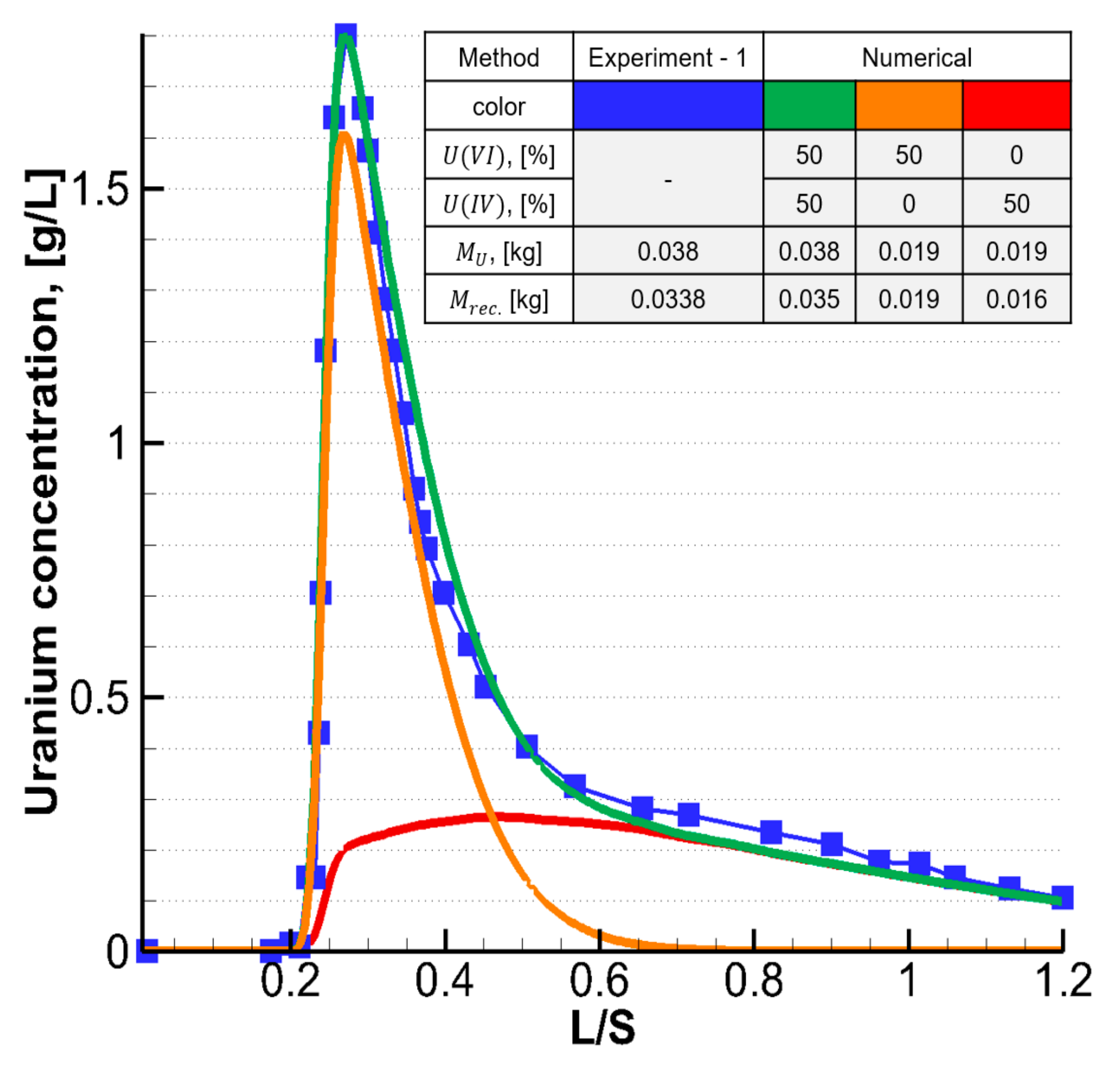
24]). In order to quantify the effect of the uranium oxidation state as observed on real deposits on the leaching process, the following three cases for the experimental mode 1 (
Figure 10) were considered:
- 1.
Rock contains U
(IV) and U
(VI) in equal proportions with a total mass
(green line) as encountered at the boundary of the roll front (
Figure 9, redox zone);
- 2.
Rock only contains U(VI), with a total mass equal to (orange line) as encountered in the oxidized zone;
- 3.
Rock only contains U(IV), with a total mass equal to (red line) as encountered in the ore/reduced zones.
Simulated results (
Figure 10) show that since the U
(IV) and U
(VI) dissolution reaction rates are not identical, a significant part of the hexavalent uranium dissolves before reaching L/S ≈ 0.8, while dissolved U
(IV) at the tube outlet is more uniform during the whole extraction period. As mentioned earlier and shown in
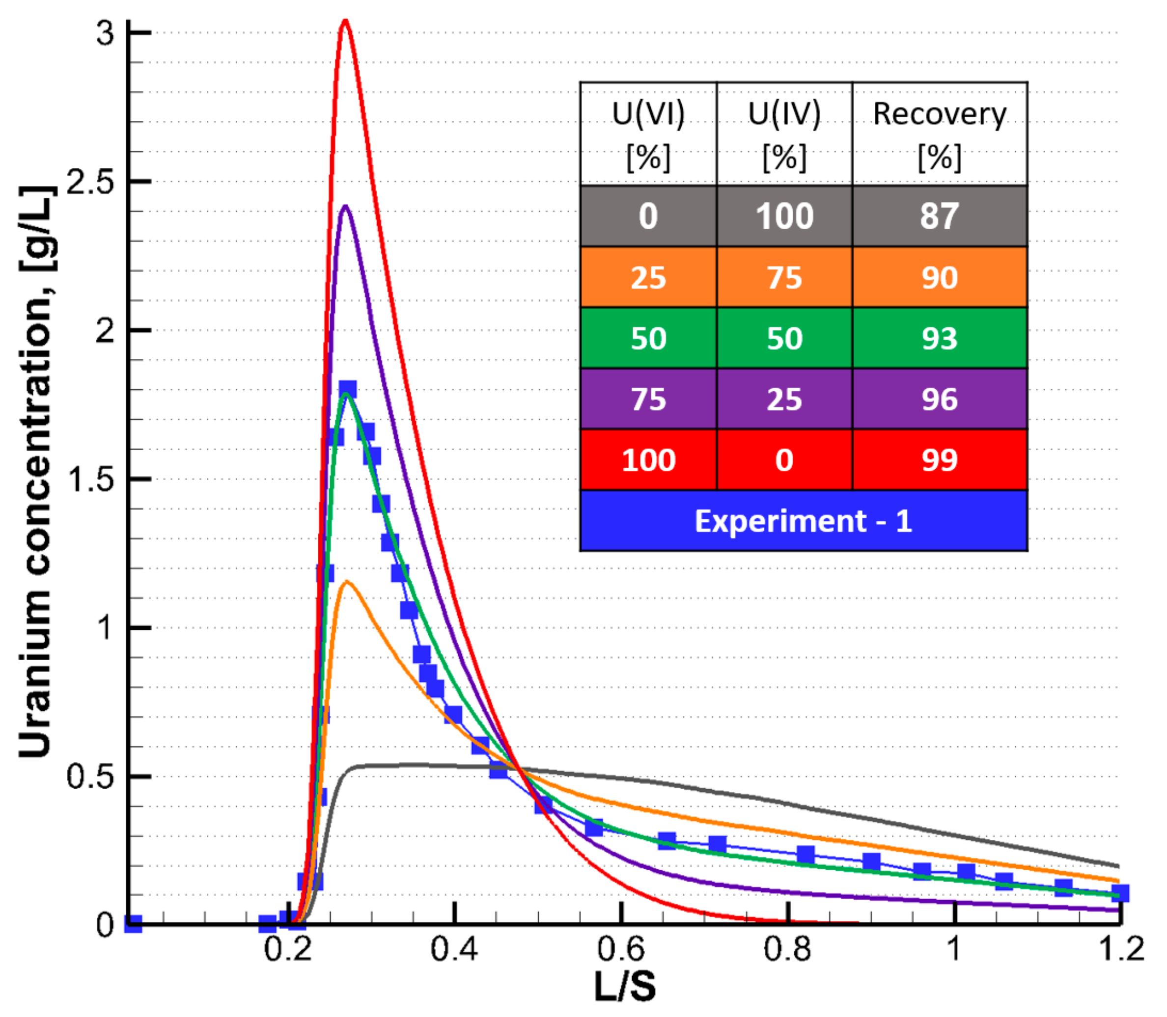
Figure 9, the uranium oxide compounds composition differs both in deposits and within a particular deposit. To analyze this influence, five different tetra/hexavalent uranium oxide ratios were investigated at constant dissolution rates (
Figure 11). With an increase in U
(IV) proportion in the rock, a significant decrease in the concentration peak value of total dissolved uranium at the tube outlet was observed, which is associated with a low U
(IV) solubility, and as a result, a decrease in recovery. Due to the high solubility of U
(VI) in sulfuric acid solutions, an increase in hexavalent uranium content in the rock increases the recovery. Through this example, it can be seen the paramount importance of accounting for the mineralogical composition, and for the U
(IV) and U
(VI) uranium oxides distribution in the deposit.
3.3. Leaching of Uranium: Analytical Kinetics Model
Experimental outlet uranium concentration (
Figure 3), and ore recovery (
Figure 4) curves are typical of leaching mechanisms corresponding to a three-time period: (i) a delay period
to
corresponding to the time necessary for the solute to cross the solid medium and to reach the tube outlet; (ii) a fast kinetics period
to
during which the acid solution leaches the uranium physisorbed at the grain surfaces and/or in micro-cracks/fractures; (iii) the last period
to
(tail of the curves) during which the kinetics involves a slower solute transfer into the grains that dissolves the remaining uranium. The last period will be studied first.
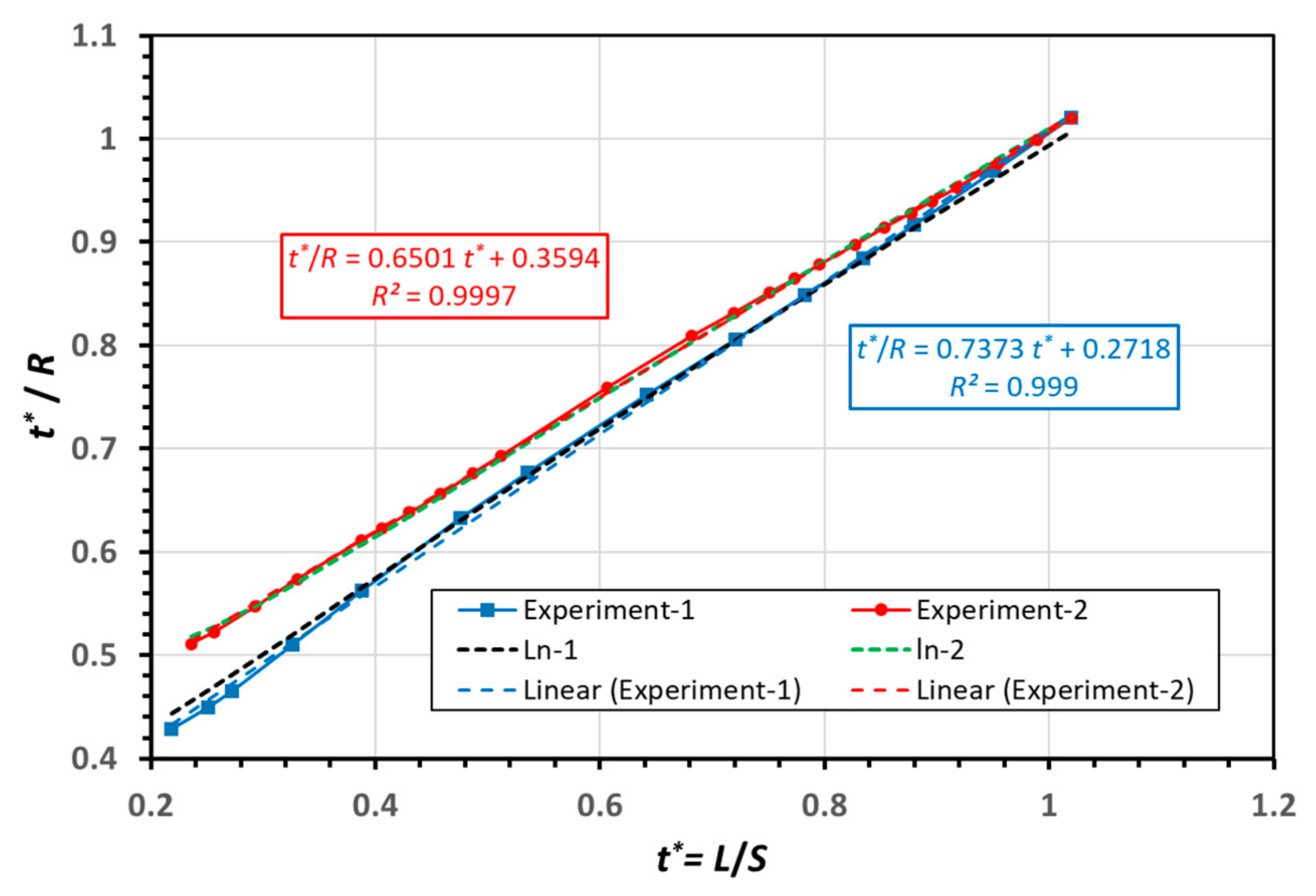
3.3.1. Adjusting the Recovery Curve Tail
Let
be the normalized ore recovery of the total uranium flowing at the tube outlet during the time
where
is the uranium total mass recovered at
, and
the total mass of uranium recovered at the end of the assay (see
Table 4),
is the dimensionless time defined by Equation (9) and counted from the delay time
(i.e.,
). The quantity
is the total uranium fraction lost by the solid at time
. The Azuara model ([
25,
26]) states that the total leachable fraction
at time
is proportional to the remaining part of uranium in the solid phase according to
with
the reaction advance rate, a linear function of time
whose slope
is a constant at fixed temperature and pressure, dependent on the component to be extracted, and
the fraction of solute loss at final equilibrium condition
. It leads to the following linear model:
The two parameters
and
are estimated by fitting the experimental data of
vs. time
to the linear model Equation (11).
Figure 12 shows that the two experimental data perfectly fit the Azuara linear model given by Equation (11). Least squares estimates of the two parameters together with the starting time
are given in
Table 7. The Azuara linear model is compared to the log model:
The two parameters
and
were fitted by minimizing the mean absolute errors with experimental data; they are given in
Table 8. The resulting fitted logarithm curves are plotted on
Figure 12 and shows that the experimental data reproduced the same relationship as described by the Azuara model or by the exponential model. On a practical point of view, both models can be considered as similar.
3.3.2. Adjusting the Fast Leaching Phase
The fast normalized ore recovery phase is characteristic of an exponential model in which the increase
in the total leached uranium amount
during an infinitesimal time interval
is proportional to the already leached amount of
at time
(1st-order kinetics) according to ([
25,
26,
27,
28]):
The two parameters
and
are estimated by fitting the experimental data of
vs. time
to a linear model. Least squares estimates of the two parameters together with the starting time
are given in
Table 9. The ore recovery curves resulting from the merging of the Azuara and exponential models adjusted onto the experimental data are plotted in
Figure 4 showing a perfect fit. Introducing the indicator function
(equal to 1 if
and 0 elsewhere), the final model can be written as:
The normalized ore recovery
must be multiplied by the total mass ore recovery
(
Table 9 or
Table 4) for obtaining the uranium mass recovered
[kg] at time
t reported in
Figure 4.
3.3.3. Adjusting the Concentration Curves
The uranium concentration curves can be derived from Equation (8) by derivation of the above model Equation (14), or by a direct fit of the experimental data. A simplified best fit for the two experimental data (reported in
Figure 6a,b) is given by a bi-compartmental exponential model with a tail at a constant value for a large time
. The model writes:
The four parameters
and
estimated by minimizing the mean absolute errors with experimental data are given in
Table 10; the resulting analytical curves compared to experimental data show a perfect fit (
Figure 13). The bi-compartmental exponential model fits the increase/decreasing part of the concentration curve and fits more or less the peak concentration (better for the 1st experiment than for the 2nd one), but decreases too rapidly for a time greater than
necessitating the addition of a constant term
(uranium contained in residual grains is continuously leached by a slower kinetics). Ore recovery data curves are relatively well adjusted with a relative mean absolute error (RMAE) of approximately 5.5% (Exp.1) and 8.7% (Exp.2), respectively. The above analytical models can be used to indirectly estimate the reaction rate values
,
and
using Equations (1)–(5).
4. Modeling of Uranium Leaching on a Full-Scale Deposit Site
The proposed kinetics model and previously estimated reaction rate values were applied to a full-scale field case study experiment, namely the Budenovskoe deposit, to reconstitute the history matching production [
29,
30]. Required data for modeling the exploitation of the Budenovskoe deposit were taken from the open literature [
29,
30]; the deposit area totals 23,700 m
2 with average productivity of approximately 15.25 [kg m
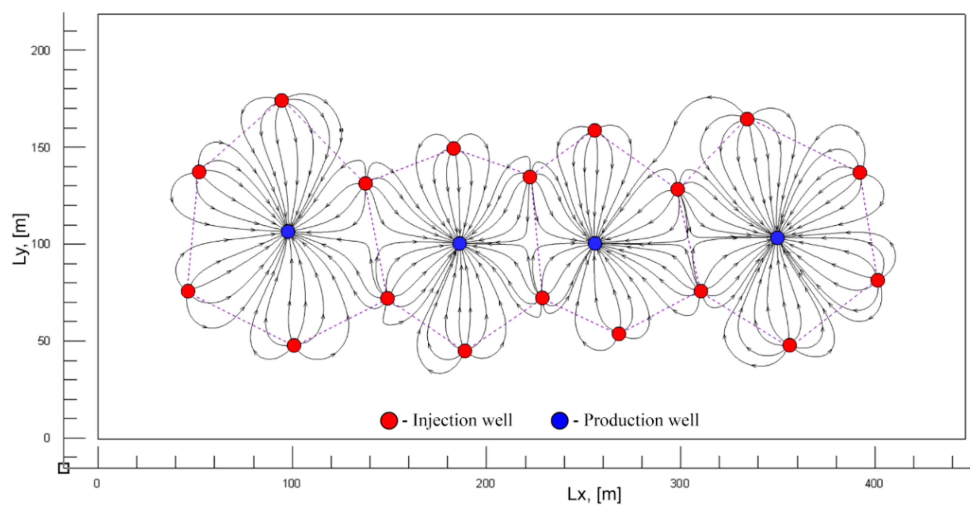
−2]. The deposit was exploited by a grid network of 4 hexagonal cells involving 18 injection and 4 production wells. The main characteristics of the site are reported in
Table 11. The hexagonal well pattern is shown in
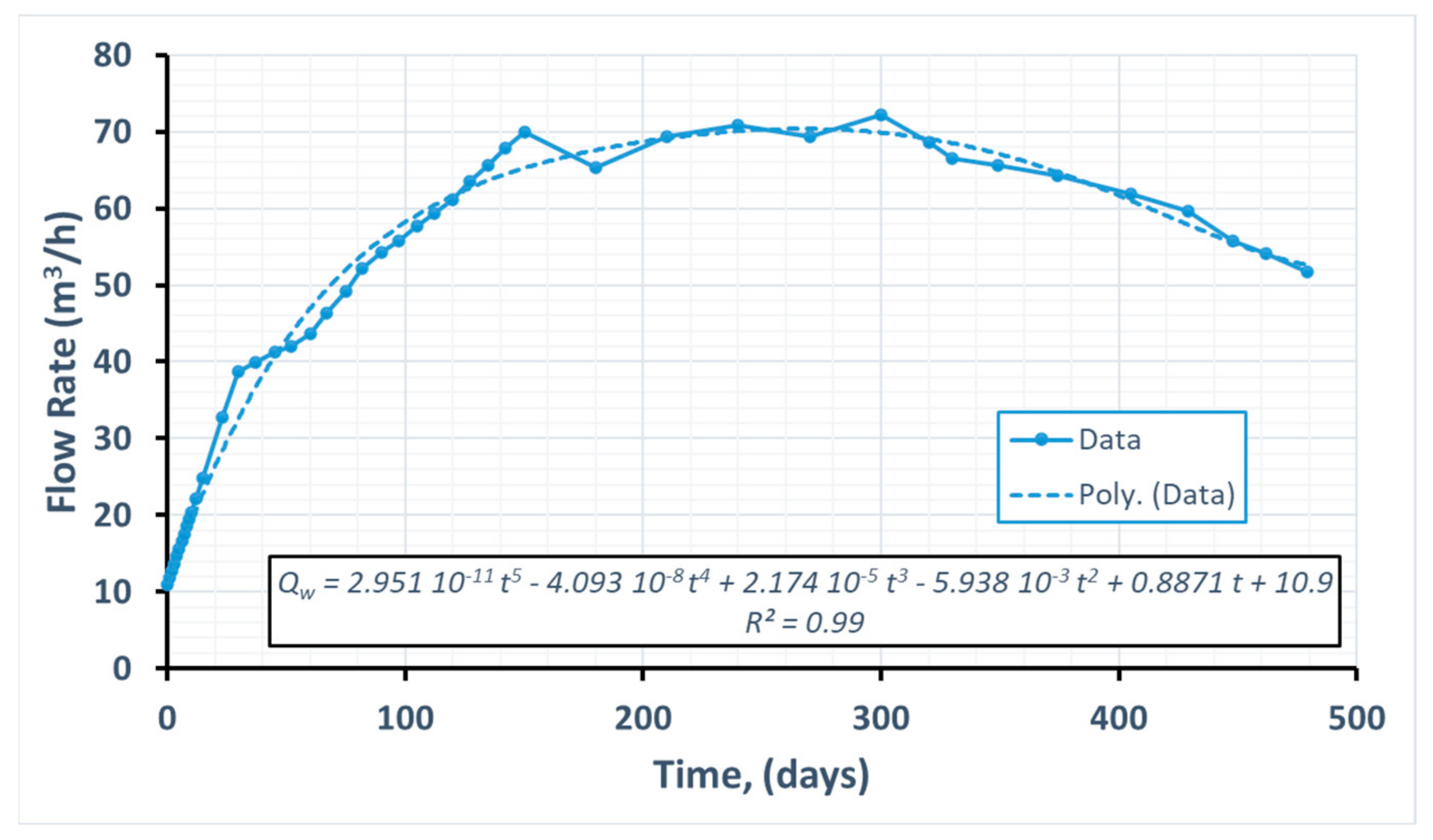
Figure 14, with injection wells in red, and production wells in blue. The leaching operation lasted 16 months. According to the published exploitation procedure, the total production wells flow rate varied over time according to
Figure 15. Acidification of blocks was carried out in an active mode for 65 days, and the solution to injection wells was simultaneously supplied by pumping the reservoir formation water to keep the flow balance.
During the first ten (10) days, the acidity of the leaching solution gradually increased from 5 to 20 g/L, then stabilized at a 17–19 g/L level. Upon reaching a pH value of 3.0–3.5, the acid concentration in the solution gradually decreased to 15–12 g/L, followed by a decrease to 10–9 g/L at pH = 2.5. Using the Mass Conservative Law and the Darcy Law [
22,
30], the pressure field, the velocity field, and the streamlines in the reservoir were calculated under the action of the well network and on the imposed constant flow injection boundary conditions (
Figure 14).
Figure 15 illustrates changes in the total flow rate/productivity
[m
3·h
−1] of wells over the time. The uranium dissolution process with a sulfuric acid solution was simulated according to the model given by Equations (1)–(5), using the flow rate values calculated in the reservoir. The calculations used the chemical model describing the interaction of the solution with the ore Equations (R1)–(R3), as well as the dissolution rate coefficients determined from the experimental study. Due to a lack of data on the solution distribution in the reservoir, a detailed comparison between numerical and experimental results is not possible. The work by Patrin [
29] presents only the integrated characteristics of the changes in the uranium content in the productive solution and recovery.
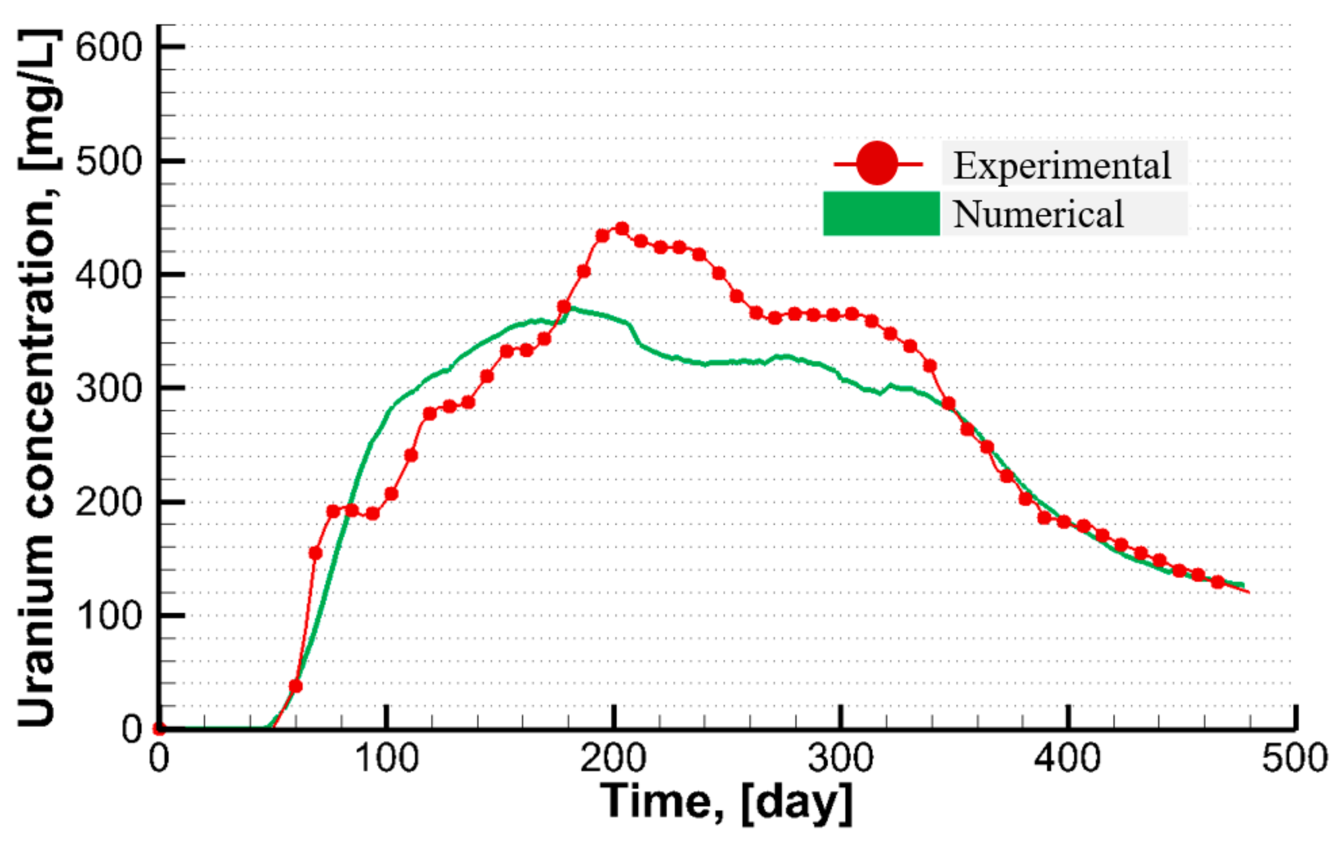
Figure 16 shows changes in uranium content over time in uranium in the solution at the production wells (producers) with experimental data in red and numerical calculations in green. Due to the lack of detailed data on the distribution of uranium compounds in the ore, an equal proportion (i.e.,
n = m = 1) of uranium was used in the calculations.
This assumption of a constant proportion of U
(IV) and U
(VI) could explain the poor fit observed on
Figure 16 between the simulated and the observed uranium content in the solution measured at the production wells. A comparison of deviations in the dynamics changes in uranium concentration at the extraction wells (producers) with experimental data shows that the normalized root-mean-square deviation (NRMSD) does not exceed 0.17% of the maximum value, while the mean absolute (MAE) and mean (ME) errors are 30.85 and 15.21 mg L
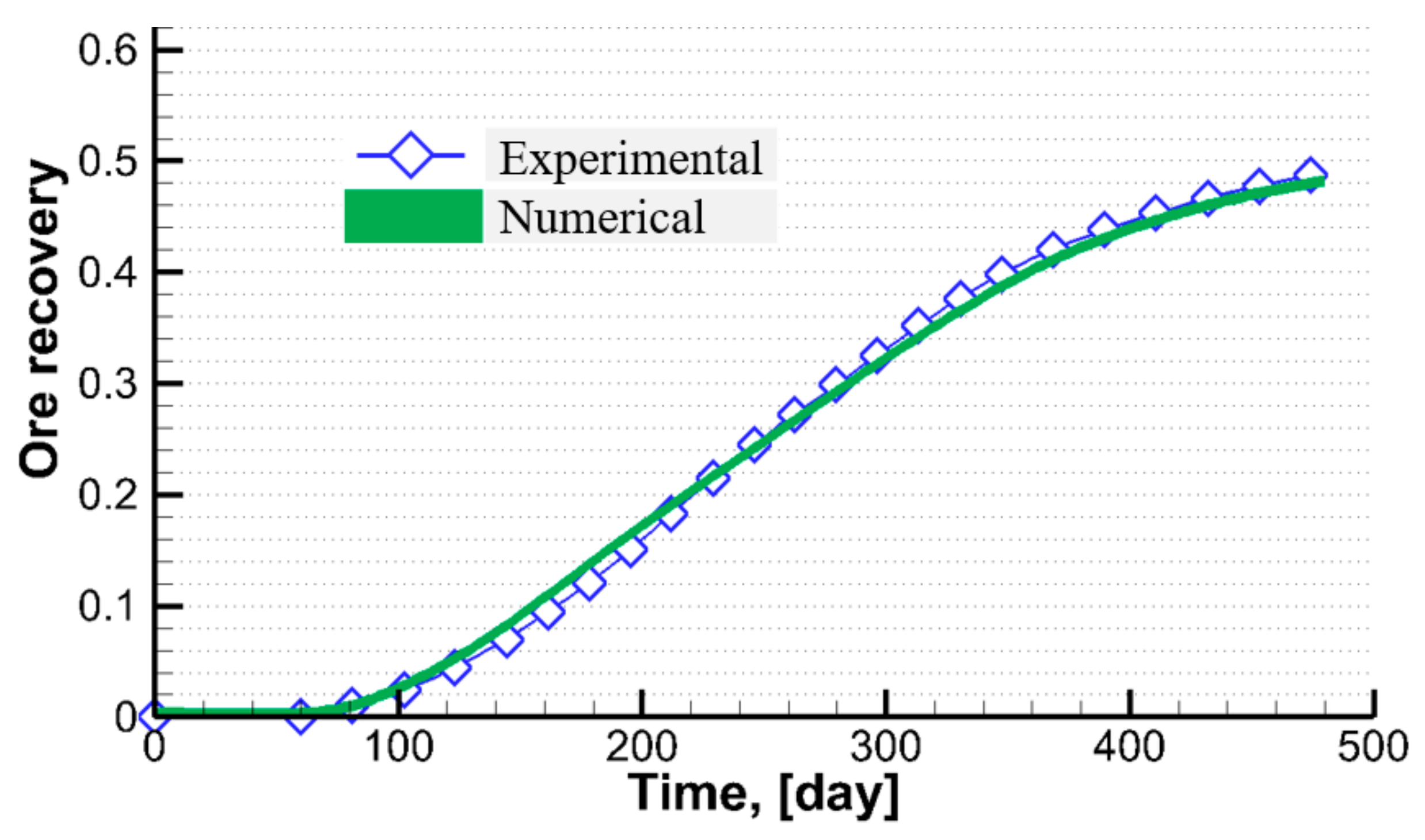
−1, respectively. The change in leached uranium recovery over time in the reservoir was determined, and numerical calculation compared to experimental recovery curve provided by the exploitation, shows good agreement (
Figure 17). This fit is better than for uranium concentration because recovery is a cumulative quantity.
Table 12 shows a comparison of the deviations calculated between the experimental uranium extraction data and the calculated data; it shows a fairly high level of agreement.


 ,
, 


