Abstract
The identification of minerals is indispensable in geological analysis. Traditional mineral identification methods are highly dependent on professional knowledge and specialized equipment which often consume a lot of labor. To solve this problem, some researchers use machine learning algorithms to quickly identify a single mineral in images. However, in the natural environment, minerals often exist in an associated form, which makes the identification impossible with traditional machine learning algorithms. For the identification of associated minerals, this paper proposes a deep learning model based on the transformer and multi-label image classification. The model uses transformer architecture to model mineral images and outputs the probability of the existence of various minerals in an image. The experiments on 36 common minerals show that the model can achieve a mean average precision of 85.26%. The visualization of the class activation mapping indicates that our model can roughly locate the identified minerals.
1. Introduction
The identification and classification of minerals are indispensable in geological research [1,2]. Experts identify the minerals by observing the color, transparency, luster, and other physical characteristics of the hand specimen, or the optical properties of the minerals in the thin-sections under the microscope. Advanced instruments such as X-ray diffraction, electron probe, Raman spectroscopy, scanning electron microscope, and energy dispersive X-ray spectroscopy can improve the identification accuracy [1,2], but it is time consuming and costly. Compared with the above instruments, cameras are easier to operate, more efficient and convenient, and much cheaper. Therefore, artificial intelligence identification of minerals in photo images has been one new important trend [1,2].
Deep learning, which is now the most used method in the field of artificial intelligence, is widely applied in the field of photo images identification and has the highest performance [3]. Therefore, many research used deep learning methods in mineral photos identification and achieved good results [4,5,6,7,8,9,10]. Although deep learning methods are effective in mineral identification, they can only identify a single mineral that occupies the largest proportion in the images. On the other hand, in the natural environment, several different minerals in rocks or ores are more common, which results in the presence of multiple minerals in an image. So new methods need to be brought out to identify the multiple minerals in an image.
Multi-label classification [11,12,13,14] has been used in applications like protein subcellular localization [15,16], automatic diagnosis of Alzheimer’s disease [17], remote sensing image processing [18], and so on. These research all have one thing in common: each image contains multiple objects to be recognized and these objects are related in some way. Associated minerals contain multiple minerals to be identified, so multi-label image classification can be used in mineral identification.
In this paper, a deep learning model based on multi-label image classification is designed to identify minerals. As shown in Section 3, the model first extracts mineral features from the image and then correlates each mineral labels embedding with mineral features by using a transformer decoder. The probabilities of the existence of minerals in the image will be output to the user. Software according to the method was implemented and achieved the mean average precision of 85.26% when multiple minerals exist in an image for 36 common minerals. Compared with other work, our method can identify multiple minerals in an image with high precision. Therefore, our work can provide more information to the users. Generally, our method identifies the minerals in a quicker, easier and more economical way compared with the traditional mineral identification methods, which will benefit the related geological work.
2. Dataset
Because a large number of known images are required to teach the artificial intelligence models to identify the minerals [1,2], we use the same photo images of Zeng et al. [4] to teach and test our model. The photo images are from Mindat.org [19]. However, unlike Zeng et al. [4] used only a single label for an image, no matter how many minerals the image contains, we use multi-labels for the image, as shown in Figure 1. Label (s) here means the true mineral (s) exist in an image. As can be seen from Figure 1, the mineral images contain a variety of minerals, and it is difficult to distinguish, especially for the third one. For the third image, most people may think it contains three minerals, but actually only two minerals exist.
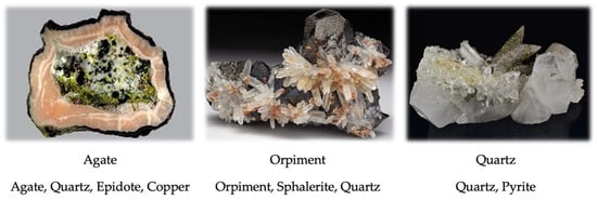
Figure 1.
Three example images in our dataset. The first row is the single label used by Zeng et al. [4], and the second row is the multi-labels used in the paper.
There are 183,688 images of 36 mineral categories with 232,467 labels in our dataset and all images are resized to 384 × 384. The number of minerals contained in an image and the number of this kind of images are shown in Table 1. In the 183,688 images, 142,508 images contain only one mineral, 34,619 images contain two minerals, and 6561 images contain more than two minerals. The minerals and their number of labels in our dataset are shown in Table 2. The 183,688 images are divided into training set, validation set, and test set at the ration of 18:1:1. The training set is used to teach the model, the validation set is used to determine when the training can stop, and the test set is used for evaluating the performance of the model.

Table 1.
Number of minerals in an image and the number of this kind of images.
Table 2.
Mineral names and the number of labels for each mineral.
3. Method
A multi-label image classification model is proposed in the paper to identify the multiple minerals in a photo image. The model first extracts mineral features from the image and then correlates the features with the known mineral (s) by using a transformer decoder. The probabilities of the existence of the 36 minerals in the image is output to the user. The probability here means how likely a mineral exists in an image. The architecture of the model is shown in Figure 2, which consists of two parts: mineral feature extraction (Part 1) and label probability query (Part 2).
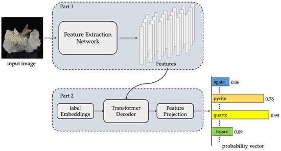
Figure 2.
The mineral identification model based on the multi-label image classification. After a mineral image is input into the model, the probability of the presence of each mineral is output.
For an input mineral image ) is the height and width of an input mineral image, 3 is the RGB channel of the image), its height and width is resized to first. Then, the resized image is fed to Part 1 for feature extraction, and the feature map of the mineral image is obtained. Here, the Feature Extraction Network can be any convolutional neural network or any transformer-based network. If the Feature Extraction Network is a convolutional neural network, the height and width of the feature map are flattened to one dimension to meet the input requirements of the transformer decoder in Part 2.
After extracting the mineral features, the transformer decoder in Part 2 models the features and the label embeddings to acquire the probability of the existence of each mineral in the image through its attention mechanism. Finally, the model obtains the probability between 0 and 1 for each mineral via the Feature Projection operation. As before, the probability here means how likely a mineral exists in an image.
3.1. Feature Extraction Network
Many feature extraction networks have been proposed with the rapid development of computer vision in the past few years, such as ResNet [20], MobileNet-V2 [21], Big Transfer [22], Vision Transformer [23] and so on. Among them, Vision Transformer (ViT-B/16) applies a standard transformer encoder [24] for image classification by splitting each image into a sequence of embedded image patches. ViT is suitable for transfer learning [23] and has become one of the most widely used transformer-based feature extraction network, so ViT-B/16 is used in the paper as the feature extraction network. The structure of the ViT-B/16 we used is shown in Figure 3. The input mineral image is resized to and is divided into multiple patches. In Linear Projection of Flattened Patches layer, a convolution kernel () is operated on those patches and a feature map of () is got, then it is flattened and a feature matrix of is obtained. In Position Embedding layer, position information is added, and the matrix turns to and is fed to the Transformer Encoder. After the Transformer Encoder, the position embedding is removed, and the matrix is reshaped to and a convolution operation is made to project the features from the shape of to the shape of to meet the dimension requirement in Part 2 (2048 is the dimension of the transformer decoder in Part 2).
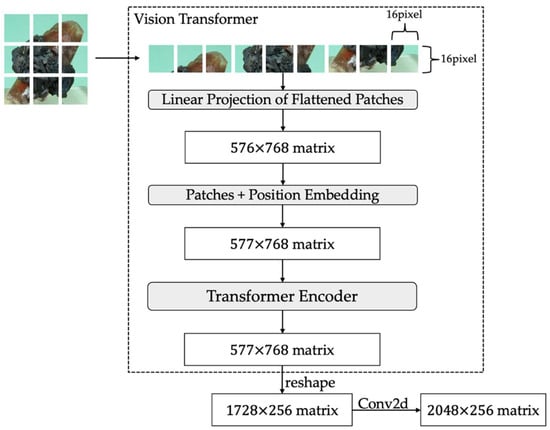
Figure 3.
The structure of the ViT used in the paper.
3.2. Transformer Decoder
For an input mineral image, after the feature extraction in Part 1, its feature matrix of is obtained. Additionally, then the feature matrix is reshaped to and fed to Transformer Decoder to query the label probability of each mineral.
The architecture of the transformer decoder of the paper is shown in Figure 4, which has 3 layers as that in paper [24]. The 3 layers are a multi-head self-attention, a multi-head cross-attention and a fully connected feed-forward network (FFN), followed by a layer normalization [25] and a residual operation [20], respectively. The label embedding is a matrix of (36 is the number of types of minerals need to be identified) and is learned as that in DERT [26].
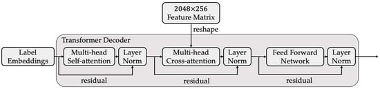
Figure 4.
The transformer decoder of the paper.
Multi-head attention that consists of three matrices, query (Q), key (K) and value (V) is used to collect the information from different representations at different locations simultaneously, which is impossible for using only a single attention head. The correlation between the minerals is got by multiplying Q and K and the attention is obtained, as shown in Equation (1). In Equation (1), is the dimension of K.
For the multi-head self-attention block, Q, K and V all come from the label embedding (). For the multi-head cross-attention block, Q is from the self-attention block’s output, K and are from the feature matrix in Part 1.
After going through the Transformer Decoder blocks, the output matrix is obtained. In the Feature projection layer, the output matrix of the Transformer Decoder is flattened and fed to a linear layer to get the vector of dimension 36. After that, the vector of 36 is operated by a sigmoid function, the model gets the probability between 0 and 1 for each mineral.
3.3. Asymmetric Loss Function
As before, an input mineral image is denoted as , and there are K categories of minerals in total. The true label of is denoted as = [, …, ], where {0, 1}, k = 1, …, K, = 1 if the k-th mineral is present in image , otherwise = 0. The classification result of is denoted as = [, …, ], where [0, 1], k = 1, …, K.
The loss function can quantify the distance between the true label and the classification result . In our research, due to the problem of imbalanced distribution of mineral images which is inherent in multi-label classification [12], Asymmetric Loss (ASL) [27] function is used. ASL uses modulating factor [28] to reduce the weight of the loss function of high-confidence images and uses focusing parameters [27] to smooth the loss function so that the model can focus more on harder images during the training. The Asymmetric loss function used in this paper for each training mineral image is shown in Equation (2).
In Equation (2), and are two focusing parameters, and by setting , the contributions of harder samples during training can be better controlled [27]. In our research, we set and as stated in [27], then the loss function is like that in Equation (3).
4. Experiments
The proposed model was implemented under the Linux CentOS platform and a 12 G Tesla p100 s were used. We adopted the official PyTorch implementation for both the Feature Extraction Network and the Transformer Decoder. The model was trained for 50 epochs with batch size 16 using an AdamW [29] optimizer with a learning rate of 1 × 10⁻⁵. RandAugment [30] was used to improve the performance of our model on the unseen mineral images. To evaluate the performance of our model, 9184 images in our dataset unseen for the model were tested.
4.1. Evaluation Metric
In multi-label classification, the mean average precision (mAP) [12,13] is usually adopted to evaluate the performance of the models. The calculation of mAP requires the average precision (AP) of each mineral category. Additionally, the calculation of AP requires precision and recall.
In artificial intelligence, positive and negative samples are defined according to the ranking of the probability of the classification result. For top-n, the first n in the ranking are positive samples, and the rest are negative samples. In the positive samples, those that are the same as the truth are called true positive (TP), and those that are not the same as the truth are called false positive (FP). Additionally, in the negative samples, those that are the same as the truth are called true negative (TN), and those that are not the same as the truth are called false negative (FN). Obviously, TP + FP + FN + TN = TNS (Total Number of Samples). Precision and recall equations are defined, as shown in Equations (4) and (5).
After calculating the precision and recall corresponding to top-1 to top-n according to Equations (4) and (5), AP of a mineral category can be calculated according to Equation (6), where N = TNS. In Equation (6), and are the precision and recall under top-n.
AP evaluates how good the model is in one mineral category, mAP evaluates how good the model is in all minerals categories.
4.2. Experimental Results
4.2.1. Feature Extraction Network Selection
As stated in Section 3, our Feature Extraction Network can be any convolutional neural network or any transformer-based network. In order to explore which network is more suitable for identifying multiple minerals in an image, four widely used networks, MobileNet-V2 [21], Big Transfer [22], ResNet [20], ViT [23] were tested as the feature extraction networks. The experimental results are listed in Table 3. In addition to mAP, the number of parameters in million and the training memory cost in megabits are also given. From Table 3 we can see, ViT-B/16 has the highest mAP (85.26%) and greatly exceeds the MobileNet-V2 and ResNet-101 and is also higher than the recently proposed state-of-the-art transfer learning model Big Transfer. Although ViT-B/16 has twice the number of parameters as ResNet-101, the training memory cost of ViT-B/16 is not much higher than ResNet-101. Actually, we have also tried the Swin Transformer [31] as our feature extraction network, but unfortunately it cannot work on our platform due to the memory limitation. It can be inferred that our model can achieve better performance if better computers or more advanced CNN or transformer-based networks are used.
Table 3.
Experimental results of the four feature extraction networks.
4.2.2. Loss Function Selection
In addition to the ASL used in the paper, other loss functions available for multi-label classification were also tested with ViT-B/16. The results are shown in Table 4. From Table 4 we can see that ASL used in this paper achieves higher mAP than Binary Cross-Entropy and Focal Loss [28]. This shows that the ASL can better handle the label imbalance problem.
Table 4.
Mineral identification results using different loss functions based on the model of the paper.
4.2.3. Experimental Results with ViT and ASL
The average precision (AP) of each mineral category of our model using ViT-B/16 as feature extraction network and ASL as the loss function is shown in Figure 5. Figure 5 shows that AP for each mineral is higher than 50%. Among the 36 minerals, the best performer is azurite (98.40%), which means that the model can easily and accurately identify it no matter which mineral it is with. There are 18 minerals with AP higher than 90% and only 2 minerals with AP lower than 60%, they are albite (58.04%) and marcasite (58.11%). It can be seen that our model can identify the associated minerals accurately.
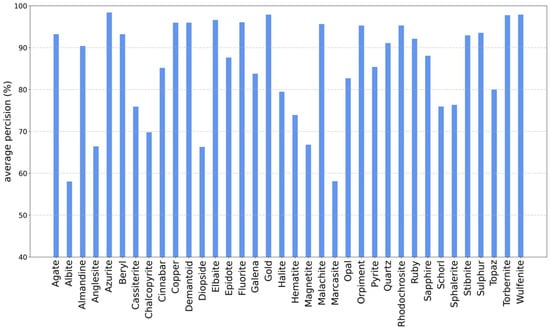
Figure 5.
The average precision (AP) of each mineral for the model of the paper.
4.2.4. Visualization of the Class Activation Mapping
In order to understand which areas the model pays attention to when making predictions on associated mineral images, Grad-CAM [32] is used to visualize the feature extraction results obtained in the Part 1 of the model. Grad-CAM can figure out which areas the model is focusing on and is now widely used to evaluate the performance of the feature extraction [32]. In order to meet the requirement of the input of the Grad-CAM, the feature extraction matrix obtained in the Part 1 of our model is reshaped from to .
Three activation maps of associated minerals are shown in Figure 6. In Figure 6, the first column is the original mineral image, the second (third, fourth) column is where the model focuses on when it identifies the minerals. From Figure 6 we can see that our model has a good feature extraction ability and can locate the identified minerals roughly.
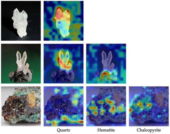
Figure 6.
Class activation maps of three associated minerals based on Grad-CAM. The first column is the original mineral image, and the remaining columns are the Grad-CAM visualization results of a certain mineral.
4.2.5. Comparison with Other Mineral Identification Methods
As stated in Section 1, there has been a lot of work using deep learning to identify a single mineral in an image no matter how many minerals exist in the image, for example the work [4,5,6,7,8,9,10]. To enable the models of those work identify multiple minerals in an image, the output layer of the models can be changed from the function softmax to the function sigmoid. The model of research [10] has the highest performance among the previous work, so its output layer was changed from the function softmax to the function sigmoid to compare with our model. The modified model of research [10] was trained and tested on the same data as ours. The comparison results are shown in Table 5. It can be seen from Table 5 that our model has higher mAP than the model modified from the best single mineral identification model.
Table 5.
Comparison results of our model and the modified model of research [10] on our dataset.
5. Conclusions
In this paper, a model that can identify multiple minerals in an image was proposed, which uses the transformer architecture and the multi-label classification method for mineral identification. Through the attention mechanism in the transformer decoder, this model can quickly and accurately identify all minerals that exist in the image using only the image of the mineral as input. Compared with the traditional methods based on the physical and chemical characteristics of minerals, the model proposed in this paper can accurately identify minerals without requiring mineral expertise, which greatly saves manpower. Compared to other machine learning or deep learning methods that can only identify a single mineral in an image, our method can identify multiple minerals in an image. Of the 183,688 images datasets of 36 common minerals, the experimental results show that our model can achieve a mean average precision of 85.26% and can roughly locate the identified minerals. In the future, more mineral data will be collected to identify more categories of minerals and other deep learning methods will be used to accurately locate all the minerals in the image.
Author Contributions
Conceptualization, X.J., M.Y., M.H., Z.Z. and X.Z.; methodology, X.J., B.W., Y.C. and Y.W.; software, B.W.; validation, M.Y., M.H., Z.Z. and X.Z.; writing—original draft preparation, B.W.; writing—review and editing, X.J. and Z.Z. All authors have read and agreed to the published version of the manuscript.
Funding
This research was funded by the Program of National Mineral Rock and Fossil Specimens Resource Center from MOST and Major Science and Technology Projects of PetroChina Southwest Oil & Gasfield Company (No.2019ZD01).
Data Availability Statement
Data sharing is not applicable.
Acknowledgments
The authors are grateful to the provision of mineral images from National Mineral Rock and Fossil Specimens Resource Center from MOST and mindat.org. The authors are also grateful to the anonymous reviewers for their constructive comments, which have significantly raised the quality of the manuscript and enabled us to improve the manuscript. Special thanks are given to the editors, for their kind patience and encouragements in revising the manuscript.
Conflicts of Interest
The authors declare no conflict of interest.
References
- Lou, W.; Zhang, D.; Bayless, R.C. Review of mineral recognition and its future. Appl. Geochem. 2020, 122, 104727. [Google Scholar] [CrossRef]
- Hao, H.; Gu, Q.; Hu, X. Research Advances and Prospective in Mineral Intelligent Identification Based on Machine Learning. Earth Sci. 2021, 46, 3091–3106. [Google Scholar] [CrossRef]
- LeCun, Y.; Bengio, Y.; Hinton, G. Deep learning. Nature 2015, 521, 436–444. [Google Scholar] [CrossRef] [PubMed]
- Zeng, X.; Xiao, Y.; Ji, X.; Wang, G. Mineral Identification Based on Deep Learning That Combines Image and Mohs Hardness. Minerals 2021, 11, 506. [Google Scholar] [CrossRef]
- Peng, W.H.; Bai, L.; Shang, S.W.; Tang, X.J.; Zhang, Z.Y. Common mineral intelligent recognition based on improved InceptionV3. Geol. Bull. China 2019, 38, 2059–2066. [Google Scholar] [CrossRef]
- Liu, C.; Li, M.; Zhang, Y.; Han, S.; Zhu, Y. An Enhanced Rock Mineral Recognition Method Integrating a Deep Learning Model and Clustering Algorithm. Minerals 2019, 9, 516. [Google Scholar] [CrossRef]
- Brempong, E.A.; Agangiba, M.; Aikins, D. MiNet: A Convolutional Neural Network for Identifying and Categorising Minerals. Ghana J. Technol. 2020, 5, 86–92. [Google Scholar] [CrossRef]
- Guo, Y.; Zhou, Z.; Lin, H.; Liu, X.; Chen, D.; Zhu, J.; Wu, J. The mineral intelligence identification method based on deep learning algorithms. Earth Sci. Front. 2020, 27, 39–47. [Google Scholar] [CrossRef]
- Li, M.; Liu, C.; Zhang, Y. A Deep Learning and Intelligent Recognition Method of Image Data for Rock Mineral and its Implementation. Geotecton. Miner. 2020, 44, 203–211. [Google Scholar]
- Jia, L.; Yang, M.; Meng, F.; He, M.; Liu, H. Mineral Photos Recognition Based on Feature Fusion and Online Hard Sample Mining. Minerals 2021, 11, 1354. [Google Scholar] [CrossRef]
- Tsoumakas, G.; Katakis, I. Multi-Label Classification: An Overview. Int. J. Data Warehous. Min. 2009, 3, 1–13. [Google Scholar] [CrossRef]
- Tarekegn, A.N.; Giacobini, M.; Michalak, K. A review of methods for imbalanced multi-label classification. Pattern Recognit. 2021, 118, 107965. [Google Scholar] [CrossRef]
- Zhang, M.; Zhou, Z. A Review on Multi-Label Learning Algorithms. IEEE Trans. Knowl. Data Eng. 2014, 26, 1819–1837. [Google Scholar] [CrossRef]
- Wei, Y.; Xia, W.; Lin, M.; Huang, J.; Ni, B.; Dong, J.; Zhao, Y.; Yan, S. HCP: A Flexible CNN Framework for Multi-Label Image Classification. IEEE Trans. Softw. Eng. 2016, 38, 1901–1907. [Google Scholar] [CrossRef] [PubMed]
- Lin, W.-Z.; Fang, J.-A.; Xiao, X.; Chou, K.-C. iLoc-Animal: A multi-label learning classifier for predicting subcellular localization of animal proteins. Mol. BioSystems 2013, 9, 634–644. [Google Scholar] [CrossRef] [PubMed]
- Xiao, X.; Wu, Z.-C.; Chou, K.-C. iLoc-Virus: A multi-label learning classifier for identifying the subcellular localization of virus proteins with both single and multiple sites. J. Theor. Biol. 2011, 284, 42–51. [Google Scholar] [CrossRef] [PubMed]
- Salvatore, C.; Castiglioni, I. A Wrapped Multi-label Classifier for the Automatic Diagnosis and Prognosis of Alzheimer’s Disease. J. Neurosci. Methods 2018, 302, 58–65. [Google Scholar] [CrossRef] [PubMed]
- Shao, Z.; Zhou, W.; Deng, X.; Zhang, M.; Cheng, Q. Multilabel remote sensing image retrieval based on fully convolutional network. IEEE J. Sel. Top. Appl. Earth Obs. Remote Sens. 2020, 13, 318–328. [Google Scholar] [CrossRef]
- A Mineral Database. Available online: https://www.mindat.org/ (accessed on 20 July 2022).
- He, K.; Zhang, X.; Ren, S.; Sun, J. Deep Residual Learning for Image Recognition. In Proceedings of the 2016 IEEE Conference on Computer Vision and Pattern Recognition(CVPR), Las Vegas, NV, USA, 16 June–1 July 2016; pp. 770–778. [Google Scholar]
- Sandler, M.; Howard, A.; Zhu, M.; Zhmoginov, A.; Chen, L.C. MobileNetV2: Inverted Residuals and Linear Bottlenecks. In Proceedings of the 2018 IEEE/CVF Conference on Computer Vision and Pattern Recognition (CVPR), Salt Lake City, UT, USA, 18–23 June 2018; pp. 4510–4520. [Google Scholar] [CrossRef]
- Kolesnikov, A.; Beyer, L.; Zhai, X.; Puigcerver, J.; Yung, J.; Gelly, S.; Houlsby, N. Big Transfer (BiT): General Visual Representation Learning. In Proceedings of the 2020 ECCV European Conference on Computer Vision, Lecture Notes in Computer Science; Springer: Cham, Switzerland, 2007; Volume 12350, pp. 491–507. [Google Scholar] [CrossRef]
- Dosovitskiy, A.; Beyer, L.; Kolesnikov, A.; Weissenborn, D.; Zhai, X.; Unterthiner, T.; Dehghani, M.; Minderer, M.; Heigold, G.; Gelly, S. An image is worth 16x16 words: Transformers for image recognition at scale. In Proceedings of the 2021 The International Conference on Learning Representations (ICLR), Online, 4–8 May 2021. [Google Scholar] [CrossRef]
- Vaswani, A.; Shazeer, N.; Parmar, N.; Uszkoreit, J.; Jones, L.; Gomez, A.N.; Kaiser, Ł.; Polosukhin, I. Attention is all you need. In Proceedings of the 31st Annual Conference on Neural Information Processing Systems (NIPS), Long Beach, CA, USA, 4–9 December 2017. [Google Scholar] [CrossRef]
- Ba, J.L.; Kiros, J.R.; Hinton, G.E. Layer Normalization. arXiv 2016, arXiv:1607.06450. [Google Scholar] [CrossRef]
- Carion, N.; Massa, F.; Synnaeve, G.; Usunier, N.; Kirillov, A.; Zagoruyko, S. End-to-end object detection with transformers. In Proceedings of the 2020 ECCV European Conference on Computer Vision, Online, 23–28 August 2020; pp. 213–229. [Google Scholar] [CrossRef]
- Ben-Baruch, E.; Ridnik, T.; Zamir, N.; Noy, A.; Zelnik-Manor, L. Asymmetric Loss For Multi-Label Classification. In Proceedings of the 2021 IEEE International Conference on Computer Vision(ICCV), Montreal, BC, Canada, 11–17 October 2021; pp. 82–91. [Google Scholar] [CrossRef]
- Lin, T.Y.; Goyal, P.; Girshick, R.; He, K.; Dollár, P. Focal Loss for Dense Object Detection. In Proceedings of the IEEE International Conference on Computer Vision(ICCV), Venice, Italy, 22–29 October 2017; pp. 2999–3007. [Google Scholar] [CrossRef]
- Loshchilov, I.; Hutter, F. Decoupled weight decay regularization. In Proceedings of the 2019 The International Conference on Learning Representations (ICLR), New Orleans, LA, USA, 6–9 May 2019. [Google Scholar] [CrossRef]
- Cubuk, E.D.; Zoph, B.; Shlens, J.; Le, Q.V. Randaugment: Practical automated data augmentation with a reduced search space. In Proceedings of the 2020 IEEE Conference on Computer Vision and Pattern Recognition(CVPR), Seattle, WA, USA, 14–19 June 2020; pp. 702–703. [Google Scholar]
- Liu, Z.; Lin, Y.; Cao, Y.; Hu, H.; Wei, Y.; Zhang, Z.; Lin, S.; Guo, B. Swin transformer: Hierarchical vision transformer using shifted windows. In Proceedings of the IEEE/CVF International Conference on Computer Vision(ICCV), Montreal, BC, Canada, 11–17 October 2021; pp. 10012–10022. [Google Scholar] [CrossRef]
- Selvaraju, R.R.; Cogswell, M.; Das, A.; Vedantam, R.; Parikh, D.; Batra, D. Grad-cam: Visual explanations from deep networks via gradient-based localization. In Proceedings of the IEEE International Conference on Computer Vision(ICCV), Venice, Italy, 22–29 October 2017; pp. 618–626. [Google Scholar]
Publisher’s Note: MDPI stays neutral with regard to jurisdictional claims in published maps and institutional affiliations. |
© 2022 by the authors. Licensee MDPI, Basel, Switzerland. This article is an open access article distributed under the terms and conditions of the Creative Commons Attribution (CC BY) license (https://creativecommons.org/licenses/by/4.0/).