Gravity Data Reveal New Evidence of an Axial Magma Chamber Beneath Segment 27 in the Southwest Indian Ridge

Abstract

Hydrothermal systems are integral to mid-ocean ridge activity; they form massive seafloor sulfide (SMS) deposits rich in various metallic elements, which are potential mineral resources. Since 2007, many hydrothermal fields have been discovered along the ultraslow-spreading Southwest Indian Ridge (SWIR). The Duanqiao hydrothermal field is located at segment 27’s axis between the Indomed and Gallieni transform faults; tomography models reveal an obvious low-velocity anomaly beneath it, indicating a possible axial magma chamber (AMC). However, confirmation of an AMC’s existence requires further study and evidence. In this study, we first calculated the gravity effect to identify the heterogeneous distribution of crustal density beneath segment 27 and the surrounding area. Next, we used the gravity-inversion method to obtain the crustal density structure beneath the study area. The results indicate that a thickened crust and low-density crustal materials exist beneath segment 27. The low-density anomaly in the lower crust beneath the Duanqiao hydrothermal field suggests the existence of an AMC covered with a cold and dense upper crust. The density results identify several faults, which provide potential channels for magma migration. In addition, the melt migrates westward and redistributes laterally toward the segment’s western end. However, when migrating toward the segment’s eastern end, the melt is affected by a rapid cooling mechanism. Therefore, the segment’s ends present different density features and morphologies of nontransform discontinuities (NTDs).

1. Introduction

The mid-ocean ridge is a spreading boundary in plate tectonic theory and a significant channel for studying the Earth’s interior and deep activities. Hydrothermal systems are important components of mid-ocean ridge activity; they are influenced by magmatism, tectonism [1], and biogeochemistry [2]. A comprehensive study method on the seafloor hydrothermal system was firstly constructed in the Salton Sea by geological, geophysical, and thermal data [3]. The heat flux from seafloor hydrothermal systems accounts for 20% to 25% of the total global heat flux. The polymetallic sulfide formed by the mid-ocean ridge’s hydrothermal system is rich in multiple metallic elements [4] and will become a significant domain for resource exploration. More than half of global seafloor hydrothermal fields are located on the mid-ocean ridge, mostly on the East Pacific Rise (EPR) and Mid-Atlantic Ridge (MAR). The extensive investigation of these ridges includes studies of the TAG [5], Rainbow [6], Lost City [7], and Logatchev [8] hydrothermal fields.

The hydrothermal systems of ultraslow-spreading ridges are characterized by a deep thermal source and hydrothermal circulation [9]; they have not been as extensively investigated [10] as fast- and slow-spreading ridges. As the largest and most completely developed ultraslow-spreading ridge, the Southwest Indian Ridge (SWIR) has complex structural characteristics, special crustal accretion patterns, and frequent hydrothermal activities. Therefore, several China DAYANG cruises have been organized to investigate and study the SWIR’s hydrothermal activities. In 2007, the first active hydrothermal field (Longqi hydrothermal field) was discovered off the SWIR at 49°39′ E, 37°47′ S by D/V Dayang Yihao using water column surveys, deep-tow video imaging, and an autonomous benthic explorer (ABE) [11]. Subsequently, seismic data were collected using ocean bottom seismometers (OBSs), which provide images of the velocity structure beneath segments 27, 28, and 29. Velocity variation confirms the existence of a detachment fault [12] near the Longqi hydrothermal field that has a penetration depth deeper than the fault near the TAG hydrothermal field [13]. In addition, recent research analyzed deep hydrothermal circulation in a detachment faulting system on the ultraslow-spreading ridge using different methods [14,15,16]. Segment 27 includes the inactive Duanqiao hydrothermal field [4,11] and several hydrothermal plume anomalies [17,18]. The velocity structure obtained using wide-angle seismic reflection data from OBS indicates different lateral velocity variations and crust thicknesses beneath segments 27 to 29 [19]. The thickened crust beneath segment 27 reveals the existence of a high-temperature mantle and enriched melt. To confirm the existence of melt beneath segment 27, a seismic tomography model of the crust beneath segment 27 was constructed using OBS data, which revealed an anomalously thick crust of about 10 km and a low-velocity anomaly of −0.6 km/s [19,20,21] in the lower crust beneath the central volcanoes. This model also confirms the existence of an axial magma chamber (AMC) beneath segment 27 [22].

In this study, we first determined the gravity effect to identify the heterogeneous distribution of crustal density beneath segment 27 and the surrounding area through various corrections to and processing of the original ship-borne gravity and multi-beam bathymetry data. Next, we constructed a model of the crustal density structure beneath segment 27 using the three-dimensional gravity inversion method to discuss the heterogeneous distribution characteristics of crustal density and their geological implications. Finally, we provide gravity evidence to confirm the existence of an AMC beneath segment 27.

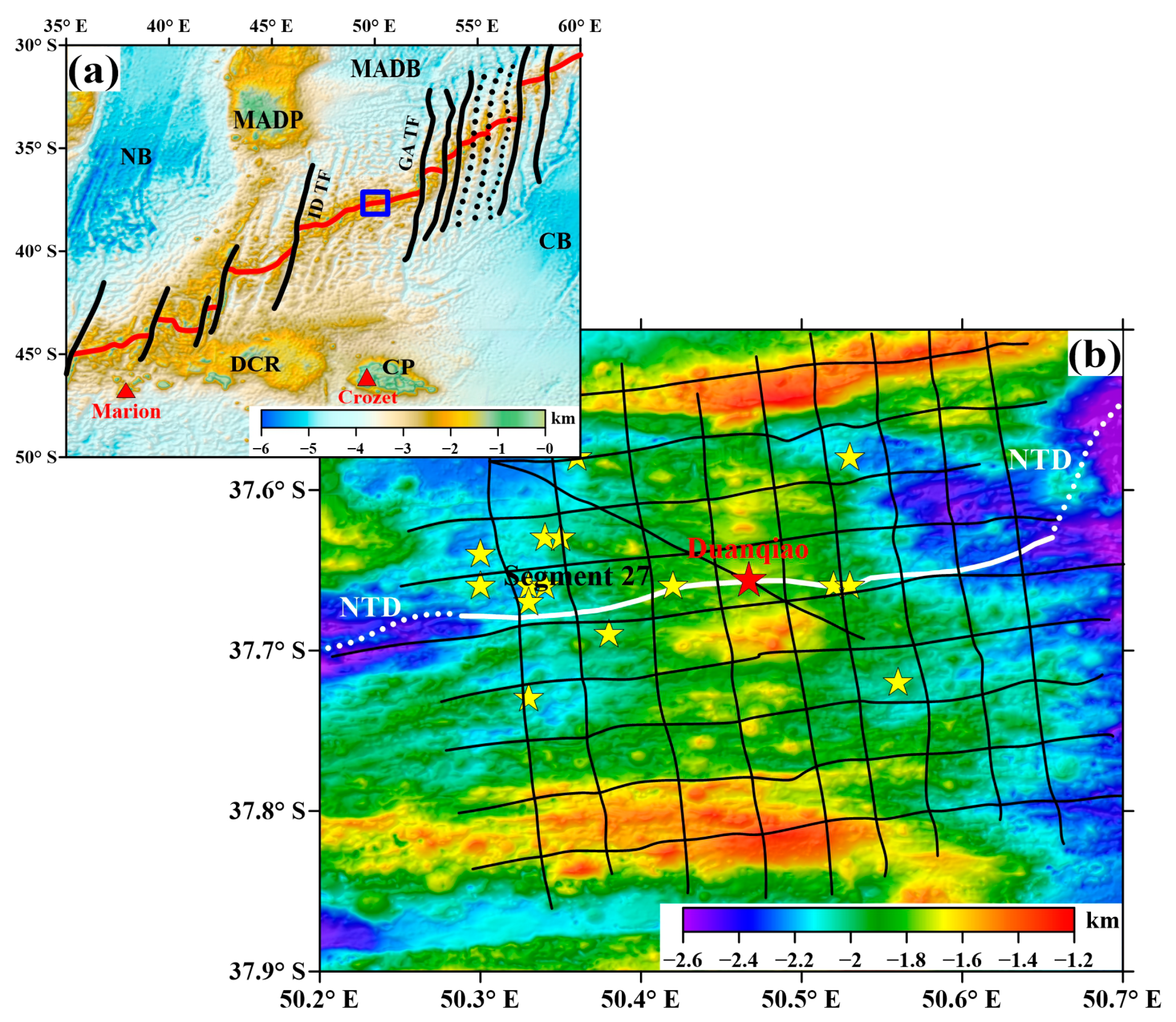
2. Geological Background

The SWIR extends east to west from the Rodrigues Triple Junction (RTJ) to the Bouvet Triple Junction (BTJ) and is approximately 8000 km long. It is a significant boundary between the African and Antarctic plates [4]. It belongs to an ultraslow-spreading ridge with an approximate spreading rate of 1.4~1.6 cm/a. Some segments are characterized by a high degree of oblique spreading, including the western segment, which spreads at a slightly faster rate than the eastern segment [23,24]; there is little variation in the spreading rate along the ridge axis [25]. Topographic and geophysical data indicate an obvious difference in the central rift morphology [26,27], topographic characteristics [28], crust thickness [29], magmatic activity [30,31], and mantle composition [32,33] along the SWIR from the BTJ to the RTJ. The ridge’s axis is segmented by a series of N–S transform faults (Figure 1a). The basement rocks consist mainly of basalts, peridotites, and gabbros, with serpentinized peridotites exposed near transform fault areas and gabbros exposed near large fault areas [34,35].

The SWIR segment between the Indomed (ID) and Gallieni (GA) transform faults (TFs) has been investigated more than others. The bathymetry of the axial rift is relatively shallow and even disappears in some areas, with a relatively thick oceanic crust and enriched magma supply [19,37,38]. Related studies attribute this segment’s unique phenomenon to the interaction between the Crozet hotspot and the SWIR [38,39,40,41]. The Duanqiao hydrothermal field is in the high relief area (Figure 1b) in segment 27’s axial volcanic ridge (AVR) between the ID and GA TFs. The bathymetry is approximately 1700 m with densely distributed seamounts and axial volcanoes [4,42]. The surrounding terrain is smooth. Previous research suggests that segment 27’s low mantle Bouguer gravity anomaly (MBA) and Na_8.0 content value indicate a thickened oceanic crust and relatively robust melt supply [37]. However, no temperature or turbidity anomalies were reported, which indicates that the Duanqiao hydrothermal field is currently inactive [4].

3. Data and Methods

3.1. Gravity Data

In this study, gravity and bathymetry data were derived using ship-borne gravity and multi-beam seafloor topography data collected by the 30th China DAYANG cruise in the SWIR segment between the ID and GA TFs, including four navigation sections during six months. The L&R S II-162 air–sea gravimeter (LaCoste Romberg Company, Lafayette, CO, USA) was used for measurement of gravity data during this cruise. It is one of the most advanced ocean gravimeters with measurement accuracy of 1 mGal, static sensitivity of 0.01 mGal, measurement range of 12000 mGal, and linear drift of less than 3 mGal/month. The maximum operating angle of the gyro-stabilized platform is ± 25°. The navigation measurement method was used for the collection of gravity data. Surveyed lines are shown in Figure 1b as solid black lines. In every surveyed line, the resolution of original ship-borne gravity and multi-beam seafloor topography data was 100 m. The free air gravity anomaly was obtained via zero-drift correction, draft correction, Eötvös correction, normal field correction, and free air correction on the original gravity data [42].

Next, we used the Kriging method to remesh a 500 m × 500 m data grid. The simple Bouguer gravity anomaly is calculated by Bouguer correction on the free air gravity anomaly. The complete Bouguer gravity anomaly is usually calculated by both Bouguer correction and terrain correction on the free air gravity anomaly. However, ref. [43] suggested the Bouguer correction has not been made in a “free air” map on the ocean. In this study, we used the generalized terrain correction method (also called external correction). The generalized terrain correction is based on the reference ellipsoid to calculate the influence of the global continent and seafloor topography on the gravity value. It integrates the Bouguer correction and the terrain correction into a whole. For marine gravity, the generalized terrain correction is more simple, convenient, practical, and feasible than the separate Bouguer correction and terrain correction [44]. For the generalized terrain correction, the terrain correction range is divided into near, junction, and far zones [45].

The near and junction zone’s range is 0 to 50 (or 100) m and 50 (or 100) to 2000 m, respectively, and the terrain correction was calculated using the upright prismatic formula [46]. As shown in Figure 2a, the terrain of the near and junction zones is assumed to be an upright prism with a bottom surface of 100 m × 100 m and a height of the average bathymetry of four corner points. Taking the measurement point as the origin, the gravity effect value of the prism on the measurement point is deduced. As shown in Figure 2b, assuming that the residual density of the upright prism is ρ, the gravity anomaly at the origin of coordinates is

$$\begin{array}{l}\Delta g=G\rho {\left|{\left|{\left|x\ln (y+r)+y\ln (x+r)-z\cdot \arctan (\frac{xy}{zr})\right|}_{x_1}^{x_2}\right|}_{y_1}^{y_2}\right|}_{z_1}^{z_2}\\ r=\sqrt{x^2+y^2+z^2}\end{array}$$

(1)

where G is the gravitational constant (6.67 × 10⁻¹¹ m³/(kg·s²)), ρ denotes the density of terrain correction (1.64 g/cm³), and r is the distance between the calculated and measurement points (in m).

The far zone is further divided into first and second far zones [45]. The first and second far zone’s range is 2 to 20 km and 20 to 166.7 km, respectively, and the terrain correction was calculated using the spherical coordinate method [47]. As shown in Figure 3, the terrain correction in a single ring can be calculated using

$$\Delta g=G\rho {\displaystyle {\int }_0^h{\displaystyle {\int }_{\theta 1}^{\theta 2}{\displaystyle {\int }_0^{2\pi }\frac{(R+Z)-(R+h)\cos \theta }{{\left[{(R+Z)}^2+{(R+h)}^2-2(R+Z)(R+h)\cos \theta \right]}^{\raisebox{1ex}{$3$}\!\left/ \!\raisebox{-1ex}{$2$}\right.}}\times {(R+h)}^2\sin \theta d\varphi d\theta dh}}}$$

(2)

where G is the gravitational constant (6.67 × 10⁻¹¹ m³/(kg·s²)), ρ is the average crustal density (2.67 g/cm³), R is the average radius of the Earth (6371.025 km), Z is the elevation of calculated points (in m), and h is the average elevation of ring (in m).

In all calculations, we used a seawater density of 1.03 g/cm³ and an oceanic crustal density of 2.67 g/cm³. As seen in Figure 4a, segment 27, where the Duanqiao hydrothermal field is located, has a relatively high free air gravity anomaly value compared to the NTD on both of segment 27’s flanks, reflecting the topographic contrast between the axial volcano and axial valley. High free air gravity anomaly values on both the north and south sides, away from segment 27’s axis, indicate the existence of high topographic structures. Following this, we removed the gravity effect of terrain from the free air gravity anomaly to obtain the complete Bouguer gravity anomaly. Figure 4b illustrates a high positive Bouguer gravity anomaly value in most of the study area. Specifically, the Bouguer gravity anomaly value is lower in segment 27 compared to NTDs. The Duanqiao hydrothermal field and the areas surrounding it have the lowest Bouguer gravity anomaly values. The areas to the north and south, away from segment 27’s axis, have a low Bouguer gravity anomaly with an almost symmetric distribution center on the axis.

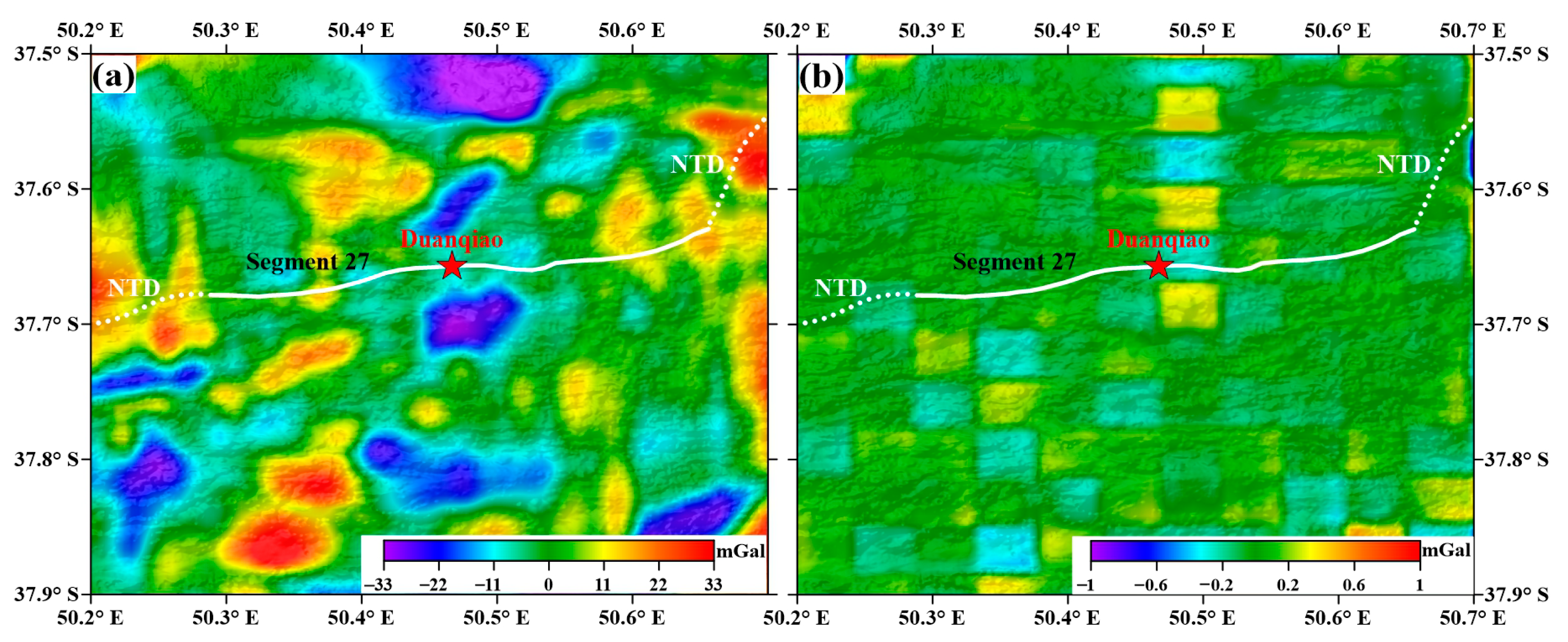
3.2. Anomaly Separation

The Bouguer gravity anomaly reflects the density contrast between subsurface materials and normal earth. Matched filtering technology has been widely used to process gravity and magnetic data to separate the deep and shallow source fields [48]. In this study, the matched filtering method was used to separate the shallow source field from the Bouguer gravity anomaly. The shallow source field anomaly is regarded as a gravity anomaly that can reflect the heterogeneous distribution of crustal density; it was used in the crustal density structure imaging in the study area. The radial logarithmic power spectrum of the Bouguer gravity anomaly is shown in Figure 5a. Figure 5b shows the low value of the shallow source anomaly in the Duanqiao hydrothermal field and the surrounding area.

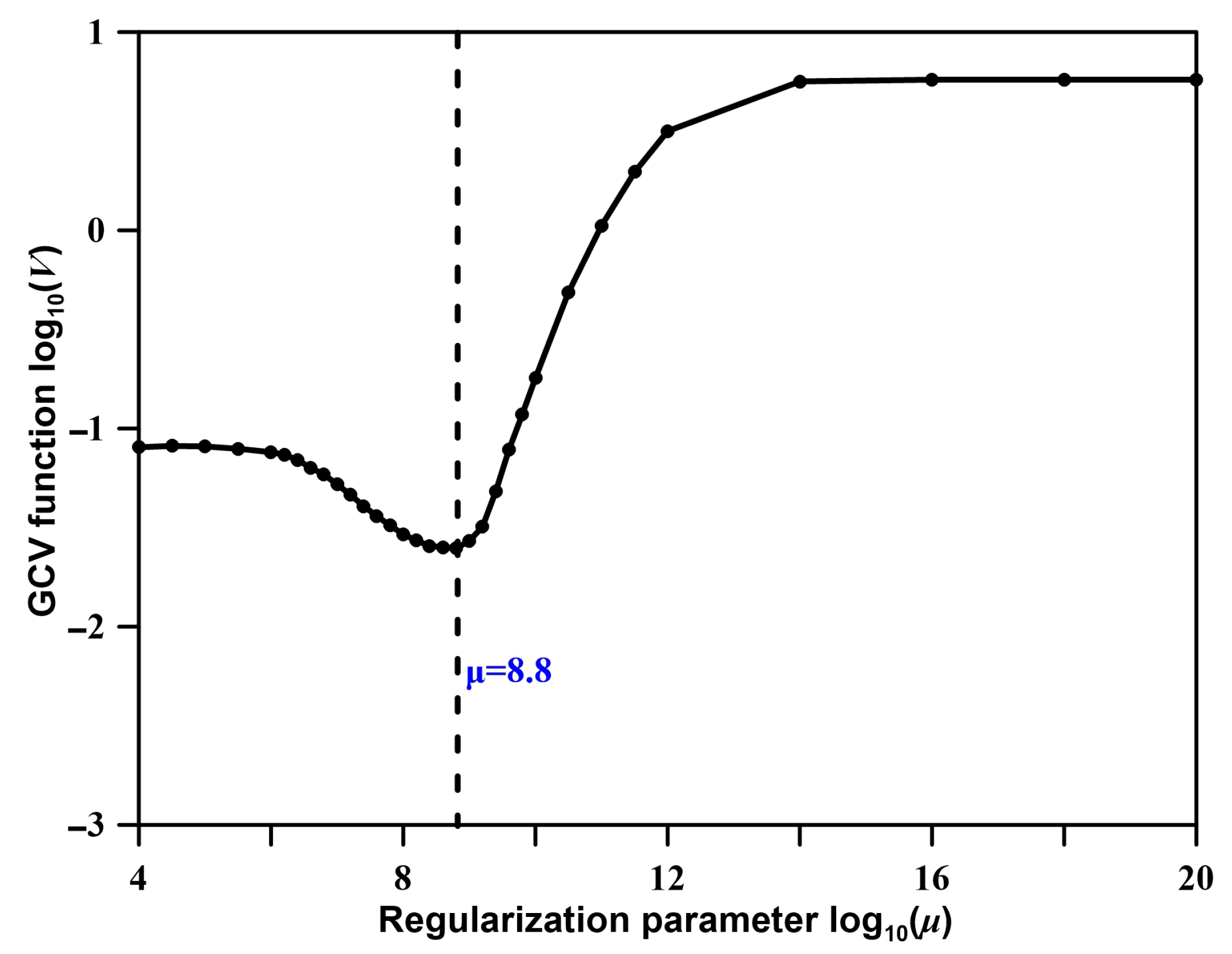
3.3. Inversion Method

According to [49]’s proposal, we added a model objective function to solve the optimization problem [50,51]. The total objective function of the inversion Φ is defined as

$$\mathsf{\Phi }={\mathsf{\Phi }}_d+\mu {\mathsf{\Phi }}_m$$

(3)

where Φ_d is the data misfit, Φ_m denotes the model objective function, and μ is the balance factor (also called the regularization parameter) that determines the trade-off between the two objective functions. Φ_d and Φ_m can be expressed in matrix form as follows

$${\mathsf{\Phi }}_d={\Vert {\mathrm{W}}_d(\mathrm{G}m-d^{obs})\Vert }^2,{\mathsf{\Phi }}_m={\Vert {\mathrm{W}}_m(m-m_{ref})\Vert }^2$$

(4)

where G is the kernel matrix or the integral operator for converting the density into the gravity field; W_d is the diagonal matrix; W_m is the weighting matrix, one of the most important parameters in the model objective function; d^obs is observed data; and m and m_ref represent the pending density and reference (or initial) density vectors, respectively. Therefore, the final inversion objective function is converted as

$$\mathsf{\Phi }={\Vert {\mathrm{W}}_d(\mathrm{G}m-d^{obs})\Vert }^2+\mu {\Vert {\mathrm{W}}_m(m-m_{ref})\Vert }^2$$

(5)

after which we take the derivative of m using Equation (5), obtaining

$$({\mathrm{G}}^T{\mathrm{W}}_d^T{\mathrm{W}}_d\mathrm{G}+\mu {\mathrm{W}}_m^T{\mathrm{W}}_m)m={\mathrm{G}}^T{\mathrm{W}}_d^T{\mathrm{W}}_d{d}^{obs}+\mu {\mathrm{W}}_m^T{\mathrm{W}}_m{m}_{ref}$$

(6)

and use the conjugate gradient method to resolve Equation (6) in the actual inversion application process.

Next, we use the generalized cross-validation (GCV) method [52,53,54] to choose a suitable regularization parameter. Using GCV in inverse problems with inequality constraints, such as positivity, requires solving a number of auxiliary optimization problems, which in turn requires a significant amount of computation. If no other information is available, the value of µ obtained in this manner can be used directly in the final inversion that has positivity imposed. In this case, only one logarithmic barrier solution is required. Numerical tests indicate that this simplistic use of GCV is, in fact, surprisingly effective unless the data have a large negative bias or are distributed too sparsely [52]. Therefore, the GCV curve is obtained using the relationship between different μ and the corresponding correlation functions V(μ) as

$$V(\mu )=\frac{{\Vert {\mathrm{W}}_d(\mathrm{G}m-d^{obs})-{\mathrm{W}}_d{\mathrm{JM}}^{-1}\mathrm{B}\Vert }^2}{{[N-\mathrm{trace}({\mathrm{W}}_d{\mathrm{JM}}^{-1}{\mathrm{J}}^T{\mathrm{W}}_d^T)]}^2}$$

(7)

where the implication in Equation (7) is same as above, N is the number of data; and trace represents the matrix trace operation. Meanwhile,

$$\mathrm{M}={\mathrm{J}}^T{\mathrm{W}}_d^T{\mathrm{R}}_d{\mathrm{W}}_d\mathrm{J}+\mu {\mathrm{W}}_m^T{\mathrm{R}}_m{\mathrm{W}}_m$$

(8)

$$\mathrm{B}={\mathrm{J}}^T{\mathrm{W}}_d^T{\mathrm{R}}_d{\mathrm{W}}_d(\mathrm{G}m-d^{obs})+\mu {\mathrm{W}}_m^T{\mathrm{R}}_m{\mathrm{W}}_m(m-m_{ref})$$

(9)

where J is the Jacobian matrix; R_d and R_m represent the diagonal matrix of Φ_d and Φ_m, respectively, whose diagonal elements are determined by the choice of general measures [55,56]. In general, the inflection point of the GCV curve is chosen as the suitable regularization parameter.

In this study, we did not use a seismic tomography model or other data as our initial density model in the process of gravity inversion because we hoped the AMC could be presented only using gravity data. The constrained model is the smoothest model. We need to set the inversion parameters. The inversion area is segment 27, and the surrounding area in the SWIR is between 50.2° E and 50.7° E and between 37.9° S and 37.5° S. The depth ranges from 0 to 18 km. The lateral and vertical grid sizes are 0.5 km and 1 km, respectively. We consider the inversion result of the regularization parameter at the inflection point (μ = 8.8) of the GCV curve (Figure 6) to be the final result.

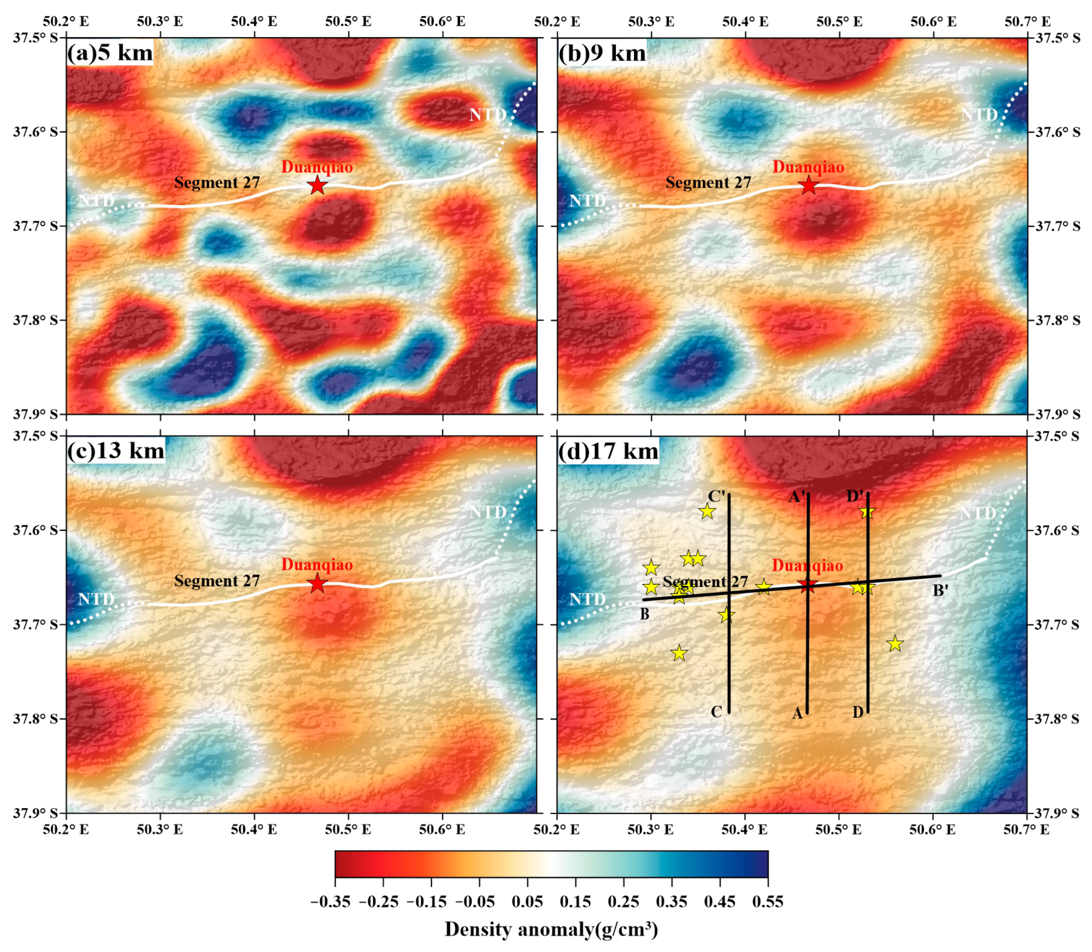
4. Inversion Results

We obtained the final density anomaly imaging result using the inversion method noted above, with appropriate parameters. The inverted density model produces the predicted gravity anomalies, which are very close to the observed gravity data with data misfit ± 1 mGal (Figure 7).

The inverted density model demonstrates the three-dimensional density variation in the observed gravity anomaly (Figure 5b). In Figure 8, we present slices of lateral density anomaly distribution at depths of 5 km, 9 km, 13 km, and 17 km. At 5 km deep, the density anomaly’s amplitude is large. A low-density anomaly and a high-density anomaly appear beneath both the south and north sides of segment 27’s axis. In addition, high-density anomaly characteristics start to appear beneath NTDs on segment 27’s west and east flanks (Figure 8a). As depth increases from 5 to 9 km, a low-density anomaly starts to appear beneath the Duanqiao hydrothermal field, reaching a minimum value of −0.2 g/cm³ at 9 km (Figure 8b). High-density anomalies beneath NTDs also reach the maximum at this depth. In this depth range, areas with low- and high-density anomalies are distributed at intervals on segment 27’s axis. As depth increases from 13 to 17 km in the uppermost mantle, the low-density anomaly characteristic beneath the Duanqiao hydrothermal field starts to weaken (Figure 8c). Similarly, the density anomaly characteristics beneath other areas weaken as depth increases, and the western NTD retains a high-density anomaly at 17 km (Figure 8d). In general, the study area presents a variation in density with depth beneath different areas. Density anomaly variation characteristics are more obvious in the crust than they are in the upper mantle.

5. Discussion

5.1. Artifacts in the Data Misfit

The data misfit is less than 1 mGal between the observed and predicted gravity data, indicating the data can be fitted well. However, the ~5 km-large artifacts are shown in the data misfit (Figure 7b), which are not consistent with the 0.5 km-large horizontal inversion cell. We consider these ~5 km-large artifacts are probably from the originally collected data. Although the interval of measure point in every line is 100 m, the interval of surveyed lines is relatively large and approaches 5 km, as shown in Figure 1b. Therefore, in the collection of ship-borne gravity and multi-beam bathymetry data, the interval between surveyed lines should also be considered. Reducing the interval between surveyed lines can not only improve the data resolution but also make the subsequent data processing and calculation more reliable.

5.2. Heterogeneous Distribution of Crustal Density and Its Implications

In general, gravity-inversion results indicate that segment 27 has low-density anomaly characteristics and that high-density anomaly characteristics occur beneath NTDs, which correspond to the shallow source field anomaly (Figure 5b) that was identified using matched filtering on the Bouguer gravity anomaly, indicating the heterogeneous lateral distribution of crustal density beneath segment 27 and the surrounding area. Different tectonic units also have different density anomaly variation characteristics at different depths, indicating the vertical heterogeneous distribution of crustal density beneath the study area.

In a given region, a low Bouguer gravity anomaly value can indicate a relatively thickened crust compared with a normal crust, or a decrease in density. The Bouguer gravity anomaly (Figure 4b) indicates that segment 27, especially the Duanqiao hydrothermal field, has the most obvious low Bouguer gravity anomaly; this possibly indicates a thickened crust beneath segment 27, which is consistent with the seismic imaging results [19]. The gravity inversion results demonstrate that there is a deep low-density anomaly beneath the Duanqiao hydrothermal field and the surrounding area, indicating that a low Bouguer gravity anomaly value is possibly an effect of a thickened crust and low-density materials. Figure 9 shows four extracted density anomaly profiles with cross-sections AA′, CC′, and DD′ across segment 27’s axis and BB′ along segment 27’s axis. The AA′ profile (Figure 9a) suggests that the Duanqiao hydrothermal field has a low-density anomaly in its lower crust, indicating the existence of melts, whereas its upper crust shows no obvious low-density anomaly features. Meanwhile, low- and high-density anomalies both north and south of segment 27 are alternately distributed, centered on the axis of profile AA′. This corresponds with the lateral density anomaly slices at depths of 5 to 9 km, which reveal a multi-period topographic difference formed by the ridge’s symmetric spreading. Such symmetric topographic and density features can also reflect the crustal accretion pattern of a ridge. During the process of mid-ocean ridge spreading to form a new oceanic crust, the older oceanic crust is pushed away from the spreading center. A similar symmetric feature is also shown in magnetic anomaly [57] and crustal age [58].

Figure 9c also illustrates a similar density anomaly. The AA′ and CC′ profiles present different density features beneath segment 27’s axis in the upper crust. The profile of CC′ shows low density beneath segment 27’s axis, whereas the Duanqiao hydrothermal field presents high density at shallow depths. Moreover, many boundaries between low- and high-density anomalies are evident in both profiles. Such boundaries indicate the probable existence of massive fault structures, which can provide channels for magma migration. In addition, density anomalies primarily accumulate in the crust, whereas the amplitude is relatively low in the upper mantle, indicating that the crust is more heterogeneous than the upper mantle.

5.3. Axial Magma Chamber beneath Segment 27

The segment between the ID and GA TFs has a thicker crust compared with other SWIR segments [38,59]. SWIR segments 27, 28, and 29 have been extensively investigated. China’s DAYANG cruises have already discovered Duanqiao, Longqi, and Yuhuang hydrothermal fields, at the axis or surrounding areas of the segments, respectively. Unlike segments 28 and 29, segment 27 is characterized by a shallow average bathymetry and a dense distribution of axial seamounts and volcanoes. Low MBA and Na_8.0 contents indicate a relatively thick crust and robust melt supply beneath segment 27 [37]. The velocity structure obtained using OBS wide-angle seismic reflection data confirms the existence of thickened oceanic crust [19].

A high-temperature mantle or deep magma chamber is the main requirement for a robust melt supply beneath a ridge. The crustal velocity structure beneath segment 27 [21] was reconstructed using seismic tomography based on OBS data, which was used to study magmatism beneath the ultraslow-spreading ridge in previous research. The velocity anomaly profile along segment 27’s axis presents an obvious low-velocity anomaly with -0.5 km/s in the lower crust at depths of 5 to 9 km below the seafloor, suggesting the presence of an AMC beneath segment 27 [20,21,22]. In our gravity inversion results, Figure 9b illustrates the density anomaly profile BB′ along segment 27’s axis. A low-density anomaly with approximately −0.2 g/cm³ is evident beneath the Duanqiao hydrothermal field at depths of 5 to 11 km. This result is almost consistent with seismic imaging and also confirms the existence of an AMC beneath segment 27, suggesting that an AMC in the lower crust is a dominant factor for both the robust melt supply and several hydrothermal plume anomalies in the study area. Otherwise, an AMC in this depth range indicates a thickened crust beneath segment 27, which is thicker than the crust beneath some MAR segments that also have magma chambers [60]. This kind of thickened oceanic crust is related to the robust melt supply, which is mainly affected by the AMC. However, besides the AMC or mantle upwelling beneath segment 27, the distant Crozet hotspot could also be the reason for the enriched melt supply due to the migration of hotspot materials [38,39,40,41].

Additionally, beneath segment 27 in profile BB′, an upper crust with a high-density anomaly covers a lower crust with a low-density anomaly, indicating that cold, dense materials overlay the high-temperature AMC, possibly impeding the upwelling of hot materials. This may be one reason why active hydrothermal vents were not explored in the Duanqiao hydrothermal field [4,11].

The density profile BB′ indicates that, although the AMC is mainly located beneath the Duanqiao hydrothermal field, its horizontal and vertical range presented by the gravity model is not completely the same as what is imaged by the seismic model. The AMC shown in the gravity model is approximately 5 km wide from west to east, which is a little narrower than that in the seismic model. Moreover, its vertical range in the gravity model is larger than that in the seismic model [21]. To better understand the AMC’s features, profile DD′ was extracted across the eastern region of the Duanqiao hydrothermal field. In the lower crust corresponding to the AMC’s eastern boundary, a low-density anomaly with small amplitude is visible (Figure 9d), indicating that the AMC’s influence is relatively weak here. However, the low-density feature is also apparent in the upper crust beneath the axis of profile DD′; this differs from the high-density anomaly in the upper crust beneath the Duanqiao hydrothermal field. Profiles BB′ and DD′ reveal many boundaries between low- and high-density anomalies, indicating that faults are widely distributed beneath segment 27’s axis and the surrounding area. These faults mainly extend from the top of the AMC to the seafloor, and most of them appear to be inclined (Figure 9a,c,d), while a few are relatively vertical (Figure 9b). In addition, these faults’ positions approximately correspond to explored plume anomalies (Figure 9b–d).

In order to confirm these faults, the boundary recognition method Total Horizontal Derivative (THDR) [61] was used in the study area. Figure 10 shows the THDR of the observed gravity anomaly, and the solid black lines covering it denote the boundary detection results of the Canny operator [62]. In Figure 10, we can see the boundaries identified by the Canny operator also exist near the Duanqiao hydrothermal field and several plume anomalies involved in density profiles. Moreover, the positions of boundaries recognized by the boundary detection method are consistent with the boundaries between low- and high-density anomalies, which can indicate the existence of these fault structures. Therefore, the AMC provides a hydrothermal source; meanwhile, many faults provide channels for magma migration. Under this hydrothermal system, hydrothermal plume anomalies are not only limited along the axis but also found away from segment 27’s axis [17,18].

5.4. Differences between NTDs on Segment 27’s Flanks

NTDs are significant structures and segmented units in an ultraslow-spreading ridge. The dislocation of the ridge can be accommodated in the form of an oblique spreading NTD. Oblique spreading can reduce the effective spreading rate of the mid-ocean ridge, further weakening the magma supply [23]. The crusts of large (over 15 km) NTDs are thinned significantly and accompanied by decreased volcanism and increased tectonic activity; however, small (less than 15 km) NTDs do not have these characteristics [37].

We studied differences between NTDs on both flanks of segment 27 using our density feature (Figure 9b). Density anomaly characteristics differ beneath segment 27’s western and eastern ends. The low-density anomaly with a small amplitude in the upper crust beneath the western end probably indicates that magma has migrated westward during upwelling and redistributed laterally toward the segment’s western end [21]. The high-density anomaly beneath the eastern end suggests that a rapid cooling mechanism affected hot materials as they migrated toward the segment’s eastern end. Therefore, an asymmetric density structure, with a low-density anomaly beneath the western end and a high-density anomaly beneath the eastern end, exists in the upper crust of segment 27. This asymmetry possibly played a significant role in the topographic formation of NTDs on both flanks of segment 27, resulting in deeper bathymetry and more oblique spreading of the eastern NTD compared with the western one [37]. The density features beneath the NTDs are also consistent with the bathymetry. The eastern NTD presents a higher density anomaly in its crust than the western NTD (Figure 8a,b).

6. Conclusions

We calculated the gravity effect of the crust beneath segment 27 and the area surrounding it (between the ID and GA TFs in the SWIR) using several corrections and processing on ship-borne gravity data. Next, we obtained the crustal density structure beneath the study area using the gravity inversion method. Our findings, together with the findings of previous research, lead to the following conclusions:

(1) Crustal density is heterogeneously distributed beneath segment 27 and the surrounding area, whereas the upper mantle density is relatively homogeneous. The low Bouguer gravity anomaly value indicates a thickened crust and low-density crustal materials.

(2) Low- and high-density anomalies are alternately distributed both north and south of segment 27, reflecting multi-period topographic differences formed by the symmetric spreading of the ridge.

(3) The obvious low-density anomaly in the lower crust beneath the Duanqiao hydrothermal field indicates the existence of an axial magma chamber beneath segment 27. A high-density upper crust covers the magma chamber, indicating that the upper crust is cold and dense compared with the lower crust. Widely distributed fault structures provide channels for magma migration, thus producing many hydrothermal plume anomalies in segment 27.

(4) Density anomaly characteristics differ beneath the western and eastern ends of segment 27. Low-density anomaly characteristics beneath the western end indicate that magma migrates westward and redistributes laterally toward the segment’s western end during its upwelling. High-density anomaly characteristics beneath the eastern end indicate that a rapid cooling mechanism affects hot materials as they migrate toward the segment’s eastern end. This asymmetric structure plays a role in the formation of the NTDs on both of segment 27’s flanks.

References

1. Escartín, J.; Smith, D.K.; Cann, J.; Schouten, H.; Langmuir, C.H.; Escrig, S. Central role of detachment faults in accretion of slow-spreading oceanic lithosphere. Nature 2008, 455, 790–794. [Google Scholar] [CrossRef] [PubMed]
2. Jannasch, H.W. Microbial interactions with hydrothermal fluids. Geophys. Monogr. Ser. 1995, 91, 273–296. [Google Scholar]
3. Younker, L.W.; Kasameyer, P.W.; Tewhey, J.D. Geological, geophysical, and thermal characteristics of the Salton Sea Geothermal Field, California. J. Volcanol. Geotherm. Res. 1982, 12, 221–258. [Google Scholar] [CrossRef]
4. Tao, C.; Li, H.; Jin, X.; Zhou, J.; Wu, T.; He, Y.; Deng, X.; Gu, C.; Zhang, G.; Liu, W. Seafloor hydrothermal activity and polymetallic sulfide exploration on the Southwest Indian ridge. Chin. Sci. Bull. 2014, 59, 2266–2276. [Google Scholar] [CrossRef]
5. Rona, P.A.; McGregor, B.A.; Betzer, P.R.; Bolger, G.W.; Krause, D.C. Anomalous water temperatures over Mid-Atlantic Ridge crest at 26° North latitude. Deep Sea Res. 1975, 22, 611–618. [Google Scholar] [CrossRef]
6. German, C.R.; Thurnherr, A.M.; Knoery, J.; Charlou, J.-L.; Jean-Baptiste, P.; Edmonds, H.N. Heat, volume and chemical fluxes from submarine venting: A synthesis of results from the Rainbow hydrothermal field, 36°N MAR. Deep Sea Res. Part I Oceanogr. Res. Pap. 2010, 57, 518–527. [Google Scholar] [CrossRef]
7. Kelley, D.S.; Karson, J.A.; Blackman, D.K.; Früh-Green, G.L.; Butterfield, D.A.; Lilley, M.D.; Olson, E.J.; Schrenk, M.O.; Roe, K.K.; Lebon, G.T.; et al. An off-axis hydrothermal vent field near the Mid-Atlantic Ridge at 30° N. Nature 2001, 412, 145–149. [Google Scholar] [CrossRef]
8. Marbler, H.; Koschinsky, A.; Pape, T.; Seifert, R.; Weber, S.; Baker, E.T.; de Carvalho, L.M.; Schmidt, K. Geochemical and physical structure of the hydrothermal plume at the ultramafic-hosted Logatchev hydrothermal field at 14°45′N on the Mid-Atlantic Ridge. Mar. Geol. 2010, 271, 187–197. [Google Scholar] [CrossRef]
9. Schlindwein, V.; Schmid, F. Mid-ocean-ridge seismicity reveals extreme types of ocean lithosphere. Nature 2016, 535, 276–280. [Google Scholar] [CrossRef]
10. Baker, E.T.; German, C.R. On the global distribution of hydrothermal vent fields. Geophys. Monogr. Ser. 2004, 148, 245–266. [Google Scholar]
11. Tao, C.; Lin, J.; Guo, S.; Chen, Y.J.; Wu, G.; Han, X.; German, C.R.; Yoerger, D.R.; Zhou, N.; Li, H.; et al. First active hydrothermal vents on an ultraslow-spreading center: Southwest Indian ridge. Geology 2012, 40, 47–50. [Google Scholar] [CrossRef]
12. Zhao, M.; Qiu, X.; Li, J.; Sauter, D.; Ruan, A.; Chen, J.; Cannat, M.; Singh, S.; Zhang, J.; Wu, Z.; et al. Three-dimensional seismic structure of the Dragon Flag oceanic core complex at the ultraslow spreading Southwest Indian Ridge (49°39′ E). Geochem. Geophys. Geosyst. 2013, 14, 4544–4563. [Google Scholar] [CrossRef] [Green Version]
13. DeMartin, B.J.; Sohn, R.A.; Canales, J.P.; Humphris, S.E. Kinematics and geometry of active detachment faulting beneath the Trans-Atlantic Geotraverse (TAG) hydrothermal field on the Mid-Atlantic Ridge. Geology 2007, 35, 711–714. [Google Scholar] [CrossRef]
14. Tao, C.; Seyfried Jr, W.E.; Lowell, R.P.; Liu, Y.; Liang, J.; Guo, Z.; Ding, K.; Zhang, H.; Liu, J.; Qiu, L.; et al. Deep high-temperature hydrothermal circulation in a detachment faulting system on the ultra-slow spreading ridge. Nat. Commun. 2020, 11, 1300. [Google Scholar] [CrossRef]
15. Guo, Z.; Rüpke, L.H.; Fuchs, S.; Iyer, K.; Hannington, M.D.; Chen, C.; Tao, C.; Hasenclever, J. Anhydrite-assisted hydrothermal metal transport to the ocean floor—Insights from thermo-hydro-chemical modeling. J. Geophys. Res. Solid Earth 2020, 125, 1–18. [Google Scholar] [CrossRef]
16. Wu, T.; Tivey, M.A.; Tao, C.; Zhang, J.; Zhou, F.; Liu, Y. An intermittent detachment faulting system with a large sulfide deposit revealed by multi-scale magnetic surveys. Nat. Commun. 2021, 12, 42–56. [Google Scholar] [CrossRef]
17. Yue, X.; Li, H.; Ren, J.; Tao, C.; Zhou, J.; Wang, Y.; Lü, X. Seafloor hydrothermal activity along mid-ocean ridge with strong melt supply: Study from segment 27, southwest Indian ridge. Sci. Rep. 2019, 9, 9874. [Google Scholar] [CrossRef]
18. Chen, J.; Cannat, M.; Tao, C.; Sauter, D.; Munschy, M. 780 thousand years of upper-crustal construction at a melt-rich segment of the ultraslow spreading Southwest Indian Ridge 50°28′ E. J. Geophys. Res. Solid Earth 2021, 126, e2021JB022152. [Google Scholar] [CrossRef]
19. Niu, X.; Ruan, A.; Li, J.; Minshull, T.A.; Sauter, D.; Wu, Z.; Qiu, X.; Zhao, M.; Chen, Y.J.; Singh, S. Along-axis variation in crustal thickness at the ultraslow spreading Southwest Indian Ridge (50° E) from a wide-angle seismic experiment. Geochem. Geophys. Geosyst. 2015, 16, 468–485. [Google Scholar] [CrossRef]
20. Li, J.; Jian, H.; Chen, Y.J.; Singh, S.C.; Ruan, A.; Qiu, X.; Zhao, M.; Wang, X.; Niu, X.; Ni, J.; et al. Seismic observation of an extremely magmatic accretion at the ultraslow spreading Southwest Indian Ridge. Geophys. Res. Lett. 2015, 42, 2656–2663. [Google Scholar] [CrossRef]
21. Jian, H.; Chen, Y.J.; Singh, S.C.; Li, J.; Zhao, M.; Ruan, A.; Qiu, X. Seismic structure and magmatic construction of crust at the ultraslow-spreading Southwest Indian Ridge at 50°28′ E. J. Geophys. Res. Solid Earth 2017, 122, 18–42. [Google Scholar] [CrossRef]
22. Jian, H.; Singh, S.C.; Chen, Y.J.; Li, J. Evidence of an axial magma chamber beneath the ultraslow-spreading Southwest Indian Ridge. Geology 2016, 45, 143–146. [Google Scholar] [CrossRef]
23. Dick, H.J.; Lin, J.; Schouten, H. An ultraslow-spreading class of ocean ridge. Nature 2003, 426, 405–412. [Google Scholar] [CrossRef] [PubMed]
24. Cannat, M.; Rommevaux-Jestin, C.; Fujimoto, H. Melt supply variations to a magma-poor ultra-slow spreading ridge (Southwest Indian Ridge 61° to 69°E). Geochem. Geophys. Geosyst. 2003, 4, 9104. [Google Scholar] [CrossRef]
25. Sauter, D.; Cannat, M. The Ultraslow Spreading Southwest Indian Ridge. Geophys. Monogr. Ser. 2010, 188, 243–252. [Google Scholar]
26. Muller, M.R.; Minshull, T.A.; White, R.S. Segmentation and melt supply at the Southwest Indian Ridge. Geology 1999, 10, 867–870. [Google Scholar] [CrossRef]
27. Sauter, D.; Mendel, V.; Rommevaux-Jestin, C.; Parson, L.M.; Fujimoto, H.; Mével, C.; Cannat, M.; Tamaki, K. Focused magmatism versus amagmatic spreading along the ultra-slow spreading Southwest Indian Ridge: Evidence from TOBI side scan sonar imagery. Geochem. Geophys. Geosyst. 2004, 5, Q10K09. [Google Scholar] [CrossRef]
28. Cannat, M.; Rommevaux-Jestin, C.; Sauter, D.; Deplus, C.; Mendel, V. Formation of the axial relief at the very slow spreading Southwest Indian Ridge (49° to 69° E). J. Geophys. Res. Solid Earth 1999, 104, 22825–22843. [Google Scholar] [CrossRef]
29. Sauter, D.; Carton, H.; Mendel, V.; Munschy, M.; Rommevaux-Jestin, C.; Schott, J.; Whitechurch, H. Ridge segmentation and the magnetic structure of the Southwest Indian Ridge (at 50°30′ E, 55°30′ E and 66°20′ E): Implications for magmatic processes at ultraslow-spreading centers. Geochem. Geophys. Geosyst. 2004, 5, Q05K08. [Google Scholar] [CrossRef]
30. Georgen, J.E.; Kurz, M.D.; Dick, H.J.; Lin, J. Low 3He/4He ratios in basalt glasses from the western Southwest Indian Ridge (10°–24° E). Earth Planet. Sci. Lett. 2003, 206, 509–528. [Google Scholar] [CrossRef]
31. Font, L.; Murton, B.J.; Roberts, S.; Tindle, A.G. Variations in melt productivity and melting conditions along SWIR (70° E–49° E): Evidence from olivine-hosted and plagioclase-hosted melt inclusions. J. Petrol. 2007, 48, 1471–1494. [Google Scholar] [CrossRef]
32. Meyzen, C.M.; Toplis, M.J.; Humler, E.; Ludden, J.N.; Mével, C. A discontinuity in mantle composition beneath the southwest Indian ridge. Nature 2003, 421, 731–733. [Google Scholar] [CrossRef] [PubMed]
33. Seyler, M.; Cannat, M.; Mével, C. Evidence for major-element heterogeneity in the mantle source of abyssal peridotites from the Southwest Indian Ridge (52° to 68° E). Geochem. Geophys. Geosyst. 2003, 4, 9101. [Google Scholar] [CrossRef] [Green Version]
34. Bach, W.; Banerjee, N.R.; Dick, H.J.; Beker, E.T. Discovery of ancient and active hydrothermal systems along the ultra-slow spreading Southwest Indian Ridge 10°–16° E. Geochem. Geophys. Geosyst. 2002, 3, 1–14. [Google Scholar] [CrossRef]
35. Tao, C.; Li, H.; Huang, W.; Han, X.; Wu, G.; Su, X.; Zhou, N.; Lin, J.; He, Y.; Zhou, J. Mineralogical and geochemical features of sulfide chimney from the 49°39′E hydrothermal field on the Southwest Indian Ridge and their geological inferences. Chin. Sci. Bull. 2011, 56, 2828–2838. [Google Scholar] [CrossRef]
36. Amante, C.; Eakins, B.W. ETOPO1 1 arc-minute global relief model: Procedures, data sources and analysis. In NOAA Technical Memorandum NESDIS NGDC-24; National Geophysical Data Center, NOAA: Boulder, CO, USA, 2009. [Google Scholar]
37. Sauter, D.; Patriat, P.; Rommevaux-Jestin, C.; Cannat, M.; Briais, A.; Gallieni Shipboard Scientific Party. The Southwest Indian Ridge between 49°15′E and 57°E: Focused accretion and magma redistribution. Earth Planet. Sci. Lett. 2001, 192, 303–317. [Google Scholar] [CrossRef]
38. Sauter, D.; Cannat, M.; Meyzen, C.; Bezos, A.; Patriat, P.; Humler, E.; Debayle, E. Propagation of a melting anomaly along the ultraslow Southwest Indian Ridge between 46°E and 52°20′E: Interaction with the Crozet hotspot? Geophys. J. Int. 2009, 179, 687–699. [Google Scholar] [CrossRef]
39. Zhang, T.; Lin, J.; Gao, J. Interactions between hotspots and the Southwest Indian Ridge during the last 90 Ma: Implications on the formation of oceanic plateaus and intra-plate seamounts. Sci. China Earth Sci. 2011, 54, 1177–1188. [Google Scholar] [CrossRef]
40. Breton, T.; Nauret, F.; Pichat, S.; Moine, B.; Moreira, M.; Rose-Koga, E.F.; Auclair, D.; Bosq, C.; Wavrant, L. Geochemical heterogeneities within the Crozet hotspot. Earth Planet. Sci. Lett. 2013, 376, 126–136. [Google Scholar] [CrossRef]
41. Yang, A.Y.; Zhao, T.P.; Zhou, M.F.; Deng, X.G. Isotopically enriched N-MORB: A new geochemical signature of off-axis plume-ridge interaction—A case study at 50°28′E, Southwest Indian Ridge. J. Geophys. Res. Solid Earth 2017, 122, 191–213. [Google Scholar] [CrossRef]
42. Sun, C.; Wu, Z.; Tao, C.; Ruan, A.; Zhang, G.; Guo, Z.; Huang, E. The deep structure of the Duanqiao hydrothermal field at the Southwest Indian Ridge. Acta Oceanol. Sin. 2018, 37, 73–79. [Google Scholar] [CrossRef]
43. Nettleton, L.L. Elementary Gravity and Magnetic for Geologists and Seismologists; Geophysical Monograph Series; Society of Exploration Geophysicists: Tulsa, OK, USA, 1971; p. 23. [Google Scholar]
44. Nowell, D.A.G. Gravity terrain corrections—An overview. J. Appl. Geophys. 1999, 42, 117–134. [Google Scholar] [CrossRef]
45. Yang, Z.; Chai, Y. Spherical external gravity correction. Appl. Geophys. 2005, 2, 131–134. [Google Scholar] [CrossRef]
46. Heck, B.; Seitz, K. A comparison of the tesseroid, prism and point-mass approaches for mass reductions in gravity field modelling. J. Geodesy 2007, 81, 121–136. [Google Scholar] [CrossRef]
47. Uieda, L.; Barbosa, V.C.F.; Braitenberg, C. Tesseroids: Forward-modeling gravitational fields in spherical coordinates. Geophysics 2015, 81, F41–F48. [Google Scholar] [CrossRef]
48. Spector, A.; Grant, F.S. Statistical models for interpreting aeromagnetic data. Geophysics 1970, 35, 293–302. [Google Scholar] [CrossRef]
49. Li, Y.; Oldenburg, D.W. 3-D inversion of gravity data. Geophysics 1998, 63, 109–119. [Google Scholar] [CrossRef]
50. Liang, Q.; Chen, C.; Li, Y. 3-D inversion of gravity data in spherical coordinates with application to the GRAIL data. J. Geophys. Res. Planets 2014, 119, 1359–1373. [Google Scholar] [CrossRef]
51. Liang, Q.; Chen, C.; Kaban, M.K.; Thomas, M. Upper-mantle density structure in the Philippine Sea and adjacent region and its relation to tectonics. Geophys. J. Int. 2019, 219, 945–957. [Google Scholar] [CrossRef]
52. Li, Y.; Oldenburg, D.W. Fast inversion of large-scale magnetic data using wavelet transforms and a logarithmic barrier method. Geophys. J. Int. 2003, 152, 251–265. [Google Scholar] [CrossRef]
53. Sun, S.; Chen, C.; Du, J.; Xu, S.; Hu, Z.; Wang, Q. Magnetic characteristics and tectonic implications of crust in Junggar Basin and its surroundings. Earth Sci. 2016, 41, 1216–1224, (In Chinese with English Abstract). [Google Scholar]
54. Sun, S.; Chen, C. A self-constrained inversion of magnetic data based on correlation method. J. Appl. Geophys. 2016, 135, 8–16. [Google Scholar] [CrossRef]
55. Farquharson, C.G. Constructing piecewise-constant models in multidimensional minimum-structure inversions. Geophysics 2008, 73, K1–K9. [Google Scholar] [CrossRef]
56. Sun, J.; Li, Y. Adaptive Lp inversion for simultaneous recovery of both blocky and smooth features in a geophysical model. Geophys. J. Int. 2014, 197, 882–899. [Google Scholar] [CrossRef] [Green Version]
57. Lesur, V.; Hamoudi, M.; Choi, Y.; Dyment, J.; Thébault, E. Building the second version of the World Digital Magnetic Anomaly Map (WDMAM). Earth Planets Space 2016, 68, 27. [Google Scholar] [CrossRef]
58. Seton, M.; Müller, R.D.; Zahirovic, S.; Williams, S.; Wright, N.M.; Cannon, J.; Whittaker, J.M.; Matthews, K.J.; McGirr, R. A global data set of present-day oceanic crustal age and seafloor spreading parameters. Geochem. Geophys. Geosyst. 2020, 21, e2020GC009214. [Google Scholar] [CrossRef]
59. Zhang, T.; Lin, J.; Gao, J. Magmatism and tectonic processes in Area A hydrothermal vent on the Southwest Indian Ridge. Sci. China Earth Sci. 2013, 56, 2186–2197. [Google Scholar] [CrossRef]
60. Dunn, R.A.; Lekic, V.; Detrick, R.S.; Toomey, D.R. Three-dimensional seismic structure of the Mid-Atlantic Ridge (35° N): Evidence for focused melt supply and lower crustal dike injection. J. Geophys. Res. Solid Earth 2005, 110, 1–17. [Google Scholar] [CrossRef]
61. Cordell, L. Gravity analysis using an exponential density-depth function-San Jacinto Graben, California. Geophysics 1973, 38, 684–690. [Google Scholar] [CrossRef]
62. Canny, J. A computational approach to edge-detection. IEEE Trans. Pattern Anal. Mach. Intell. 1986, 8, 679–698. [Google Scholar] [CrossRef]
Figure 1. (a) Seafloor topographic map from ETOPO1 global topography data [36] in the Southwest Indian Ocean. Solid red lines represent the SWIR’s spreading center. Solid black lines represent transform faults (TFs). Red triangles represent hotspots. The blue square refers to the study area. Tectonic unit names are abbreviated. TFs include the Indomed (ID) and Gallieni (GA) TFs. Hotspots include the Marion and Crozet hotspots. Main structures include the Madagascar Plateau (MADP), Del Cano Rise (DCR), Crozet Plateau (CP), Madagascar Basin (MADB), Natal Basin (NB), and Crozet Basin (CB). (b) Bathymetry map from ship-borne multi-beam seafloor topography data in segment 27 and the surrounding area. The solid white line and dotted white lines represent segment 27’s axis and two NTDs, respectively. The red star denotes the Duanqiao hydrothermal field. Yellow stars represent several hydrothermal plume anomalies [17]. Solid black lines represent all surveyed lines.
Minerals 12 01221 g001
Figure 2. Schematic diagram of the upright prismatic method. (a) Measurement point and surrounding terrain blocks and (b) upright prismatic model.
Minerals 12 01221 g002
Figure 3. Schematic diagram of the sphere theory model.
Minerals 12 01221 g003
Figure 4. (a) Free air gravity anomaly based on ship-borne gravity data and (b) complete Bouguer gravity anomaly calculated by subtracting the gravity effect of terrain from the free air gravity anomaly. The solid white line and dotted white lines represent segment 27’s axis and two NTDs, respectively. The red star denotes the Duanqiao hydrothermal field [17].
Minerals 12 01221 g004
Figure 5. (a) Radial logarithmic power spectrum of the Bouguer gravity anomaly. Solid green and red lines are fitted line segments of shallow source field and deep source field, respectively. (b) Shallow source field and (c) deep source field anomalies separated from the Bouguer gravity anomaly using the matched filtering method. The shallow source field anomaly was used as observed data in the gravity inversion that follows. The solid white line and dotted white lines represent segment 27’s axis and two NTDs, respectively. The red star denotes the Duanqiao hydrothermal field [17].
Minerals 12 01221 g005
Figure 6. The GCV curve of gravity inversion. The horizontal axis represents regularization, and the vertical axis represents GCV function. The inflection point’s μ is 8.8.
Minerals 12 01221 g006
Figure 7. (a) Predicted data of inverted density model and (b) data misfit between the observed and predicted data. The solid white line and dotted white lines represent segment 27’s axis and two NTDs, respectively. The red star denotes the Duanqiao hydrothermal field [17].
Minerals 12 01221 g007
Figure 8. Inverted density variations at depths of (ad). Locations of four cross-sections are shown in (d): AA′, CC′, and DD′ are across segment 27’s axis, and BB′ is along segment 27’s axis. The solid white line and dotted white lines represent segment 27’s axis and two NTDs, respectively. The red star denotes the Duanqiao hydrothermal field. Yellow stars represent several hydrothermal plume anomalies [17].
Minerals 12 01221 g008
Figure 9. Vertical density anomaly profiles of (a) AA′, (b) BB′, (c) CC′, and (d) DD′ across or along segment 27’s axis; locations are shown in Figure 8d. Bathymetry variations are shown at the top of these density anomaly profiles. The red star represents the Duanqiao hydrothermal field. Yellow stars indicate plume anomalies (see Figure 1). In these four profiles, the boundaries between low- and high-density anomalies are marked with red curves and regarded as possible fault structures.
Minerals 12 01221 g009
Figure 10. Total Horizontal Derivative (THDR) of the observed gravity anomaly. The solid black lines are boundary detection results of Canny operator. Four solid red lines represent the boundaries related to the Duanqiao hydrothermal field and plume anomalies studied in density profiles (Figure 9). The solid white line and dotted white lines represent segment 27’s axis and two NTDs, respectively. The red star denotes the Duanqiao hydrothermal field. Yellow stars represent several hydrothermal plume anomalies [17].
Minerals 12 01221 g010
Publisher’s Note: MDPI stays neutral with regard to jurisdictional claims in published maps and institutional affiliations.