Novel Second-Order Derivative-Based Filters for Edge and Ridge/Valley Detection in Geophysical Data

Abstract

Derivative-based high-pass filters of various types are commonly applied to potential field data to reveal subtle or hard-to-see structures in the quest for mineral exploration. One approach is to exploit the fact that data have an amplitude and phase component in the space domain. In the past, this has been used to produce first-order derivative-based enhanced datasets with minimal noise issues. The work is extended here to second-order derivative-based filters, which are useful in enhancing not just edges but also ridges and valleys in data. The filters compare favourably with existing second-order derivative-based filters that were applied to gravity and magnetic datasets from South Africa.

1. Introduction

Geophysical techniques are widely used in the search for minerals. In South Africa, potential field data have been a major tool in the exploration for gold and platinum deposits [1,2,3]. There are many techniques available that bring out detail and enhance subtle features in potential field data, such as its first- and second-order horizontal and vertical derivatives. First-order derivative-based filters include the gradient amplitude (TDX), the first-order analytic signal amplitude As₁ [4], and the tilt angle T₁ [5], while second-order derivative-based filters include the second vertical derivative and the many different curvatures that can be computed [6]. Previous work showed how the data and their derivatives could be reconstructed in the space domain from the analytic signal amplitude and the tilt angle. For example, the first vertical derivative of the potential field f is presented below [7].

$$\frac{df}{dz}=A{s}_1^{}·\mathrm{s}\mathrm{i}\mathrm{n}(T_1)$$

(1)

where As₁ is the first-order analytic signal amplitude, given by

$$A{s}_1=\sqrt[2]{{\left(\frac{df}{dx}\right)}^2+{\left(\frac{df}{dy}\right)}^2+{\left(\frac{df}{dz}\right)}^2}$$

(2)

and

$$T_1=\mathrm{t}\mathrm{a}{\mathrm{n}}^{-1}\left(\frac{\frac{df}{dz}}{TDX}\right)$$

(3)

The TDX (or gradient amplitude) is defined as follows [8].

$$TDX=\sqrt[2]{{\left(\frac{df}{dx}\right)}^2+{\left(\frac{df}{dy}\right)}^2}$$

(4)

It enhances all edges in a dataset irrespective of their azimuth and is widely used. [9] showed that an effective method of enhancing detail in the data was to modify Equation (1) slightly, as follows:

$$F_1=TD{X}^{\alpha }·\mathrm{s}\mathrm{i}\mathrm{n}\left({\beta ·T}_1\right)$$

(5)

where α and β are constants. Replacing the analytic signal amplitude with the gradient amplitude (an edge-detecting filter) allows edges within the data to be made more prominent without incurring any noise penalties. The parameters α and β allow the filter effect to be controlled (see [9] for further details). This manuscript suggests several ways of extending this approach to second-order derivative-based filters.

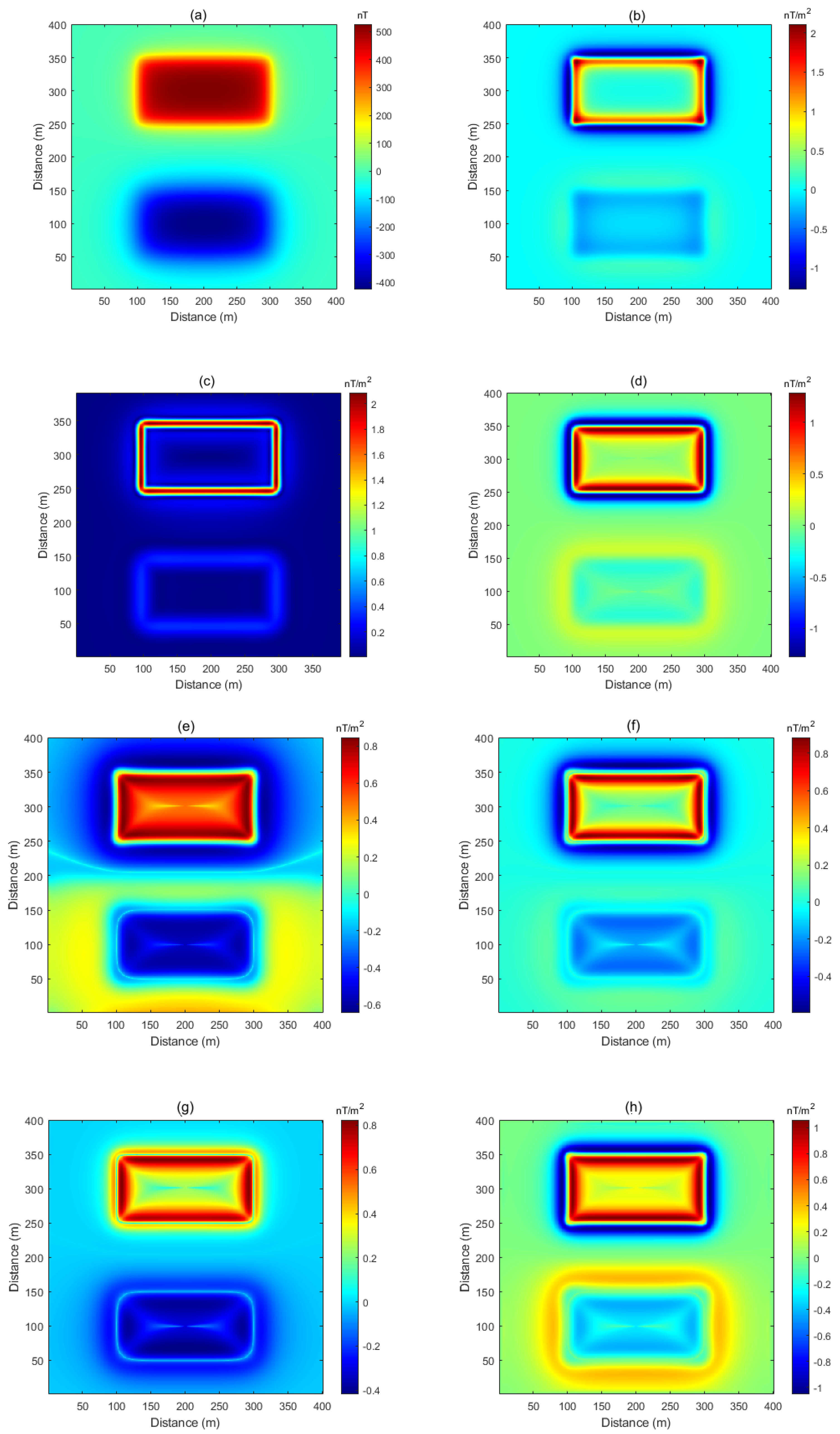
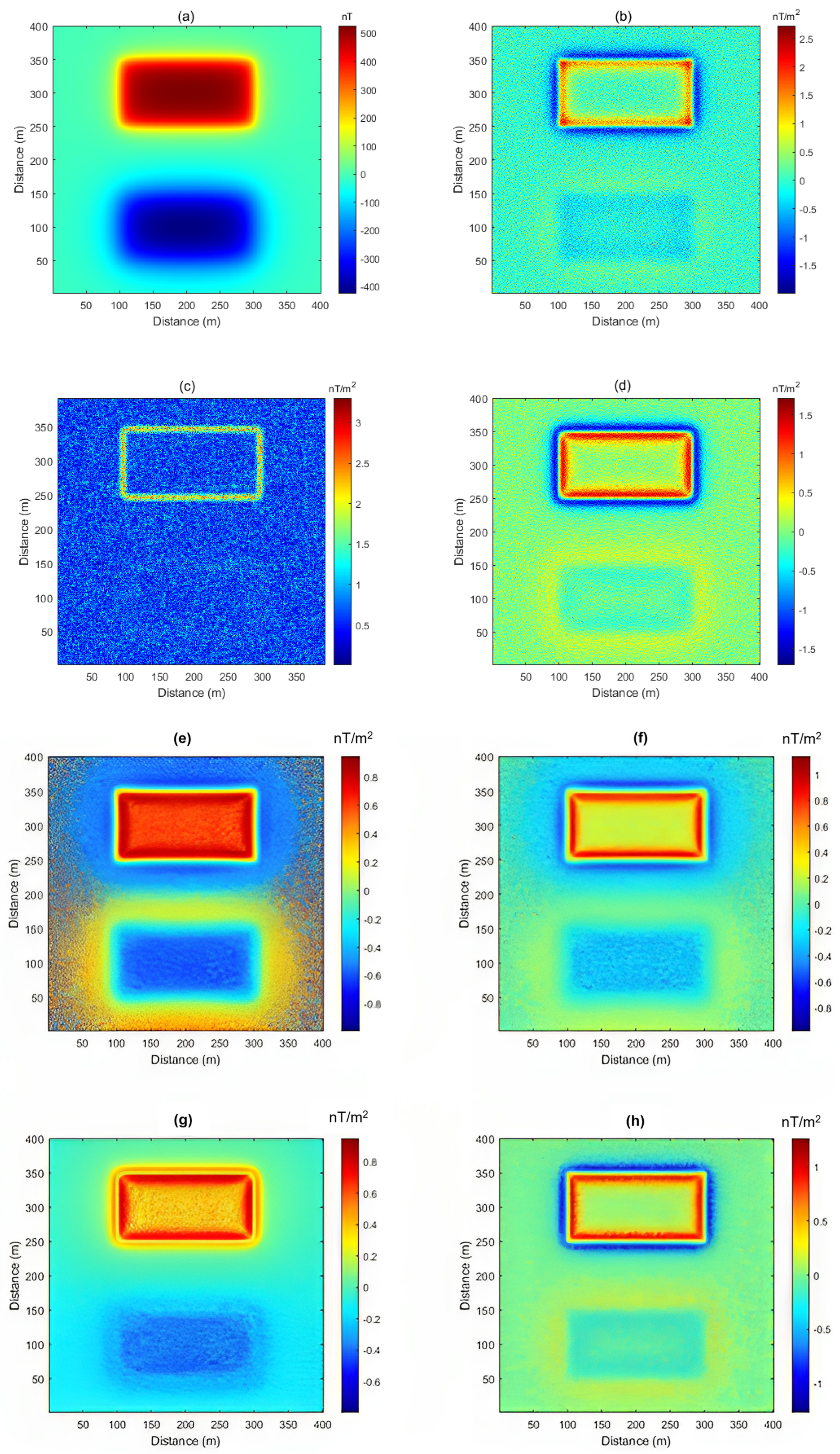
2. Materials and Methods

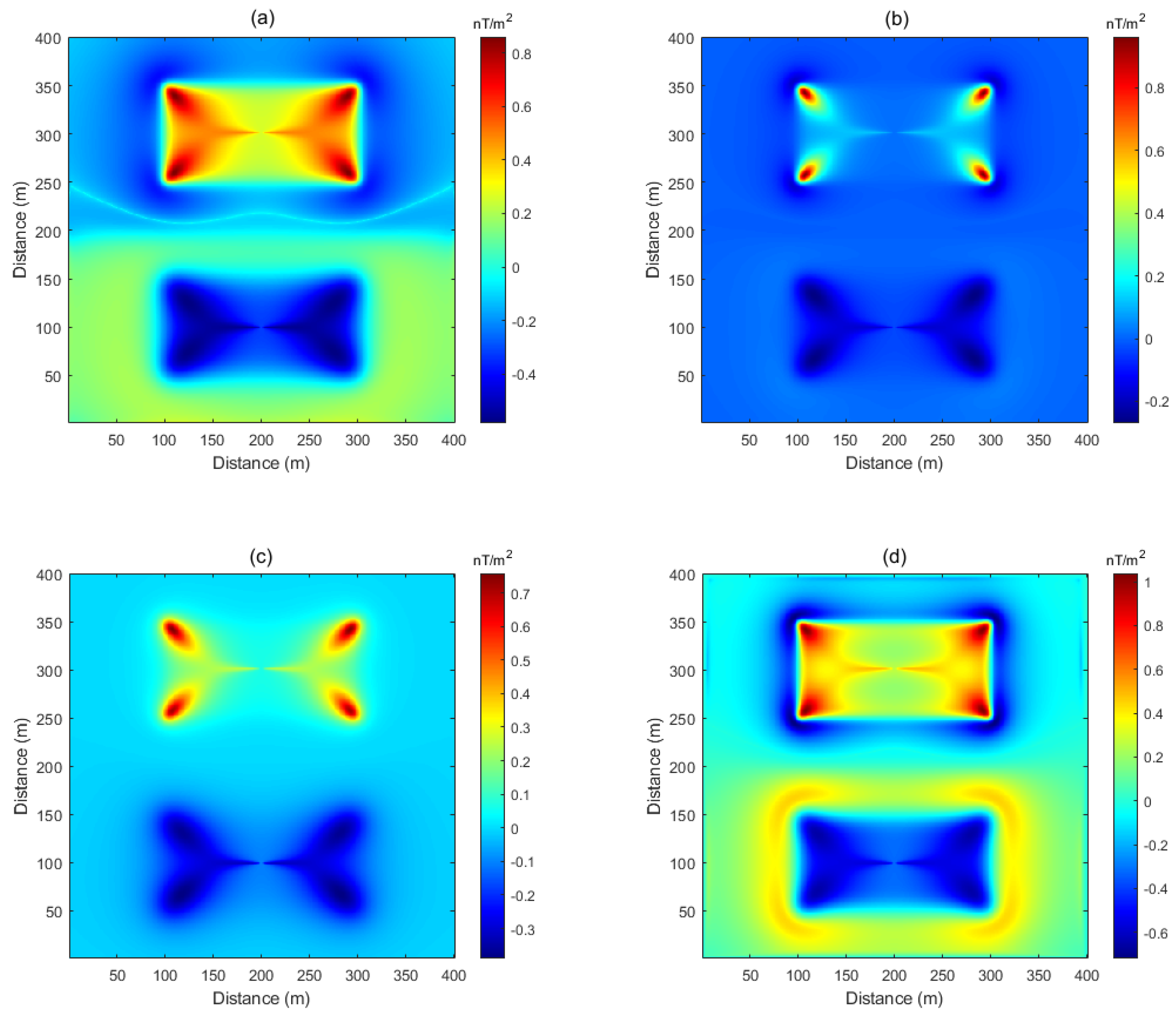
The uphill direction θ of a surface is given by the following [10].

$$\theta =\mathrm{t}\mathrm{a}{\mathrm{n}}^{-1}\left(\frac{\frac{df}{dy}}{\frac{df}{dx}}\right)$$

(6)

The first-order horizontal derivative in the uphill direction of a surface is just the TDX. The second-order horizontal derivative in the uphill direction is given by the following:

$$\frac{d^{2}f}{d{x}_{\theta }^2}=\frac{\frac{d^{2}f}{d{x}_{}^2}{\left(\frac{df}{dx}\right)}^2+2\frac{d^{2}f}{dxdy}\frac{df}{dx}\frac{df}{dy}+\frac{d^{2}f}{d{y}_{}^2}{\left(\frac{df}{dy}\right)}^2}{{\left(\frac{df}{dx}\right)}^2+{\left(\frac{df}{dy}\right)}^2}$$

(7)

which is closely related to the profile curvature of the data [6]. For two-dimensional structures, such as dykes and contacts, this reduces to d²f/dx² in the orthogonal direction to the structure. While the first-order horizontal derivative in the direction orthogonal to θ (i.e., along the contours of the data) is zero, the second-order horizontal derivative is given by the following:

$$\frac{d^{2}f}{d{x}_{\theta +\pi /2}^2}=\frac{\frac{d^{2}f}{d{x}_{}^2}{\left(\frac{df}{dy}\right)}^2-2\frac{d^{2}f}{dxdy}\frac{df}{dx}\frac{df}{dy}+\frac{d^{2}f}{d{y}_{}^2}{\left(\frac{df}{dx}\right)}^2}{{\left(\frac{df}{dx}\right)}^2+{\left(\frac{df}{dy}\right)}^2}$$

(8)

which is closely related to the plan curvature of the data [6]. For two-dimensional structures, such as dykes and contacts, this is zero in the orthogonal direction to the structure (because df/dy and d²f/dy² are zero). Equations (7) and (8) can be used to modify Equation (5) in the following manner:

$$F_{\theta }={\left|\frac{d^{2}f}{d{x}_{\theta }^2}\right|}^{\alpha }·\mathrm{s}\mathrm{i}\mathrm{n}\left(T_{\gamma }\right)$$

(9)

and

$$F_{\varphi }={\left|\frac{d^{2}f}{d{x}_{\theta +\pi /2}^2}\right|}^{\alpha }·\mathrm{s}\mathrm{i}\mathrm{n}\left(T_{\gamma }\right)$$

(10)

where Tγ is the tilt angle of order γ, i.e.,

$$T_{\gamma }=\mathrm{t}\mathrm{a}{\mathrm{n}}^{-1}\left(\frac{\frac{d^{\gamma }f}{d{z}^{\gamma }}}{\sqrt[2]{{\left(\frac{d}{dx}\left(\frac{d^{\gamma -1}f}{d{z}^{\gamma -1}}\right)\right)}^2+{\left(\frac{d}{dy}\left(\frac{d^{\gamma -1}f}{d{z}^{\gamma -1}}\right)\right)}^2}}\right)$$

(11)

For example, when γ = 1, T_γ just becomes the standard tilt angle (Equation (3)). Higher values of γ produce sharper images at the cost of greater sensitivity to noise.

3. Results

Figure 1 shows the application of F_θ to synthetic magnetic data from a simple block model. Because of the similarity of Equation (7) to the profile curvature, it is expected that the filter will enhance the edges of anomalies, and this is in fact the case. For comparison, the second vertical derivative of the data and the first vertical derivative of the TDX are also shown. As α → 0, then F_θ → sin(T_γ). Notably, 0.25 < α < 0.5 was found to be the most useful in practice, although these values are dataset dependant. Increasing the value of γ sharpens the result (see Figure 1g,h), though with the obvious caveat with respect to noise because of the use of higher order derivatives.

F_ϕ is complementary to F_θ in that it primarily enhances ridges/valleys and corners rather than edges, as is shown in Figure 2. Similarly to F_θ, as α → 0, then F_ϕ → sin(T_γ), and values of α between 0.25 and 0.5 were found to be the most useful in practice. Comparing Figure 2c,d shows that increasing γ does add some edge enhancement to the result, but again, noise will be an issue. Computationally, it only took 0.15 s to calculate F_θ and F_ϕ from a 450 × 450 point dataset on an Intel Core i7-5820K CPU (Intel Corp Company, Santa Clara, CA, USA) running at 3.30 GHz with 64 GB RAM, so the methods are not computationally intensive.

When random noise with an amplitude of 0.1% of that of the peak anomaly is added to the data, then all of the filters that were demonstrated in Figure 1 and Figure 2 have issues (see Figure 3), due to them all being second-order derivative-based. However, F_θ does not appear any worse in this regard than the second vertical derivative (Figure 3b), and actually seems less affected than the TDX of the first vertical derivative (Figure 3c). The noise sensitivity of F_ϕ is similar to that of F_θ.

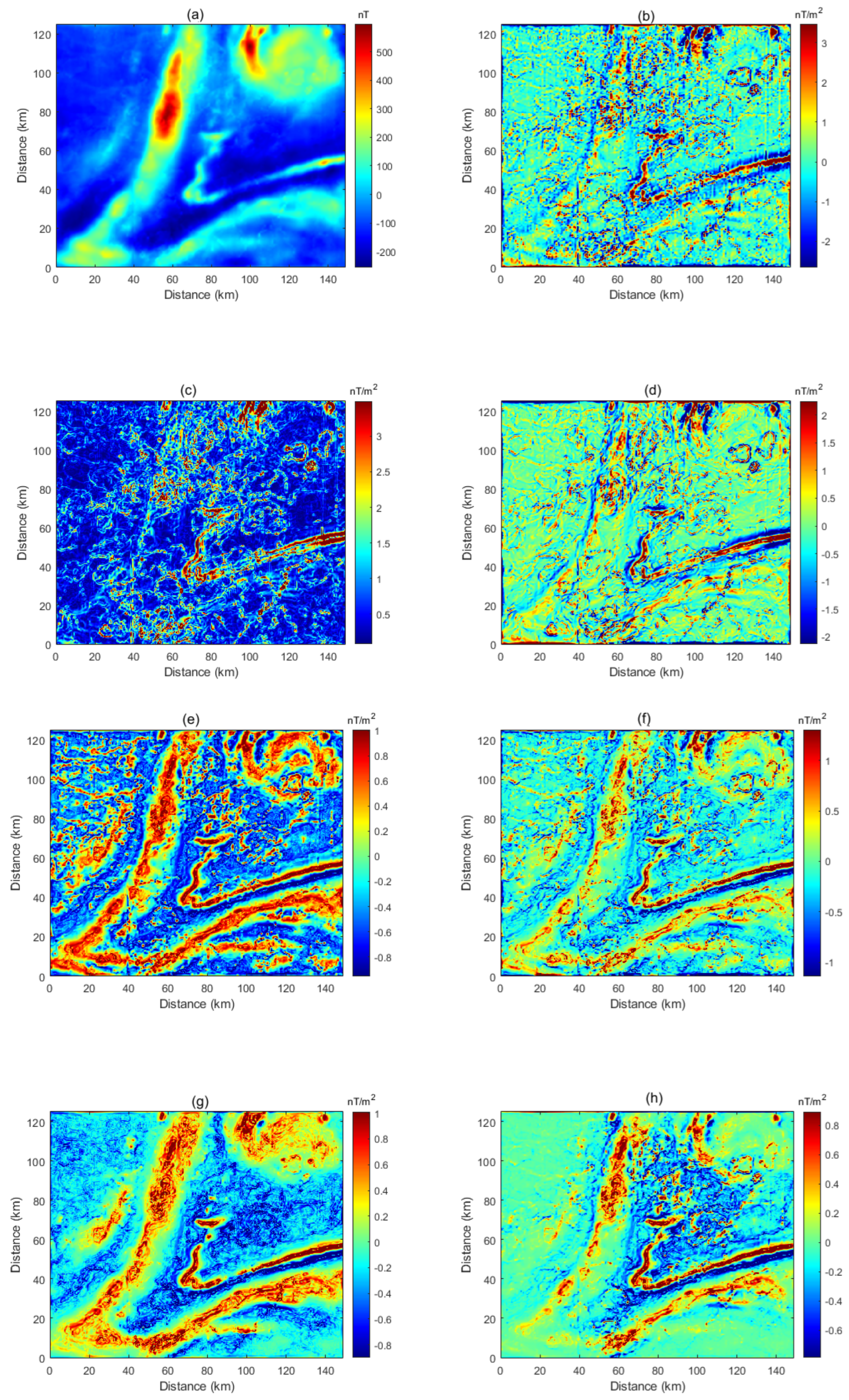
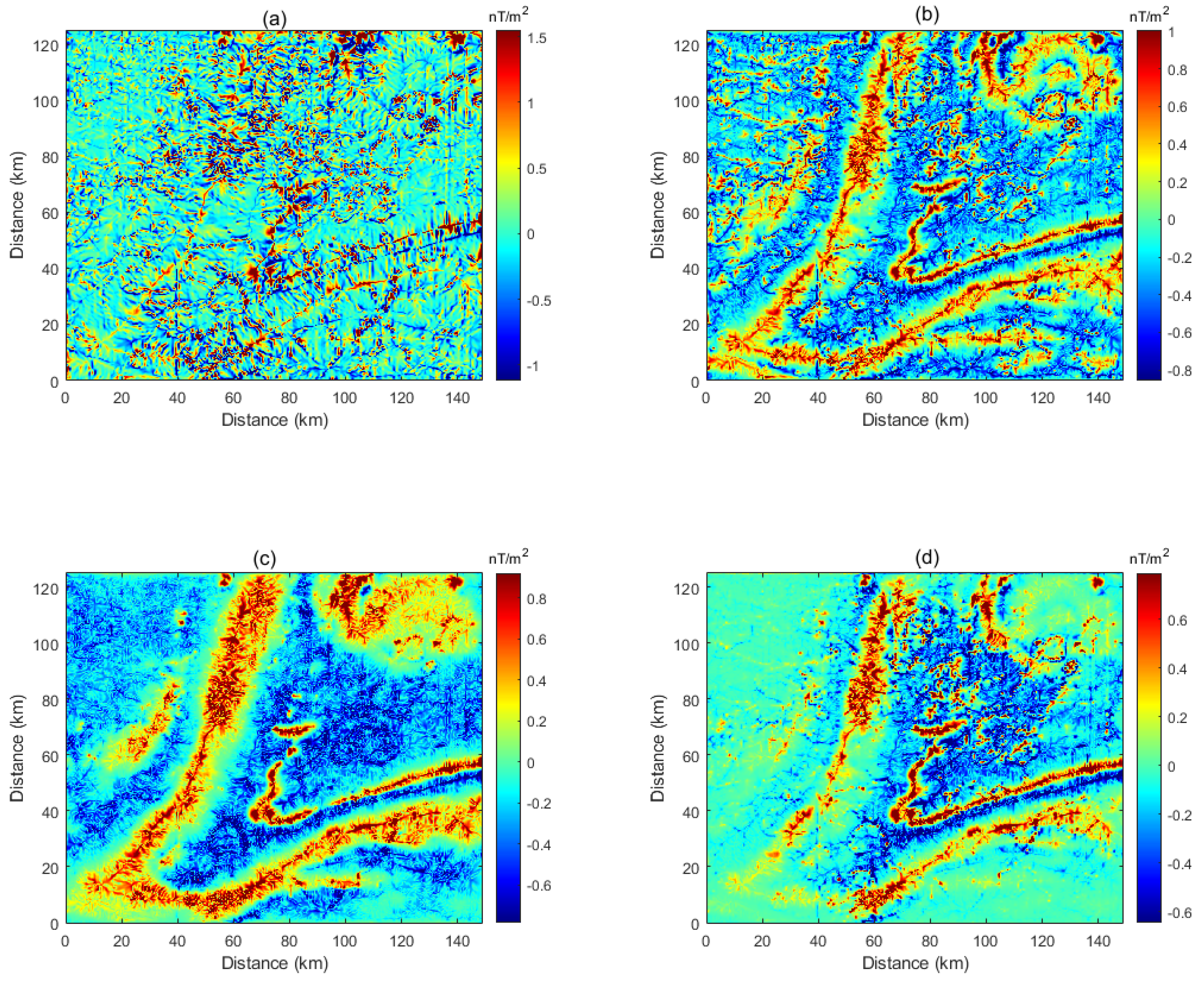
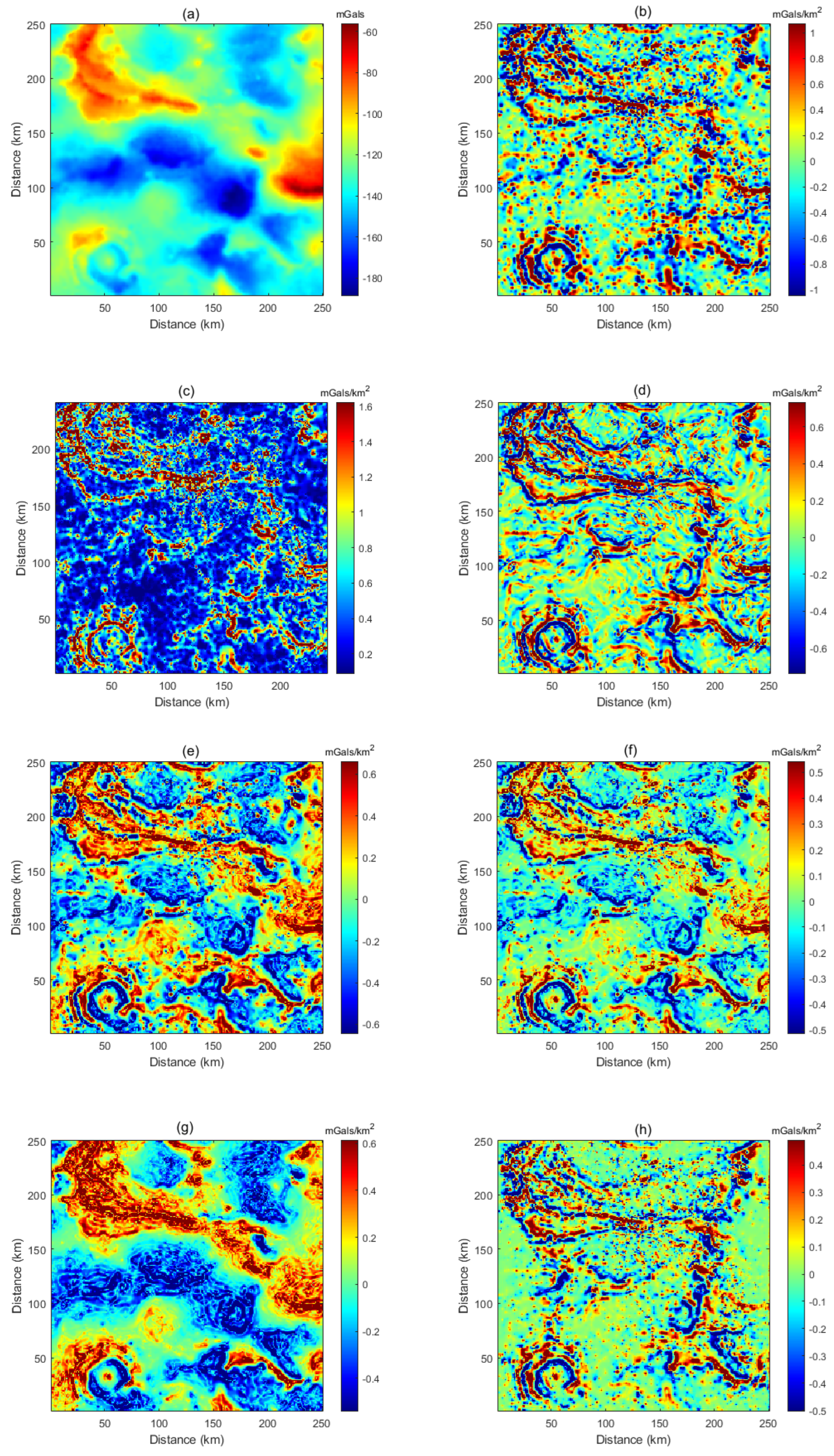
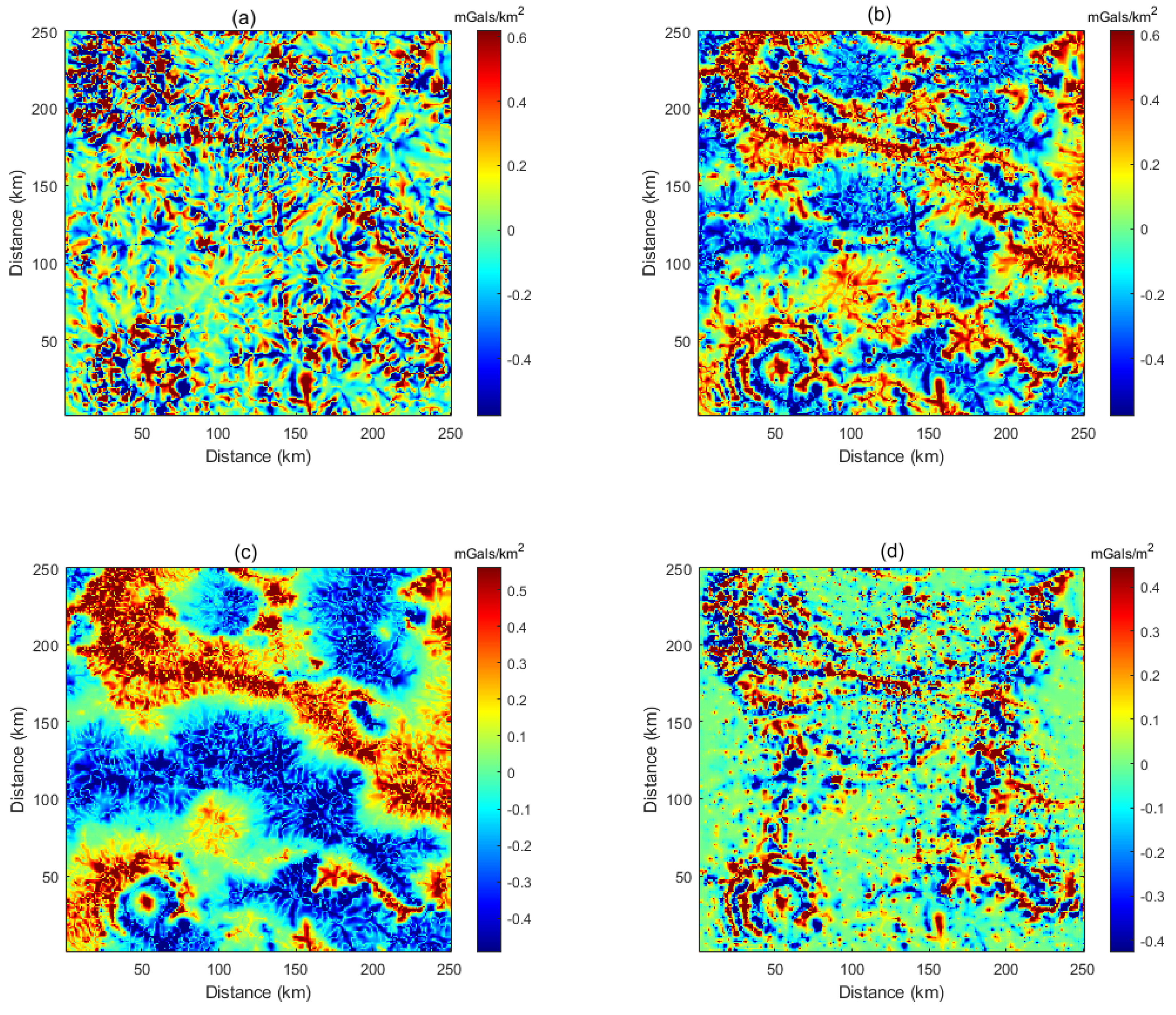
Application to Gravity and Magnetic Data from South Africa

Figure 4 shows gravity data from a portion of the Witwatersrand basin, South Africa (lower left). The basin is an important source of gold and has been mined for over 100 years [3]. The upper portion of the data shows part of the Bushveld igneous complex, which is also of great economic value, this time for platinum and related minerals [2]. The second vertical derivative image (Figure 4b) and the first vertical derivative of the TDX (Figure 4c) have brought out detail but are also noisy. Regarding the second horizontal derivative in the uphill direction (Equation (7)), Figure 4d appears to be slightly less noisy and shows greater continuity around the curved boundaries of the many geological features that are present in the image. F_θ (Figure 4e,f) significantly improves on Figure 4d. Different values of α and γ are used for comparison, with α = 0.5 and γ =1.0 arguably giving the best results in this case (Figure 4e). Regarding the second horizontal derivative in the contour direction (Equation (8)), Figure 5a has emphasised the ridges and valleys on the data, leading to radial patterns forming on the peaks of near circular features, such as the Vredefort dome impact structure in the lower left of the image [11]. F_ϕ, computed with different values of α and γ is also shown. All of the images possess greater continuity along the ridges/valleys than is present in Figure 5a.

Regional aeromagnetic data over a portion of the Trompsberg anomaly, South Africa, are shown in Figure 6a. The anomaly is thought to be associated with a sill and also possesses a significant gravity high [12]. The data is unfortunately of poor quality, and the NS flight lines (1 km spacing) are clearly visible in many of the images, such as the second vertical derivative (Figure 6b). The F_θ images again improve upon the previous images (Figure 6b–d) and are particularly effective in bringing out detail in the prominent fold structures that are visible in the area. Although the second horizontal derivative in the contour direction (Equation (8); Figure 7a) is badly affected by the noise and shows little detail of any value, F_ϕ is much more effective in tracking the ridges and valleys of the anomalies without being affected by the flight line effects.

4. Conclusions

Two new second-order derivative-based filters have been introduced that compared favourably to existing filters, such as the second vertical derivative, when they were applied to synthetic and real datasets. The filters do not appear to be any more sensitive to noise than do other comparable filters and were not computationally intensive to apply.

References

1. Cawthorn, R.G.; Cooper, G.R.J.; Webb, S.J. Connectivity between the Eastern and Western limbs of the Bushveld complex. S. Afr. J. Geol. 1998, 101, 291–298. [Google Scholar] [CrossRef]
2. Eales, H.V. A First Introduction to the Geology of the Bushveld Complex and Those Aspects of Geology That Relate to It; Council for Geoscience: Pretoria, South Africa, 2001; 84p. [Google Scholar]
3. Frimmel, H.E.; Groves, D.I.; Kirk, J.; Ruiz, J.; Chesley, J.; Minter, W.E.L. The formation and preservation of the Witwatersrand goldfields, the world’s largest gold province. Econ. Geol. 2005, 100, 1051–1052. [Google Scholar] [CrossRef]
4. Nabighian, M.N. Toward a three-dimensional automatic interpretation of potential field data via generalized Hilbert trans-forms: Fundamental relations. Geophysics 1984, 49, 957–966. [Google Scholar] [CrossRef]
5. Miller, H.G.; Singh, V. Potential field tilt—A new concept for location of potential field sources. J. Appl. Geophys. 1994, 32, 213–217. [Google Scholar] [CrossRef]
6. Roberts, A. Curvature attributes and their applications to 3D interpreted horizons. First Break 2001, 19, 85–100. [Google Scholar] [CrossRef]
7. Cooper, G.R.J. Processing Potential Field Data in the Amplitude/Phase Domain. Geophys. Prospect. 2019, 67, 455–464. [Google Scholar] [CrossRef]
8. Gonzalez, R.C.; Woods, R.E. Digital Image Processing, 3rd ed.; Prentice Hall: Upper Saddle River, NJ, USA, 2007; p. 187. [Google Scholar]
9. Cooper, G.R.J. Amplitude-Balanced Edge Detection Filters for Potential Field Data. Explor. Geophys. 2023, in press. [CrossRef]
10. Starck, J.L.; Murtagh, F. Astronomical Image and Data Analysis; Springer: Berlin, Germany, 2006; p. 18. ISBN 3-540-42885-2. [Google Scholar]
11. Gibson, R.L.; Reimold, W.U. The significance of the Vredefort Dome for the thermal and structural evolution of the Witwa-tersrand Basin, South Africa. Mineral. Petrol. 1999, 66, 5–23. [Google Scholar] [CrossRef]
12. Buchmann, J.P. Exploration of a geophysical anomaly at Trompsburg, Orange Free State, South Africa. Trans. Geol. Soc. S. Afr. 1960, 63, 1–10. [Google Scholar]
Figure 1. (a) Magnetic data from the two blocks whose outlines are shown. The field inclination/declination was −90°/0°, and the depths of the blocks were 10 km (upper) and 25 km (lower). The magnetisation of the blocks was ±1 A/m. (b) Second vertical derivative of the data shown in (a). (c) TDX of the first vertical derivative of the data. (d) Second derivative in the uphill direction of the data (Equation (7)). (e) Fθ with α = 0.25 and γ = 1 (Equation (9)). (f) Fθ with α = 0.75 and γ = 1. (g) Fθ with α = 0.25 and γ = 0. (h) Fθ with α = 0.25 and γ = 2.
Minerals 13 01229 g001
Figure 2. (a) Second derivative in the contour direction (Equation (8) of the data shown in Figure 1a). (b) Fϕ with α = 0.5 and γ = 1. (c) Fϕ with α = 0.5 and γ = 0.25. (d) Fϕ with α = 0.5 and γ = 1.75.
Minerals 13 01229 g002
Figure 3. (a) Magnetic data from the two blocks whose outlines are shown. The field inclination/declination was −90°/0°, and the depths of the blocks were 10 km (upper) and 25 km (lower). The magnetisation of the blocks was ±1 A/m. Uniformly distributed random noise with an amplitude of 0.1% of the maximum data amplitude was added to the data. (b) Second vertical derivative of the data shown in (a). (c) TDX of the first vertical derivative of the data. (d) Second derivative in the uphill direction of the data (Equation (7)). (e) Fθ with α = 0.25 and γ = 1 (Equation (9)). (f) Fθ with α = 0.75 and γ = 1. (g) Fθ with α = 0.25 and γ = 0. (h) Fθ with α = 0.25 and γ = 2.
Minerals 13 01229 g003
Figure 4. (a) Gravity data from a portion of the Witwatersrand basin, South Africa. The grid interval is 1.0 km. (b) Second vertical derivative of the data shown in (a). (c) TDX of the first vertical derivative of the data. (d) Second derivative in the uphill direction of the data (Equation (7)). (e) Fθ with α = 0.5 and γ = 1 (Equation (9)). (f) Fθ with α = 0.95 and γ = 1. (g) Fθ with α = 0.25 and γ = 0. (h) Fθ with α = 0.25 and γ = 2.
Minerals 13 01229 g004
Figure 5. (a) Second derivative in the contour direction (Equation (8)) of the data shown in Figure 4a. (b) Fϕ with α = 0.5 and γ = 1. (c) Fϕ with α = 0.5 and γ = 0.25. (d) Fϕ with α = 0.5 and γ = 1.5.
Minerals 13 01229 g005
Figure 6. (a) Pole-reduced magnetic data from South Africa, upward continued by 400 m. The grid interval is 200 m. (b) Second vertical derivative of the data shown in (a). (c) TDX of the first vertical derivative of the data. (d) Second derivative in the uphill direction of the data (Equation (7)). (e) Fθ with α = 0.25 and γ = 1 (Equation (9)). (f) Fθ with α = 0.75 and γ = 1. (g) Fθ with α = 0.5 and γ = 0.25. (h) Fθ with α = 0.5 and γ = 0.95.
Minerals 13 01229 g006
Figure 7. (a) Second derivative in the contour direction (Equation (8) of the data shown in Figure 6a). (b) Fϕ with α = 0.5 and γ = 1. (c) Fϕ with α = 0.5 and γ = 0.25. (d) Fϕ with α = 0.5 and γ = 0.95.
Minerals 13 01229 g007
Disclaimer/Publisher’s Note: The statements, opinions and data contained in all publications are solely those of the individual author(s) and contributor(s) and not of MDPI and/or the editor(s). MDPI and/or the editor(s) disclaim responsibility for any injury to people or property resulting from any ideas, methods, instructions or products referred to in the content.