

In-Situ Study Methods Used in the Discovery of Sites of Modern Hydrothermal Ore Formation on the Mid-Atlantic Ridge

Abstract
1. Introduction
2. Materials and Methods
2.1. Sounding of the Water Column
2.2. Sounding by a Methane Sensor
2.3. Profiling by Towed Instrument Package
2.4. TV-Profiling
2.5. Hydroacoustic Underwater Positioning
3. Results and Discussion
3.1. Profiling by RIFT and MAK-1M
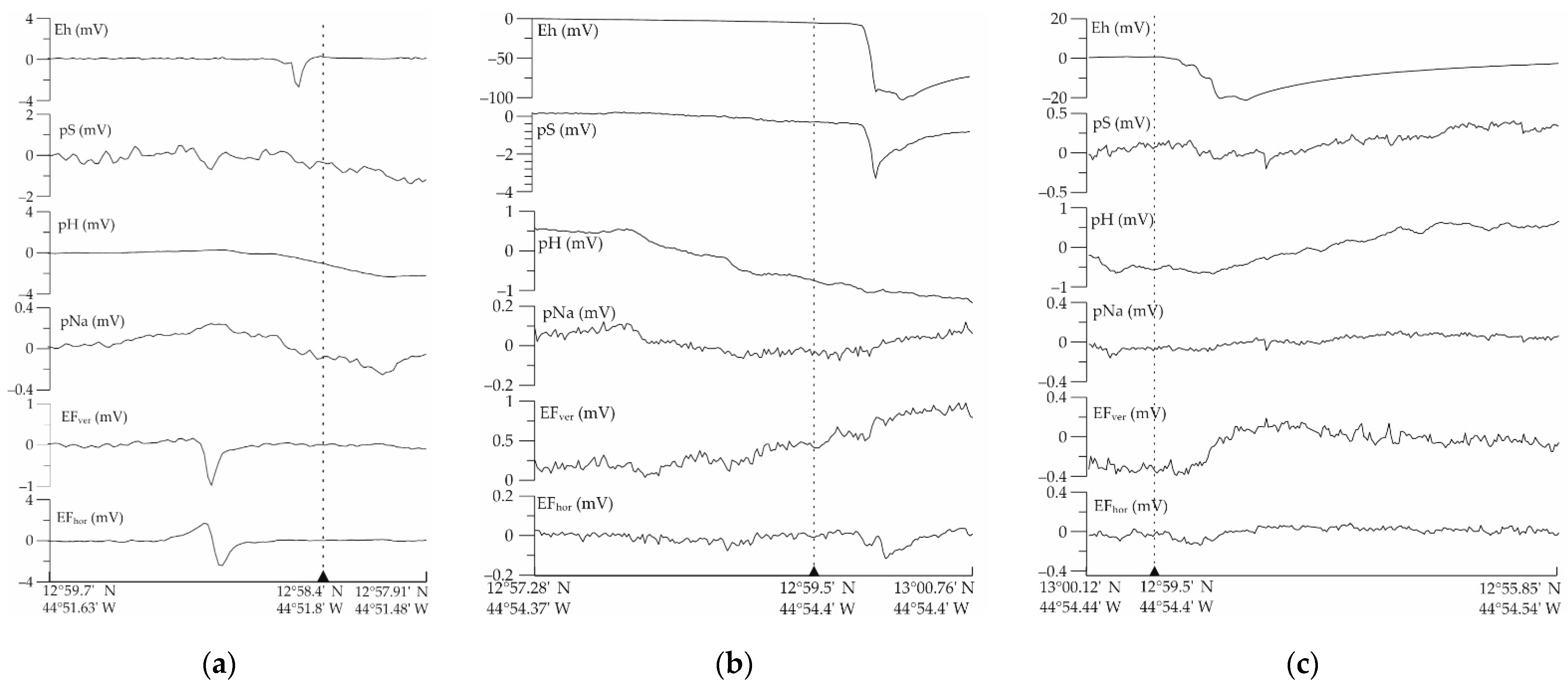
3.1.1. Ashadze Hydrothermal Cluster
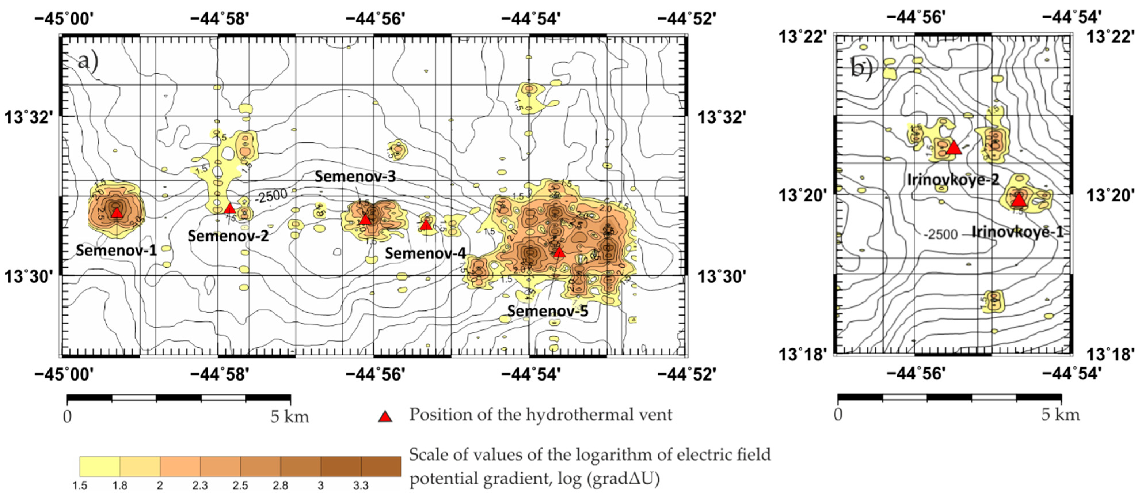
3.1.2. Peterburgskoye, Semenov and Irinovskoye Hydrothermal Areas
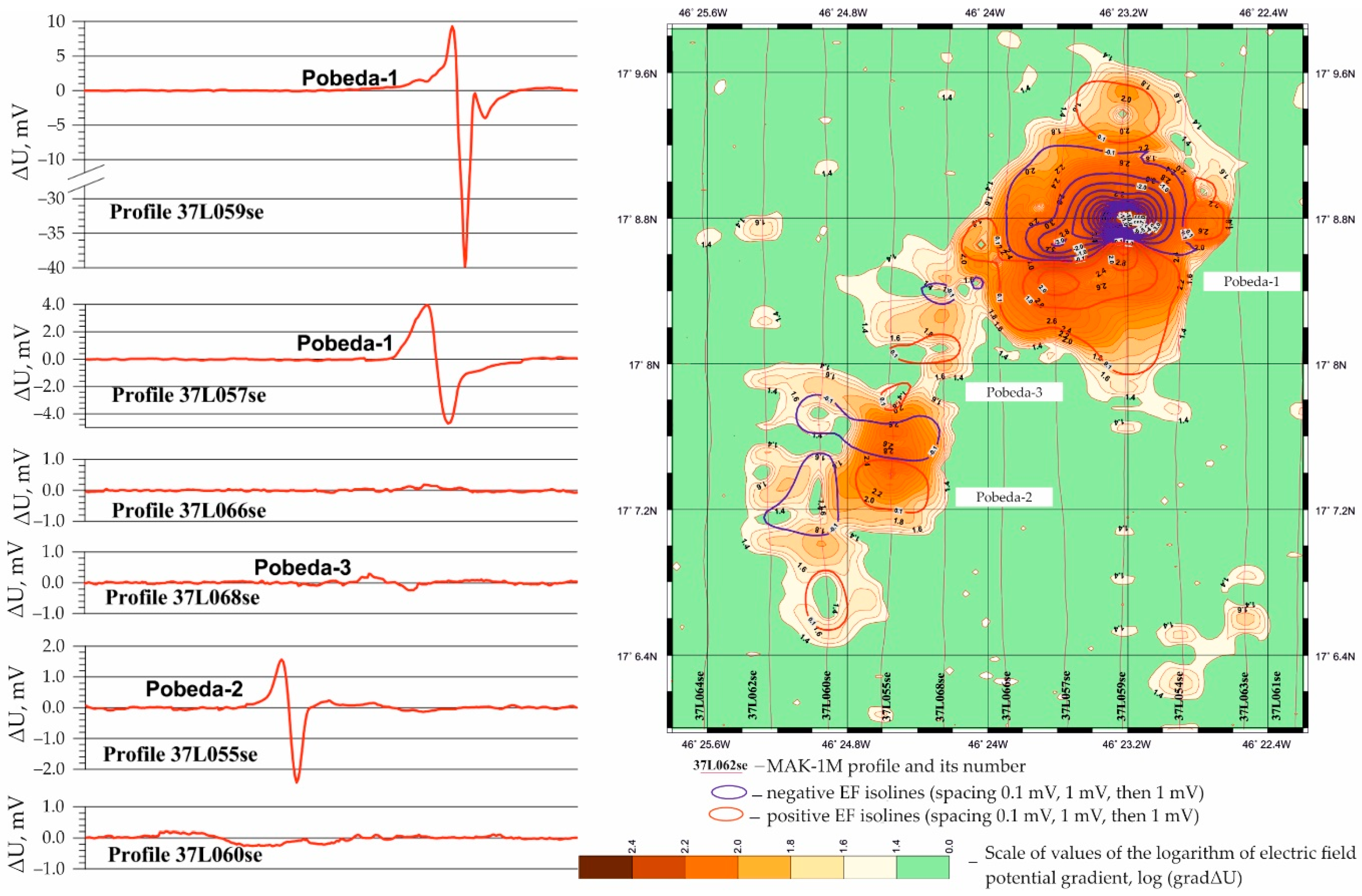
3.1.3. Pobeda Hydrothermal Cluster
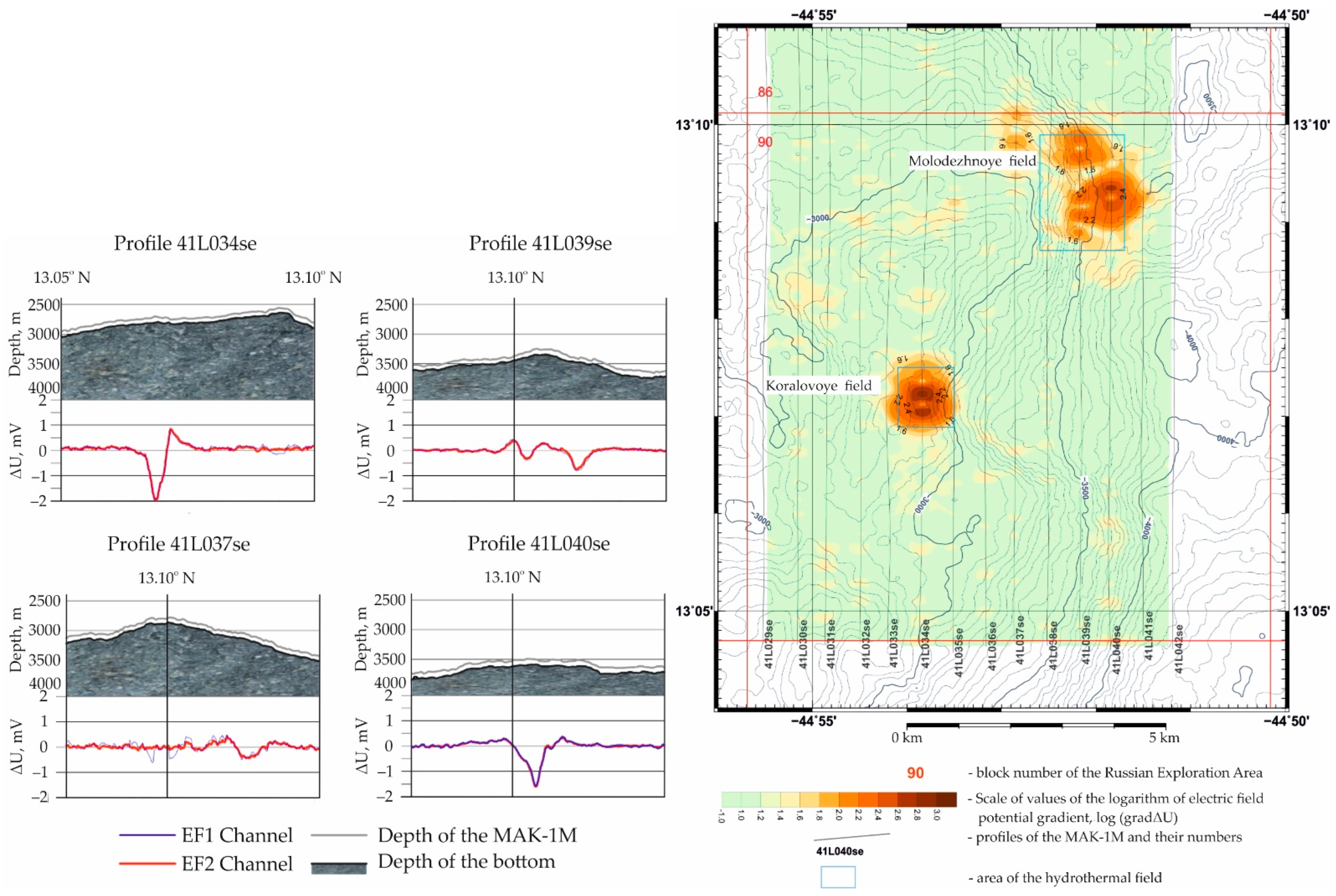
3.1.4. Molodezhnoye and Koralovoye HF’s
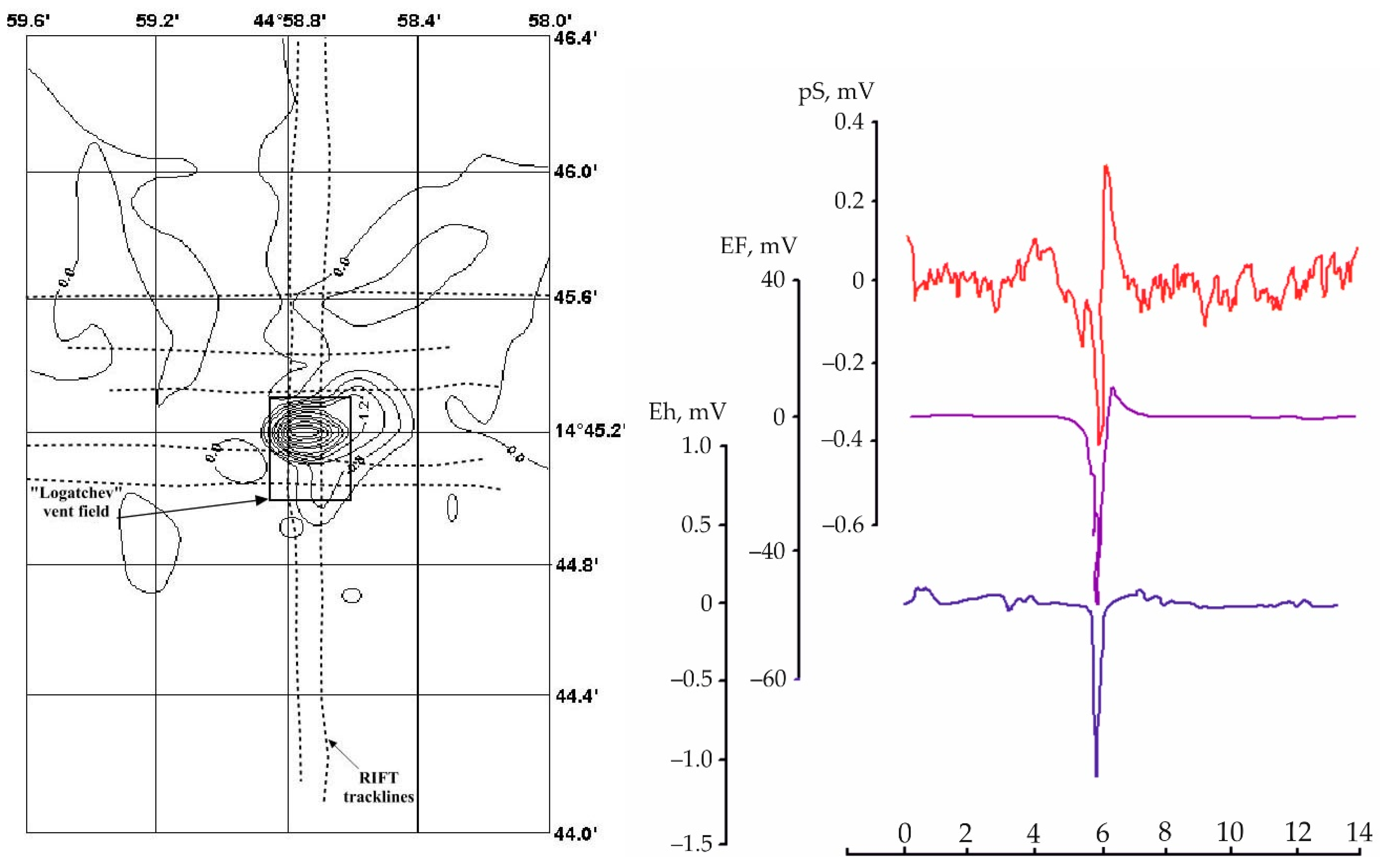
3.1.5. Logachev Hydrothermal Cluster
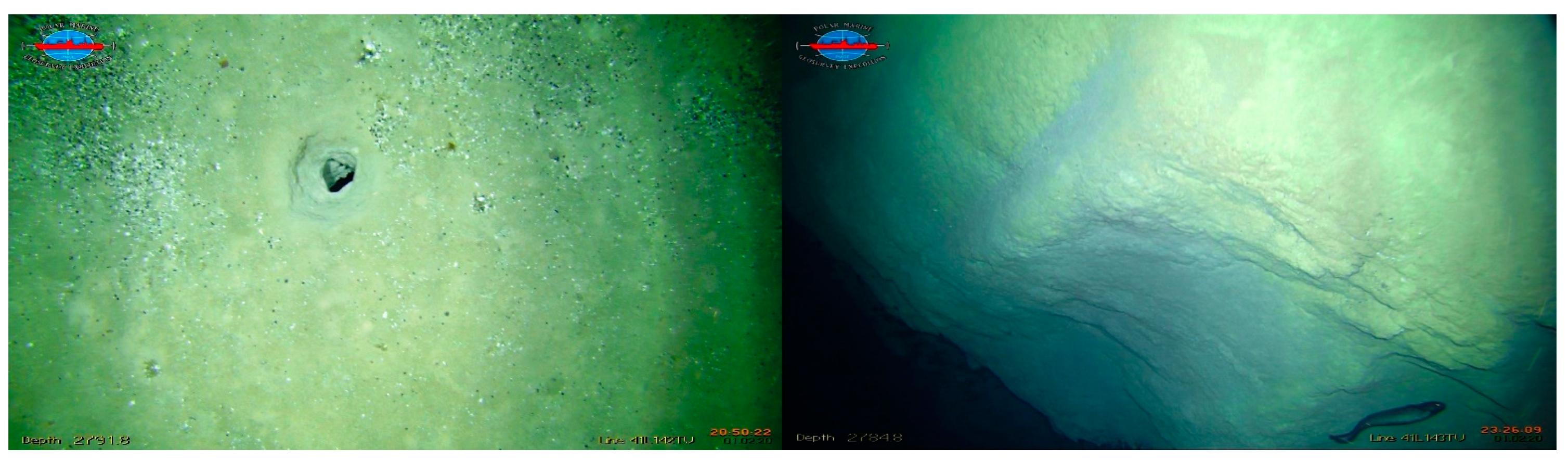
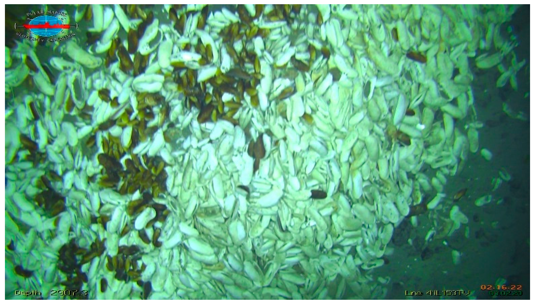
3.2. TV-Profiling
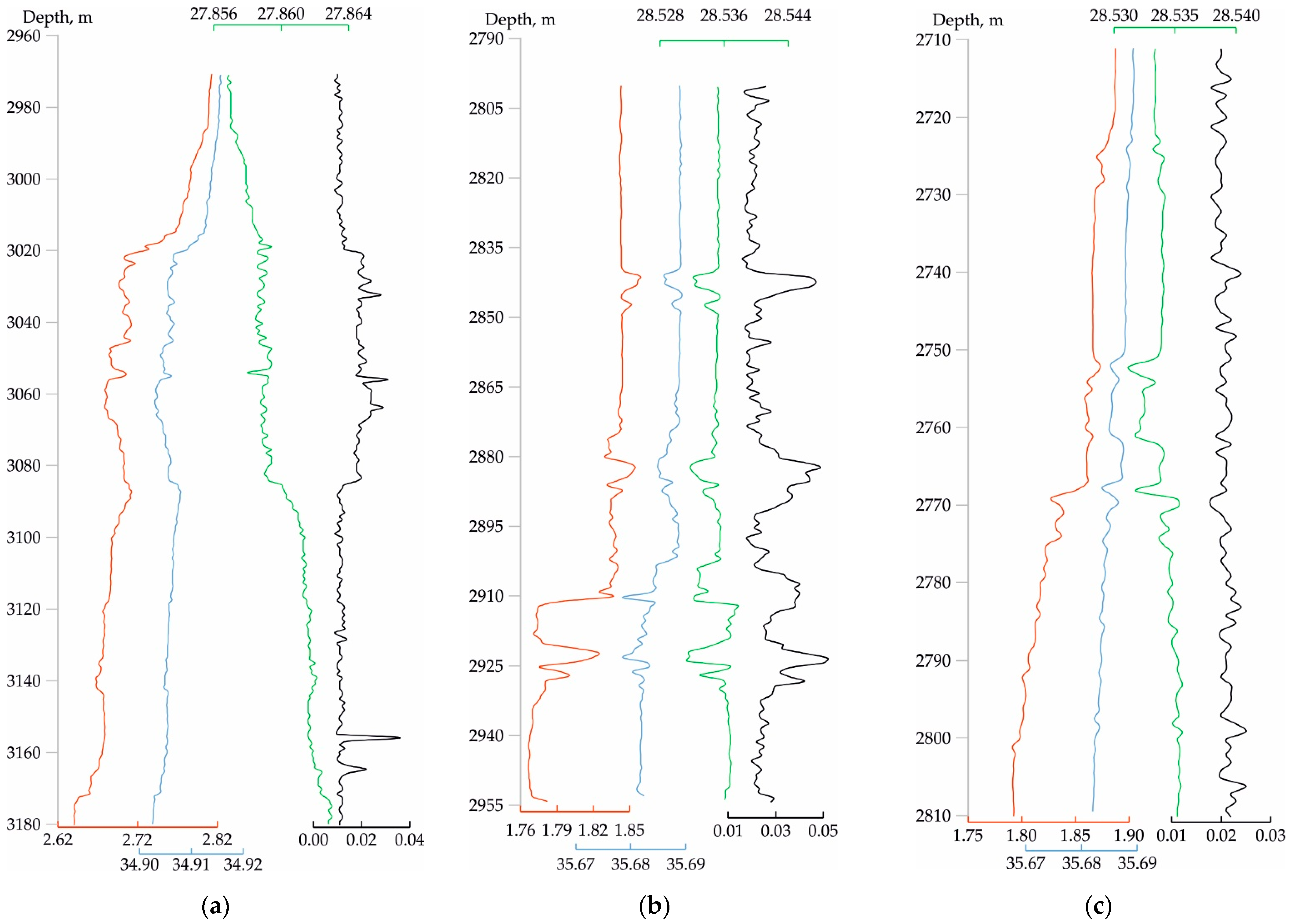
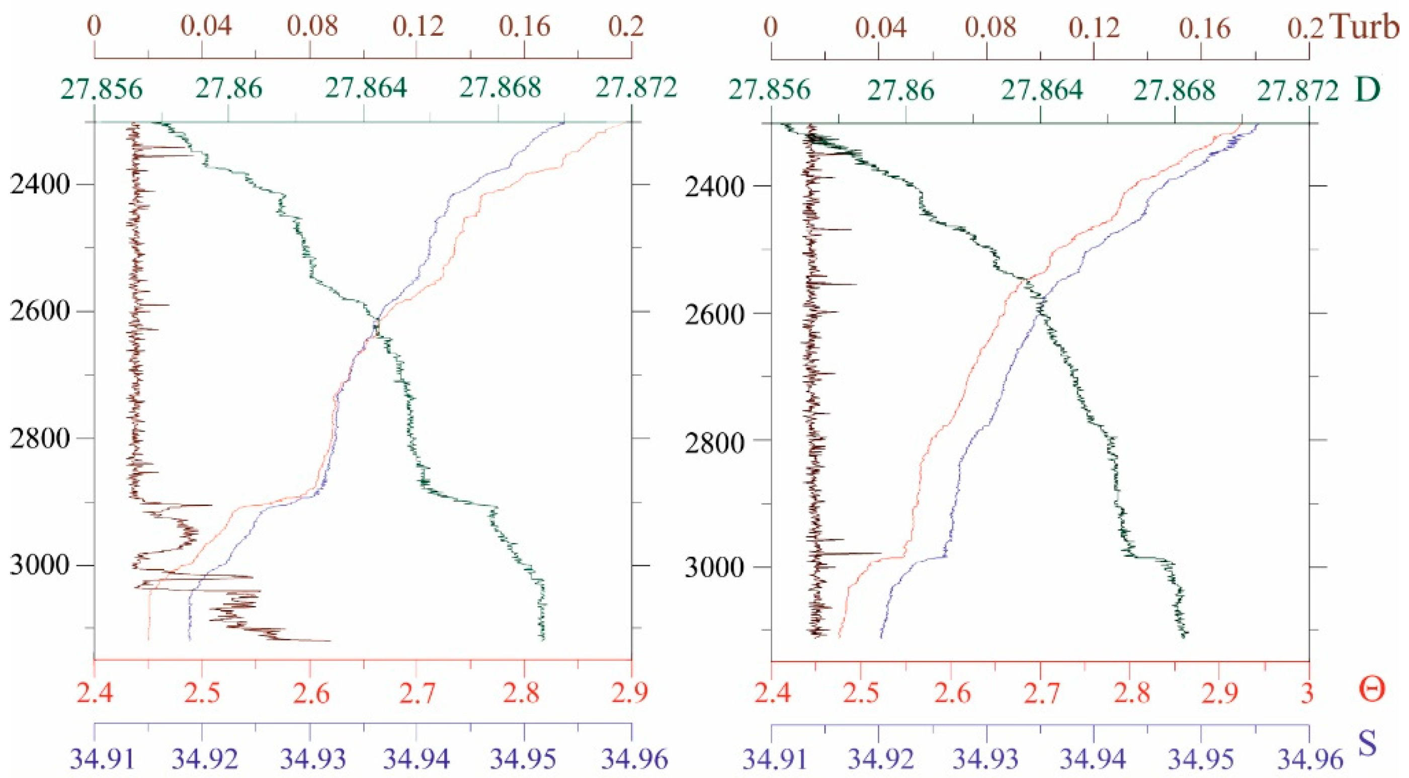
3.3. CTD-Sounding
3.4. Measurements using a Methane Sensor
3.4.1. Logachev Hydrothermal Cluster
3.4.2. Molodezhnoye and Koralovoye HF’s
4. Conclusions
- (1)
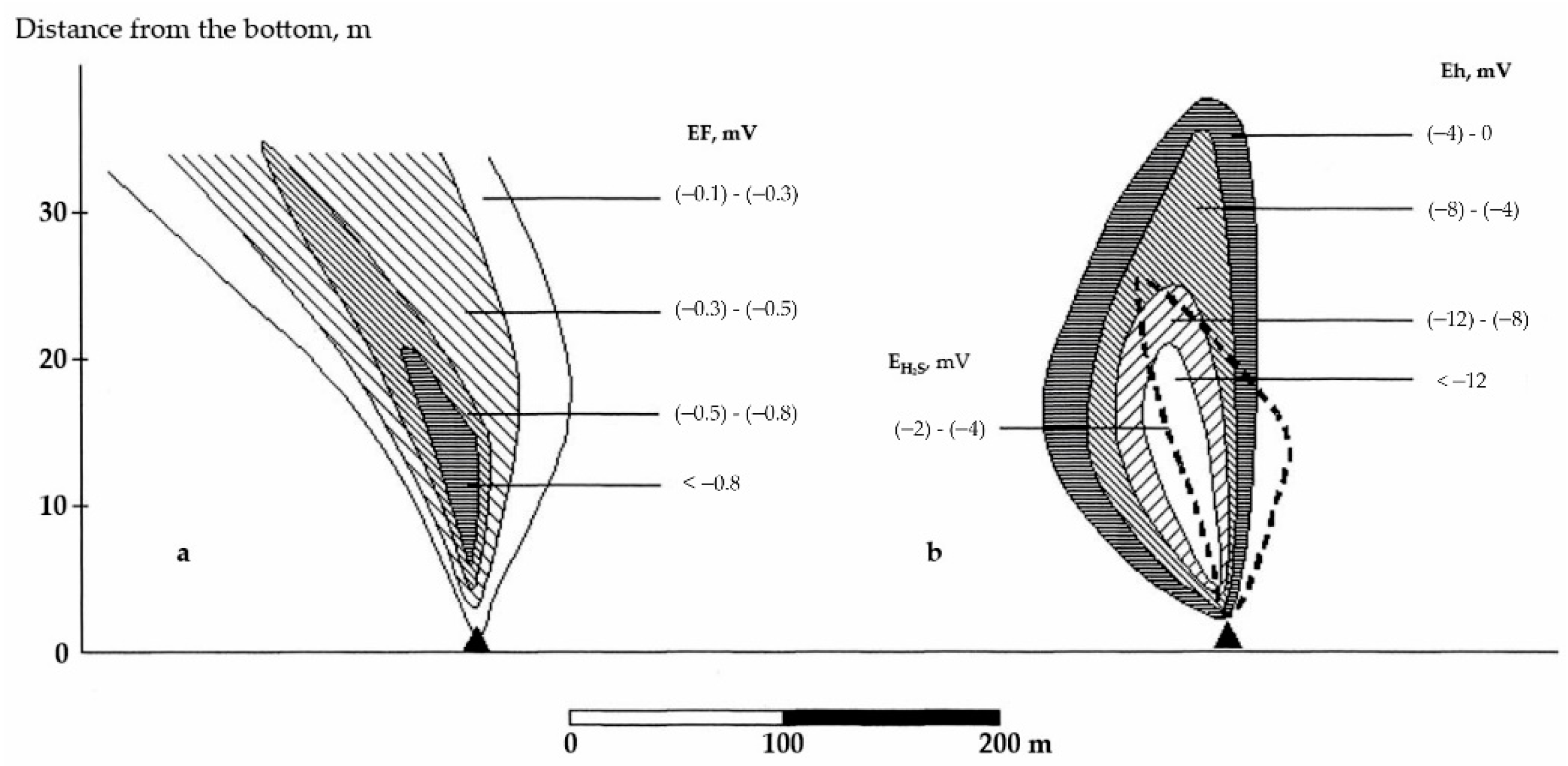
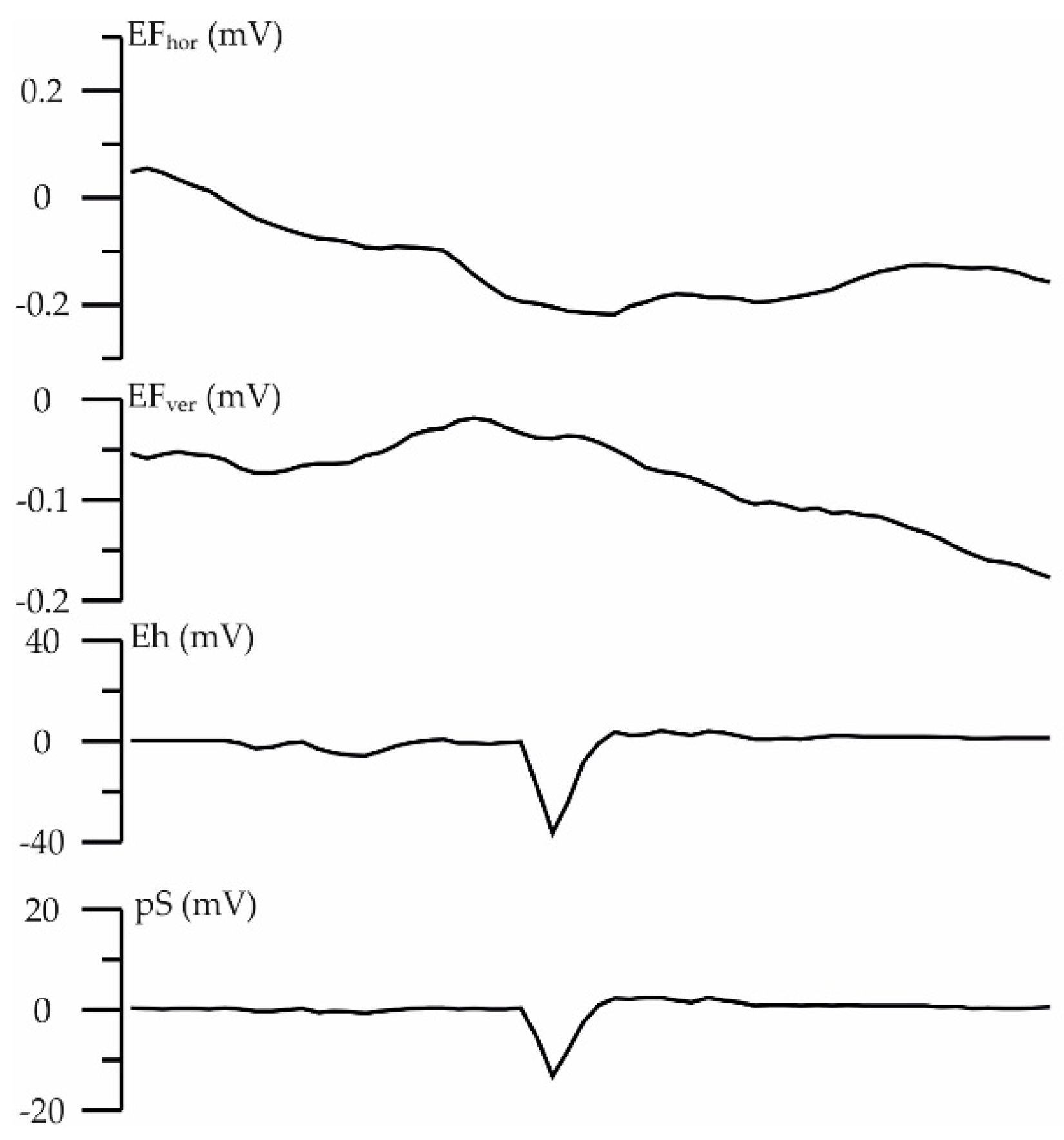
- Profiling by towed vehicles makes it possible to record geophysical (EF) and geochemical anomalies (Eh, pS, etc.). Geophysical anomalies are more often revealed near the bottom, while geochemical anomalies are expressed at 150–200 m from the bottom. Profiling should be conducted in two stages: in the ′′high′′ interval to determine geochemical anomalies and in the “low” interval to identify geophysical anomalies. The EF anomalies in the “low” and ′′high′′ intervals have different forms, apparently caused by different reasons—the polarization of the ores and the influence of metal sulfides in the plume, respectively. Geophysical and geochemical anomalies can be separated from each other at distances up to 1000 m, which may be due to the evolution of the plume. EF anomalies are a good search sign of high- and low-temperature discharge and even inactive fields.
- (2)
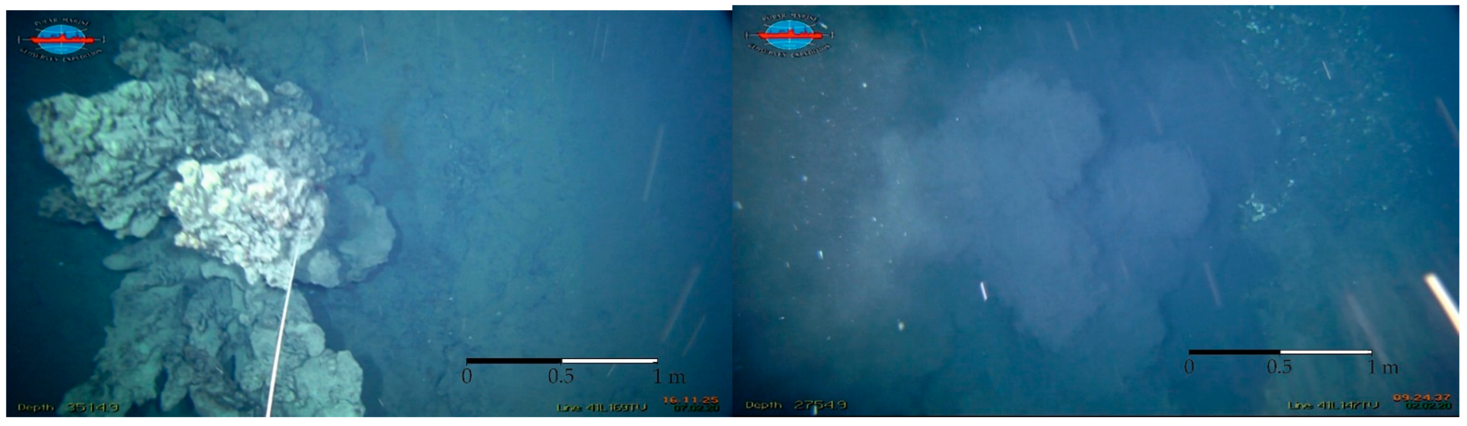
- TV profiling allows the detection of direct evidence of high–temperature discharge-hydrothermal structures and smokers’ black “smoke”. Lithification of sediments and accumulation of endemic hydrothermal fauna (e.g., mollusks Caliptogena sp.), which can be observed during teleprofiling, may be indirect signs of low-temperature discharge.
- (3)
- Based on the capacity, amplitude, position and sign of anomalies (turbidity, temperature, salinity and density), we have identified 6 types of complex geophysical anomalies. Types reflect the stage of plume formation, mineralization of end-members of hydrothermal fluid and the cause of its origin (anthropogenic or natural). CTD-sounding is a good method for detecting and verifying hydrothermal anomalies. However, this method cannot detect low-temperature discharging with due accuracy.
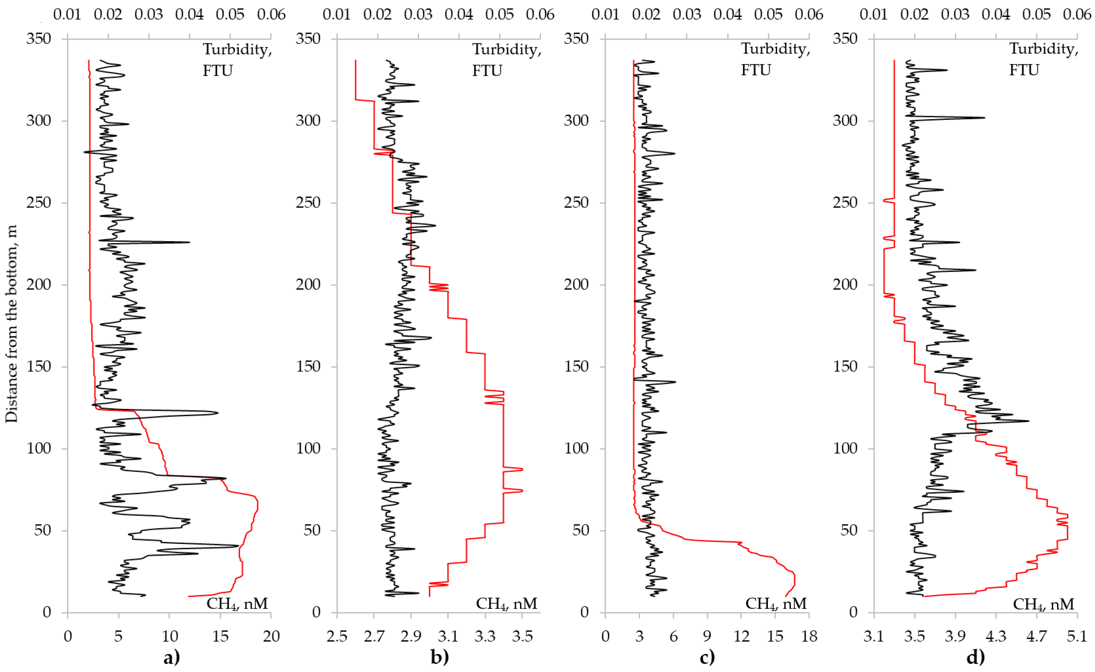
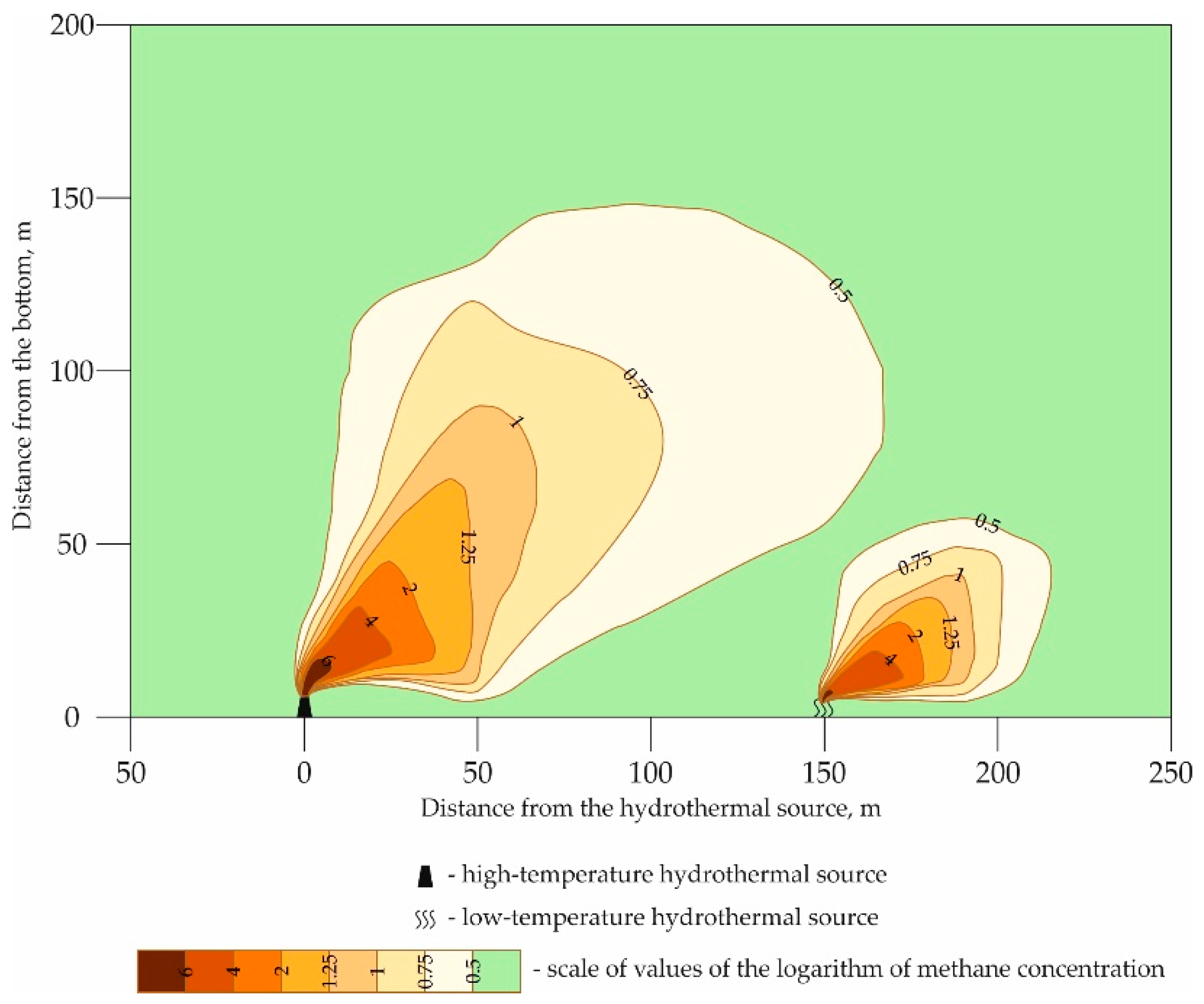
- (4)
- The methane sounding near the Logachev, Koralovoye, Molodezhnoye HF’s and the analysis of published data on CH4 concentrations in hydrothermal plumes revealed high variability in the behavior of this element. The maximum values of turbidity and methane can be 50–100 m apart from each other, and the height of the rise of CH4 above the bottom often does not exceed 200–300 m. Elevated concentrations of CH4 with the absence of distinct geophysical anomalies may indicate low-temperature discharging. The range of CH4 anomalies depends on several factors and can vary from the first 100 s of meters to the first 10 s of kilometers, thereby complicating the use of a methane sensor in search operations. A dense grid of profiles will allow high- and low-temperature sources to be detected with high accuracy.
Author Contributions
Funding
Data Availability Statement
Acknowledgments
Conflicts of Interest
References
- Zhang, Z.; Fan, W.; Bao, W.; Chen, C.T.A.; Liu, S.; Cai, Y. Recent developments of exploration and detection of shallow-water hydrothermal systems. Sustainability 2020, 12, 9109. [Google Scholar] [CrossRef]
- Corliss, J.B.; Dymond, J.; Gordon, L.I.; Edmond, J.M.; von Herzen, R.P.; Ballard, R.D.; Green, K.; Williams, D.; Bainbridge, A.; Crane, K.; et al. Submarine thermal spring on the Galapagos Rift. Science 1979, 203, 1073–1083. [Google Scholar] [CrossRef]
- Amon, D.J.; Gollner, S.; Morato, T.; Smith, C.R.; Chen, C.; Christiansen, S.; Currie, B.; Drazen, J.C.; Fukushima, T.; Gianni, M.; et al. Assessment of scientific gaps related to the effective environmental management of deep-seabed mining. Mar. Policy 2022, 138, 105006. [Google Scholar] [CrossRef]
- Hannington, M.; Jamieson, J.; Monecke, T.; Petersen, S.; Beaulieu, S. The abundance of seafloor massive sulfide deposits. Geology 2011, 39, 1155–1158. [Google Scholar] [CrossRef]
- Singer, D.A. Base and precious metal resources in seafloor massive sulfide deposits. Ore Geol. Rev. 2014, 59, 66–72. [Google Scholar] [CrossRef]
- Miller, K.A.; Thompson, K.F.; Johnston, P.; Santillo, D. An overview of seabed mining including the current state of development, environmental impacts, and knowledge gaps. Front. Mar. Sci. 2018, 4, 418. [Google Scholar] [CrossRef]
- Van Dover, C.L.; Arnaud-Haond, S.; Gianni, M.; Helmreich, S.; Huber, J.A.; Jaeckel, A.L.; Metaxas, A.; Pendleton, L.H.; Petersen, S.; Ramirez-Llodra, E.; et al. Scientific rationale and international obligations for protection of active hydrothermal vent ecosystems from deep-sea mining. Mar. Policy 2018, 90, 20–28. [Google Scholar] [CrossRef]
- Douville, E.; Charlou, J.L.; Oelkers, E.H.; Bienvenu, P.; Colon, C.J.; Donval, J.P.; Fouquet, Y.; Prieur, D.; Appriou, P. The rainbow vent fluids (36 14′ N, MAR): The influence of ultramafic rocks and phase separation on trace metal content in Mid-Atlantic Ridge hydrothermal fluids. Chem. Geol. 2002, 184, 37–48. [Google Scholar] [CrossRef]
- Costa, K.M.; Anderson, R.F.; McManus, J.F.; Winckler, G.; Middleton, J.L.; Langmuir, C.H. Trace element (Mn, Zn, Ni, V) and authigenic uranium (aU) geochemistry reveal sedimentary redox history on the Juan de Fuca Ridge, North Pacific Ocean. Geochim. Cosmochim. Acta 2018, 236, 79–98. [Google Scholar] [CrossRef]
- Mason, J.C.; Branch, A.; Xu, G.; Jakuba, M.V.; German, C.R.; Chien, S.; Bowen, A.D.; Hand, K.P.; Seewald, J.S. Evaluation of AUV Search Strategies for the Localization of Hydrothermal Venting. In Proceedings of the 30th International Conference on Automated Planning and Scheduling (ICAPS 2020), Nancy, France, 26–30 October 2020. [Google Scholar]
- Rumynin, V.G.; Nikulenkov, A.M.; Rozov, K.B.; Rozov, K.B.; Erzova, V.A. The status and trends in radioactive contamination of groundwater at a LLW-ILW storage facility site near Sosnovy Bor (Leningrad region, Russia). J. Environ. Radioact. 2021, 237, 106707. [Google Scholar] [CrossRef]
- Fang, Z.; Wang, W.X. Size speciation of dissolved trace metals in hydrothermal plumes on the Southwest Indian Ridge. Sci. Total Environ. 2021, 771, 145367. [Google Scholar] [CrossRef] [PubMed]
- Fouquet, Y.; Cambon, P.; Etoubleau, J.; Charlou, J.L.; OndréAs, H.; Barriga, F.J.; Cherkashov, G.; Semkova, T.; Poroshina, I.; Bohn, M. Geodiversity of Hydrothermal Processes along the Mid-Atlantic Ridge and Ultramafic-Hosted Mineralization: A New Type of Oceanic Cu-Zn-Co-Au Volcanogenic Massive Sulfide Deposit. In Diversity of Hydrothermal Systems on Slow Spreading Ocean Ridges; American Geophysical Union: Washington, DC, USA, 2013; Volume 188, pp. 321–367. [Google Scholar]
- Liao, S.; Tao, C.; Dias, Á.A.; Su, X.; Yang, Z.; Ni, J.; Liang, J.; Yang, W.; Liu, J.; Li, W.; et al. Surface sediment composition and distribution of hydrothermal derived elements at the Duanqiao-1 hydrothermal field, Southwest Indian Ridge. Mar. Geol. 2019, 416, 105975. [Google Scholar] [CrossRef]
- Lough, A.J.M.; Homoky, W.B.; Connelly, D.P.; Comer-Warner, S.A.; Nakamura, K.; Abyaneh, M.K.; Kaulich, B.; Mills, R.A. Soluble iron conservation and colloidal iron dynamics in a hydrothermal plume. Chem. Geol. 2019, 511, 225–237. [Google Scholar] [CrossRef]
- Reeves, E.P.; McDermott, J.M.; Seewald, J.S. The origin of methanethiol in midocean ridge hydrothermal fluids. Proc. Natl. Acad. Sci. USA 2014, 111, 5474–5479. [Google Scholar] [CrossRef] [PubMed]
- Voitekhovsky, Y.L.; Zakharova, A.A. Petrographic structures and Hardy-Weinberg equilibrium. J. Min. Inst. 2020, 242, 133–138. [Google Scholar] [CrossRef]
- Wankel, S.D.; Germanovich, L.N.; Lilley, M.D.; Genc, G.; DiPerna, C.J.; Bradley, A.S.; Olson, E.J.; Girguis, P.R. Influence of subsurface biosphere on geochemical fluxes from diffuse hydrothermal fluids. Nat. Geosci. 2011, 4, 461–468. [Google Scholar] [CrossRef]
- Perner, M.; Gonnella, G.; Hourdez, S.; Böhnke, S.; Kurtz, S.; Girguis, P. In situ chemistry and microbial community compositions in five deep-sea hydrothermal fluid samples from Irina II in the Logatchev field. Environ. Microbiol. 2013, 15, 1551–1560. [Google Scholar] [CrossRef]
- Tao, C.; Chen, S.; Baker, E.T.; Li, H.; Liang, J.; Liao, S.; Chen, Y.J.; Deng, X.; Zhang, G.; Gu, C.; et al. Hydrothermal plume mapping as a prospecting tool for seafloor sulfide deposits: A case study at the Zouyu-1 and Zouyu-2 hydrothermal fields in the southern Mid-Atlantic Ridge. Mar. Geophys. Res. 2017, 38, 3–16. [Google Scholar] [CrossRef]
- Escartin, J.; Mevel, C.; Petersen, S.; Bonnemains, D.; Cannat, M.; Andreani, M.; Augustin, A.; Bezos, A.; Chavagnac, V.; Choi, Y.; et al. Tectonic structure, evolution, and the nature of oceanic core complexes and their detachment fault zones (13 20′ N and 13 30′ N, Mid Atlantic Ridge). Geochem. Geophys. Geosystems 2017, 18, 1451–1482. [Google Scholar] [CrossRef]
- MacLeod, C.J.; Searle, R.C.; Murton, B.J.; Casey, J.F.; Mallows, C.; Unsworth, S.C.; Achenbach, K.L.; Harris, M. Life cycle of oceanic core complexes. Earth Planet. Sci. Lett. 2009, 287, 333–344. [Google Scholar] [CrossRef]
- Beltenev, V.; Shagin, A.; Markov, V.; Rozhdestvenskaya, I.; Stepanova, T.; Cherkashev, G.; Fedorov, I.; Rumyantsev, A.; Poroshina, I. A new hydrothermal field at 16°38.4′ N, 46°28.5′ W on the Mid-Atlantic Ridge. InterRidge News 2004, 13, 5–6. [Google Scholar]
- Cherkashov, G.; Bel’tenev, V.; Ivanov, V.; Lazareva, L.; Samovarov, M.; Shilov, V.; Stepanova, T.; Glasby, G.P.; Kuznetsov, V. Two new hydrothermal fields at the Mid-Atlantic Ridge. Mar. Georesources Geotechnol. 2008, 26, 308–316. [Google Scholar] [CrossRef]
- Shilov, V.V.; Bel’Tenev, V.E.; Ivanov, V.N.; Cherkashev, G.A.; Rozhdestvenskaya, I.I.; Gablina, I.F.; Dobretsova, I.G.; Narkevskii, E.V.; Gustaitis, A.N.; Kuznetsov, V.Y. New hydrothermal ore fields in the Mid-Atlantic Ridge: Zenith-Victoria (20°08′ N) and Petersburg (19°52′ N). Dokl. Earth Sci. 2012, 442, 63. [Google Scholar] [CrossRef]
- Cherkashov, G.; Poroshina, I.; Stepanova, T.; Ivanov, V.; Bel’Tenev, V.; Lazareva, L.; Rozhdestvenskaya, I.; Samovarov, M.; Shilov, V.; Glasby, G.P.; et al. Seafloor massive sulfides from the northern equatorial Mid-Atlantic Ridge: New discoveries and perspectives. Mar. Georesources Geotechnol. 2010, 28, 222–239. [Google Scholar] [CrossRef]
- Bel’tenev, V.E.; Lazareva, L.I.; Cherkashev, G.A.; Ivanov, V.I.; Rozhdestvenskaya, I.I.; Kuznetsov, V.A.; Laiba, A.A.; Narkevskiy, E.V. New hydrothermal sulfide fields of the Mid-Atlantic Ridge: Yubileinoe (20°09′ N) and Surprise (20°45.4′ N). Dokl. Earth Sci. 2017, 476, 1010–1015. [Google Scholar] [CrossRef]
- Sudarikov, S.; Narkevsky, E.; Petrov, V. Identification of Two New Hydrothermal Fields and Sulfide Deposits on the Mid-Atlantic Ridge as a Result of the Combined Use of Exploration Methods: Methane Detection, Water Column Chemistry, Ore Sample Analysis, and Camera Surveys. Minerals 2021, 11, 726. [Google Scholar] [CrossRef]
- Fouquet, Y.; Cherkashov, G.; Charlou, J.L.; Ondréas, H.; Birot, D.; Cannat, M.; Bortnikov, N.; Silantyev, S.; Sudarikov, S.; Cambon-Bonavita, M.A.; et al. Serpentine Cruise—Ultramafic hosted hydrothermal deposits on the Mid-Atlantic Ridge: First submersible studies on Ashadze 1 and 2, Logatchev 2 and Krasnov vent fields. InterRidge News 2008, 17, 15–20. [Google Scholar]
- Ondréas, H.; Cannat, M.; Fouquet, Y.; Normand, A. Geological context and vents morphology of the ultramafic-hosted Ashadze hydrothermal areas (Mid-Atlantic Ridge 13° N). Geochem. Geophys. Geosystems 2012, 13, 20. [Google Scholar] [CrossRef]
- Krasnov, S.G.; Cherkashev, G.A.; Stepanova, T.V.; Batuyev, B.N.; Krotov, A.G.; Malin, B.V.; Maslov, M.N.; Markov, V.F.; Poroshina, I.M.; Samovarov, M.S.; et al. Detailed geological studies of hydrothermal fields in the North Atlantic. Geol. Soc. Lond. Spec. Publ. 1995, 87, 43–64. [Google Scholar] [CrossRef]
- Kuhn, T.; Ratmeyer, V.; Petersen, S.; Hekinian, R.; Koschinsky, A.; Seifert, R.; Borowski, C.; Imhoff, J.F.; Türkay, M.; Herzig, P.; et al. The Logatchev hydrothermal field-revisited: New findings of the R/V Meteor cruise HYDROMAR I (M60/3). InterRidge News 2004, 13, 1–4. [Google Scholar]
- Cherkashov, G.; Kuznetsov, V.; Kuksa, K.; Tabuns, E.; Maksimov, F.; Bel’tenev, V. Sulfide geochronology along the northern equatorial Mid-Atlantic Ridge. Ore Geol. Rev. 2017, 87, 147–154. [Google Scholar] [CrossRef]
- Gablina, I.F.; Dobretzova, I.G.; Laiba, A.A.; Narkevsky, E.V.; Maksimov, F.E.; Kuznetsov, V.Y. Specific features of sulfide ores in the Pobeda hydrothermal cluster, Mid-Atlantic Rise 17°07′–17°08′ N. Lithol. Miner. Resour. 2018, 53, 431–454. [Google Scholar] [CrossRef]
- Beltenev, V.; Ivanov, V.; Rozhdestvenskaya, I.; Cherkashov, G.; Stepanova, T.; Shilov, V.; Pertsev, A.; Davydov, M.; Egorov, I.; Melekestseva, I.; et al. A new hydrothermal field at 13 30′ N on the Mid-Atlantic Ridge. InterRidge News 2007, 16, 9–10. [Google Scholar]
- Beaulieu, S.E.; Baker, E.T.; German, C.R. Where are the undiscovered hydrothermal vents on oceanic spreading ridges? Deep Sea Res. Part II Top. Stud. Oceanogr. 2015, 121, 202–212. [Google Scholar] [CrossRef]
- Baker, E.T.; Resign, J.A.; Haymon, R.M.; Tunnicliffe, V.; Lavelle, J.W.; Martinez, F.; Ferrini, V.; Walker, S.L.; Nakamura, K. How many vent fields? New estimates of vent field populations on ocean ridges from precise mapping of hydrothermal discharge locations. Earth Planet. Sci. Lett. 2016, 449, 186–196. [Google Scholar] [CrossRef]
- Sudarikov, S.M.; Roumiantsev, A.B. Structure of hydrothermal plumes at the Logatchev vent field, 14°45′ N, Mid-Atlantic Ridge: Evidence from geochemical and geophysical data. J. Volcanol. Geotherm. Res. 2000, 101, 245–252. [Google Scholar] [CrossRef]
- Gablina, I.F.; Popova, E.A.; Sadchikova, T.A.; Savichev, A.T.; Gor’kova, N.V.; Os’kina, N.S.; Khusid, T.A. Hydrothermal metasomatic alteration of carbonate bottom sediments in the Ashadze-1 field (13° N Mid-Atlantic Ridge). Geol. Ore Depos. 2014, 56, 357–379. [Google Scholar] [CrossRef]
- Batuyev, B.N.; Krotov, A.G.; Markov, V.F.; Cherkashev, G.A.; Krasnov, S.G.; Lisitsyn, Y.D. Massive sulphide deposits discovered and sampled at 14°45′ N, Mid-Atlantic Ridge. BRIDGE Newsl. 1994, 6, 6–10. [Google Scholar]
- German, C.R.; Thurnherr, A.M.; Knoery, J.; Charlou, J.L.; Jean-Baptiste, P.; Edmonds, H.N. Heat, volume and chemical fluxes from submarine venting: A synthesis of results from the Rainbow hydrothermal field, 36 N MAR. Deep Sea Res. Part I Oceanogr. Res. Pap. 2010, 57, 518–527. [Google Scholar] [CrossRef]
- Field, M.P.; Sherrell, R.M. Dissolved and particulate Fe in a hydrothermal plume at 9 45′ N, East Pacific Rise: Slow Fe (II) oxidation kinetics in Pacific plumes. Geochim. Cosmochim. Acta 2000, 64, 619–628. [Google Scholar] [CrossRef]
- Rudnicki, M.D.; Elderfield, H. A chemical model of the buoyant and neutrally buoyant plume above the TAG vent field, 26 degrees N, Mid-Atlantic Ridge. Geochim. Cosmochim. Acta 1993, 57, 2939–2957. [Google Scholar] [CrossRef]
- Schmittner, A.; Galbraith, E.D.; Hostetler, S.W.; Pedersen, T.F.; Zhang, R. Large fluctuations of dissolved oxygen in the Indian and Pacific oceans during Dansgaard-Oeschger oscillations caused by variations of North Atlantic Deep Water subduction. Paleoceanography 2007, 22, PA3207. [Google Scholar] [CrossRef]
- Gerdes, K.; Martínez Arbizu, P.; Schwarz-Schampera, U.; Schwentner, M.; Kihara, T.C. Detailed mapping of hydrothermal vent fauna: A 3D reconstruction approach based on video imagery. Front. Mar. Sci. 2019, 6, 96. [Google Scholar] [CrossRef]
- Sudarikov, S.M.; Yungmeister, D.A.; Korolev, R.I.; Petrov, V.A. On the possibility of reducing man-made burden on benthic biotic communities when mining solid minerals using technical means of various designs. J. Min. Inst. 2022, 253, 82–96. [Google Scholar] [CrossRef]
- Demina, L.L.; Galkin, S.V.; Krylova, E.M.; Budko, D.F.; Solomatina, A.S. Some Biogeochemical Characteristics of the Trace Element Bioaccumulation in the Benthic Fauna of the Piip Volcano (The Southwestern Bering Sea). Minerals 2021, 11, 1233. [Google Scholar] [CrossRef]
- Speer, K.G.; Rona, P.A. A model of an Atlantic and Pacific hydrothermal plume. J. Geophys. Res. Ocean. 1989, 94, 6213–6220. [Google Scholar] [CrossRef]
- Saager, P.M.; De Baar, H.J.; de Jong, J.T.; Nolting, R.F.; Schijf, J. Hydrography and local sources of dissolved trace metals Mn, Ni, Cu, and Cd in the northeast Atlantic Ocean. Mar. Chem. 1997, 57, 195–216. [Google Scholar] [CrossRef]
- Sander, S.G.; Koschinsky, A. Metal flux from hydrothermal vents increased by organic complexation. Nat. Geosci. 2011, 4, 145–150. [Google Scholar] [CrossRef]
- Resing, J.A.; Sedwick, P.N.; German, C.R.; Jenkins, W.J.; Moffett, J.W.; Sohst, B.M.; Tagliabue, A. Basin-scale transport of hydrothermal dissolved metals across the South Pacific Ocean. Nature 2015, 523, 200–203. [Google Scholar] [CrossRef]
- Woods, A.W. Turbulent plumes in nature. Annu. Rev. Fluid Mech. 2010, 42, 391–412. [Google Scholar] [CrossRef]
- Kawagucci, S.; Okamura, K.; Kiyota, K.; Tsunogai, U.; Sano, Y.; Tamaki, K.; Gamo, T. Methane, manganese, and helium-3 in newly discovered hydrothermal plumes over the Central Indian Ridge, 18°–20° S. Geochem. Geophys. Geosystems 2008, 9, Q10002. [Google Scholar] [CrossRef]
- Keir, R.S.; Schmale, O.; Seifert, R.; Sültenfuß, J. Isotope fractionation and mixing in methane plumes from the Logatchev hydrothermal field. Geochem. Geophys. Geosystems 2009, 10, Q05005. [Google Scholar] [CrossRef]
- Wen, H.Y.; Sano, Y.; Takahata, N.; Tomonaga, Y.; Ishida, A.; Tanaka, K.; Kagoshima, T.; Shirai, K.; Ishibashi, J.-I.; Yokose, H.; et al. Helium and methane sources and fluxes of shallow submarine hydrothermal plumes near the Tokara Islands, Southern Japan. Sci. Rep. 2016, 6, 34126. [Google Scholar] [CrossRef]
- You, O.R.; Son, S.K.; Baker, E.T.; Son, J.; Kim, M.J.; Barcelona, M.J.; Kim, M. Bathymetric influence on dissolved methane in hydrothermal plumes revealed by concentration and stable carbon isotope measurements at newly discovered venting sites on the Central Indian Ridge (11–13 S). Deep Sea Res. Part I Oceanogr. Res. Pap. 2014, 91, 17–26. [Google Scholar] [CrossRef]
- Zhang, X.; Sun, Z.; Wang, L.; Zhang, X.; Zhai, B.; Xu, C.; Geng, W.; Cao, H.; Yin, X.; Wu, N. Distribution and discharge of dissolved methane in the middle Okinawa Trough, East China Sea. Front. Earth Sci. 2020, 8, 333. [Google Scholar] [CrossRef]
- Zhou, H.; Wu, Z.; Peng, X.; Jiang, L.; Tang, S. Detection of methane plumes in the water column of Logatchev hydrothermal vent field, Mid-Atlantic Ridge. Chin. Sci. Bull. 2007, 52, 2140–2146. [Google Scholar] [CrossRef]
- Charlou, J.L.; Donval, J.P. Hydrothermal methane venting between 12° N and 26° N along the Mid-Atlantic Ridge. J. Geophys. Res. Solid Earth 1993, 98, 9625–9642. [Google Scholar] [CrossRef]
- Cowen, J.P.; Wen, X.; Popp, B.N. Methane in aging hydrothermal plumes. Geochim. Cosmochim. Acta 2002, 66, 3563–3571. [Google Scholar] [CrossRef]
- Son, J.; Pak, S.J.; Kim, J.; Baker, E.T.; You, O.R.; Son, S.K.; Moon, J.W. Tectonic and magmatic control of hydrothermal activity along the slow-spreading Central Indian Ridge, 8° S–17° S. Geochem. Geophys. Geosystems 2014, 15, 2011–2020. [Google Scholar] [CrossRef]
- Nakamura, K.; Watanabe, H.; Miyazaki, J.; Takai, K.; Kawagucci, S.; Noguchi, T.; Nemoto, S.; Watsuji, T.; Matsuzaki, T.; Shibuya, T.; et al. Discovery of new hydrothermal activity and chemosynthetic fauna on the Central Indian Ridge at 18–20 S. PLoS ONE 2012, 7, e32965. [Google Scholar] [CrossRef]
- Elliott, S.; Maltrud, M.; Reagan, M.; Moridis, G.; Cameron-Smith, P. Marine methane cycle simulations for the period of early global warming. J. Geophys. Res. Biogeosciences 2011, 116, G01010. [Google Scholar]
- Ruppel, C.D.; Kessler, J.D. The interaction of climate change and methane hydrates. Rev. Geophys. 2017, 55, 126–168. [Google Scholar] [CrossRef]
- Leonte, M.; Kessler, J.D.; Kellermann, M.Y.; Arrington, E.C.; Valentine, D.L.; Sylva, S.P. Rapid rates of aerobic methane oxidation at the feather edge of gas hydrate stability in the waters of Hudson Canyon, US Atlantic Margin. Geochim. Cosmochim. Acta 2017, 204, 375–387. [Google Scholar] [CrossRef]


| № | Name of the Object | N | W | Discovery Year | Distance between Fields, km |
|---|---|---|---|---|---|
| 1 | Ashadze cluster | 12°58.40′ | 44°51.80′ | 2003 | 0 |
| 2 | Koralovoye field | 13°07.23′ | 44°53.84′ | 2020 | 16.77 |
| 3 | Molodezhnoye field | 13°09.34′ | 44°51.84′ | 2020 | 5.32 |
| 4 | Irinovskoye field | 13°19.97′ | 44°54.60′ | 2011 | 20.31 |
| 5 | Semenov cluster | 13°30.82′ | 44°57.78′ | 2007 | 20.91 |
| 6 | Logachev cluster | 14°42.50′ | 44°58.00′ | 1994 | 132.85 |
| 7 | Krasnov field | 16°38.40′ | 46°28.50′ | 2004 | 268.72 |
| 8 | Pobeda cluster | 17°09.00′ | 46°25.20′ | 2015 | 57.05 |
| 9 | Holmistoe field | 17°57.00′ | 46°29.30′ | 2014 | 89.25 |
| 10 | Peterburgskoye field | 19°52.00′ | 45°52.00′ | 2010 | 222.93 |
| 11 | Zenit-Victoria field | 20°07.75′ | 45°37.35′ | 2008 | 38.77 |
| 12 | Yubileinoe field | 20°09.00′ | 45°44.60′ | 2012 | 12.83 |
| 13 | Puy des Folle field | 20°30.50′ | 45°38.50′ | 2008 | 41.23 |
| 14 | Surprise field | 20°45.40′ | 45°38.60′ | 2012 | 27.61 |
Publisher’s Note: MDPI stays neutral with regard to jurisdictional claims in published maps and institutional affiliations. |
© 2022 by the authors. Licensee MDPI, Basel, Switzerland. This article is an open access article distributed under the terms and conditions of the Creative Commons Attribution (CC BY) license (https://creativecommons.org/licenses/by/4.0/).
Share and Cite
Sudarikov, S.; Petrov, V.; Narkevsky, E.; Dobretsova, I.; Antipova, I. In-Situ Study Methods Used in the Discovery of Sites of Modern Hydrothermal Ore Formation on the Mid-Atlantic Ridge. Minerals 2022, 12, 1219. https://doi.org/10.3390/min12101219
Sudarikov S, Petrov V, Narkevsky E, Dobretsova I, Antipova I. In-Situ Study Methods Used in the Discovery of Sites of Modern Hydrothermal Ore Formation on the Mid-Atlantic Ridge. Minerals. 2022; 12(10):1219. https://doi.org/10.3390/min12101219
Chicago/Turabian StyleSudarikov, Sergei, Vladimir Petrov, Egor Narkevsky, Irina Dobretsova, and Irina Antipova. 2022. "In-Situ Study Methods Used in the Discovery of Sites of Modern Hydrothermal Ore Formation on the Mid-Atlantic Ridge" Minerals 12, no. 10: 1219. https://doi.org/10.3390/min12101219
APA StyleSudarikov, S., Petrov, V., Narkevsky, E., Dobretsova, I., & Antipova, I. (2022). In-Situ Study Methods Used in the Discovery of Sites of Modern Hydrothermal Ore Formation on the Mid-Atlantic Ridge. Minerals, 12(10), 1219. https://doi.org/10.3390/min12101219