Article

Objective Domain Boundaries Detection in New Caledonian Nickel Laterite from Spectra Using Quadrant Scan

1
Department of Mathematics and Statistics, University of Western Australia, Crawley, WA 6009, Australia
2
ARC Training Centre for Transforming Maintenance through Data Science, University of Western Australia, Crawley, WA 6009, Australia
3
Mineral Resources, CSIRO, Kensington, WA 6151, Australia
*
Author to whom correspondence should be addressed.
Minerals 2022, 12(1), 49; https://doi.org/10.3390/min12010049
Submission received: 7 October 2021 / Revised: 21 December 2021 / Accepted: 24 December 2021 / Published: 29 December 2021
(This article belongs to the Special Issue Geochemistry and Mineralogy of Ni-Co Laterite Deposits)

Abstract

:
Modelling of 3D domain boundaries using information from drill holes is a standard procedure in mineral exploration and mining. Manual logging of drill holes can be difficult to exploit as the results may not be comparable between holes due to the subjective nature of geological logging. Exploration and mining companies commonly collect geochemical or mineralogical data from diamond drill core or drill chips; however, manual interpretation of multivariate data can be slow and challenging; therefore, automation of any of the steps in the interpretation process would be valuable. Hyperspectral analysis of drill chips provides a relatively inexpensive method of collecting very detailed information rapidly and consistently. However, the challenge of such data is the high dimensionality of the data’s variables in comparison to the number of samples. Hyperspectral data is usually processed to produce mineral abundances generally involving a range of assumptions. This paper presents the results of testing a new fast and objective methodology to identify the lithological boundaries from high dimensional hyperspectral data. This method applies a quadrant scan analysis to recurrence plots. The results, applied to nickel laterite deposits from New Caledonia, demonstrate that this method can identify transitions in the downhole data. These are interpreted as reflecting mineralogical changes that can be used as an aid in geological logging to improve boundary detection.

1. Introduction

A fundamental task for any exploration geologist is to log core or samples from drilling programs. However, the traditional method of manually logging drill holes has proved problematic because the logging may be inconsistent between geologists. Not only do different geologists provide different labels for the same rock type, but they may also divide the hole into rock types (or domains) of different sizes depending on their perceived task (i.e., splitters vs. lumpers). To overcome this problem, exploration companies are increasingly collecting numerical data using sensors, such as hyperspectral scanners, which can provide a consistent output. However, numerical data still requires interpretation to provide geological meaning. The same issues of consistent interpretation arise for numerical data as for core or chip logging, but the problem is exacerbated by the high dimensionality of much of these data. For example, hyperspectral scanners may provide measurements for ~500 bands. Hence, it is becoming increasingly popular to use machine learning to overcome the task of providing consistent labelling for samples with the same properties [1].
Machine learning provides labelling for each sample independently, which means that any drill hole logged using machine learning will provide sample-scale results; however, the actual rock unit boundaries are not known. The location of boundaries as indicated by changes in classification of sequential samples can be deceptive due to misclassification problems; for example, due to mixed samples or noisy data where the sample composition is close to a classification decision boundary. Multiscale methods utilising the continuous wavelet transform (CWT) have been proposed as a solution to this problem of detecting the rock type boundaries [2,3]. CWT methods are based on well-established multiscale boundary detection methods from image analysis [4,5,6,7,8,9,10]. The fundamental shortcoming of wavelet transforms is that they are univariate. While boundaries can be combined for several variables to provide a multivariate result [2], this is not a practical solution for very high dimensional data, such as hyperspectral data. Due to computational load, dimensionality reduction is essential to the use of efficient boundary detection techniques.
We propose an alternative method of boundary detection, based on non-linear time series analysis [11,12,13,14], that provides simultaneous dimensionality reduction and boundary detection. This method has two parts, first a recurrence plot is used to simplify the similarity structure of the data and reduce the data dimensionality to two dimensions [12,15]. Second, the quadrant scan method is applied to the recurrence plot to further reduce the dimensionality to one dimension and to produce a profile line from which transition points can be extracted [16,17,18,19]. It is proposed that the transition points indicate the depths of geological boundaries. The type of geological boundary depends on the features that are measured by the input data.
The method does not provide labelling of rock types and so cannot indicate what rock types the boundary is separating. It is expected that this method would be used in conjunction with a classification scheme, which may be derived using machine learning or using more traditional user-selected threshold-based techniques. The boundaries detected by these methods indicate a significant change in the input data, which may be attributable to any compositional change including primary rock type, alteration or weathering. There are several parameters that may be adjusted. We demonstrate the effect of adjusting the parameters and how these may be used to detect the domaining boundaries with different scales and significance.
In this paper, we demonstrate the efficacy of applying the quadrant scan method to recurrence plots to identify compositional boundaries resulting from mineralogical change detected in hyperspectral scanning data of nickel laterite deposits in New Caledonia [20]. For these deposits, logging of drill core is conducted by visual examination of the cores by geologists. This results in subjective logging of domaining boundaries, which has proved to be inconsistent. Unreliable logging is very difficult to use when comparing one drill hole to another, for example, to construct a geological cross-section. In an attempt to remediate this problem, the Corescan Hyperspectral Core Imager was used to collect reflectance hyperspectral data from the nickel laterite deposits [21]. Hyperspectral data have been shown to be useful in identifying key mineral groups from drill hole samples [22,23]. For the New Caledonian deposit, the hyperspectral data were used to successfully identify all the minerals present in the lateritic profile [21]. While the identification of mineral groups can be used to facilitate logging of rock types, alteration styles and weathering zones intersected by the drill hole, the process of interpreting hyperspectral data and producing consistent mineralogical logs is time-consuming and requires high-level expertise. The ability to automate any part of the workflow would be beneficial, including the use of the data to detect important geological boundaries. Hyperspectral core scanning provides continuous data down hole, which can be used to derive very accurate compositional boundary locations.
The New Caledonian case study is used here to show that the quadrant scan method can handle high dimensional hyperspectral data efficiently and has the additional advantage in that it can process irregular sampling intervals. We apply a naive approach of using all the bands in the hyperspectral data set. However, with the inclusion of expert knowledge on hyperspectral mineralogy and an understanding of which minerals are important for distinguishing the rock types in the deposit, it would be possible to remove the hyperspectral bands that are unlikely to provide useful information, making the results easier to interpret. In addition, although the reflectance spectra were used in this study, it is possible that removing the continuum could have an influence on the results of the Quadrant Scan method.

2. Geological Background and Data Overview
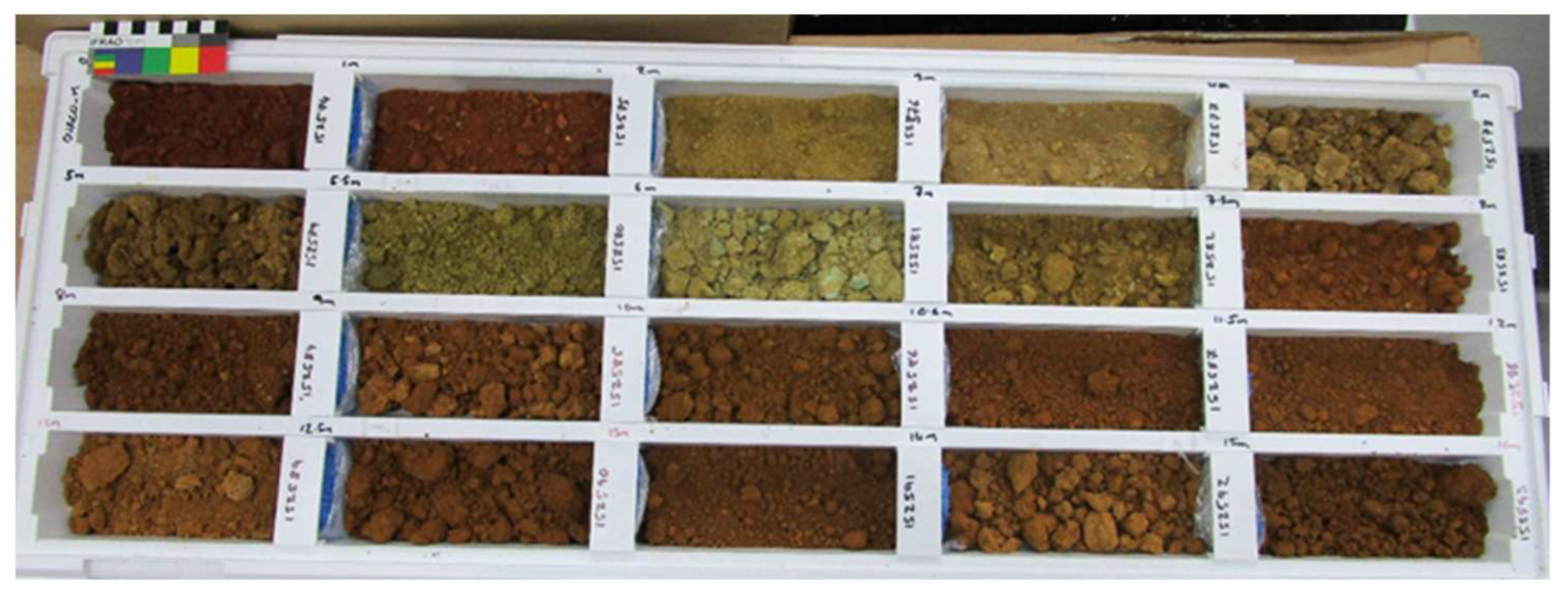
Nickel laterite ores represent over 60% of total nickel reserves; the remaining 40% is associated with nickel sulphide. New Caledonia is endowed with very large lateritic nickel deposits (Figure 1) that correspond to 11% of the nickel reserve worldwide with 6.7 Mt reserve and a production in 2019 of 280,000 t [24]. Nickel laterite ores are the product of intensive deep weathering of ultramafic rocks under humid tropical conditions. The resulting thick lateritic mantle extends from the bedrock to the surface and includes distinctive layers of altered and weathered rock as shown in Figure 2. Lithological units may include: (1) fresh or, totally or partially serpentinised dunite and/or harzburgite that consist mainly of olivine, pyroxene and serpentine minerals such as lizardite, antigorite and chrysotile; (2) saprock where weathering begins; (3) coarse saprolite with Ni-rich garnierite; (4) yellow laterite where Ni-goethite is dominant; (5) red laterite with a mixture of Ni-goethite and Ni-hematite and (6) lateritic duricrust [25]. In New Caledonia, the nickel mineralisation occurs as “oxide type” mainly in iron and manganese oxides or as “garnierite” type in Mg-Ni-silicates (Figure 2).
At present, logging of drill core is conducted by visual examination of the core by geologists, which results in subjective logging of lithological boundaries. The nickel laterite companies of New Caledonia have developed an ore type classification based on lithology, degree of serpentinisation and intensity of weathering (Table 1). Classification is dependent on mineral percentages estimated by the logging geologist. The lithology classification is based on the proportion of olivine and pyroxene as follows: if the proportion of olivine is more than 90%, it is dunite; otherwise, the label depends on the proportion of pyroxene. Harzburgite is 10 to 60% pyroxene, and pyroxenite is >60% pyroxene. Five serpentinization classes have been characterised (1) Superior (S) with 1–15% serpentine; (2) Intermediary (I) with 15–45% serpentine; (3) Normal (N) with 45–70% serpentine; (4) Basal (B) with 70–100% serpentine and (5) Green (Vert–V) with 45–70% serpentine (in this facies, the serpentinisation of the peridotites precedes the obduction). The degree of weathering is categorised from 0 to 5 based on the rock hardness and the presence of iron oxides (0 indicating no weathering and 5 indicating complete weathering).
The ability to develop a method for the collection of objective mineralogical data coupled with consistent lithological interpretation (including the identification of different ore types) would be of great value for the mining companies. Given that measurements of lateritic nickel diamond cores and drill chips demonstrated that the Corescan Hyperspectral Core Imager Mark III (HCI-3) could identify all the minerals present in the lateritic profile [21], it is proposed that the reflectance spectra can provide sufficient data for precise, objective, primary and alteration lithology and weathering boundary detection when used as input to an automated boundary detection algorithm.

2.1. Samples

All the samples used for this study were provided by the Nickel Mining Company (NMC). The samples were collected from the deposits of Boulinda Monique, N’Go and Ouaco Mousquetaire. NMC has generally a sampling density of 1 m for drill chip with some exceptions with denser sampling. A representative sub-sample of each 1 m drill chips sample was transferred in a 20 cm core tray compartment (Figure 3) before been measured with the imaging spectrometer.

2.2. Spectral Collection

Corescan’s HCI-3 combines reflectance spectroscopy, visual imagery and 3D laser profiling to map the mineralogy and geochemistry of geological samples. HCI-3 covers the VNIR (450 to 1300 nm) and SWIR (1300 to 2500 nm) range of the electromagnetic spectrum from 450 nm to 2500 nm at a spectral resolution (FWHM) of 3.5 nm. High quality optics focus the spectral measurement to a 0.5 mm point on the core. A RGB camera provides a high-resolution visual record of the core at 60 µm pixel size. Measurement of core surface features, texture and shape is complemented using a 3D laser profiler with a surface profile resolution of 20 µm. The system comprises a scan unit housing the optics, spectrometers, cameras and 3D profiling sensors; a translation table with conveyor driven core tray loading system and a high-speed data acquisition, processing and control computer. For each compartment sample, an average of 20,000 0.5 mm × 0.5 mm pixels were collected (depending on sample size) with an individual spectrum in each pixel. For this study, all the spectra from all pixels were averaged into 1 spectrum representing each sample.

2.3. Spectral Analysis

The HCI-3 can spectrally image drill core and cuttings at 0.5 mm resolution, hence providing distinct advantages by capturing pixels with less phases. Mineral mapping is undertaken using in-house proprietary expert system software. The reflectance spectrum in each pixel is either a pure mineral or a combination of two or more minerals; it is called a mineral class. For each mineral class, unique spectral indices were developed and consist of three parameters; (1) feature tracking that focuses on regions where absorptions exist; (2) matching regions that focuses on specific spectral regions and compare with the in-house database using Pearson correlation coefficient PCC and (3) spectral ratio which is a ratio of two reflectance values at specific wavelengths. Using the expert system, each pixel was mineralogically quantified and an average mineralogy for each sample was calculated.

3. Methods

The mathematical method described in this paper consists of three steps (Figure 4): (1) generating a 2D similarity matrix for the series of measurements in each drill hole; (2) converting the similarity matrix to a recurrence plot by applying a threshold, and (3) applying the quadrant scan method to the recurrence plot to generate a one-dimensional drill hole profile. Each of these three steps is described in detail in this section.
In the field of nonlinear time series analysis, recurrence is a fundamental characteristic of many dynamical systems. Recurrence is defined when two states of the system pass close to each other in phase space at different times. For example, in geology, recurrence occurs when geological processes produce similar (but not necessarily exactly the same) rock types because the geological processes are repeated over time. The recurrence plot was developed to reconstruct a time series as a two-dimensional plot to facilitate visual investigation of the recurrence structure in a system. This means that it can reduce any number of variables to a 2D representation (based on a similarity matrix), providing a very powerful dimensionality reduction tool. For example, a recurrence plot for drill hole data will indicate when similar rock types occur at different levels in the drill hole and where changes in rock type occur. Several measures have been developed to quantify features in recurrence plots, these are called recurrence quantification analysis measures (RQA). RQA measures can be used for quantitative investigation of the system’s properties and used to assess its dynamics. The recurrence plot and RQA measures are widely used as a time series analysis tool in many applications, including engineering [26], physics [27], chemistry [28], finance [29] and geology [15,30], and [31] provide an overview of the method and its applications to different systems.
Recently, a new RQA method was developed to identify transition points in time series data from dynamical systems, namely, the quadrant scan method [16,18,19]. It has been used in medical applications for the interpretation of Electroencephalography (EEG) and Electrocardiography (ECG) signals [18]. More recently, it has been demonstrated that the quadrant scan method can be applied to spatial data by replacing the time index with a spatial index when used to detect geological boundaries in geochemical and petrophysical data from drill holes [19]. These applications have demonstrated that the quadrant scan is capable of detecting points of change in a data series for both univariate and multivariate data. For application to drill hole data, an index that provides the order of sampling down hole is used. If sampling occurs at regular intervals, then this index can be replaced by the actual depth measurements. For irregularly sampled data, the depth index can be used to avoid having to resample the data at regular intervals, as is the case for boundary detection methods involving wavelet transforms. The computational efficiency and low computational cost of the quadrant scan method [19] makes it an attractive tool to identify domaining boundaries from high-dimensional hyperspectral data.
The quadrant scan method has two versions, standard (density) or weighted quadrant scan. As elaborated in [18,19], the steps of the standard version are outlined in the flowchart (Figure 4) and summarised in the following paragraphs.
(1)
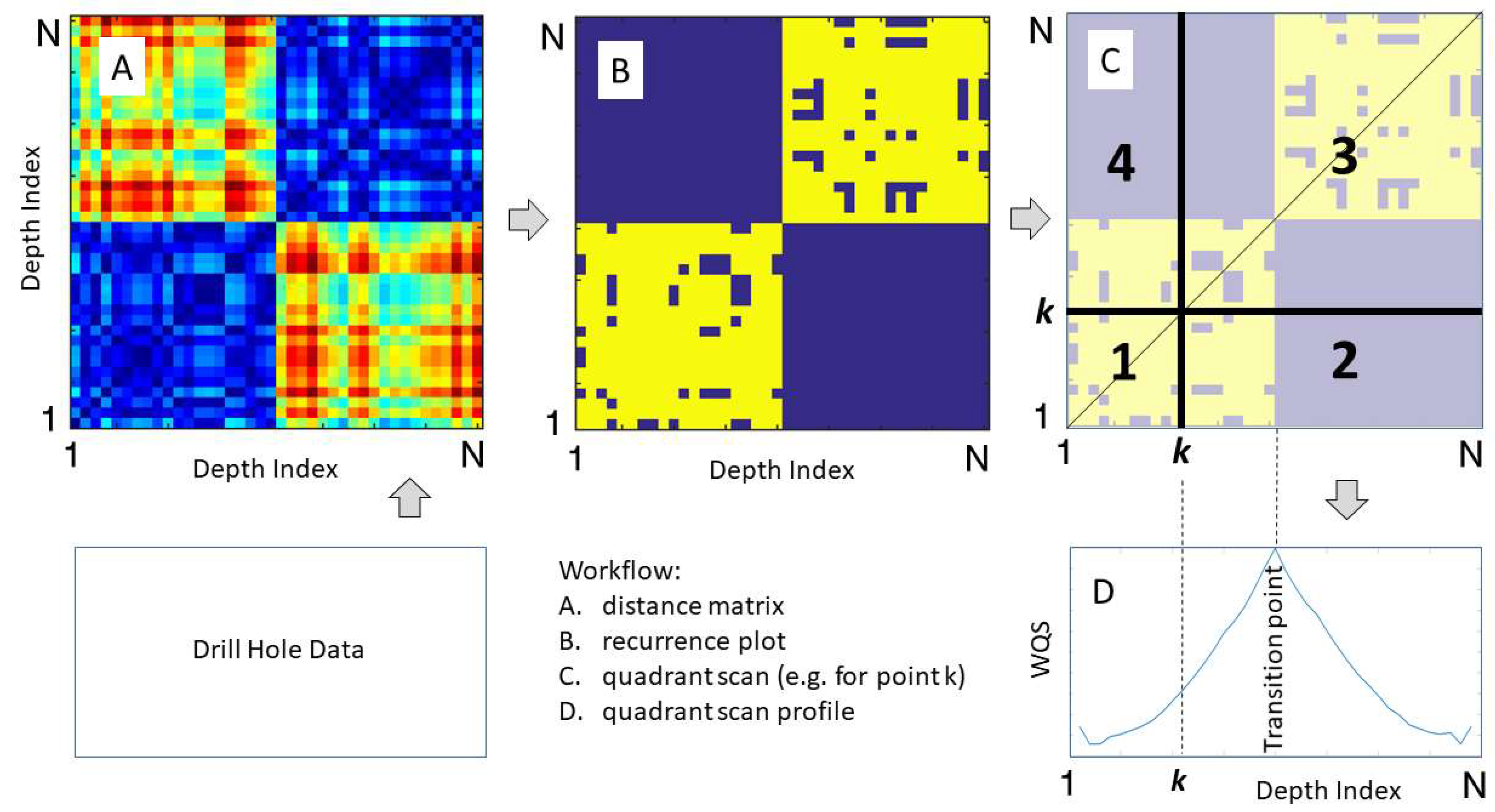
First, a distance matrix is constructed (Figure 4A). Generally, the Euclidian norm is used to measure the pairwise distance between two states of the system. However, because of the unique structure and high dimensionality of the spectral data, the Euclidian norm was found to be an inappropriate and misleading measure due to correlations in the hyperspectral data. The Mahalanobis distance was found to be more appropriate, as it can account for correlations in the data [32]. However, due to the significant difference in the dimensionality between the number of the variables and the number of samples, finding the inverse of the covariance matrix is problematic. Alternatively, we can find the distance using the covariance matrix of the normalised samples. Using this method has the advantage that it is not necessary to have a separate dimensionality reduction step, before constructing the distance matrix. Equivalent to the Mahalanobis distance, the distance matrix is defined as follows:
A i j = | | x ( i )   , x ( j ) | | = ( x ( i ) x ( j ) ) T S ( x ( i ) x ( j ) )  
where x ( d )     514 is a spectrum profile at depth with index d (e.g., i and j refer to different depth indices), while S is the covariance matrix of the normalised data. Each index in the matrix refers to the index of the sample, i.e., the depth index. Hence, the matrix width and height are determined by the total number of samples.
(2)
The recurrence plot matrix (Figure 4B) is constructed from the distance matrix A , by applying a threshold. If an entry in the distance matrix is less than the threshold, then the corresponding entry in the recurrence plot matrix is assigned to 1, otherwise it is 0. The threshold is controlled by a parameter α , which allows the user to control the scale of boundary detection [18,19]; that is, if α is small then the distance threshold will be small, which means that samples have to be very similar in composition to be considered below the threshold. The recurrence plot matrix and the threshold are defined as follows:
R i j = { 1 ,                 i f   a i j < ϵ   0 ,                 o t h e r w i s e
where
ϵ = α ( μ ( A i j ) + 3   σ ( A i j ) ) ; 0 < α < 1
where μ ( A i j ) and σ ( A i j ) are the mean and standard deviation of the distance matrix entries and ϵ is the threshold.
(3)
The quadrant scan profile (Figure 4D) is derived from the ratio of points in the binary recurrence plot above and below each depth index, by using the depth index to divide the recurrence plot into quadrants, as illustrated in Figure 4C. If D 1 , 3 and D 2 , 4 denote the density of the recurrent points in the first and third quadrants and the second and fourth quadrants, respectively, then the standard quadrant scan at depth index d for d = 1 , ,   N is defined as follows:
Q S ( d ) = D 1 , 3 D 1 , 3 + D 2 , 4
where, D 1 , 3 = i , j < d R i j + i , j > d R i j ( d 1 ) 2 + ( N d ) 2 and D 2 , 4 = i d ,   j d R i j + i > d ,   j < d R i j 2 ( d 1 ) ( N d ) .
In [19] a weighting scheme was applied in which higher weights were assigned to the states closer to the indexed point; this is called the weighted quadrant scan (WQS) method and showed considerable improvement over the standard quadrant scan method where all points are weighted equally. WQS requires two weighting parameters, m 1 and m 2 , to determine the smoothness of the weighting scheme and selection of these is problem dependent [18]. The result of the WQS method is a profile in which the peaks can be used to identify the transitions (Figure 4D). The WQS provides a reduction of the 514 values in the original spectrum to a single value for each sample. When applied to hyperspectral data, the peaks in the WQS profile are used to identify the locations of lithological boundaries. Sharp peaks indicate rapid transitions and rounded peaks represent more gradual transitions [18].
As explained above, the implementation of the WQS method requires the setting of three parameters α ,   m 1 and m 2 . Generally, as demonstrated in previous works, setting these parameters is problem dependent; however, guidance on how to choose these parameters and their effects on the WQS performance is discussed in [18]. Briefly, α adjusts and controls the recurrence threshold based on the distribution of the norm matrix and allows for multi-scale detection. The weighting scheme parameters m 1 and m 2 identify the gradient of the weighting function as well as the sizes of the neighbourhoods of the index point. Accordingly, the points within these neighbourhoods are assigned with maximum, transitional, or minimum weight. Finally, to avoid any artifact peaks in the WQS at the top or the bottom of any dataset which do not represent changes in the geological composition, the datasets are extended by copying the first and last samples four times.

4. Results

To test the algorithm, the WQS detection algorithm was applied to data from three drill-holes, namely OUACO, NGO_PB4 and BOULINDA. It is proposed that by using the reflectance spectra as input to the automated boundary detection algorithm, we can precisely and objectively detect boundaries for primary lithology, alteration or weathering where these are marked by changes in the spectra. For all the analyses, the weighting parameters were set at m 1 = 10 and m 2 = 2 ; this selection is based on the small number of the data samples, i.e., less than 50 samples per hole. The recurrence plot threshold was set at α = 0.03 ,   0.02   and   0.01 . The selection of these values is dependent on the distributions of the norm matrices derived by the Mahalanobis-like norms (Equation (3)). For spectral data, the largest variation of the WQS occurs when the value of α is within this range. For α < 0.01 and α > 0.03 there is less variation in the results. Therefore, we choose these values to demonstrate the robustness of our method. The variation of α allows detection of boundaries at different scales. In order to demonstrate the effectiveness of the WQS analysis for finding geological boundaries, we compare the results using a common unsupervised clustering technique, k-means [33]. K-means was chosen as it is very computationally efficient and one of the few clustering algorithms capable of handling such high dimensional data. To determine the optimal number of clusters for the k-means method, the Bayesian Information Criterion (BIC) [34] and the Elbow method are used [35] (Figure 5). The Elbow method plots the Residual Sum of Squares error (RSS) as a function of different values of k (the number of clusters), the optimal value of k is the point with most curvature. The BIC test penalizes for the number of clusters in addition to the RSS error; the minimal value of BIC identifies the optimal number of clusters. Figure 5 suggests that k = 8 is the optimal number of clusters to be used.
The results for the three drill-holes are illustrated in Figure 6, Figure 7 and Figure 8. Producing these results is quite fast; for example, generating a WQS profile from a 514-dimensional spectrum with 49 depth samples took approximately 6 s, including plotting three figures (the distance matrix, the recurrence plot matrix and the WQS profile), using MATLAB on a MacBook Pro. Figure 6a is a heat-map of the hyperspectral profiles at each depth interval in the OUACO hole (a total of 49 samples down hole). The heat-map is a graphical representation of spectral intensity down hole, wherein blue indicates low values and red indicates high values. Figure 6b shows the WQS profile derived from the spectral data using three different values of the parameter α (0.03, 0.02 and 0.01). The peaks in this curve identify the transition points in the data and, therefore, represent the predicted depth location of the lithological boundaries. Figure 6c demonstrates the results of the manual logging by domain experts; logging codes are described in Table 1. Figure 6d shows the results of the unsupervised k-means clustering technique. Figure 7 and Figure 8 show the same information as Figure 5, but for the other two drill holes, NGO_PB4 and BOULINDA.
The depth sampling intervals are irregular; therefore, the figures in this manuscript show the results in terms of depth indices. The corresponding actual depths are shown for each hole in Table 2.

5. Discussion

5.1. Comparison with Geologist Logging

Geological logs are plotted alongside the spectral analysis in Figure 6, Figure 7 and Figure 8 (panels c). There are three types of geological parameters in the logs: lithology, serpentinisation and weathering. Logging codes are decoded in Table 1 and, for example, a sample at depth index 4 will be coded as HI3 in Ouaco (Figure 6), whereas a sample at depth index 27 in NGO-PB4 will be coded as DB1 (Figure 7) and, lastly, a sample at depth index 26 will be coded HV1 at Boulinda (Figure 8). Caution must be exercised when comparing geological logs to logs derived from sensor data, such as hyperspectral imaging, because the input data to the two methods are not the same. For example, it would be unrealistic to expect hyperspectral data to recognise textural change that is not accompanied by mineralogical change. In addition, hyperspectral data may be able to distinguish changes in mineralogy that show no obvious visual change, and so will not be logged by the geologist.
Under lateritic conditions, the primary ultramafic rocks (dunite and harzburgite) are intensely serpentinised and weathered. The serpentinization (lizardite, nepouite) occurs first, affecting both olivine and pyroxene followed by the occurrence of weathering silicate minerals such as smectite and garnierite. The last and more intense weathering phase produces iron oxides such as goethite and hematite. Therefore, logging of lithology is largely based on the geologist’s interpretation of textures, such as grain pseudomorphs, to indicate the primary rock lithology. Hence, there is a low expectation that WQS analysis of the hyperspectral data will indicate primary lithological boundaries within the ultramafic rocks. Additionally, when the rock is intensely weathered (e.g., with degree 5), the goethite/hematite-goethite will dominate, as all other mineralogy have disappeared, and the WQS analysis of the hyperspectral data will distinguish boundaries between the laterite and less weathered rocks such as Ouaco at depth index 2 and 9 (Figure 6), NGO_PB4 at depth index 20 and 23 (Figure 7) and Boulinda at depth index 5 (Figure 8).
WQS also detect boundaries between serpentinisation I and V at depth index 24 as well as serpentinisation I and N at depth index 47 for Ouaco (Figure 6). At NGO_PB4 (Figure 7), significant peaks mark the boundaries between two types of laterite, for example, between LR and LI at depth index 5, between LI and LT at depth index 19, and at depth index 20 between LT and BS. Additionally, boundaries were detected between serpentine N and B (depth index 23) and lithology H and D (depth index 31) and weathering 2 and 3 (depth index 39). At Boulinda, boundaries were identified between dunite (D) and harzburgite (H) and weathering 2 and 4 (depth index 8), between lithology H and D, serpentine V and B and weathering 2 and 3 (depth index 15), between lithology D and H and weathering 2 and 3 (depth index 23) and between weathering 2 and 3 (depth index 29). However, it is difficult to confidently assign any profile peaks to the different ultramafic rocks, and this is likely due to their altered and weathered state. It is often the case that boundaries for alteration and weathering are gradational and the distinction between the different groups (strong to weak) is highly subjective when logged by geologists. It is for these cases that the use of non-subjective methods can be most useful. The WQS technique can be used to identify significant changes in the cores that are difficult to pinpoint using manual identification. A more detailed investigation of the mineralogy and the core would be required to distinguish between these options. The value in the WQS technique is that it highlights these changes in the mineralogy, which might otherwise be missed by the logging geologist. It is also the case that some of these changes are occurring in parts of the hyperspectral bandwidth that do not provide useful information for geological logging. As previously mentioned, the detection of olivine and pyroxene can only be detected if the weathering is not intense, as iron oxides will mask their diagnostic features in the visible and near infrared part of the electromagnetic spectrum.

5.2. Comparison with k-Means Clustering

Panels (b) and (d) of Figure 6, Figure 7 and Figure 8 compare the boundary identification results derived by the implementation of WQS with the samples classes derived from k-means clustering (for k = 8 clusters as suggested by the BIC and the Elbow method tests in Figure 5), respectively, on the high dimensional spectral data. K-means failed to distinguish important lithological boundaries, instead it provides many lithological boundaries based on changes in sample composition, which may be small or large. K-means attempts to divide a data set into approximately spherical clusters of approximately equal size. If the data structure is not compatible, then the class boundaries may be fairly arbitrary. Therefore, the change in class label may be due to arbitrary subdivision of the data into clusters, and may not signify an important change in composition. Because the WQS method takes the spatial correlation of the data into account, it is able to indicate where the more and less significant changes are using the peak height. Using the WQS method, we can be confident that the large peaks indicate significant change in the rock composition has occurred.

5.3. Comparison with the Spectrally Derived Mineralogy

Using the Corescan expert system, each pixel was mineralogically quantified and an average mineralogy for each sample was calculated. The results of this calculation are shown in Figure 9, Figure 10 and Figure 11 as abundance percentages of the minerals. More detailed information on the analysis of the spectral mineralogy will be available in a forthcoming paper and, therefore will not be addressed further here. To understand how the boundaries detected by the WQS using the spectral data correspond to mineralogical changes the abundance ratio of the minerals is plotted alongside the spectral analysis in Figure 9, Figure 10 and Figure 11.
For Ouaco (Figure 9), the WQS peaks indicate that the most significant changes in the mineralogy in the upper part of the profile are mainly depend on goethite, goethite-hematite and all the types of the smectite percentages. Toward the base of the profile, the main mineralogical variations are based on smectite derived from serpentine, lizardite and weathered serpentine percentages. These changes occur, respectively, (a) at depth index 2, with an increase in goethite-hematite (goethite dominant) and hematite-goethite (hematite dominant) percentages; (b) at depth index 9, with an increase in goethite and Mg-smectite percentages and a decrease in Mg-Ni smectite; (c) at depth index 25 with a decrease in Mg smectite percentage; (d) at depth index 29 with a decrease in Mg smectite percentage; (e) at depth index 37 with an increase in smectite serpentine percentage, and (f) at depth index 47 with an increase in smectite serpentine, lizardite and weathered serpentine percentages and a decrease in Mg smectite percentage.
For NGO_PB4 (Figure 10), the boundaries at depth index, 5, 11 and 15 correspond to a relative change between goethite and goethite-hematite abundance. The boundaries identified at depth index 20 correspond to a decrease in goethite percentage and an increase in weathered serpentine percentage whereas depth index 23 is linked to an increase in lizardite. The small change at depth index 27 correspond to a small goethite increase, while variation at depth index 31 indicates a large goethite increase with an equivalent weathered serpentine percentage decrease. The last change at depth index 39 is due the presence of a small amount of smectite derived from serpentine.
Similar observations can be made for boundaries detected in the Boulinda drill-hole (Figure 11). The different detection scales (α values) provide complementary results. The boundaries at depth indices at 3, 5, 8, 10, 13, 15, 20, 23, 25, 27, 29 and 30 all correspond to observable changes in mineral abundances for the iron oxides in the upper part of the profile, for weathered serpentine, smectite serpentine, lizardite and népouite, serpentine derived from olivine and serpentine derived from orthopyroxene in the lower part of the profile.

5.4. Precision of Boundary Detection and Dependance on Sample Size

For automated methods, the precision of boundary detection depends on the sampling interval. For boundary detection methods based on the continuous wavelet transform, a consistent size sampling interval is required and, therefore, if the data are provided at varying scales, all data must be re-scaled to the same scale resulting in a loss of information. This is not the case for WQS. For this study, most of the sampling intervals were approximately one metre (Table 2). However, for a large section of the BOULINDA hole, the sampling interval was much smaller. Using WQS automatically allows a more precise identification of boundary location in this section of the drill hole.
The user needs to take the sampling interval into account when interpreting the results, especially in the case where the sample size is not consistent down hole, as this affects the precision of the boundary location. Additionally, the spatial correlation depends on the number of samples not the length they occupy in the drill hole.

6. Conclusions

The WQS, based on the recurrence plot, allows identification of boundaries between geological domains from very high-dimensional data. The method has been tested on spectral data from three different drill-holes. The advantages of this algorithm are: (1) it is automated and so provides consistent data analysis and repeatable results; (2) it is computationally efficient and can be calculated quickly using a standard desktop or laptop computer; (3) the algorithm is unsupervised and does not require any geological knowledge; (4) it reduces very high dimensional spectral data (D = 514) into a single dimension, i.e., the WQS profile, in which the peaks identify the lithological boundaries; (5) the significance of the boundary can be inferred from the peak height; (6) sample intervals do not have to be of consistent size and localised finer scale sampling produces more precise results. This is beneficial for geologists and geological applications as it provides rapid results and indicates to the geologist the locations of significant changes in the geology based on the data.

Author Contributions

Conceptualization, A.Z., E.R. and J.H.; methodology, A.Z., D.M.W. and M.S.; software, A.Z.; validation, A.Z., E.R., J.H., D.M.W. and M.S.; formal analysis, A.Z.; investigation, A.Z., E.R., J.H., D.M.W. and M.S.; resources, E.R. and J.H.; data curation, E.R.; writing—original draft preparation, A.Z., E.R. and J.H.; writing—review and editing, A.Z., E.R., J.H., D.M.W. and M.S. All authors have read and agreed to the published version of the manuscript.

Funding

A.Z. is supported by the Australian Research Council through the Centre for Transforming Maintenance through Data Science (grant number IC180100030), funded by the Australian Government. A.Z. and M.S. acknowledge the support of the Australian Research Council through the Discovery Grant DP 180100718. D.M.W. and M.S. are partially supported by the Australian Research Council (DP200102961).

Conflicts of Interest

The authors declare no conflict of interest.

Computer Code and Software

The MATLAB code for the WQS method is available in the following public GitHub repository https://github.com/AyhamZaitouny/Boundaries-Detection-Weight-Quadrant-Scan- (accessed on 7 October 2021). For more information, contact the corresponding author.

References

  1. Singh, H.; Seol, Y.; Myshakin, E.M. Automated Well-Log Processing and Lithology Classification by Identifying Optimal Features Through Unsupervised and Supervised Machine-Learning Algorithms. SPE J. 2020, 25, 2778–2800. [Google Scholar] [CrossRef]
  2. Hill, E.J.; Pearce, M.A.; Stromberg, J.M. Improving Automated Geological Logging of Drill Holes by Incorporating Multiscale Spatial Methods. Math. Geol. 2021, 53, 21–53. [Google Scholar] [CrossRef] [Green Version]
  3. Hill, E.; Robertson, J.; Uvarova, Y. Multiscale hierarchical domaining and compression of drill hole data. Comput. Geosci. 2015, 79, 47–57. [Google Scholar] [CrossRef]
  4. Marr, D.; Hildreth, E. Theory of edge detection. Proc. R. Soc. Lond. Ser. B Biol. Sci. 1980, 207, 187–217. [Google Scholar]
  5. Canny, J. A computational approach to edge detection. IEEE Trans. Pattern Anal. Mach. Intell. 1986, 6, 679–698. [Google Scholar] [CrossRef]
  6. Mallat, S. Zero-crossings of a wavelet transform. IEEE Trans. Inf. Theory 1991, 37, 1019–1033. [Google Scholar] [CrossRef]
  7. Perez-Muñoz, T.; Velasco-Hernandez, J.; Hernandez-Martinez, E. Wavelet transform analysis for lithological characteristics identification in siliciclastic oil fields. J. Appl. Geophys. 2013, 98, 298–308. [Google Scholar] [CrossRef]
  8. Cooper, G.R.J.; Cowan, D.R. Blocking geophysical borehole log data using the continuous wavelet transform. Explor. Geophys. 2009, 40, 233–236. [Google Scholar] [CrossRef]
  9. Davis, A.C.; Christensen, N.B. Derivative analysis for layer selection of geophysical borehole logs. Comput. Geosci. 2013, 60, 34–40. [Google Scholar] [CrossRef] [Green Version]
  10. Arabjamaloei, R.; Edalatkha, S.; Jamshidi, E.; Nabaei, M.; Beidokhti, M.; Azad, M. Exact lithologic boundary detection based on wavelet transform analysis and real-time investigation of facies discontinuities using drilling data. Pet. Sci. Technol. 2011, 29, 569–578. [Google Scholar] [CrossRef]
  11. Walker, D.M.; Zaitouny, A.; Corrêa, D.C. On using the modularity of recurrence network communities to detect change-point behaviour. Expert Syst. Appl. 2021, 176, 114837. [Google Scholar] [CrossRef]
  12. Goswami, B. A Brief Introduction to Nonlinear Time Series Analysis and Recurrence Plots. Vibration 2019, 2, 332–368. [Google Scholar] [CrossRef] [Green Version]
  13. Goswami, B.; Boers, N.; Rheinwalt, A.; Marwan, N.; Heitzig, J.; Breitenbach, S.F.M.; Kurths, J. Abrupt transitions in time series with uncertainties. Nat. Commun. 2018, 9, 48. [Google Scholar] [CrossRef]
  14. Aminikhanghahi, S.; Cook, D.J. A survey of methods for time series change point detection. Knowl. Inf. Syst. 2017, 51, 339–367. [Google Scholar] [CrossRef] [Green Version]
  15. Marwan, N.; Carmenromano, M.; Thiel, M.; Kurths, J. Recurrence plots for the analysis of complex systems. Phys. Rep. 2007, 438, 237–329. [Google Scholar] [CrossRef]
  16. Rapp, P.E.; Darmon, D.M.; Cellucci, C.J. Hierarchical Transition Chronometries in the Human Central Nervous System. IEICE Proc. Ser. 2013, 2, 286–289. [Google Scholar] [CrossRef]
  17. Walker, D.M.; Tordesillas, A.; Ren, J.; Dijksman, J.A.; Behringer, R.P. Uncovering temporal transitions and self-organization during slow aging of dense granular media in the absence of shear bands. EPL Europhys. Lett. 2014, 107, 18005. [Google Scholar] [CrossRef]
  18. Zaitouny, A.; Walker, D.M.; Small, M. Quadrant scan for multi-scale transition detection. Chaos Interdiscip. J. Nonlinear Sci. 2019, 29, 103117. [Google Scholar] [CrossRef]
  19. Zaitouny, A.; Small, M.; Hill, J.; Emelyanova, I.; Ben Clennell, M. Fast automatic detection of geological boundaries from multivariate log data using recurrence. Comput. Geosci. 2019, 135, 104362. [Google Scholar] [CrossRef] [Green Version]
  20. Wells, M.A.; Ramanaidou, E.R.; Verrall, M.; Tessarolo, C. Mineralogy and crystal chemistry of “garnierites” in the Goro lateritic nickel deposit, New Caledonia. Eur. J. Mineral. 2009, 21, 467–483. [Google Scholar] [CrossRef]
  21. Ramanaidou, E.; Fonteneau, L.; Sevin, B.; Foucher, W. Characterisation of New Caledonian nickel laterite using hyperspectral imaging. In Proceedings of the Australia Geological Council Convention, Adelaide, Australia, 14–18 October 2018. [Google Scholar]
  22. Cracknell, M.J.; Jansen, N.H. National Virtual Core Library HyLogging data and Ni-Co laterites: A mineralogical model for resource exploration, extraction and remediation. Aust. J. Earth Sci. 2016, 63, 1053–1067. [Google Scholar] [CrossRef]
  23. Cardoso-Fernandes, J.; Silva, J.; Perrotta, M.M.; Lima, A.; Teodoro, A.C.; Ribeiro, M.A.; Dias, F.; Barrès, O.; Cauzid, J.; Roda-Robles, E. Interpretation of the Reflectance Spectra of Lithium (Li) Minerals and Pegmatites: A Case Study for Mineralogical and Lithological Identification in the Fregeneda-Almendra Area. Remote Sens. 2021, 13, 3688. [Google Scholar] [CrossRef]
  24. USGS. Science for a Changing World. National Minerals Information Center. 2021. Available online: https://www.usgs.gov/centers/national-minerals-information-center/nickel-statistics-and-information (accessed on 7 October 2021).
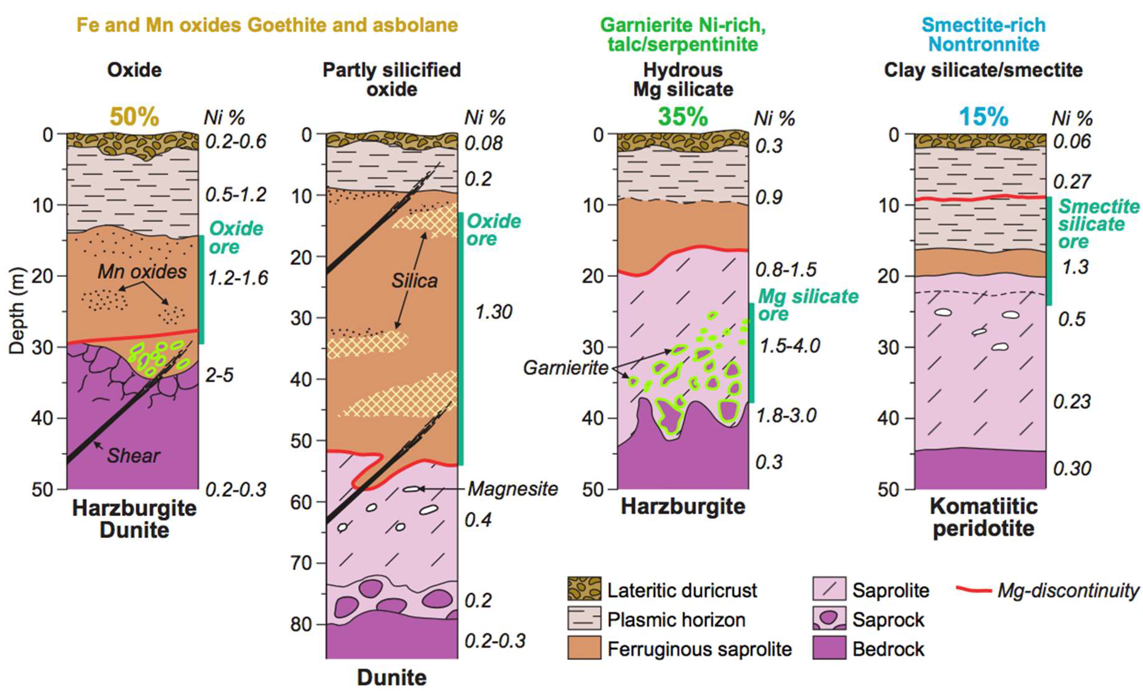
  25. Butt, C.R.; Cluzel, D. Nickel laterite ore deposits: Weathered serpentinites. Elements 2013, 9, 123–128. [Google Scholar] [CrossRef]
  26. Elwakil, A.; Soliman, A. Mathematical Models of the Twin-T, Wien-bridgeand Family of Minimum Component Electronic ChaosGenerators with Demonstrative Recurrence Plots. Chaos Solitons Fractals 1999, 10, 1399–1412. [Google Scholar] [CrossRef]
  27. Vretenar, D.; Paar, N.; Ring, P.; Lalazissis, G.A. Nonlinear dynamics of giant resonances in atomic nuclei. Phys. Rev. E 1999, 60, 308–319. [Google Scholar] [CrossRef] [PubMed] [Green Version]
  28. Rustici, M.; Caravati, C.; Petretto, E.; Branca, M.; Marchettini, N. Transition Scenarios during the Evolution of the Belousov−Zhabotinsky Reaction in an Unstirred Batch Reactor. J. Phys. Chem. A 1999, 103, 6564–6570. [Google Scholar] [CrossRef]
  29. Gilmore, C.G. Detecting Linear and Nonlinear Dependence in Stock Returns: New Methods Derived from Chaos Theory. J. Bus. Financ. Account. 1996, 23, 1357–1377. [Google Scholar] [CrossRef]
  30. Marwan, N.; Thiel, M.; Nowaczyk, N.R. Cross recurrence plot based synchronization of time series. Nonlinear Process. Geophys. 2002, 9, 325–331. [Google Scholar] [CrossRef]
  31. Marwan, N. A historical review of recurrence plots. Eur. Phys. J. Spec. Top. 2008, 164, 3–12. [Google Scholar] [CrossRef] [Green Version]
  32. De Maesschalck, R.; Jouan-Rimbaud, D.; Massart, D.L. The mahalanobis distance. Chemom. Intell. Lab. Syst. 2000, 50, 1–18. [Google Scholar] [CrossRef]
  33. Jain, A.K. Data clustering: 50 years beyond K-means. Pattern Recognit. Lett. 2010, 31, 651–666. [Google Scholar] [CrossRef]
  34. Schwarz, G. Estimating the Dimension of a Model. Ann. Stat. 1978, 6, 461–464. [Google Scholar] [CrossRef]
  35. Ketchen, D.J.; Shook, C.L. The application of cluster analysis in strategic management research: An analysis and critique. Strateg. Manag. J. 1996, 17, 441–458. [Google Scholar] [CrossRef]
Figure 1. Location of the peridotites and the nickel deposits of New Caledonia [20].
Minerals 12 00049 g001
Figure 2. Typical weathering profiles developed on ultramafic rocks with absolute and residual accumulation of Ni and Co (Modified from [25]).
Minerals 12 00049 g002
Figure 3. Drill chips from OUACO deposit prepared in a core tray divided into 20 cm compartments.
Minerals 12 00049 g003
Figure 4. A flowchart demonstrating the steps of the proposed mathematical method. In subplot (A), the colours represent the difference between each sample and all other samples in the drill hole using the multivariate data. For the binary recurrence matrix, in subplot (B), blue represents 0 (above the threshold) and yellow represents 1 (below the threshold). At each depth index, the recurrence matrix is divided into four quadrants, shown in subplot (C), the black vertical and horizontal lines demonstrate the division for depth index k. The ratio of quadrant values transforms the 2D plot into a simple function, subplot (D), where maxima indicate transition points in the input data.
Minerals 12 00049 g004
Figure 5. Tests to determine the optimal number of clusters for the k-means method. (a) The Bayesian Information Criterion (BIC) test shows that 8 is the optimal number of clusters at which the testing criterion is minimal, and; (b) The Elbow method test: it shows the Residual Sum of Squares error (RSS) as a function of the number of clusters.
Minerals 12 00049 g005
Figure 6. OUACO drill-hole. (a) Heatmap plot of depth index against spectral index (blue colours reflect low values and red colours reflect high values); (b) Weighted quadrant scan results from the spectral data using three different values of α , peaks indicate lithological boundaries; (c) The boundaries identified manually by domain experts (see Table 1 for geology logging codes), and; (d) Results of k-means clustering with k = 8 (the different colours represent different clusters).
Minerals 12 00049 g006
Figure 7. NGO_PB4 drill-hole. (a) Heatmap plot of depth index against spectral index (blue colours reflect low values and red colours reflect high values); (b) Weighted quadrant scan results from the spectral data using three different values of α , peaks indicate lithological boundaries; (c) The boundaries identified manually by domain experts (see Table 1 for geology logging codes), and; (d) Results of k-means clustering with k = 8 (the different colours represent different clusters).
Minerals 12 00049 g007
Figure 8. BOULINDA drill-hole. (a) Heatmap plot of depth index against spectral index (blue colours reflect low values and red colours reflect high values); (b) Weighted quadrant scan results from the spectral data using three different values of α , peaks indicate lithological boundaries; (c) The boundaries identified manually by domain experts (see Table 1 for geology logging codes), and; (d) results of k-means clustering with k = 8 (the different colours represent different clusters).
Minerals 12 00049 g008
Figure 9. OUACO drill-hole: The WQS analysis in comparison with the abundance percentage of different minerals obtained with Corescan. The left panel is the WQS results from the spectral data using three different values of α , peaks indicate lithological, alteration and weathering boundaries. The rest of the panels show the abundance percentage of different minerals along the drill-hole.
Minerals 12 00049 g009
Figure 10. NGO_PB4 drill-hole: The WQS analysis in comparison with the abundance percentage of different minerals obtained with Corescan. The left panel is the WQS results from the spectral data using three different values of α , peaks indicate lithological, alteration and weathering boundaries. The rest of the panels show the abundance percentage of different minerals along the drill-hole.
Minerals 12 00049 g010
Figure 11. BOULINDA drill-hole: The WQS analysis in comparison with the abundance percentage of different minerals obtained with Corescan. The left panel is the WQS results from the spectral data using three different values of α , peaks indicate lithological, alteration and weathering boundaries. The rest of the panels show the abundance percentage of different minerals along the drill-hole.
Minerals 12 00049 g011
Table 1. Interpretation of geological domaining samples.
Laterite/Primary LithologySerpentinizationWeathering
Logging CodeInterpretationLogging CodeInterpretationLogging CodeInterpretation
LRLatérite Rouge
(Red Laterite)
NANot AssignedNANot Assigned
LJLatérite Jaune
(Yellow Laterite)
IIntermediary1Weak Weathering
LTLatérite de Transition (Transition Laterite)VVert (green)2
BSBasal SerpentineNNormal3
HHarzburgiteBBasal4
DDunite 5Strong weathering
HDHarzburgite/Dunite
DHDunite/Harzburgite
Table 2. The depth indices and corresponding actual depths in metres for each hole.
DEPTH INDEX12345678910111213141516171819202122232425
OUACO123455.5677.3891010.611.51212.5131415161718192021
NGO_PB40.31234567891011121314151617181919.2202121.522
BOULINDA11.323455.266.75788.38.68.89.19.49.610.210.811.31212.413.113.313.8
DEPTH INDEX26272829303132333435363738394041424344454647484950
OUACO2222.652324252627282930313233343536373838.639.640.34141.642_
NGO_PB422.52323.7524.7525.326272828.5293030.3323232.532.933.5________
BOULINDA141515.215.51617___________________
Publisher’s Note: MDPI stays neutral with regard to jurisdictional claims in published maps and institutional affiliations.

