Article

The Mixed-Layer Structures of Ikunolite, Laitakarite, Joséite-B and Joséite-A

1
School of Civil, Environmental and Mining Engineering, The University of Adelaide, Adelaide, SA 5005, Australia
2
School of Chemical Engineering and Advanced Materials, The University of Adelaide, Adelaide, SA 5005, Australia
3
Adelaide Microscopy, The University of Adelaide, Adelaide, SA 5005, Australia
4
BHP Olympic Dam, Adelaide, SA 5000, Australia
*
Author to whom correspondence should be addressed.
Minerals 2021, 11(9), 920; https://doi.org/10.3390/min11090920
Submission received: 11 July 2021 / Revised: 21 August 2021 / Accepted: 22 August 2021 / Published: 25 August 2021
(This article belongs to the Special Issue 10th Anniversary of Minerals: Frontiers of Mineral Science)

Abstract

:
We used high-angle annular dark field scanning transmission electron microscopy (HAADF STEM) to image the crystal structures of four minerals in the Bi4X3 isoseries (X = Te, Se, S), a subgroup of the tetradymite homologous series: ikunolite (Bi4S3), laitakarite (Bi4Se2S), joséite-B (Bi4Te2S), and joséite-A (Bi4TeS2). The four minerals are isostructural and interpretable in terms of regular stacking of seven-atom packages: [Bi–S–Bi–S–Bi–S–Bi], [Bi–Se–Bi–S–Bi–Se–Bi], [Bi–Te–Bi–S–Bi–Te–Bi], and [Bi–S–Bi–Te–Bi–S–Bi], respectively. The four phases are mixed-layer structures representing the Bi2kTe3 (k = 2) module within the tetradymite series. Diffraction patterns confirm they are seven-fold superstructures of a rhombohedral subcell with c/3 = d~1.89–1.93 Å. Modulation along the d* interval matches calculations of reflection intensity using the fractional shift method for Bi4X3. Internal structures can be discerned by high-resolution HAADF STEM imaging and mapping. Paired bismuth atoms are positioned at the outside of each seven-atom layer, giving the minerals a modular structure that can also be considered as being composed of five-atom (X–Bi–X–Bi–X) and two-atom (Bi–Bi) sub-modules. The presence of mixed sites for substituting cations is shown, particularly for Pb. Moreover, Pb may be important in understanding the incorporation of Ag and Au in Bi–chalcogenides. Visualisation of crystal structures by HAADF STEM contributes to understanding relationships between phases in the tetradymite homologous series and will play an invaluable role in the characterization of potential additional members of the series.

1. Introduction

The tetradymite homologous series is an extended family of named minerals, unnamed natural phases, experimentally synthesized products, and predicted mixed-layer structures with BixXy stoichiometry (X = S, Se, or Te) that can be related to the tetradymite (Bi2Te2S) archetype [1,2]. To derive a systematic homology for the series and predict structural arrangements for any stoichiometry, Ciobanu et al. [2] presented a structural model drawing on earlier work by many authors ([3,4,5,6,7,8], among others), in which layer stacks of different size are combined in various proportions.
This crystal-structural model in turn provides a crystal-structural framework for the series that can assist in the characterisation of new natural or synthetic phases without the requirement of single crystal diffraction studies, which are often impossible, or at least impractical, due to the characteristic nanoscale intergrowths and disordering among members of the series. Tetradymite and isostructural Bi2X3 phases such as tellurobismuthite, paraguanajuatite, kawazulite, and skippenite are represented by a single five-atom X–Bi–X–Bi–X layer. A defining feature of Bi-richer members of the tetradymite homologous series is, however, the presence of paired bismuth atoms (Bi–Bi) inserted at the edges of the five-atom layer and linked to one another by metallic bonds. Thus, a seven-atom layer is created in Bi4X3 species [Bi–X–Bi–X–Bi–X–Bi], a nine-atom layer, with double Bi–Bi pairs in Bi6X3 [Bi–Bi–X–Bi–X–Bi–X–Bi–Bi], and with tripled Bi–Bi pairs to form an eleven-atom layer in Bi8X3 species [Bi–Bi–Bi–X–Bi–X–Bi–X–Bi–Bi–Bi].
The mineralogy of the tetradymite homologous series is currently only incompletely documented. The literature contains reports of many unnamed or inadequately characterized species (see review in [1]), even though fitted structures can be predicted for a majority, if not all, of these species based on the aforementioned structural models. Synthetic compounds derived from tetradymite have also attracted attention from materials science researchers, due to characteristics that enable their use as thermoelectric devices and topological insulators ([9,10], and references therein). Like named minerals and other natural phases, synthetic products in the system Bi–Te (e.g., [11,12,13]) can also be interpreted in terms of different combinations and proportions of layers. This homology thus allows the derivation of a systematic group homology [1,2] and implies that each individual member of the series should be stoichiometric in composition. Lattice-scale intergrowths are, however, a common feature of the tetradymite group [e.g., [14]) and the related aleksite homologous series [15], leading to non-stoichiometric compositions being widely reported in the literature.
High angle annular dark field scanning transmission electron microscopy (HAADF STEM) represents a powerful technique to directly visualise the structures of modular mixed-layer compounds [16,17,18,19]. The technique takes advantage of the amplified Z contrast that highlights compositional differences between heavy atoms such as Bi, Pb, and Te, and is also best suited for visualizing large modular structures such as Pb–Bi-sulfosalts [20,21]. HAADF STEM has been successfully employed, for example, to reveal the three distinct polytypes of PbBi4Te4S3, a new member of the related aleksite homologous series [15].
Here, we use HAADF STEM imaging to confirm the arrangement of layers for four named minerals of the tetradymite homologous series with Bi4X3 stoichiometry (ikunolite, laitakarite, joséite-B and joséite-A). Furthermore, HAADF STEM imaging allows an understanding of the distribution of atoms within those layers.

2. Background: The Bi4S3–Bi4Se3–Bi4Te3 Isoseries

There are currently five named minerals in the Bi4S3–Bi4Se3–Bi4Te3 isoseries: ikunolite (Bi4S3), laitakarite (Bi4Se3), pilsenite (Bi4Te3), joséite-A (Bi4TeS2), and joséite-B (Bi4Te2S). Laitakarite has been defined as Bi4(Se, S)3 [22] and indeed, most published data show the presence of up to one atom per formula unit (a.p.f.u.) S alongside Se (Figure 8 in [1], and references therein). Based on compositional data from the Orijärvi deposit, southwest Finland, which showed a marked bimodal distribution [1], laitakarite was considered to most likely represent two distinct species: Bi4Se3 and Bi4Se2S. The tellurian laitakarite mentioned in the same publication is probably an additional species with the formula Bi4Se2Te. Other predicted species in the Bi4X3 isoseries include Bi4S2Se and Bi4S2Te. Natural ikunolite typically contains some Se, suggesting partial or complete solid solution series between Bi4S3 and Bi4S2Se.
The structures of three minerals in the Bi4S3–Bi4Se3–Bi4Te3 isoseries—pilsenite, laitakarite (Bi4Se3), and ikunolite—are shown in Figure 1. Note that all structures are composed of a five-atom submodule [X–Bi–X–Bi–X] and a second submodule comprising Bi–Bi atom pairs. Such a five- and two-atom model was first introduced by Imamov and Semiletov [4] for phases in the Bi–Se, Bi–Te and Sb–Te systems, with the term “compositional polytypism” suggested to underline the structural modularity of phases with variable compositions. This model was followed by Shelimova et al. [7] who suggested the structural formula nBi2·mBi2X3 for describing homology in layered tetradymite-like compounds in the systems Bi–Te and GeTe–Bi2Te3.
This two- and five-atom model was questioned by Frangis et al. [6], who considered the component modules to be formed by the addition of M–X (instead of M–M layers) to the Bi2X3 archetype. Based on HR TEM studies of compounds of the M2+δX3 type, where M = Bi, Sb, Ge, X = Te, Se, and 0 ≤ δ ≤ 0.4, Frangis et al. [6] describe a continuous series of one-dimensional, interface-modulated structures based on the model of Van Landuyt et al. [3]. Lind and Lidin [8] applied superspace formalism to phases in the system Bi–Se and derived a general model in which all structures are included within the 4D group P: R3:m 1 ¯ 1, with cell parameters a ~4.2 Å and csub ~5.7 Å. Their study was based on X-ray diffraction of phases in the compositional range Bi2Se3–Bi4Se3, extrapolated to Bi3Se2 (=Bi4.5Se3). A saw-tooth displacive modulation was considered for the interpretation of these structures.
Ciobanu et al. [2] considered the phases in the tetradymite series as mixed layer compounds with a general formula: S’ (Bi2kX3)∙L’ (Bi2(k+1)X3) (k ≥ 1; X = chalcogen; S’, L’ = number of short and long modules, respectively). This working model was based on the HR-TEM study of multiple phases in an extended compositional range Bi2Te3–Bi8Te3, showing that they are all an N-fold superstructure of a rhombohedral subcell with c/3 = d~0.2 nm, where N is the number of layers in the stacking sequence [2]. Electron diffraction (ED) patterns, displaying the two brightest reflections about the middle of d*, are described by a monotonic decrease of two displacive modulations with an increase in Bi content. Such displacements were quantified by fractional shifts between reflections in the derived and basic structures [2]. Mixed-layer compounds are a class of minerals in which ED patterns display characteristic features [5], which, if linked to a homology in a defined series of structures, can be used to predict the stacking sequence and chemistry of discrete phases.
As the series progresses towards Bi-rich compositions, compounds in the Bi4X3 isoseries represent the first structures defined by a single module (Bi2kX3; k = 2) in which single Bi–Bi pairs occur between the chalcogen-bearing, five-atom submodule, common to all phases in the series (Figure 1B).

3. Microanalytical Methodology

3.1. Electron Probe Microanalysis

Quantitative compositions were determined using a Cameca SX-Five electron probe microanalyzer (EPMA), equipped with five tuneable wavelength-dispersive spectrometers. The instrument runs PeakSite v6.5 software for microscope operation, and Probe for EPMA software (distributed by Probe Software Inc., Eugene, OR, USA) for all data acquisition and processing. Operating conditions utilized were 20 kV/20 nA with a focused beam.
The full list of elements analysed along with count times, nominal detection limits, and primary and interference standards are presented in Supplementary Materials, Tables S1–S3. Of particular note is the increased count time utilized for Au Lα for better detection limit. Matrix corrections of Armstrong-Love/Scott φ(ρz) [26] and Henke MACs were used for data reduction.
Traditional two-point backgrounds were acquired. Due to complex off-peak interferences in these sample matrices, the shared background function of Probe for EPMA was utilized. This function allows the collected background positions of elements on the same spectrometer be used for all elements on that spectrometer, allowing multipoint backgrounds to be applied to each element. However, in simple background regions, a traditional two-point linear fit was still used.
In addition, the first element acquired on each spectrometer (i.e., typically S, Te, Fe, Se, Zn) was analysed using the time dependent intensity (TDI) correction feature of Probe for EPMA (e.g., [27]). Using this method, the decay of X-ray counts over time is measured and modelled to return a t = 0 intercept, and from this a concentration is calculated. This minimizes the impact of element migration and can be reviewed, disabled, or enabled post analysis.

3.2. Nanoscale Analysis

Preparation of thinned (<100 nm) foils for TEM investigation from the polished blocks was performed using a FEI-Helios nanoLab dual-focused ion beam and scanning electron microscope (FIB-SEM), following procedures outlined by Ciobanu et al. [28]. Each TEM foil was attached to a copper grid.
Foils were analysed using high-angle annular dark field (HAADF) scanning-TEM (STEM) imaging and energy dispersive X-ray spectrometry (EDS)-STEM mapping using an ultra-high resolution, probe-corrected FEI Titan Themis S/TEM operated at 200 kV. This instrument was equipped with a X-FEG Schottky source and Super-X EDS geometry. The Super-X EDS detector provided geometrically symmetric EDS detection with an effective solid angle of 0.8 sr. Probe correction delivered sub-Ångstrom spatial resolution, and an inner collection angle greater than 50 mrad was used for HAADF imaging with a Fischione detector. Image acquisition was undertaken using FEI software, TIA (v4.15) and complementary imaging by a drift-corrected frame integration package (DCFI) included in the Velox (v. 2.13.0.1138) software. Various filters (radial Wiener, high-pass, average and Gaussian blur) were used to eliminate noise and/or enhance the images. EDS data acquisition and processing was carried out using Velox software. Indexing of diffraction patterns was conducted with WinWulff© (v1.6) (JCrystalSoft, Livermore, CA, USA) and publicly available data from the American Mineralogist Crystal Structure Database (http://rruff.geo.arizona.edu/AMS/amcsd.php, accessed on 11 July 2021). Crystal structure models were generated in CrystalMaker® (v10.5.7) and image simulations using STEM for xHREMTM (v4.1) software.
All instruments are housed at Adelaide Microscopy, The University of Adelaide.

4. Results

4.1. Petrography

The four minerals discussed here are from specimens listed in Table 1.
Petrographic aspects of the samples from which TEM foils were prepared are shown in Figure 2 and Figure 3. The samples for ikunolite and joséite-B/-A were extracted from polished blocks prepared from hand specimens, whereas the laitakarite specimen comprises mounted fine flakes/platelets from a powdered laitakarite concentrate.
Laitakarite occurs as platy grains and contains fine slivers of native bismuth and sub-micron-scale bohdanowiczite, AgBiSe2 (Figure 2A,B; see also description in [30]).
Ikunolite in epithermal veins from Ashio, Japan, forms euhedral, mm-sized grains within native bismuth (Figure 2C). Ikunolite contains ubiquitous inclusions of an intermediate member of the lillianite–gustavite series (Figure 2D). Coarser ikunolite grains in the specimen show evidence of deformation and local replacement by base metal sulphides. More abundant lillianite—and also cosalite—occur within ikunolite in the margin of the same polished block with irregular boundaries to ikunolite suggestive of replacement. Inclusions of lillianite–gustavite are often armoured by fine-grained electrum/gold at their contacts with the host ikunolite.
The two joséite species were investigated in a specimen of hedenbergite skarn from Hedley, B.C., Canada (Figure 2E). Bismuth minerals form mm-scale patches (Figure 2F,G), mainly comprising native bismuth, joséite-B, hedleyite and unnamed Bi8Te3 [31], and are commonly associated with coarse scheelite (Figure 2E), and thin slivers of molybdenite. Native gold is also present, associated with bismuth and molybdenite. Joséite-A is scarce in the specimen and occurs within much smaller patches along trails of retrograde alteration of skarn (Figure 2H). In detail, the two grains of joséite-A sliced for nanoscale investigation (Figure 3A,B) are hosted within chlorite-dominant alteration and are also fractured. It thus proved difficult to obtain high quality compositional data by electron probe and their composition below is obtained from STEM EDX. Cross-sectioning shows the association of joséite-A with native bismuth (Figure 3C,D).

4.2. Compositional Data

Mean compositions of the four species are given in Table 2, Table 3 and Table 4. Laitakarite is defined by the presence of ~1 a.p.f.u. sulphur, the absence of Te (0.14 a.p.f.u.), and by a modest Pb content (Table 2).
Ikunolite features a mean Pb content approaching 7 wt.%, consistent minor Ag, and trace yet occasionally measurable concentrations of a range of other elements (Table 3). Lead contents correspond to approximately 0.3 a.p.f.u. Both joséite-B and joséite-A are close to stoichiometric, with low or absent Pb (Table 4).
Compositions are plotted in the Bi4S3–Bi4Se3–Bi4Te3 ternary diagram confirming a good fit to stoichiometry (Figure 4A) and in terms of Pb/total metals vs. Te/(Te + Se + S) (Figure 4B).

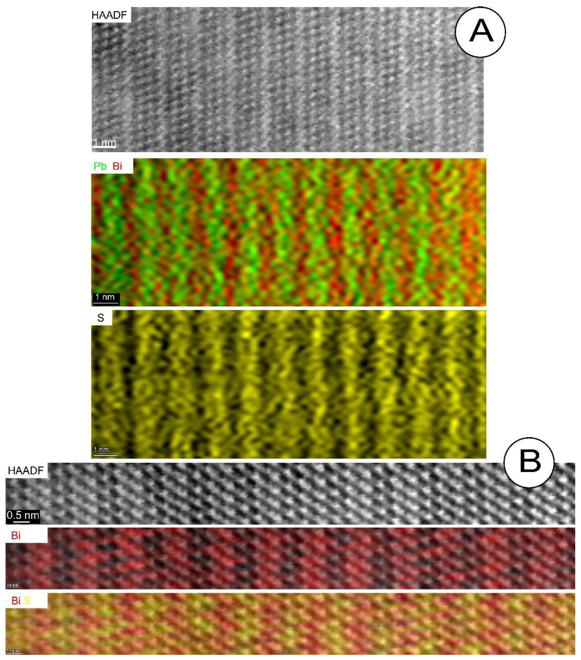
4.3. Nanoscale Characterization

The data presented here for the four chalcogenides derives from one TEM foil for each species, apart from joséite-A for which two foils were prepared (Supplementary Materials, Figures S1 and S2). Laitakarite displays a fine-grained aggregate at the contact with native bismuth (2-µm-wide lamella in the centre of the foil) as well as sub-micron-scale acicular inclusions of galena and bohdanowiczite (Supplementary Materials, Figure S1). Joséite-B was studied from a foil cut across the boundary with adjacent hedleyite (Supplementary Materials, Figure S2). The latter is identified from EPMA data only (see [2]) as the stacking sequences could not be imaged due to grain orientation on [1]. Joséite-A is truncated at the base or on the side by chlorite and native bismuth (Supplementary Materials, Figure S2).
Chemical mapping of laitakarite at the contact with native bismuth shows that Ag and trace Pb is preferentially distributed into the native bismuth (Figure 5A). Tiny inclusions of galena shown on this map become more abundant ~150 nm away from the contact with native bismuth, forming sets of acicular needles of galena and bohdanowiczite (Supplementary Materials, Figure S1). STEM EDS maps of such associations show the presence of nanoscale galena at the margins between bohdanowiczite and host laitakarite (Figure 5B). The presence of detectable sulphur within bohdanowiczite indicates this is probably an intermediate member of the matildite–bohdanowiczite solid solution (AgBiS2–AgBiSe2).

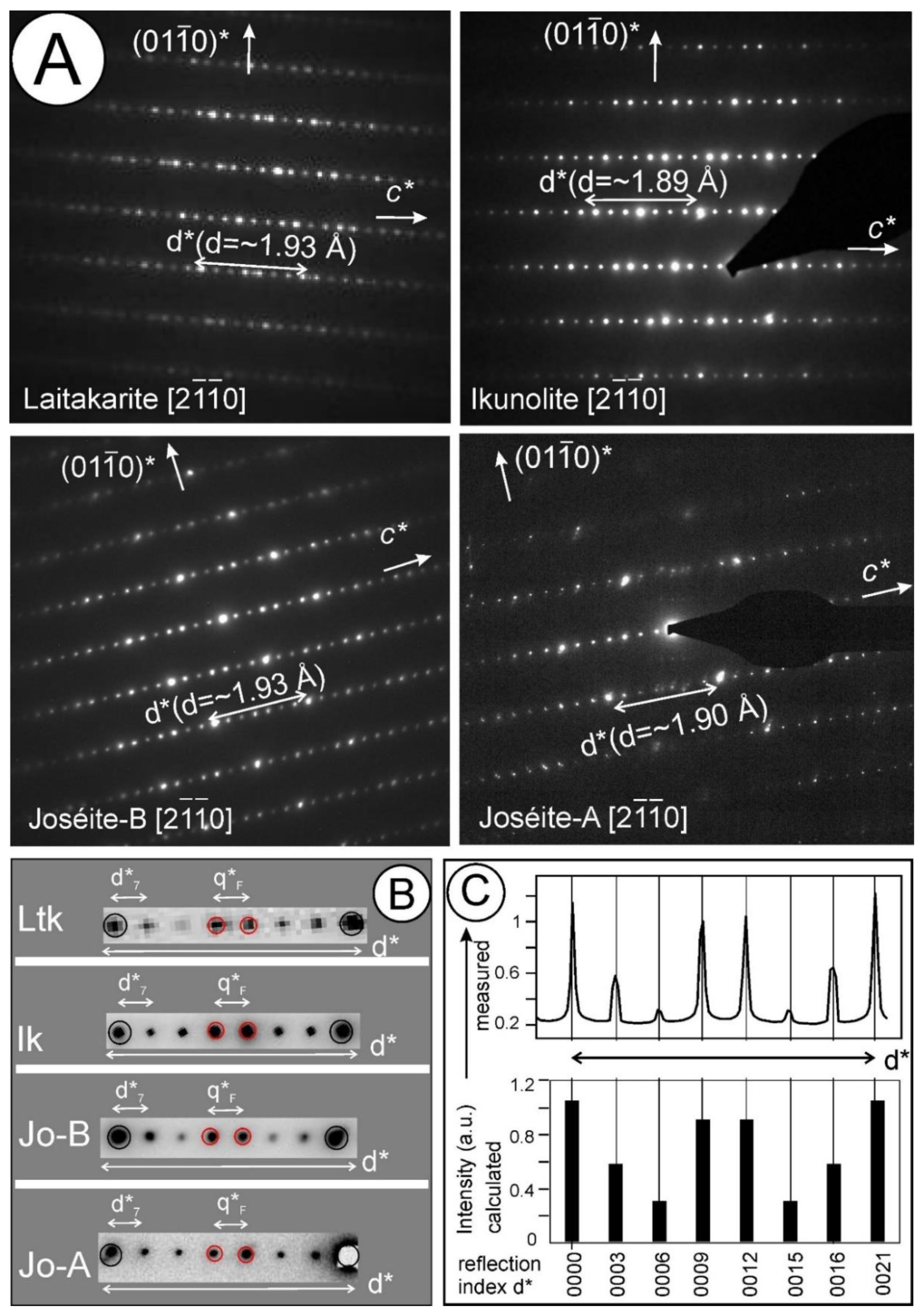
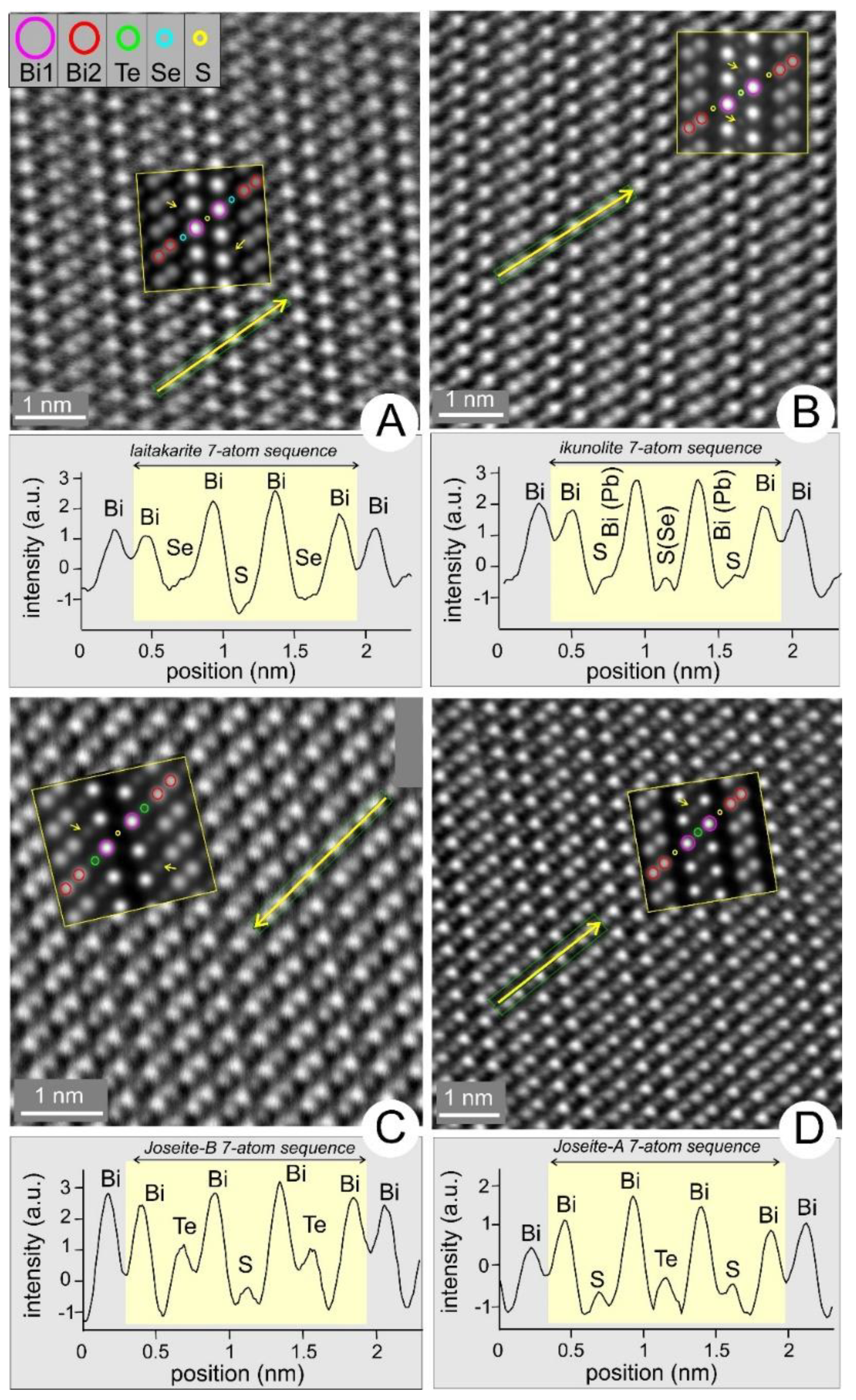
4.3.1. Stacking Sequences in Bi4X3 Phases

All four species show regular stacking sequences with repeats of ~d~1.4 nm, representing the width of the seven-atom layer measured between atom arrays representing the Bi–Bi pairs (see below) (Figure 6A–D). Such regular sequences occur with the same orientation across the length of each species in a given foil, and were imaged by tilting the specimen on a [ 2 1 ¯ 1 ¯ 0 ] zone axis for each species. The high degree of layer-stack ordering is also revealed from the selected area electron diffraction (SAED) patterns obtained from each foil (Figure 7). HAADF STEM images of sequences of up to nine repeats (Figure 6A–D) show the Bi–Bi pairs as closely-spaced double arrays of atoms, of variable intensity from one species to another, e.g., brightest in joséite-B relative to the other species. The interpretation of images is concordant with STEM simulations for each species. The Bi–Bi pairs are difficult to recognize in phases in the present study that show lattice distortion such as laitakarite and joséite-A (Figure 6A,D). This is in sharp contrast with the layer sequences in five-atom layer phases, which are separated by Te–Te pairs with van der Waals bonds, readily recognizable on HAADF STEM images (e.g., [14]). Subtle differences also appear due to the presence of more than a single chalcogen (Se and S in laitakarite, Te and S in joséite-A and -B), as well as the relatively high Pb content of ikunolite. Laitakarite and ikunolite appear broadly similar, in that the central part of the layer stands out relative to the Bi–Bi pairs. STEM simulations (Figure 6A–D) show a good match with the sequences for each of the four species.
The layer sequence in interface-modulated structures can be calculated from electron diffractions using the correlation between the displacement vector (qF*) and the rhombohedral subcell defined by the d* interval (d = 1/d* = ~2 Å) along the c* axis in the tetradymite homologous series ([2,6]; Figure 7). The parameter qF* corresponds to the distance between two brighter satellites in the centre of d* and the layer stack is depicted by the number of divisions (i) within this interval. The smallest distance between any two reflections (dN*) across d* corresponds to the width of a given N layer type (N = number of atoms in the layer) and can be calculated from:
(1)
qF* = i × dN* = (i × d*)/N leading to:
(2)
dN = qF/i and N = (i × qF)/d
The SAED patterns for the four species show a single layer stack (I = 1) with seven divisions across d* (Figure 7A), in this case dN* = qF* and dN = d × N = ~1.4 nm for the seven-atom layer (d = ~2 Å and N = 7). Measurements on the images and corresponding SAED (Figure 6 and Figure 7A) show the d7 width is in the range 1.33–1.35 Å, with corresponding values of d in the range 1.89–1.93 Å. Using c = 3 × d, the calculated c parameter is 40.5 Å for laitakarite and joséite-B, 39.6 Å for ikunolite, and 39.9 Å for joséite-A. These are close to data reported for species from the joséite-B isoseries with comparable compositions to those studied here ([1], and references therein). The four species are typified by the same modulation along the d* interval with reflection intensity concordant with the variation of the sum of intensities for (N – i)/2 reflections calculated by Ciobanu et al. (Table 3 and Figure 9h in [2]) using the fractional shift method (Figure 7B,C).

4.3.2. Identity of Atoms in the Layers

High-resolution imaging of atomic arrangements within the seven-atom layers discussed here are shown in Figure 8. Variation in the intensity of the HAADF signal along the <01 1 ¯ 7> lattice direction shows differences between the Bi atoms in internal and external positions within the layers (Bi1 and Bi2, respectively). The signal profiles show lower intensity for Bi2 relative to Bi1 within each phase but with a greater difference in laitakarite, ikunolite and joséite-A, relative to joséite-B. Such Z-contrast differences are enhanced for species with chalcogens of lower atomic weight, such as S or Se, compared to Te. The inverse distributions of S and Te in joséite-B compared to joséite-A, i.e., Bi2–Te–Bi1–S–Bi1–Te–Bi2, and Bi2–S–Bi1–Te–Bi1–S–Bi2, respectively, are indicated by higher and lower signal intensities across the atom sequences (Figure 8C,D). STEM simulations for the seven-atom sequences in each phase show good correlation with the images and signal variation across the profiles (insets to Figure 8A–D).
The distribution of Pb in ikunolite and S in joséite-A is shown on high-resolution maps of the layer sequences (Figure 9). These show that Pb is associated with the Bi1 position, located centrally in the ikunolite layer (Figure 9A). In joséite-A, the highest Bi concentration overlaps with the Bi2 locations on the margins of the layer, whereas S is highest in the central part (Figure 9B). Sulphur should be placed between the Bi2 and Bi1 positions, flanking the margins of the central Bi1–Te–Bi1 segment of the layer, but this cannot be well discriminated on the maps presented here. The compositions calculated from several maps, including the one in Figure 9B, do however show a close fit to joséite-A stoichiometry, as shown in Table 4.

4.3.3. Nanoscale Inclusions and Lattice-Scale Defects

Inclusions of galena are common throughout the joséite-B specimen (Figure 10). These are observed as sets of thin, 1–2 nm-wide needles, or wider, ~100 nm-thick slivers oriented parallel with the layer stacking in host joséite-B (Figure 10A). Terminations of single needles of galena oriented on the [110] zone axis are accommodated across contacts between two layers of joséite-B (Figure 10B). The narrowest PbS inclusions are imaged as single or double arrays of Pb atoms positioned in the centre of the tellurosulphide (Figure 10C). In detail, the Pb (and adjacent S) atoms along <111> directions in galena can fit either along < 01 1 ¯ 7 > directions in the seven-layer telluride, or alternatively, as twins/kink planes in joséite-B (Figure 10D). A single ‘PbS’ unit inserted within the telluride forms a nine-atom sequence: Bi–Te–Bi–S–[Pb–S]–Bi–Te–Bi, giving the composition PbBi4Te2S2.
In contrast to joséite-B, which has a low Pb content (mean 0.2 wt.%), the species with the highest Pb concentration analysed here, ikunolite (mean 6.7 wt.%), contains no galena inclusions. Ikunolite is nonetheless characterised by numerous defects, which occur as ‘harmonic,’ screw dislocations along < 01 1 ¯ 0 > directions in the Bi–chalcogenide (Figure 11A,B). In detail, the atom displacements lead to dilational swells and kinks between and along the Bi layers (Figure 11B) and these are associated with nucleation of inclusions in laitakarite (Figure 11C,D). As in joséite-B, galena occurs as lamellae that are coherently stacked within the Bi–chalcogenide host, but in this case, as observed in ikunolite, abundant screw dislocations occur (Figure 11C). The kinks along the galena are accommodated by defects whereby splitting and merging of atom arrays are observed, i.e., a Pb array connects with a double Bi–Bi atom array and vice versa (Figure 11D). A comparison can be made with dislocations along 1/3<0111> directions in Bi2Te3 nanowires, which have dissociated components leading to formation of seven-atom layers of the Bi3Te4 type and accounting for changes in chemical composition [32].
In the case discussed here, such lattice-scale defects can also accommodate more complex chemical changes, e.g., enrichment in Pb, Ag, Se, and S, coupled with relative depletion in Bi, leading to the formation of needles containing bohdanowiczite and galena (Figure 12). Galena occurs as single-orientation lamellae whereas bohdanowiczite is polygranular (Figure 13A–C). The Ag–Bi–selenide is identified from images and fast Fourier transform (FFT) patterns of bohdanowiczite tilted on the [ 2 2 ¯ 01 ] zone axis, which is very similar to the adjacent galena tilted on a [110] zone axis (Figure 13D,E).

5. Discussion

5.1. Relationships with Other Phases

Our study shows that phases of the Bi4X3 isoseries [1] represent the Bi2kTe3 (k = 2) module within the tetradymite series [2]. The ED patterns show they all are seven-fold superstructures of a rhombohedral subcell defined by the d* interval (d = 1/d* = ~2 Å) along the c* axis with modulation matching the calculation of reflection intensity using the fractional shift method for Bi4X3 compounds (Figure 7 [2]). In detail, measurements of d* and d7 distances on ED patterns and images (Figure 6 and Figure 7A) do show differences for each of the discussed phases. Although the individual crystal structures could be better refined if using dynamical diffraction refinement or precession electron diffraction to eliminate dynamical effects, e.g., [33,34,35], such dedicated methods were not used for the present study, which is focused on imaging the structures and correlating such imaging with generic homology in the tetradymite series.
Nonetheless, the ED patterns of the four species representing the Bi–X–Bi–X–Bi–X–Bi mixed-layer chalcogenide structure in the tetradymite series [2] will show similarities with those of analogous chalcogen-rich phases with the same number of atoms, i.e., X–Bi–X–Bi–X–Bi–X, such as the seven-atom layer member of the aleksite homologous series [2,13,36]. HAADF STEM imaging and STEM EDX mapping can, however, reveal the internal structure of the layers, confirming published structures in which Bi–Bi pairs are observed at the margins of each seven-atom layer (Figure 6, Figure 7, Figure 8 and Figure 9). In the Bi4X3 isoseries, HAADF STEM imaging reveals the tight Bi2–Bi2 bonding, in agreement with the metallic bonding stipulated from atomic structure determination and band structure calculations for BixSey phases [37].
Species from the Bi4X3 isoseries are therefore distinct from the five-atom layer phases of the Bi2X3 isoseries (tetradymite, tellurobismutite, etc.) which are linked by van der Waal bonds between exterior chalcogen atoms, a feature shared by all homologues of the aleksite series [15,36], e.g., Te–Bi–S–Pb–S–Bi–Te in aleksite (PbBi2Te2S2), the seven-atom member of the series.
It would be most interesting to use HAADF STEM imaging to assess the identity of mineral phases with Bi3X4 stoichiometry, which can be thought of similarly, e.g., Te–Bi–Te–Pb–Te–Bi–Te in rucklidgeite, (Bi,Pb)3Te4, and with expansion to other phases with Bi3X4 stoichiometry. Such species, if they have a simple seven-atom layer sequence, do not obey the homology of the tetradymite series Bi2kX3, and should thus be formed by a combination of five- and seven-atom layers (see [2]). Additionally, such phases also have Pb-rich variants, suggesting a possible link to other series such as the aleksite series [36]. Rucklidgeite was defined as (Bi, Pb)3Te4 [38] but it was later established that the Pb content is variable, up to one a.p.f.u., and probably not essential [39]. Both lead-bearing and lead-free members of a Bi3Te4–PbBi2Te4 solid-solution series are described from several localities (see Figure 15 and extensive referencing in [1]). Cook and Ciobanu [40] documented both low-Pb rucklidgeite (0.02 Pb a.p.f.u.) and Pb-bearing rucklidgeite ((Pb0.82–0.87Bi2.11–2.16)S3(Te,Se,S)4) in the same ore system. The same may apply to poubaite, PbBi2(Se,Te,S)4 [41,42], a less common mineral. Cook et al. [1] raised the possibility of additional phases with a rucklidgeite-like stoichiometry based on published data for unnamed Bi3(Te,S)4 [38,43,44,45] and for a phase with the empirical composition Bi3(Te1.67–2.21Se0.67–1.65S0.70–1.14)4 [46].

5.2. Mixed Sites versus Inclusions: The Role and Location of Lead

Unlike other species in the tetradymite homologous series, all Bi4X3 phases often, although not ubiquitously, contain several wt.% Pb [1]. Here we show that Pb can be incorporated into the crystal structure but can also form nanoscale inclusions of galena (Figure 9, Figure 10, Figure 11 and Figure 12). Incorporation of Pb within a mixed site with Bi1 is inferred from the mapping of ikunolite, the species with highest Pb content analysed here (~0.3 a.p.f.u.). In contrast to the metal (cation) sites, the present data show very little tendency among chalcogens towards mixed site occupancy (Table 2, Table 3 and Table 4).
Although ikunolite also hosts the greatest concentration of other cations, particularly measurable Ag (~0.005 a.p.f.u.), the sum of other monovalent cations (including Ag and Au) is much lower than that required for charge balance compensation considering the substitution Pb2+ + M+ = Bi3+. A comparable problem occurs with presence of structural Pb within members of the Bi3X4 isoseries, as introduced above. Based on the absence of nanoscale inclusions in the material analysed here, we are confident that the Pb measured in ikunolite is structurally bound.
Interestingly, five of the nine microprobe analyses that contain measurable Au (in the range 700–2290 ppm Au) were obtained from the location of the investigated foil. There is no direct correlation between Au and Ag concentrations, even though their sum is 0.014 a.p.f.u (0.006 a.p.f.u. Au and 0.008 a.p.f.u. Ag)—relatively high but still an order of magnitude below Pb measured in the same analyses (~0.3 a.p.f.u.). This implies no direct correlation between the presence of ‘exotic’ precious trace elements and Pb, at least not in the present data. Nonetheless, the EPMA measurements confirm measurable Au in ikunolite from Ashio at levels comparable with those reported from laser-ablation inductively coupled mass spectrometry [29]. If validated by other methods of atomic structural determination, the presence of heterovalent mixed cation sites in Bi–chalcogenides is also important for structural incorporation of Ag and Au, particularly in high-grade Au ores [14].
Galena occurs as nanoscale inclusions in both laitakarite and joséite-B (~0.14 and 0.01 a.p.f.u., respectively). This is despite the fact that ikunolite and laitakarite show widespread lattice-scale defects whereas joséite-B lacks such defects (Figure 10 and Figure 11). We suggest that Pb behaviour is controlled by the local environment, e.g., ikunolite formation is buffered by high-Pb since it co-exists with, and also contains, ubiquitous inclusions of a Pb–Bi sulphosalt from the lillianite–gustavite solid solution (Figure 2C,D). The abundant lattice-scale defects in ikunolite and laitakarite can be attributed to strain-induced deformation, either during vein re-opening at Ashio [47] or superimposed metamorphism at Orijärvi [48].
The formation of single and double PbS units through the centre of seven-atom layers in joséite-B (Figure 10) suggests the possibility of an additional homologous series starting from joséite-B and extending to PbBi4Te2S2 (nine-atom layer), Pb2Bi4Te2S4 (eleven-atom layer) and so on, in a manner comparable the aleksite series ([15,36]; see above).

6. Conclusions and Implications

The direct visualisation of structures by HAADF STEM and nanoscale chemical mapping of layer sequences unequivocally confirms the identity of the Bi4S3–Bi4Se3–Bi4Te3 isoseries. Laitakarite, ikunolite, joséite-B, and joséite-A are mixed-layer structures representing the Bi2kTe3 (k = 2) module within the tetradymite series. SAED patterns confirm they are seven-fold superstructures of a rhombohedral subcell with c/3 = d~1.89–1.93 Å. Modulation along the d* interval matches calculations of reflection intensity using the fractional shift method for Bi4X3. The internal structure in each species can be discerned by high-resolution imaging. We confirm the presence of mixed sites for cations, particularly Pb. The role of Pb is important in understanding the incorporation of Ag and Au in Bi–chalcogenides, as well as the formation of other, parallel homologous series of Pb–Bi–chalcogenides, including those from the aleksite series. HAADF STEM imaging of crystal structures will continue to play a valuable role in understanding relationships between phases in the tetradymite series and for the characterization of potential additional members.

Supplementary Materials

The following are available online at https://www.mdpi.com/article/10.3390/min11090920/s1, Table S1: EPMA setup for analysis, Table S2: Interference corrections, Table S3: Standard information, Figure S1: Secondary electron and HAADF STEM images showing aspects of the laitakarite foil, Figure S2: HAADF STEM images showing aspects of the four studied foils.

Author Contributions

N.J.C. and C.L.C. designed the research and wrote the paper. A.D.S. provided assistance with the operation of the Titan Themis S/TEM microscope and data acquisition/processing. B.P.W. provided assistance with EPMA data acquisition/processing. K.E. provided advice and guidance throughout. All authors participated in editing the manuscript. All authors have read and agreed to the published version of the manuscript.

Funding

This work was funded by The University of Adelaide as a Women’s Research Excellence Award to C.L.C.

Data Availability Statement

Full data are available from the authors upon request.

Acknowledgments

Specimens were kindly made available to the authors by Krister Sundblad (laitakarite), Maasaki Shimizu (ikunolite) and Bill Howard (joséite-A and -B). Three anonymous reviewers are thanked for their valuable comments.

Conflicts of Interest

The authors declare no conflict of interest..

References

  1. Cook, N.J.; Ciobanu, C.L.; Wagner, T.; Stanley, C.J. Minerals of the system Bi-Te-Se-S related to the tetradymite archetype: Review of classification and compositional variation. Can. Miner. 2007, 45, 665–708. [Google Scholar] [CrossRef]
  2. Ciobanu, C.L.; Pring, A.; Cook, N.J.; Self, P.; Jefferson, D.; Dima, G.I.; Melnikov, V. Chemical-structural modularity in the tetradymite group: A HRTEM study. Am. Miner. 2009, 94, 517–534. [Google Scholar] [CrossRef]
  3. Van Landuyt, J.; De Ridder, R.; Gevers, R.; Amelinckx, S. Diffraction effects due to shear structures: A new method for determining the shear vector. Mater. Res. Bull. 1970, 5, 353–362. [Google Scholar] [CrossRef]
  4. Imamov, P.M.; Semiletov, S.A. The crystal structure of the phases in the system Bi-Se, Bi-Te, and Sb-Te. Sov. Phys. Crystallogr. 1971, 15, 845–850. [Google Scholar]
  5. Van Tendeloo, G.; van Dyck, D.; Kuypers, S.; Amelinckx, S. Electron diffraction effects in mixed layer compounds. I. Theorteical considerations. Phys. Stat. Sol. 1989, 101, 339–354. [Google Scholar] [CrossRef]
  6. Frangis, N.; Kuypers, S.; Manolikas, C.; Van Tendeloo, G.; Amelinckx, S. Continuous series of one-dimensional structures in compounds based on M2X3 (M = Sb, Bi, X = Se, Te). J. Solid State Chem. 1990, 84, 314–334. [Google Scholar] [CrossRef]
  7. Shelimova, L.E.; Karpinsky, O.G.; Kosyakov, V.I.; Shestakov, V.A.; Zemskov, V.S.; Kuznetsov, F.A. Homologous series of layered tetradymite-like compounds in Bi-Te and GeTe-Bi2Te3 systems. J. Struct. Chem. 2000, 41, 81–87. [Google Scholar] [CrossRef]
  8. Lind, H.; Lidin, S. A general structure model for Bi-Se phases using a superspace formalism. Solid State Sci. 2003, 5, 47–57. [Google Scholar] [CrossRef]
  9. Heremans, J.P.; Cava, R.J.; Samarth, N. Tetradymites as thermoelectrics and topological insulators. Nat. Rev. Mater. 2017, 2, 17049. [Google Scholar] [CrossRef]
  10. Manzano, C.V.; Martin-Gonzalez, M. Electrodeposition of V-VI Nanowires and Their Thermoelectric Properties. Front. Chem. 2019, 7, 516. [Google Scholar] [CrossRef]
  11. Bos, J.-W.G.; Faucheux, F.; Downie, R.A.; Marcinkova, A. Phase stability, structures and properties of the (Bi2)m (Bi2Te3)n natural superlattices. J. Solid State Chem. 2012, 193, 13–18. [Google Scholar] [CrossRef] [Green Version]
  12. Kuznetsov, P.I.; Yapaskurt, V.O.; Shchamkhalova, B.S.; Shcherbakov, V.D.; Yakushcheva, G.G.; Luzanaov, V.A.; Jitov, V.A. Growth of Bi2Te3 films and other phases of the Bi-Te system by MOVPE. J. Cryst. Growth 2016, 455, 122–128. [Google Scholar] [CrossRef]
  13. Mao, C.; Tan, M.; Zhang, L.; Wu, D.; Bai, W.; Liu, L. Experimental reinvestigation and thermodynamic description of Bi-Te binary system. Calphad 2018, 60, 81–89. [Google Scholar] [CrossRef]
  14. Ciobanu, C.L.; Birch, W.D.; Cook, N.J.; Pring, A.; Grundler, P.V. Petrogenetic significance of Au–Bi–Te–S associations: The example of Maldon, Central Victorian gold province, Australia. Lithos 2010, 116, 1–17. [Google Scholar] [CrossRef]
  15. Cook, N.J.; Ciobanu, C.L.; Liu, W.Y.; Slattery, A.; Wade, B.P.; Mills, S.; Stanley, C.J. Polytypism and polysomatism in mixed-layer chalcogenides: Characterization of PbBi4Te4S3 and inferences for ordered phases in the aleksite series. Minerals 2019, 9, 628. [Google Scholar] [CrossRef] [Green Version]
  16. Cook, N.J.; Ciobanu, C.L.; Ehrig, K.; Slattery, A.; Verdugo-Ihl, M.R.; Courtney-Davies, L.; Gao, W. Advances and Opportunities in Ore Mineralogy. Minerals 2017, 7, 233. [Google Scholar] [CrossRef] [Green Version]
  17. Ciobanu, C.L.; Kontonikas-Charos, A.; Slattery, A.; Cook, N.J.; Wade, B.P.; Ehrig, K. Short-range stacking disorder in mixed-layer compounds: A HAADF STEM study of bastnäsite-parisite intergrowths. Minerals 2017, 7, 227. [Google Scholar] [CrossRef] [Green Version]
  18. Medlin, D.L.; Yang, N.; Spataru, C.D.; Hale, L.M.; Mishin, Y. Unraveling the dislocation core structure at a van der Waals gap in bismuth telluride. Nat. Commun. 2019, 10, 1820. [Google Scholar] [CrossRef] [Green Version]
  19. Medlin, D.L.; Snyder, G.J. Atomic-scale interfacial structure in rock salt and tetradymite chalcogenide thermoelectric materials. JOM 2013, 65, 390–400. [Google Scholar] [CrossRef]
  20. Ciobanu, C.L.; Cook, N.J.; Maunders, C.; Wade, B.P.; Ehrig, K. Focused Ion Beam and Advanced Electron Microscopy for Minerals: Insights and Outlook from Bismuth Sulphosalts. Minerals 2016, 6, 112. [Google Scholar] [CrossRef] [Green Version]
  21. Li, W.; Ciobanu, C.L.; Slattery, A.; Cook, N.J.; Liu, W.; Wade, B.P.; Xie, D.Q. Chessboard structures: Atom-scale imaging of homologues from the kobellite series. Am. Miner. 2019, 104, 459–462. [Google Scholar] [CrossRef]
  22. Vorma, A. Laitakarite, a new Bi–Se-mineral. Bull. Comm. Géol. Finl. 1960, 188, 1–10. [Google Scholar]
  23. Yamana, K.; Kihara, K.; Matsumoto, T. Bismuth tellurides: BiTe and Bi4Te3. Acta Cryst. 1979, B35, 147–149. [Google Scholar] [CrossRef] [Green Version]
  24. Stasova, M.M. The crystal structure of bismuthum selenide Bi4Se3. Izv. Akad. Nauk SSSR 1968, 4, 28–31. [Google Scholar]
  25. Kato, A. Ikunolite, a new bismuth mineral from the Ikuno mine, Japan. Miner. J. 1959, 2, 397–407. [Google Scholar] [CrossRef] [Green Version]
  26. Armstrong, J.T. Quantitative analysis of silicate and oxide minerals: Comparison of Monte Carlo, ZAF, and φ(ρz) procedures. In Microbeam Analysis; Newbury, D.E., Ed.; San Francisco Press: San Francisco, CA, USA, 1988; pp. 239–246. [Google Scholar]
  27. Donovan, J.J.; Rowe, M. Techniques for Improving Quantitative Analysis of Mineral Glasses. Geochim. Cosmochim. Acta 2005, 69 (Suppl. 1), A589, (Goldschmidt Conference Abstracts 2005). [Google Scholar]
  28. Ciobanu, C.L.; Cook, N.J.; Pring, A.; Green, L. Focussed ion beam—Transmission electron microscopy applications in ore mineralogy: Bridging micron- and nanoscale observations. Ore Geol. Rev. 2011, 42, 6–31. [Google Scholar] [CrossRef]
  29. Ciobanu, C.L.; Cook, N.J.; Pring, A.; Brugger, J.; Danyushevsky, L.V.; Shimizu, M. ‘Invisible gold’ in bismuth chalcogenides. Geochim. Cosmochim. Acta 2009, 73, 1970–1999. [Google Scholar] [CrossRef]
  30. Ciobanu, C.L.; Cook, N.J.; Sundblad, K. Genetic insights from exotic trace mineral associations at Orijärvi and Iilijärvi, S.W. Finland. In Metallogeny of Precambrian Shields, Ky’iv, Ukraine; Symposium Abstract Volume: Geological Survey: Ky’iv, Ukraine, 2002; p. 5. [Google Scholar]
  31. Ciobanu, C.L.; Slattery, A.; Cook, N.J.; Wade, B.P.; Ehrig, K. Bi8Te3, the 11-atom layer member of the tetradymite homologous series. Minerals. in review.
  32. Medlin, D.; Erickson, K.; Limmer, S.; Yelton, W.; Siegal, M.P. Dissociated 1/3 dislocations in Bi2Te3 and their relationship to seven-layer Bi3Te4 defects. J. Mater. Sci. 2014, 49, 3970–3979. [Google Scholar] [CrossRef]
  33. Dudka, A.P.; Avilov, A.S.; Lepeshov, G.G. Crystal structure refinement from electron diffraction data. Crystallogr. Rep. 2008, 53, 530–536. [Google Scholar] [CrossRef]
  34. Palatinus, L.; Petricek, V.; Corrêa, C.A. Structure refinement using precession electron diffraction tomography and dynamical diffraction: Theory and implementation. Acta Cryst. 2015, A71, 235–244. [Google Scholar] [CrossRef]
  35. Hoser, A.A.; Madsen, A.Ø. Dynamic quantum crystallography: Lattice-dfynamical models refined against diffraction data. I. Theory. Acta Cryst. 2016, A72, 206–214. [Google Scholar] [CrossRef]
  36. Cook, N.J.; Ciobanu, C.L.; Stanley, C.J.; Paar, W.; Sundblad, K. Compositional data for Bi-Pb tellurosulfides. Can. Miner. 2007, 45, 417–435. [Google Scholar] [CrossRef]
  37. Gaudin, E.; Jobic, S.; Evain, M.; Brec, R.; Rouxel, J. Charge balance in some BixSey phases through atomic structure determination and band structure calculations. Mater. Res. Bull. 1995, 30, 549–561. [Google Scholar] [CrossRef]
  38. Zav’yalov, Y.N.; Begizov, V.D.; Stepanov, V.I. Redetermination of wehrlite and the first find of tsumoite in the USSR. Zap. Vses. Miner. Obshchest. 1978, 107, 544–553. (In Russian) [Google Scholar]
  39. Kase, K.; Kusachi, I.; Kishi, S. Rucklidgeite solid solution in the Yanahara deposit, Japan. Can. Miner. 1993, 31, 99–104. [Google Scholar]
  40. Cook, N.J.; Ciobanu, C.L. Bismuth tellurides and sulphosalts from the Larga hydrothermal system, Metaliferi Mts., Romania: Paragenesis and genetic significance. Miner. Mag. 2004, 68, 301–321. [Google Scholar] [CrossRef] [Green Version]
  41. Čech, F.; Vavřín, I. Poubaite, PbBi2(Se,Te,S)4, a new mineral. N. Jb. Miner. Monatsh. 1978, 9–19. [Google Scholar]
  42. Shikazono, N.; Nakata, M.; Shimizu, M. Geochemical, mineralogic and geological characteristics of Se- and Te-bearing epithermal gold deposits in Japan. Min. Geol. 1990, 40, 337–352. [Google Scholar]
  43. Kojonen, K.; Johanson, B.; Sipilä, E. The Kiimala gold deposit in Haapavesi, western Finland. Geol. Surv. Finl. Spec. Pap. 1991, 12, 75–79. [Google Scholar]
  44. Spiridonov, E.M. Mineralogy of the metamorphosed plutonogenic gold–quartz Kochar deposit, South Urals. 1. Gold–telluride ores. Zap. Vses. Mine. Obshch. 1995, 124, 24–39. (in Russian). [Google Scholar]
  45. Moloshag, V.P.; Grabezhev, A.I.; Gulyaeva, T.Y. Conditions of formation of tellurides in massive sulfide ores and copper–gold porphyry deposits of the Urals. Zap. Vser. Miner. Obshch. 2002, 131, 40–53. (In Russian) [Google Scholar]
  46. Shimizu, M.; Schmidt, S.T.; Stanley, C.J.; Tsunoda, K. Kawazulite and unnamed Bi3(Te,Se,S)4 in Ag–Bi–Te–Se–S mineralization from the Suttsu mine, Hokkaido, Japan. N. Jb. Miner. Abh. 1995, 169, 305–308. [Google Scholar]
  47. Geological Survey of Japan Mines. Summary Reports. Vol. 1, North-East Japan and Vol. 2, South-West Japan; Report 260; Geological Survey of Japan: Tsukuba, Japan, 1980; Appendices 1 (310 pp.) and 2 (266 pp.). [Google Scholar]
  48. Schruers, J.; Westra, L. Cordierite-orthopyroxene rocks: The granulite facies equivalents of the Orijärvi cordierite-anthophyllite rocks in West Uusimaa, southwest Finland. Lithos 1985, 18, 215–228. [Google Scholar] [CrossRef]
Figure 1. Ball-and-stick (A) and space filling (B) crystal models for pilsenite, laitakarite, and ikunolite viewed along the a axis. The three minerals are isostructural with slightly modified a and c dimensions. The two structural positions for Bi and chalcogen (X = Te, Se, S) are schematically marked at the top. Structures constructed in CrystalMaker® (v10.5.7) using .cif files based on Yamana et al. [23] for pilsenite (Bi4Te3), Stasova [24] for laitakarite (Bi4Se3), and Kato [25] for ikunolite (Bi4S3).
Minerals 11 00920 g001
Figure 2. BSE images (except C and E, which are reflected light photomicrographs) showing petrographic aspects of studied specimens. (A) Platy laitakarite (Ltk) with location of FIB-cut indicated (black diamond-shaped area). (B) Detail of area from which the foil was extracted prior to cross-sectioning. This shows typical inclusions of native bismuth (Bi) and minor bohdanowiczite (Boh) within laitakarite. White arrows show sub-micron-scale sets of acicular inclusions identified in the nanoscale study as galena + bohdanowiczite. (C) Ikunolite (Iku) as coarse laths within native bismuth. (D) Detail showing inclusions of lillianite–gustavite solid solution (Lil) within ikunolite. Location of FIB-cut is indicated by white circle. (E) Hedenbergite (Hbg) skarn specimen from Hedley, containing disseminations of Bi-minerals (e.g., marked by white circle). Abundant quartz (Qz) is also present. (F) Multi-component Bi-mineral assemblage from the circle marked in (E) associated with scheelite (Sch). (G) Detail of Bi-mineral assemblage in (F) comprising joséite-B (JoB), native bismuth, hedleyite (Hed) and unnamed Bi8Te3. Yellow bar shows location of FIB-cut. (H) Small grains of joséite-A (marked by white boxes) along trails with retrograde chlorite (replacing hedenbergite).
Minerals 11 00920 g002
Figure 3. BSE images (A,B) and secondary electron images (C,D) showing the two joséite-A grains cut across (yellow lines show the FIB cuts) for TEM foils. Cross-section imaging of the two grains (C,D) showing the extension of the grains at depth. Note small size and intense fracturing of the tellurides.
Minerals 11 00920 g003
Figure 4. Representation of compositional data for Bi4X3 phases. (A) Bi4S3- Bi4Se3–Bi4Te3 ternary diagram. (B) Plot of Pb/total metals vs. Te/(Te+Se+S). Iku–ikunolite, Lait–laitakarite, Jo-A–joséite-A, Jo-B–joséite-B.
Minerals 11 00920 g004
Figure 5. (A) STEM EDS element maps showing laitakarite (Ltk) adjacent to native bismuth, and (B) sets of acicular inclusions with galena (Gn) and bohdanowiczite (Boh), also arrowed in (A).
Minerals 11 00920 g005
Figure 6. HAADF STEM images and respective STEM simulations (below each image) in (AD) showing ordered stacking sequences on the [ 2 1 ¯ 1 ¯ 0 ] zone axis of each of the four analysed phases as labelled: laitakarite (Ltk) in (A), ikunolite (Ik) in (B), joséite-B (Jo-B) in (C), and joséite-A (Jo-A) in (D). The double Bi–Bi pairs that separate the layers are marked by yellow lines on both images and simulations. Note that the Bi–Bi pairs are closely spaced. The images were obtained using drift-corrected frame integration (DCFI) procedures and application of filters to eliminate noise.
Minerals 11 00920 g006
Figure 7. (A) Selected area electron diffraction (SAED) on the [ 2 1 ¯ 1 ¯ 0 ] zone axis for each of the species shown in Figure 6. Note the slight variation in measured d values (d = 1/d*) in the range 1.89–1.93 Å. (B) Details on the reflection distribution and intensity variation along the interval d* obtained from each SAED in (A). Note d*7 = q*F in all four species. (C) Plots showing the match between variation in reflection intensity along d* for ikunolite (upper part) and calculated values for the sum of intensities for the seven-atom layer obtained from [2] (lower part). Indexing along the x axis with respect to the seven-atom-layer superstructure.
Minerals 11 00920 g007
Figure 8. High-resolution HAADF STEM images (obtained by DCFI procedures and filtered to eliminate noise) and intensity profiles (below each image) for ikunolite (A), laitakarite (B), joséite-B (C), and joséite-A (D). Yellow arrows show the location and direction of the HAADF intensity profiles. Insets outlined in yellow are STEM simulations showing the distribution and speciation of the seven-atoms across a single layer. The simulations were obtained using the atomic coordinates for structures (.cif files for the end-member tellurides shown in Figure 1) but with compositional modifications for cation mixed sites/chalcogen speciation within the seven-atom sequence according to EPMA data. Chalcogens that are visible on the STEM simulations are marked by short arrows. Note variation in signal intensity for Bi positions, whereby the Bi–Bi pairs (Bi2 position) have a lower intensity than the two ‘internal’ Bi atoms (Bi1) that alternate with chalcogens and which are better separated on the images. This effect is attenuated on the images/profile for joséite-B more than in the STEM simulation.
Minerals 11 00920 g008
Figure 9. High-resolution STEM EDS element maps for (A) ikunolite and (B) joséite-A. The maps for ikunolite clearly show that Pb is located in the central parts of the layers and not substituted into the Bi–Bi pairs. The maps for joséite-A show the strongest Bi concentration overlaps with the marginal Bi2–Bi2 pairs, whereas S overlaps with the central part of the layers corresponding to a [Bi2–S–Bi1–Te–Bi1–S–Bi2] position topology. Although these element maps do not fully define the location of S between Bi2 and Bi1 atoms, the composition obtained from an integrated spectrum across the mapped area (Table 4) fits joséite-A stoichiometry closely.
Minerals 11 00920 g009
Figure 10. HAADF STEM images showing nanoscale inclusions of galena (Gn) within joséite-B (Jo-B). (A) Sets of parallel galena units (arrowed) in the vicinity of a larger galena inclusion. (B) Termination of a galena strip (5-PbS units) against two sequences of seven-atom layers in joséite-B. (C) Single and double Pb arrays (arrowed) inserted within the centre of a seven-atom layer of joséite-B. (D) Detail of layer intergrowths in (C) with atom overlay showing how the PbS[110] units are incorporated within the existing seven-atom sequence.
Minerals 11 00920 g010
Figure 11. HAADF STEM images (obtained by DCFI procedure and filtered to eliminate noise) of (A,B) ikunolite (Ik) and (C,D) laitakarite (Ltk), showing lattice-scale defects. (A) Field of harmonic screw dislocations along < 01 1 ¯ 0 > directions in ikunolite. (B) Detail of (A) showing dilational swells and jogs (arrowed) along the same layers, implying screw rotation along the direction of the dislocation. (C) Screw and kink dislocations in laitakarite hosting a lamella of galena. (D) Detail of kink defect in galena from (C) showing the dislocations of atom arrays viewed on the [ 2 1 ¯ 1 ¯ 0 ] plane in laitakarite.
Minerals 11 00920 g011
Figure 12. STEM EDS element maps showing an acicular inclusion comprising bohdanowiczite (Boh) between two needles of galena (Gn).
Minerals 11 00920 g012
Figure 13. (A–C) HAADF STEM images and FFT patterns of galena (Gn) and bohdanowiczite (Boh) within laitakarite (Ltk), occurring along the composite inclusion shown on the maps in Figure 11. These are imaged on zone axes as marked on the FFT patterns. (D,E) crop of images in (B,C) and crystal models of the two phases. Overlays (dashed white lines) on the FFT patterns, images, and models highlight the rhombus motif which is common to both species for the respective zone axes.
Minerals 11 00920 g013
Table 1. Specimens studied in this contribution.
MineralSpecimenEmpirical Formula
LaitakariteOrijärvi, Finland(Bi3.93Pb0.14)4.07(Se1.84S1.09)2.93
IkunoliteAshio, Japan(Bi3.67Pb0.30)3.99(S2.99Se0.02)3.01
Joséite-AHedley, B.C., CanadaBi3.98(Te0.85Se0.01S2.17)3.02
Joséite-B(Bi4.08Pb0.01Sb0.01)4.10(Te1.89S1.01)3.90
Background data on these samples was given in Ciobanu et al. [29], and for the laitakarite sample, also in Ciobanu et al. [30].
Table 2. Electron probe microanalysis data for laitakarite (wt.%).
Mean (n = 10)S.D.MinimumMaximum
Pb2.850.122.593.01
Bi80.280.7479.2081.47
S3.430.063.323.49
Se14.180.3013.8414.93
Te<mdl0.010.000.04
Total100.740.8199.30102.01
Pb0.1410.0060.1280.148
Bi3.9280.0243.8783.953
Sum Me4.0690.0224.0184.090
S1.0940.0171.0541.115
Se1.8360.0341.8121.928
Te----
Sum S + Se + Te2.9310.0222.9102.982
Table 3. Electron probe microanalysis data for ikunolite (wt.%).
Mean (n = 41) *S.D.MinimumMaximumMean Au-Bearing
(n = 9) **
Au<mdl0.06<mdl0.230.13
Zn<mdl0.01<mdl0.050.01
Cu<mdl0.02<mdl0.080.01
Ag0.060.06<mdl0.220.09
Fe<mdl0.01<mdl0.03<mdl
Cd0.040.04<mdl0.110.03
Pb6.730.116.547.126.76
Mn<mdl0.01<mdl0.03<mdl
As0.010.03<mdl0.090.02
Sb0.040.03<mdl0.080.02
Bi83.790.3783.0384.5083.96
S10.460.1010.2010.6310.45
Te<mdl0.00<mdl<mdl<mdl
Se0.200.050.120.300.23
Total101.340.37100.53101.97101.71
Calculated formula (7 atom basis)
Au0.0010.003-0.0110.006
Zn0.0010.002-0.0060.001
Cu0.0010.002-0.0120.001
Ag0.0050.005-0.0180.008
Pb0.2970.0050.2890.3170.298
Fe0.0000.001-0.0050.000
Mn0.0000.001-0.0050.000
Cd0.0030.003-0.0090.003
Bi3.6740.0223.6413.7333.673
As0.0010.003-0.0100.002
Sb0.0030.002-0.0060.002
Sum Me3.9870.0193.9514.0303.993
S2.9900.0212.9493.0292.980
Te----0.000
Se0.0240.0060.0140.0350.027
Sum S + Se + Te3.0130.0192.9703.0493.007
mdl: minimum limit of detection; * all data; ** sub-set of analyses above mdl for Au.
Table 4. Electron probe microanalysis data for joséite-B and STEM EDS data for joséite-A (wt.%).
Joséite-B (Bi4Te2S) (n = 20)Joséite-A (Bi4TeS2) (n = 7)
MeanS.D.MinimumMaximumRepresentativeMeanS.D.MinimumMaximum
Pb0.200.080.000.36-----
Bi76.570.4575.5877.2182.3181.770.4281.0782.31
Sb0.070.06<mdl0.16- -- - -
Te21.610.3720.9422.1910.7310.960.3010.6711.42
Se<mdl---0.080.15 0.10 0.03 0.27
S2.910.092.773.096.887.120.226.887.52
Total101.360.44100.10101.95100.00100.00---
Formula on basis of 7 atomsFormula on basis of 7 atoms
Pb0.010.000.000.020.00----
Bi4.080.024.044.133.983.910.053.843.98
Sb0.010.010.000.010.0000.000.000.000.00
Sum Me4.100.024.074.143.983.910.053.843.98
Te1.890.031.821.930.850.860.020.820.89
Se----0.0100.020.010.000.03
S1.010.030.971.072.1662.220.052.172.31
Sum Te + Se + S2.900.022.862.933.023.090.053.023.16
Publisher’s Note: MDPI stays neutral with regard to jurisdictional claims in published maps and institutional affiliations.

