
Straight to Low-Sinuosity Drainage Systems in a Variscan-Type Orogen—Constraints from Tectonics, Lithology and Climate


Abstract
1. Introduction
- What is the impact of the different types of structural geology on the fluvial systems?
- What is the impact of the varied bedrock lithologies on the hydrography and the hydrodynamic evolution?
- What is the impact of Neogene-Quaternary climate on the drainage systems?
- To what extent can the GMS gravel (granulometry-morphology-situmetry) analysis contribute to the hydrodynamics of coarse-grained fluvial deposits?
- Is the elaborated genetic model of the fluvial drainage system applicable to all landform systems in orogenic realms or geodynamically restricted to a special state of crustal maturity?
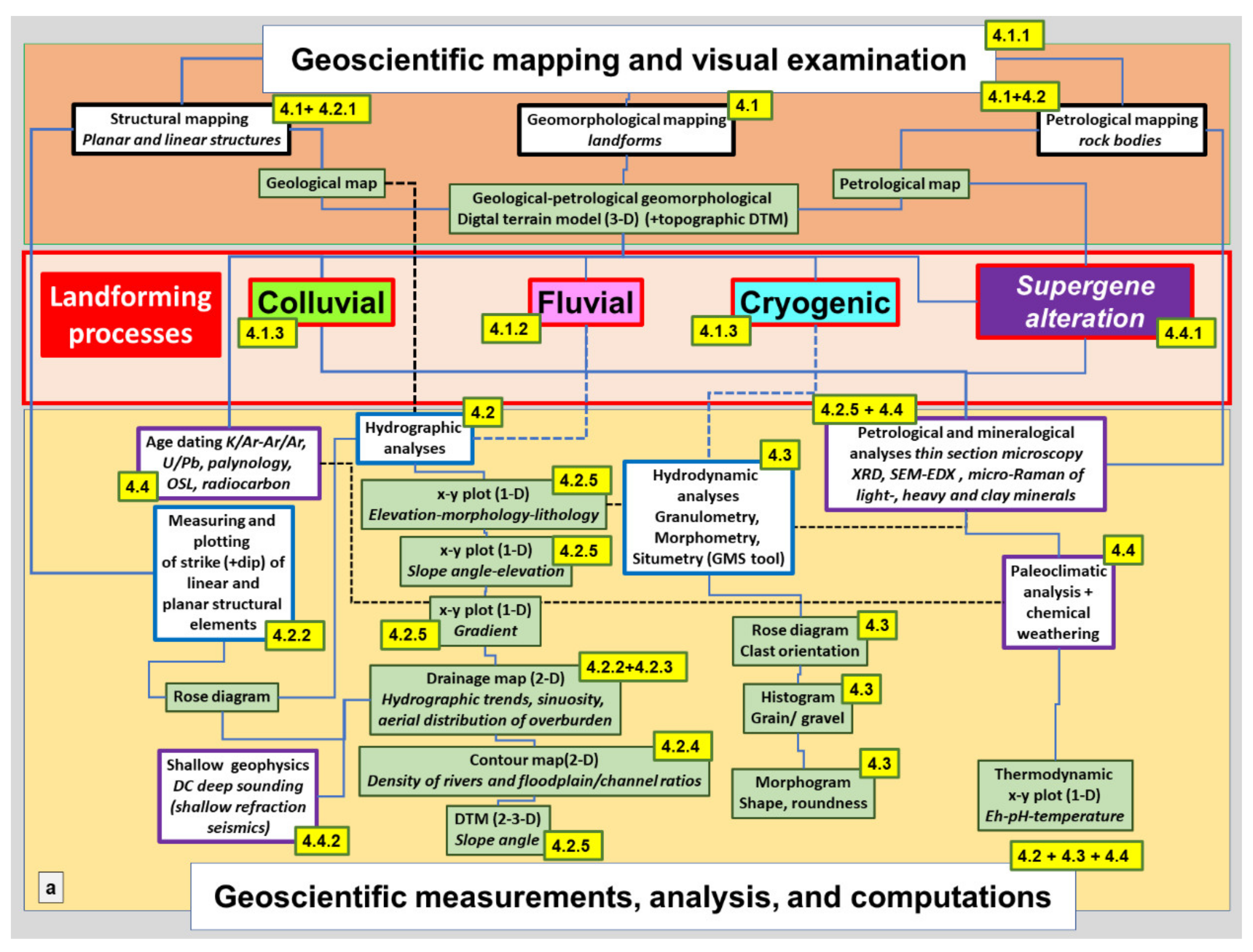
2. Methodology—A Holistic-Modular Approach to Study the Straight to Low Sinuosity Drainage Systems (SSS)
2.1. Strategy of the Flow Chart
2.2. Geoscientific Mapping and Visual Examination
2.3. Geoscientific Analysis, Measurements, and Computations
2.3.1. Laboratory Methods
2.3.2. Field and Desk(top) Methods

| Chanel System | Geological-Geotectonic Setting | Sinuosity Max | Sinuosity Min | Type of Drainage System vs. Structural Setting | Bedrock Lithology |
|---|---|---|---|---|---|
| Very strongly meandering | Foreland basin, basin-and-swell geomorphology (“washboard landscape”) with local volcanic structures | >5 (in the test area mean 8.2916) | 5 | Dip-, anti-dip and strike-stream, in places, with sedimentary trap sites | Sandstone, arkose, limestone, marl, claystone, evaporite (bedded), volcaniclastic and volcanic rocks (non-metamorphosed rocks) See very-low and low-grade metamorphic rocks and felsic intrusive rocks |
| Strongly meandering | 5 (in the test area mean 4.6159) | 2 | Mainly dip, anti-dip stream | ||
| Moderately meandering | Foreland basin, basin-and-swell geomorphology (“washboard landscape”) with local volcanic structures Also, in front of the basement and the basement, proper, (rarely intermediate sediment trap, deposition and catchment areas) | 2 (in the test area mean 1.7209) | 1.5 | Mainly strike-stream | |
| Sinuous (high-sinuosity) | Basement, folded-and faulted ridge- and-reef geomorphology with domal structures | 1.5 (in the test area mean 1.3789) | 1.3 | Dip-, anti-dip and strike-stream in the catchment area (CA) of rivers | (Two)-mica gneiss, mafic gneiss, orthogneiss, metaultrabasic and -basic igneous rocks (medium to high grade metamorphic) |
| Sinuous (low-sinuosity) | 1.3 (in the test area mean 1.2357; Ca: 25%, TA: 55%, DA: 20%) | 1.1 | Dip-, anti-dip and strike-stream in the catchment (CA), transport (TA) and deposition (DA) areas of rivers | (Two)-mica gneiss, mafic gneiss, orthogneiss, metaultrabasic and -basic igneous rocks, calcsilicates, marble, felsic mobilizates, felsic intrusive rocks (medium to high grade metamorphic) Meta-quartzites, phyllites, Meta-felsic rocks (epigneiss), metaultrabasic and -basic igneous rocks felsic intrusive rocks (low-grade metamorphic rocks) Meta-arenites, (meta)-quartzites, slates, greywackes, chert, basic and felsic igneous rocks (very low-grade metamorphic rocks) | |
| Straight | Basement, folded-and faulted ridge- and-reef geomorphology with domal structures | 1.1(in the test area mean 1.0859; Ca: 28%, TA: 72%,) | <1.1 | Dip-, anti-dip and strike-stream in the catchment (CA) and transport (TA) areas of rivers | Meta-quartzites, phyllites, Meta-felsic rocks (epigneiss), felsic intrusive rocks (low-grade metamorphic rocks) Meta-arenites, slates, greywackes (very low-grade metamorphic rocks) |
| (a) | |||||
|---|---|---|---|---|---|
| Site | Lithology of Bedrock and Debris | Environment Analysis and Landforms | Roundness and Grain Size | Situmetry | |
| 1st Max | 2nd Max | ||||
| Stein 1a Stein 1b | Granite, vein quartz with hematite, dolerite dykes | Re-shaped nivation cirque with alluvial channels Colluvium, soil and talus creep with several small alluvial to non-alluvial rivulets and creeks (<0.5 m in width), peat bog | Very angular-angular gravel, ø 2 cm (max) Angular—subangular gravel, ø 10 cm (max) | 180–140 60 80–60 40 | 120–60 120–100 |
| Stein 2 | Granite | Block stream with non-alluvial fluvial channel (wide-angle V-shaped valley). Colluvium talus creep and slide cut by a small a rivulet with cascades, steps and pools filled with granitic grus | Subrounded to rounded ø 55 cm (max) | 140–120 120 | 20–0 |
| Stein 3 | Albite-garnet phyllite, chlorite phyllite, platy quartzite blanketed with solifluction lobes | Non-alluvial to alluvial channel (V-shaped valley) with steps and pools Colluvium talus creep and slides | Subangular to rounded, gravel ø 12 cm (max) | 100–40 40 | 140–120 |
| Stein 4 | Phyllite-alternating with quartzite (contact- metamorphic overprinting) | Alluvial channel (V-shaped valley) transitional into an intermediate sediment trap. Colluvium talus creep and slides | Subrounded to rounded, gravel ø 7 cm (max) | 180–140 40 | 140–120 |
| Stein 7 | Phyllite alternating with quartz and foliated epigneiss (meta-rhyolite) | Alluvial channel (V-shaped valley) Steps | Subangular to subrounded, gravel ø 22 cm (max) | 180–160 80 | 100–80 |
| Stein 9 | Non-alluvial channel | Subrounded, gravel ø 24 cm (max) | 100–80 20 | 120–100 | |
| Stein 11a | Non-alluvial master channel incised into basement rocks | Subrounded, gravel ø 28 cm (max) | 120–100 20 | 100–80 | |
| Stein 11b | Tributary, non-alluvial, V-shaped valley delta front + channel | Angular to subangular, gravel ø 13 cm (max) | 140–120 100 | 40–20 | |
| Stein 11c | Tributary, non-alluvial, V-shaped valley delta plain + channel | Subangular to subrounded, gravel ø 16 cm (max) | 180–160 120 | 60–40 | |
| Stein12 | Phyllite alternating with quartz and foliated epigneiss (meta-rhyolite) | Alluvial channel with steps, pools, and cascades turning into a fluvial floodplain composed of gravel-enriched loam | Subangular to subrounded, gravel ø 43 cm (max) | 180–160 20 | 160–140 |
| (b) | |||||
| Site | Lithology of Bedrock and Debris | Environment Analysis—Landforms | Roundness and Grain Size | 1st max | 2nd max |
| CA | Ordovician slates, sandstone, residual clay | Relic large-and-shallow valleys/peneplain, incision of straight stream single channels, non-alluvial to alluvial, colluvium soil and talus creep | Subrounded gravel, ∅ 15 cm (max) | 180–160° 120 | 40–20° |
| TA | Devonian chert | Straight to low-sinuosity streams, flood plains, pools, riffles, steps | Subangular bar to rounded gravel ∅ 30-40 cm (max) | 120–100° 20 | 140–120° |
| DA | Lower Carboniferous slates | Low-sinuosity to meandering streams with wide floodplain and stacked pattern of terraces within the basement and foreland | Subangular (channel) to sub rounded (bar right bank ) gravel ∅ 15-50 cm (max) | 120–100° 40 | 160–120° |
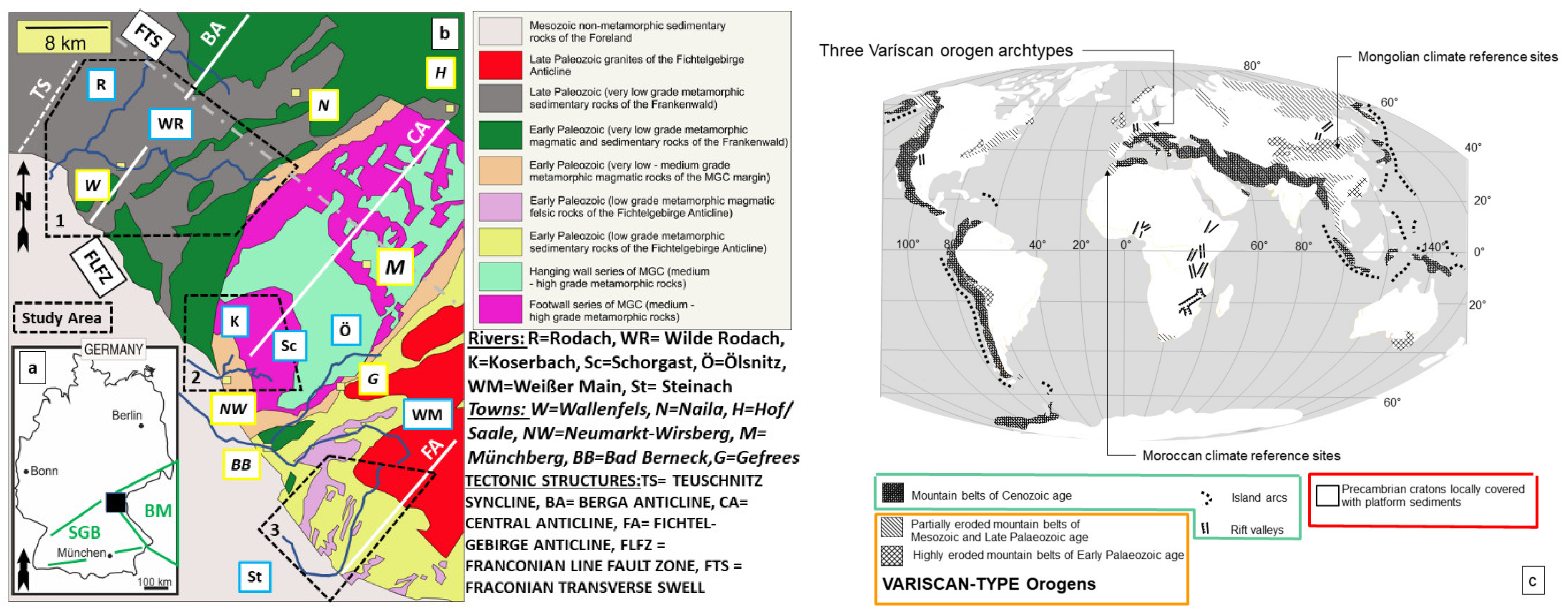
3. Geological and Geomorphological Setting
3.1. Geological Setting
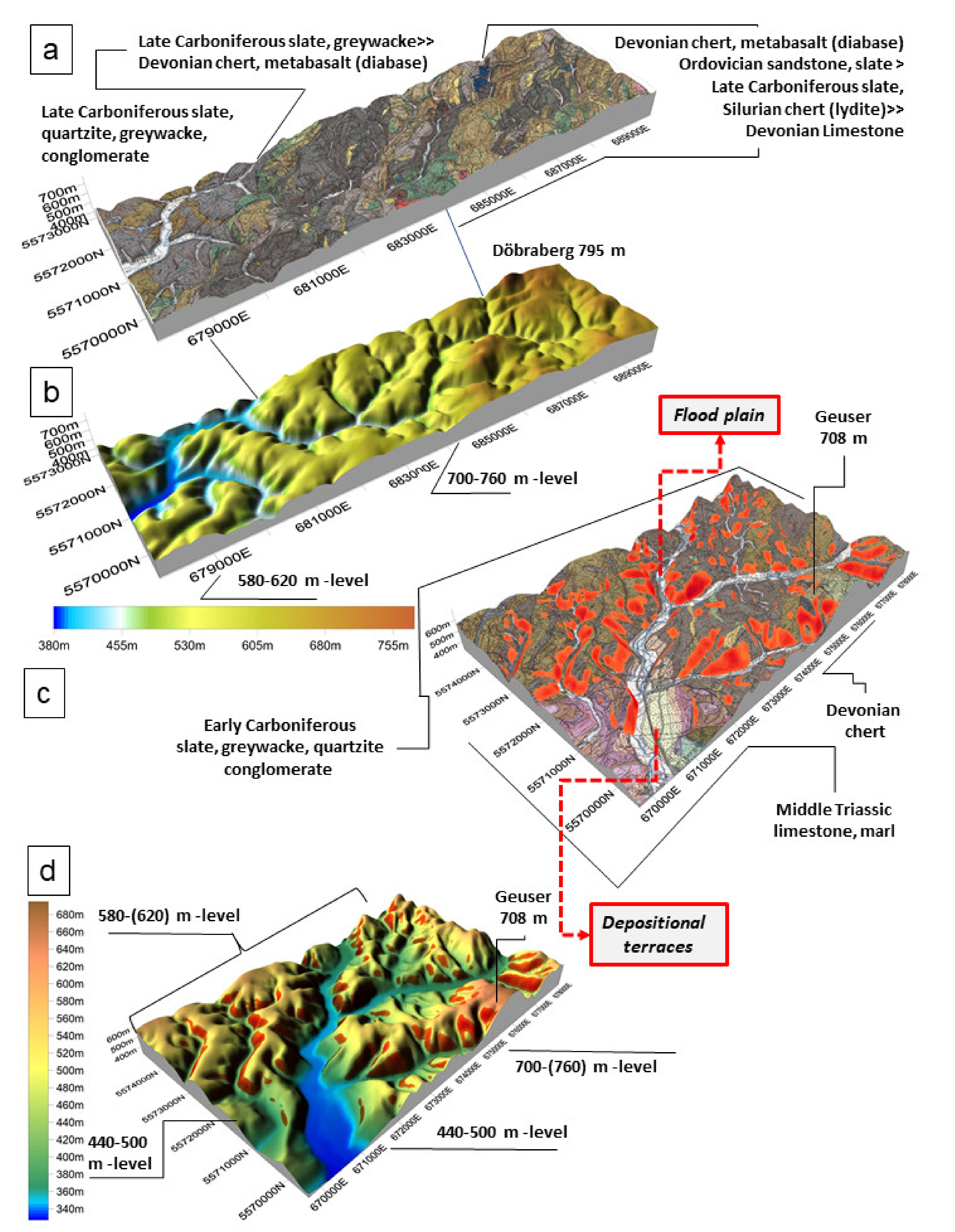
3.2. Geomorphological Setting
4. Results
4.1. Landforms—Identification, Mapping, and Interpretation
4.1.1. Definition and Classification of the Drainage Basin
4.1.2. Fluvial Processes and Their Landforms
4.1.3. Mass Wasting and Cryogenic Processes and Their Landforms
4.2. Hydrography of Drainage Systems vs. Compositional and Structural Variations of the Bedrock
4.2.1. Tectonics and Bedrock Lithology in the Study Areas
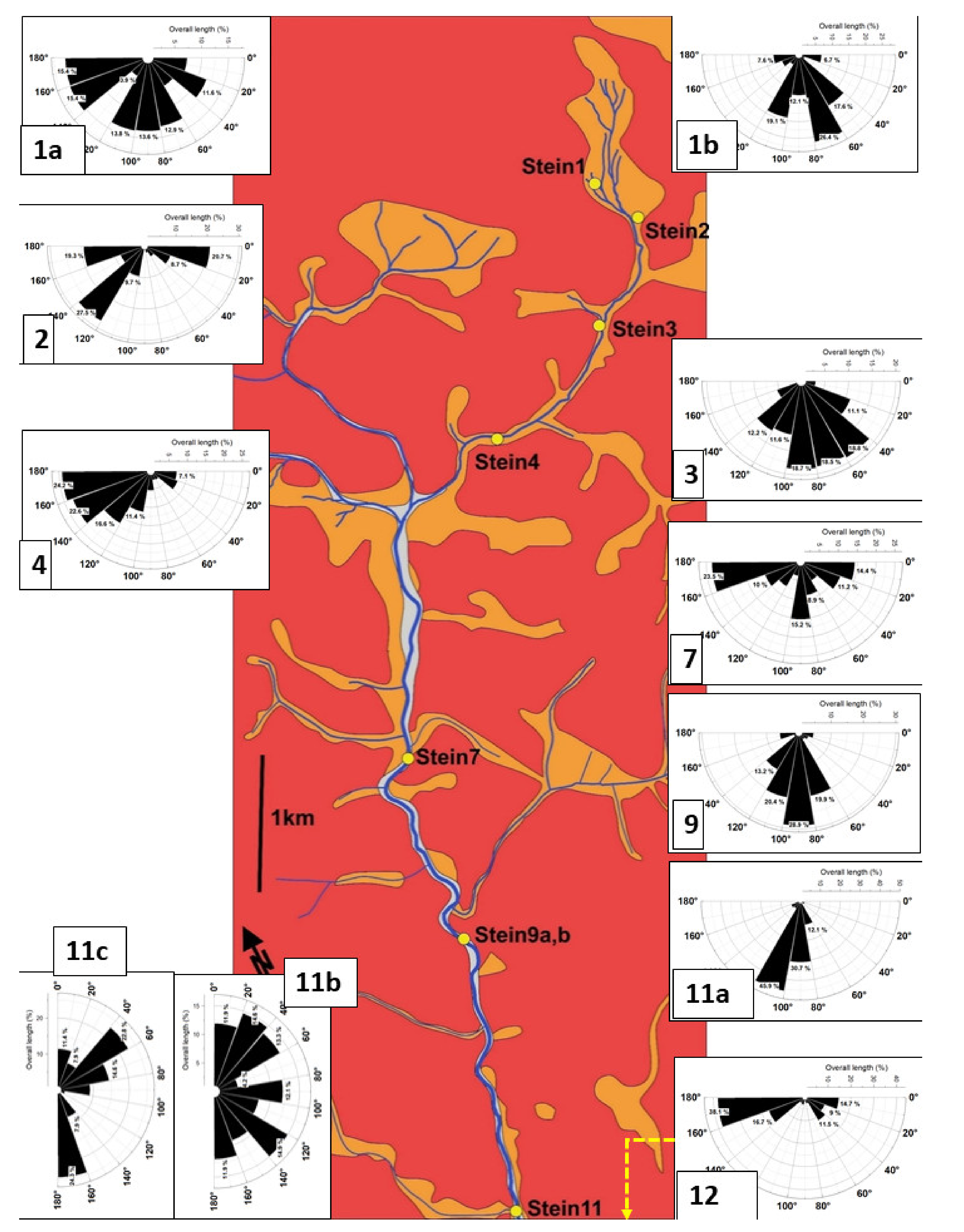
4.2.2. Channel Network and Structural Geology
4.2.3. Degree of Sinuosity and Drainage Classification
4.2.4. Channel Density and Channel Floodplain Ratio
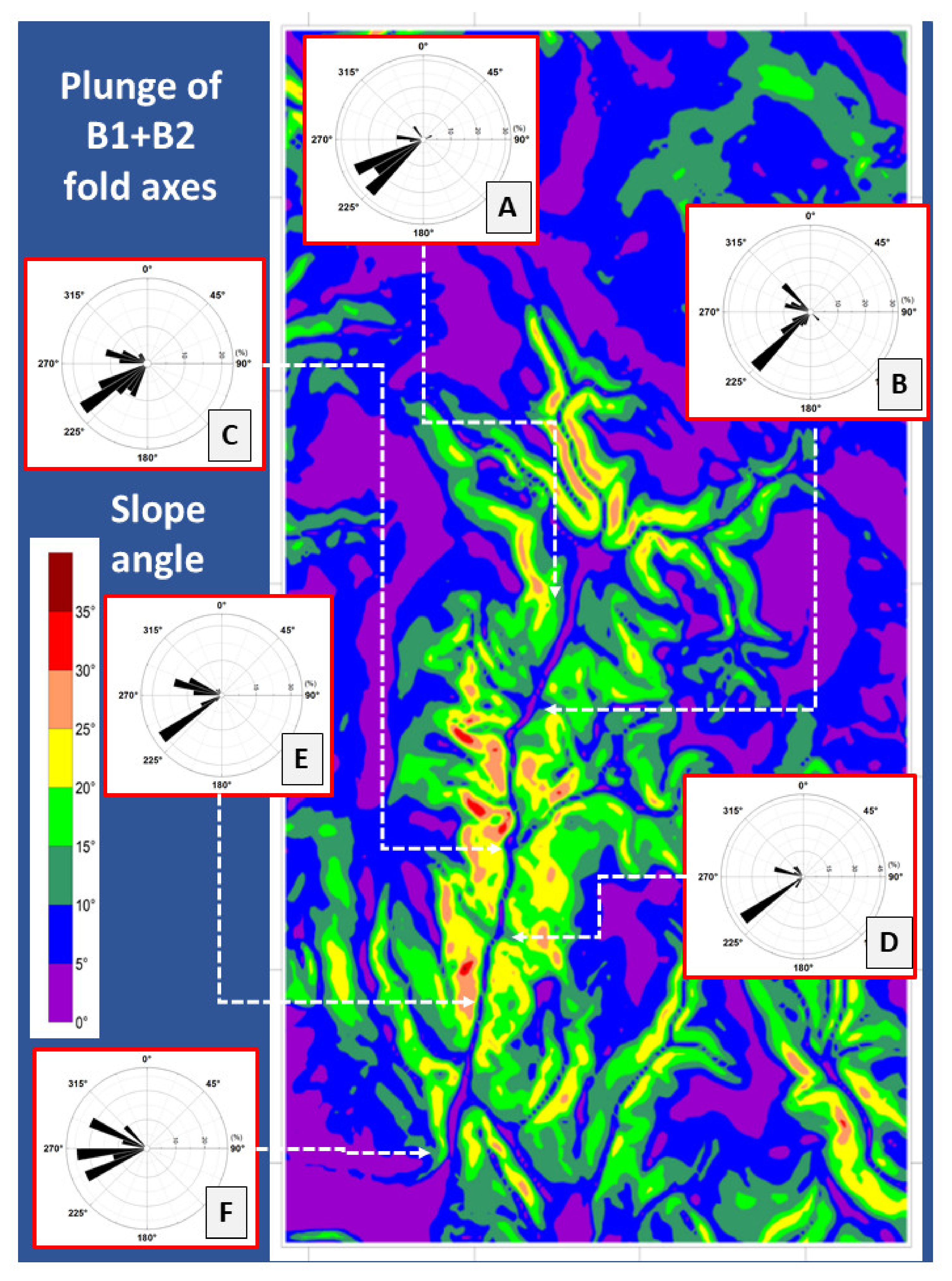
4.2.5. Slope Morphology vs. Bedrock-Lithology and Tectonic
4.3. Hydrodynamics and Grain Parameters (GMS Tool)
4.4. The Composition of Autochthonous and Allochthonous Mineralization of the SSS
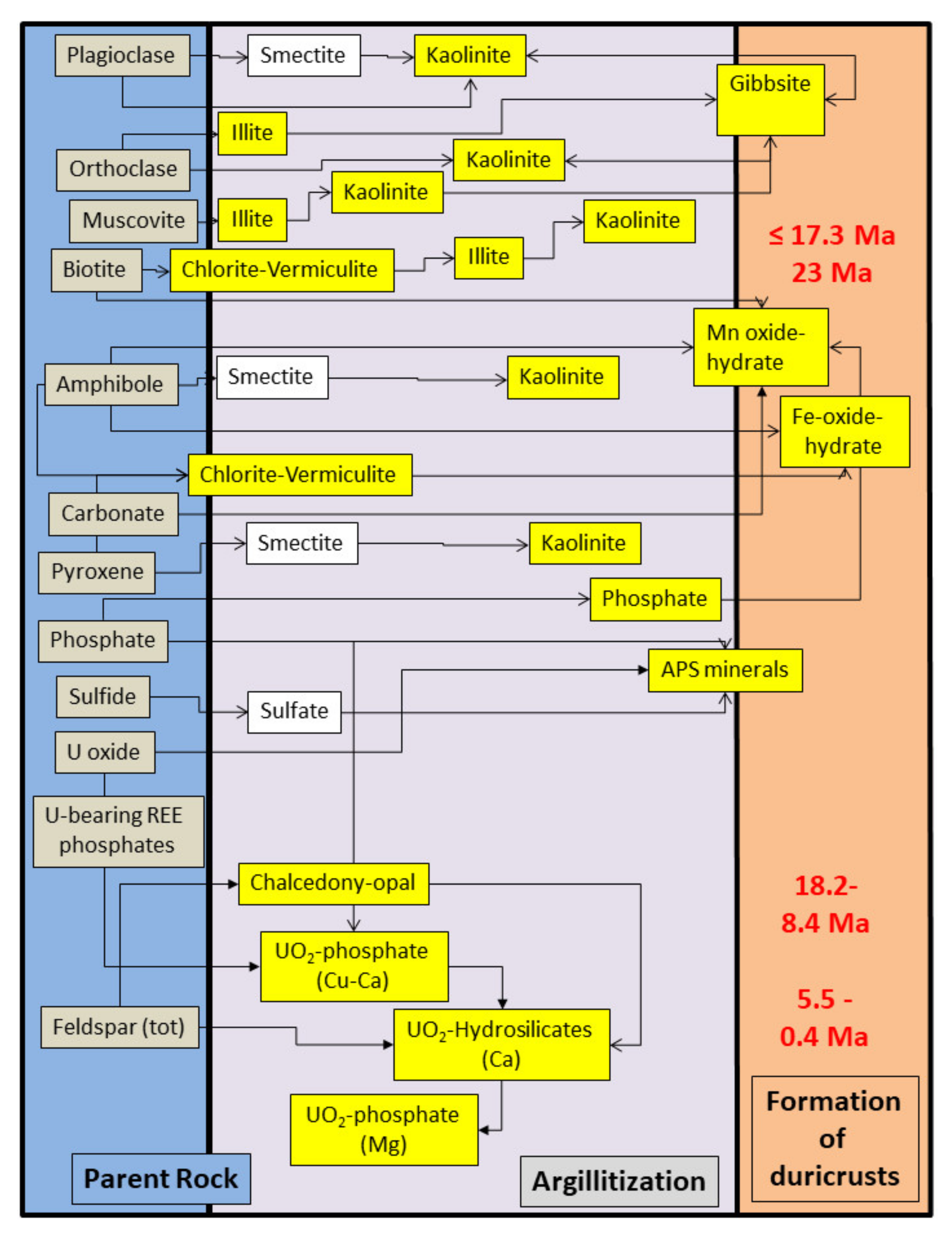
4.4.1. Composition and Age of Formation of the Mineral Association of the Supergene Alteration
4.4.2. Thickness and Variation of Autochthonous Mineralization
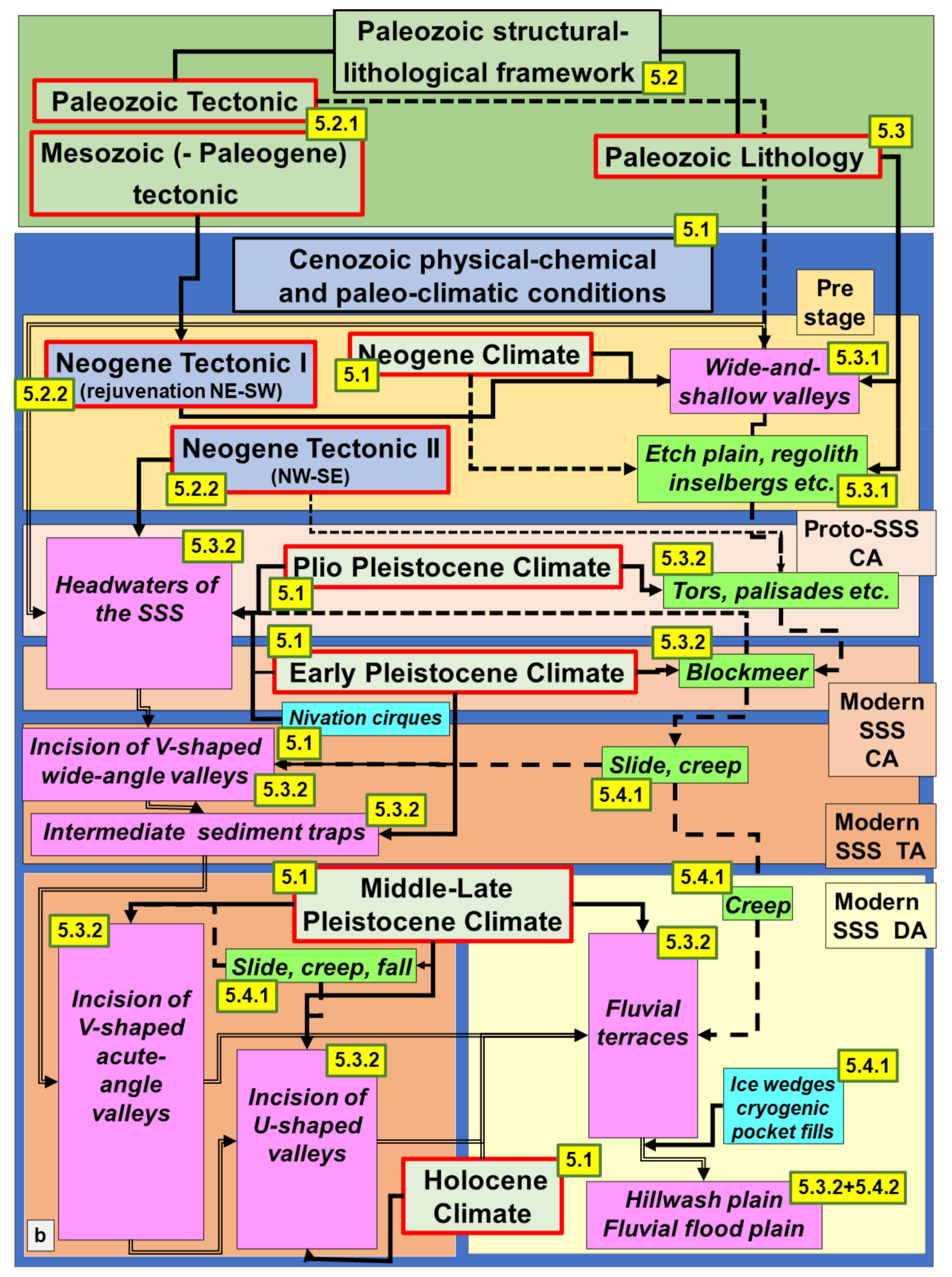
5. Discussion
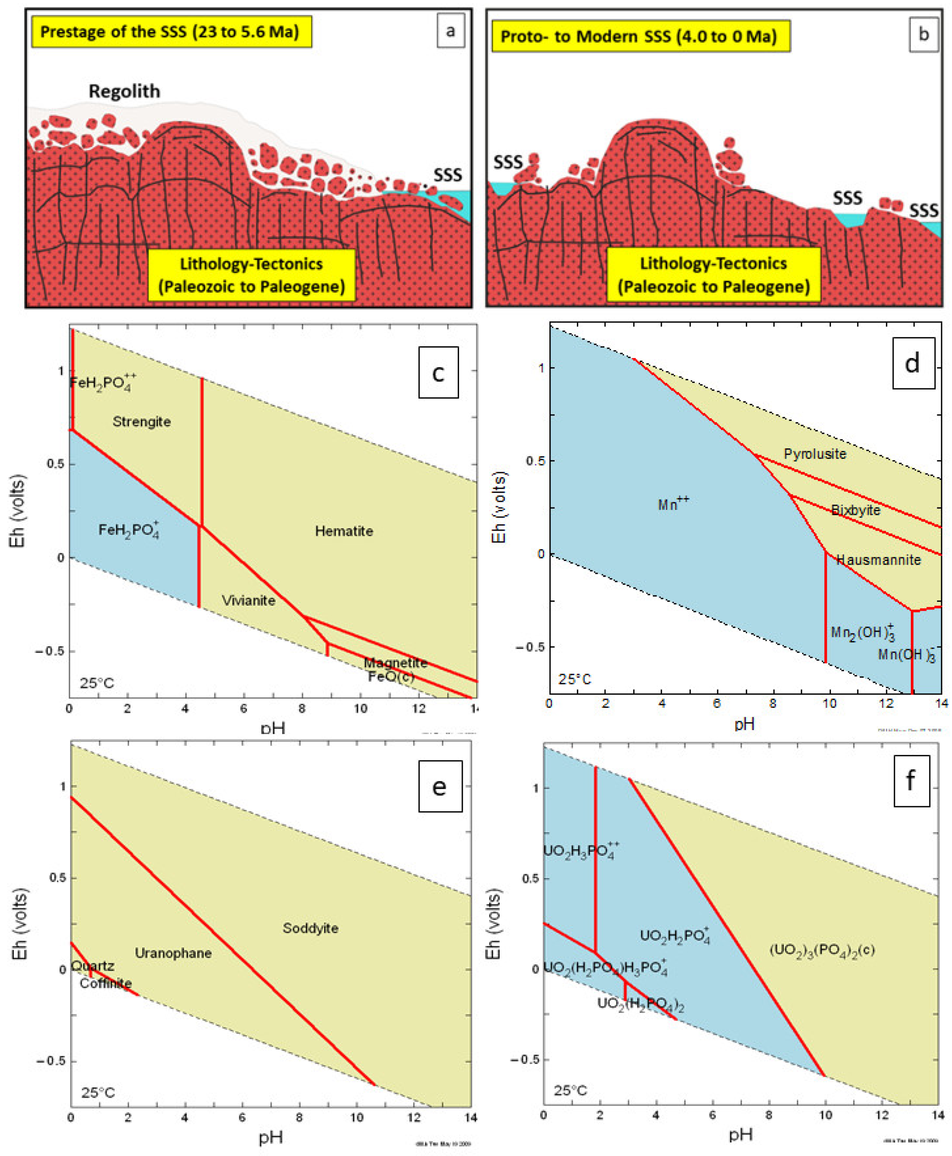
5.1. The Physical-Chemical Conditions and the Paleo-Climatic Regime
5.2. Maintenance of a Metastable Hydrodynamic State Needs the Constraints of a Structural-Lithological Framework and Effective Drivers
5.2.1. The Paleozoic Tectonic Framework
5.2.2. The Cenozoic Tectonic Driver
5.3. The Lithological Impact on the SSS
5.3.1. Bedrock Geology—Strongly Altered by the Climate
5.3.2. Bedrock Geology—Unaltered to Slightly Altered by the Climate
5.4. The Sediment Load and Its Implication on the Drainage System of the SSS
5.4.1. Hydrodynamic Regime and the GMS Tool
5.4.2. Lithology and Suspended Load
5.4.3. Lithology and Bedload
5.5. The SSS in View of Geodynamics and Crustal Maturity
5.6. The SSS in View of Higher and Lower Latitude Climate Zones
6. Conclusions
- The “key message” to the evolution of the SSS is as follows (Table 5, Figure 2b): The SSS analyzed in this study are metastable drainage systems which are maintained over a longer period of time (approx. 25 Ma) and distance from source to confluence (approx. 30 km) by a rigid framework provided by the tectonics and bedrock lithology. The SSS is kept operating by a climate change from humid tropical through periglacial into humid temperate. In terms of chronology, it is most suitably described by a four-stage succession.
- The geological framework of the SSS: Forming the lithological and structural features in the bedrock as a result of different temperature, pressure and dynamic metamorphic processes.
- Prestage of SSS: Forming the paleo-landscape with a stable fluvial regime as starting point for the SSS
- Proto-SSS: Transition into the metastable fluvial regime of the SSS
- Modern SSS: Operation of the metastable fluvial regime with the tendency to regain a stable hydrodynamic state in the adjacent foreland
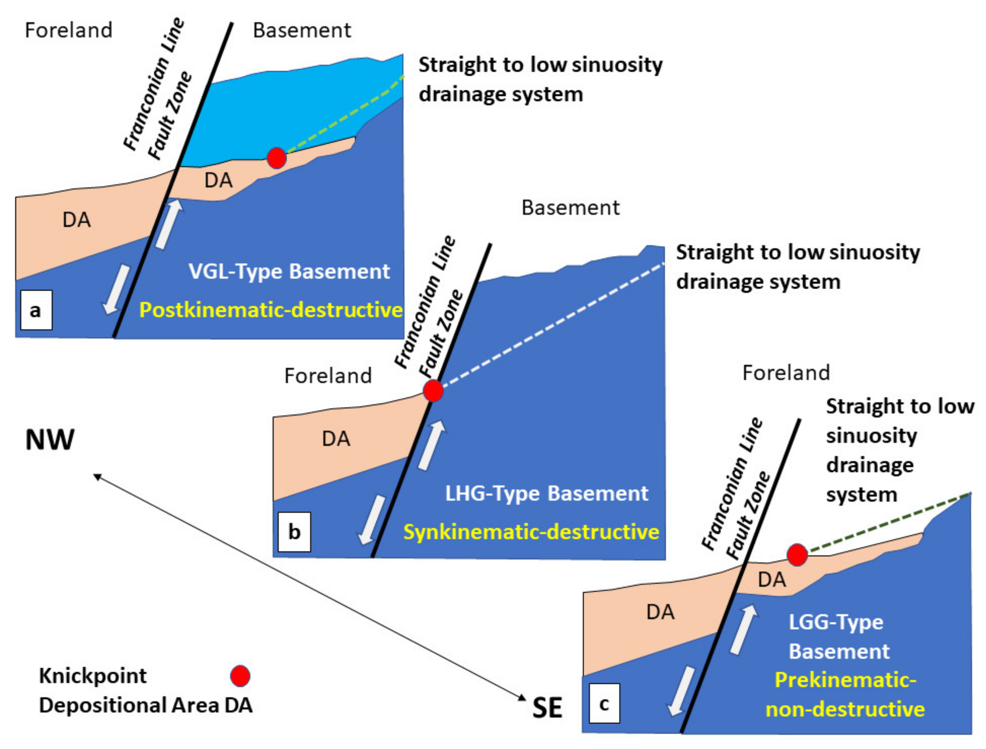
- Tectonics plays a dual role. Late Paleozoic fold tectonic affects the Paleozoic bedrock and creates the basis for the drainage pattern of these SSS. Its influence diminishes from the very-low-grade to the high-grade stage of metamorphism (VLG⇒LGG⇒LHG). So does its guiding effect on the emplacement of the drainage systems during the Neogene and Quaternary. Late Cenozoic fault tectonic triggered the onset of the SSS to incise into the basement. The impact of fault tectonic on the SSS depends on the vertical displacement that correlates with the fluvial gradient of the SSS, the development of knickpoints, the occurrence of intermediate sediment traps and the cross-sectional shape of valleys.
- The change in the bedrock lithology has an impact on the fluvial and colluvial sediments and their pertinent landforms. From slate to mica-gneiss (VLG⇒LGG⇒LHG) the vulnerability to chemical weathering increases and as a consequence of this a change among the process-related sediments takes place: gravel ⇒ clay + silt. The change of landforms follows suit: drainage system of straight ⇒ higher sinuosity and paired terraces ⇒ hillwash plains.
- The climate change has a mediating effect via the bedrock controlling the intensity of mechanical and chemical weathering. The first type of supergene alteration increases towards younger intervals, whereas the second one shows a decreasing trend. Together with the Cenozoic tectonic, climate governs the intensity of fluvial, colluvial and cryogenic land-forming processes.
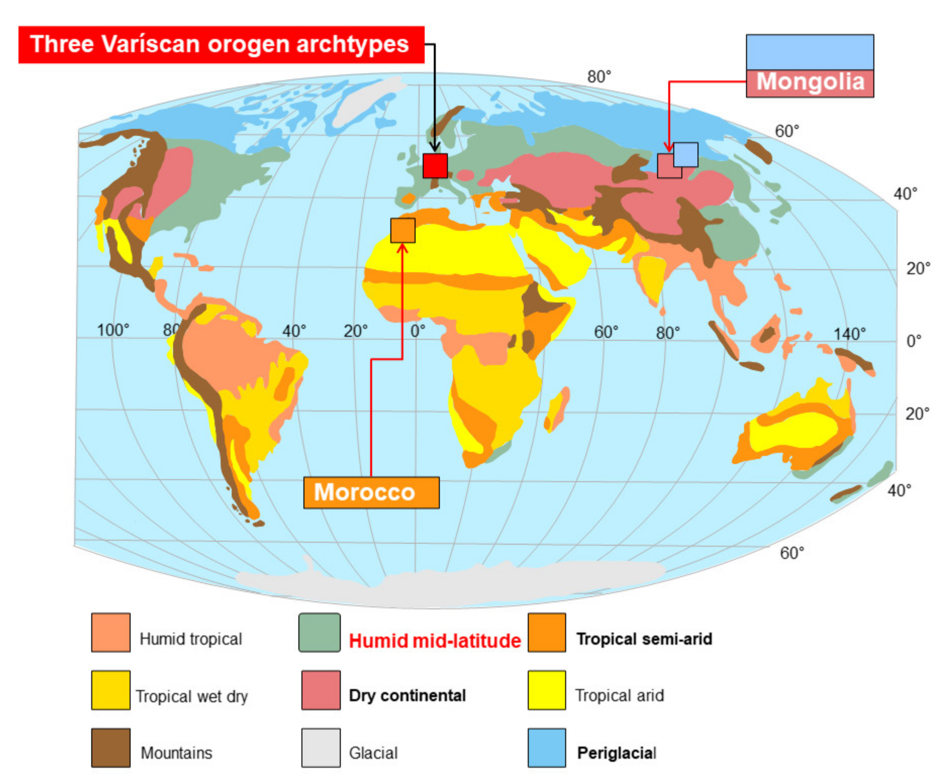
- The elaborated genetic model of the SSS is restricted to the basement of the Variscan -Type orogens which are representative of an intermediate maturity state between the pre-mature Cenozoic fold belts and the super-mature Precambrian cratons.
- Geomorphological-geological mapping of the fluvial, colluvial and cryogenic landform types is the descriptive part of the study while capturing numerical data relevant for the hydrographic studies of the SSS each reference area forms the geomorphometric one: (1) Quantification of fluvial and colluvial deposits along the drainage system, (2) slope angles, (3) degree of sinuosity as a function of river facies, (4) grain size distribution, (5) grain morphological categorization, (6) grain orientation (“situmetry”), (7) channel density, (8) channel/floodplain ratios.
- The compositional approach involves new mineralogical for the regolith which has been subdivided into a zone of argillitization and duricrusts. Their mineral assemblages are the basis for the thermodynamic computations (Eh, pH, concentration of solubles) to constrain the paleoclimatic regime during formation of the SSS.
- Comparing Variscan-type drainage systems from higher and lower-latitude climate zones relative to the archetypes reveals, the physical part (landform) of the SSS is controlled by tectonic and bedrock, whereas its chemical part (sediment composition) by the climate/weathering interacting with the country rocks.
Author Contributions
Funding
Data Availability Statement
Acknowledgments
Conflicts of Interest
References
- Williams, G.P. River meanders and channel size. J. Hydrol. 1986, 88, 147–164. [Google Scholar] [CrossRef]
- Miall, A.D. The Geology of Fluvial Deposits; Springer: New York, NY, USA, 1996; 582p. [Google Scholar]
- Knighton, D.A. Fluvial Forms and Processes: A New Perspective; Arnold: London, UK, 1998; 400p. [Google Scholar]
- Nanson, G.C.; Knighton, A.D. Anabranching rivers: Their cause, character and classification. Earth Surf. Process. Landf. 1996, 21, 217–239. [Google Scholar] [CrossRef]
- Selley, R.C. Applied Sedimentology, 2nd ed.; Academic Press: New York, NY, USA, 2000; 523p. [Google Scholar]
- Chin, A. The periodic nature of step-pool mountain streams. Am. J. Sci. 2002, 302, 144–167. [Google Scholar] [CrossRef]
- Moody, J.A.; Troutman, B.M. Characterization of the spatial variability of channel morphology. Earth Surf. Process. Landf. 2002, 27, 1251–1266. [Google Scholar] [CrossRef]
- Bridge, J.S. Rivers and Floodplains; Whiley-Blackwell: Oxford, UK, 2003; 504p. [Google Scholar]
- Robert, A. River Processes: An Introduction to Fluvial Dynamics; Routledge: Abingdon, UK, 2003; 238p. [Google Scholar]
- Charlton, R. Fundamentals of Fluvial Geomorphology; Routledge: Abingdon, UK, 2014; 214p. [Google Scholar]
- Wang, S.; Ni, J. Straight river: Its formation and speciality. J. Geogr. Sci. 2002, 12, 72–80. [Google Scholar]
- Audemard, F.A. Morpho-structural expression of active thrust fault systems in the humid tropical foothills of Colombia and Venezuela. Zeitschrift für Geomorphologie Supplementband 1999, 118, 227–244. [Google Scholar]
- Whipple, K. Bedrock rivers and the geomorphology of active orogens. Annu. Rev. Earth Planet. Sci. 2004, 32, 151–185. [Google Scholar] [CrossRef]
- Castillo, M.; Munoz-Salinas, E.; Ferrari, L. Response of a landscape to tectonics using channel steepness indices (ksn) and OSL: A case of study from the Jalisco Block, Western Mexico. Geomorphology 2014, 221, 204–214. [Google Scholar] [CrossRef]
- Gong, Z.; Li, S.; Li, B. The evolution of a terrace sequence along the Manas River in the northern foreland basin of Tian Shan, China, as inferred from optical dating. Geomorphology 2014, 213, 201–212. [Google Scholar] [CrossRef]
- Papanikolaou, I.D.; Van Balen, R.; Silva, P.G.; Reicherter, K. Geomorphology of active faulting and seismic hazard assessment: New tools and future challenges. Geomorphology 2015, 237, 1–13. [Google Scholar] [CrossRef]
- Zondervan, J.R.; Stokes, M.; Boulton, S.J.; Telfer, M.W.; Mather, A.E. Rock strength and structural controls on fluvial erodibility: Implications for drainage divide mobility in a collisional mountain belt. Earth Planet. Sci. Lett. 2020, 538, 116221. [Google Scholar] [CrossRef]
- Sancho, C.; Pena, J.L.; Rivelli, F.; Rhodes, E.; Munoz, A. Geomorphological evolution of the Tilcara alluvial fan (Jujuy Province, NW Argentina): Tectonic implications and palaeoenvironmental considerations. J. S. Am. Earth Sci. 2008, 26, 68–77. [Google Scholar] [CrossRef]
- Stokes, M.; Mather, A.E.; Belfoul, A.; Farik, F. Active and passive tectonic controls for transverse drainage and river gorge development in a collisional mountain belt (Dades Gorges, High Atlas Mountains, Morocco). Geomorphology 2008, 102, 2–20. [Google Scholar] [CrossRef]
- Perez-Pena, J.V.; Azor, A.; Azanon, J.M.; Keller, E.A. Active tectonics in the Sierra Nevada (Betic Cordillera, SE Spain): Insights from geomorphic indexes and drainage pattern analysis. Geomorphology 2010, 119, 74–87. [Google Scholar] [CrossRef]
- Burbank, D.; Anderson, R. Tectonic Geomorphology; John Wiley & Sons: New York, NY, USA, 2011; 274p. [Google Scholar]
- Molin, P.; Fubelli, G.; Nocentini, M.; Sperini, S.; Ignat, P.; Grecu, F.; Dramis, F. Interaction of mantle dynamics, crustal tectonics and surface processes in the topography of the Romanian Carpathians: A geomorphological approach. Glob. Planet. Chang. 2012, 90, 58–72. [Google Scholar] [CrossRef]
- García, V.; Hongn, F.; Cristallini, E. Late Miocene to recent morphotectonic evolution and potential seismic hazard of the northern Lerma valley: Clues from Lomas de Medeiros, Cordillera Oriental, NW Argentina. Tectonophysics 2013, 608, 1238–1253. [Google Scholar] [CrossRef]
- Jelínek, J.; Staněk, F.; Thomas, J.; Daněk, T.; Mališ, J. The application of morphostructural analysis and its validation by comparison with documented faults within the Zlaté Hory ore district (the Northeastern part of the Bohemian Massif). Acta Geodyn. Geomater. 2013, 10, 5–17. [Google Scholar] [CrossRef]
- Melosh, B.L.; Keller, E.A. Effects of active folding and reverse faulting on stream channel evolution, Santa Barbara Fold Belt, California. Geomorphology 2013, 186, 119–135. [Google Scholar] [CrossRef]
- Milliman, J.D.; Syvitski, J.P.M. Geomorphic/tectonic control of sediment discharge to the ocean: The importance of small mountainous rivers. J. Geol. 1992, 100, 525–544. [Google Scholar] [CrossRef]
- Harbor, D.J.; Schumm, S.A.; Harvey, M.D. Tectonic control of the Indus River in Sindh, Pakistan. In The Variability of Large Alluvial Rivers; Schumm, S.S., Winkley, B.R., Eds.; American Association of Civil Engineers Press: New York, NY, USA, 1994; pp. 161–176. [Google Scholar]
- Ruddiman, W.F. Tectonic Uplift and Climate Change; Springer: New York, NY, USA, 1997; 556p. [Google Scholar]
- Tinkler, K.J.; Wohl, E.E. Rivers over Rock: Fluvial Processes in Bedrock Channels; Geophysical Monograph; John Wiley & Sons: New York, NY, USA, 1998; Volume 107, 323p. [Google Scholar]
- Wohl, E.E. Bedrock channel morphology in relation to erosional processes. In Rivers Over Rock: Fluvial Processes in Bedrock Channels; Geophysical Monograph Series; Tinkler, K.J., Wohl, E.E., Eds.; American Geophysical Union: Washington, DC, USA, 1998; pp. 133–151. [Google Scholar]
- Schumm, S.A. Active Tectonics and Alluvial Rivers; Cambridge University Press: Cambridge, UK, 2000; 290p. [Google Scholar]
- Leeder, M. Sedimentology and Sedimentary Basins: From Turbulence to Tectonics; John Wiley & Sons: New York, NY, USA, 2011; 794p. [Google Scholar]
- Gutiérrez, F.; Gutiérrez, M. Landforms of the Earth; Springer: New York, NY, USA, 2016; 284p. [Google Scholar]
- Kasanin-Grubin, M.; Yair, A.; Romero, E.N.; Vergari, F.; Troiani, F.; Desloges, J.; Yan, L.; Moreno de las Heras, M.; Della Seta, M.; Hardenbicker, U.M.; et al. 2018 The role of lithological properties on badland development. In Geophysical Research Abstracts 21; EGU 2019-1021; EGU General Assembly: Vienna, Austria, 2019; Volume 21, p. 1. [Google Scholar]
- Emmert, U.; Horstig, G.V.; Stettner, G. Geologische Übersichtkarte 1:200000 CC 6334 Bayreuth; BGR: Hannover, Germany, 1981. [Google Scholar]
- Summerfield, M.A. Global Geomorphology; John Wiley and Sons Inc.: New York, NY, USA, 1991; 537p. [Google Scholar]
- Easterbrook, D.J. Surface Processes and Landforms, 2nd ed.; Prentice Hall: New York, NY, USA, 1999; 546p. [Google Scholar]
- McCann, T. The Geology of Central Europe: Precambrian and Paleozoic: 1; Special Volume; The Geological Society of London: London, UK, 2008; 748p. [Google Scholar]
- McCann, T. The Geology of Central Europe: Mesozoic and Cenozoic: 2; Special Volume; The Geological Society of London: London, UK, 2008; 700p. [Google Scholar]
- Bates, R.L.; Jackson, J.A. Glossary of Geology; American Geological Institute: Alexandria, VA, USA, 2005; 779p. [Google Scholar]
- Evans, I.S.; Minár, J. A classification of geometric variables. Geomorphometry 2011, 2011, 105–107. [Google Scholar]
- Dill, H.G.; Ludwig, R.-R.; Kathewera, A.; Mwenelupembe, J. A lithofacies terrain model for the Blantyre Region: Implications for the interpretation of palaeo savanna depositional systems and for environmental geology and economic geology in southern Malawi. J. Afr. Earth Sci. 2005, 41, 341–393. [Google Scholar] [CrossRef]
- Callahan, J. A nontoxic heavy liquid and inexpensive filters for separation of minerals grains. J. Sediment. Petrol. 1987, 57, 765–766. [Google Scholar] [CrossRef]
- Brookins, D.G. Eh-pH Diagrams for Geochemistry; Springer: Heidelberg, Germany, 1987; 176p. [Google Scholar]
- Geyh, M.A.; Schleicher, H. Absolute Age Dating Determination Physical and Chemical Dating Methods and Their Application; Springer: Berlin, Germany, 1990; 63p. [Google Scholar]
- Wallinga, J. Optically luminescence dating of fluvial deposits: A review. Boreas 2002, 31, 303–322. [Google Scholar] [CrossRef]
- Onac, B.P. Mineralogical studies and Uranium-series dating of speleothems from Scåricoara Glacier Cave (Bihor Mountains, Romania). Theor. Appl. Karstology 2001, 13, 33–38. [Google Scholar]
- Dill, H.G.; Hansen, B.; Keck, E.; Weber, B. Cryptomelane a tool to determine the age and the physical-chemical regime of a Plio-Pleistocene weathering zone in a granitic terrain (Hagendorf, SE Germany). Geomorphology 2010, 121, 370–377. [Google Scholar] [CrossRef]
- Dill, H.G.; Gerdes, A.; Weber, B. Age and mineralogy of supergene uranium minerals—Tools to unravel geomorphological and palaeohydrological processes in granitic terrains (Bohemian Massif, SE Germany). Geomorphology 2010, 117, 44–65. [Google Scholar] [CrossRef]
- Dill, H.G.; Wemmer, K. Origin and K/Ar age of cryptomelane-bearing Sn placers on silcretes, SE Germany. Sediment. Geol. 2012, 275, 70–78. [Google Scholar] [CrossRef]
- Dill, H.G.; Wehner, H. The depositional environment and mineralogical and chemical compositions of high ash brown coal resting on early Tertiary saprock (Schirnding Coal Basin, SE Germany). Int. J. Coal Geol. 1999, 39, 301–328. [Google Scholar] [CrossRef]
- Horacio, J. River sinuosity index: Geomorphological characterization. In Technical Note 2 CIREF and Wetlands International; Physical Geography, Santiago de Compostela University: Santiago de Compostela, Spain, 2014; 6p. [Google Scholar]
- Turowski, J.M. Alluvial cover controlling the width, slope and sinuosity of bedrock channels. Earth Surf. Dyn. 2018, 6, 29–48. [Google Scholar] [CrossRef]
- Ahnert, F.O. Einführung in Die Geomorphologie; UTB GmbH: Stuttgart, Germany, 2015; 458p. [Google Scholar]
- Nelson, F.E. A preliminary investigation of solifluction macrofabrics. Catena 1985, 12, 23–33. [Google Scholar] [CrossRef]
- Nieuwenhuijzen, M.E.; Van Steijn, H. Alpine debris flows and their sedimentary properties. A case study from the French Alps. Permafr. Periglac. Process. 1990, 1, 111–128. [Google Scholar] [CrossRef]
- Millar, S.W.; Nelson, F.E. Sampling-surface orientation and clast macrofabric in periglacial colluviums. Earth surface pro-cesses and landforms. Earth Surf. Process. Landf. 2001, 26, 523–529. [Google Scholar] [CrossRef]
- Lindsey, D.A.; Langer, W.H.; Van Gosen, B.S. Using pebble lithology and roundness to interpret gravel provenance in pied-mont fluvial systems of the Rocky Mountains, USA. Sediment. Geol. 2007, 199, 223–232. [Google Scholar] [CrossRef]
- Dill, H.G. Geology and chemistry of Variscan-type pegmatite systems (SE Germany)—With special reference to structural and chemical pattern recognition of felsic mobile components in the crust. Ore Geol. Rev. 2018, 92, 205–239. [Google Scholar] [CrossRef]
- Illenberger, W.K. Pebble shape (and size?). J. Sediment. Res. 1991, 61, 756–767. [Google Scholar]
- Dill, H.G.; Ulrich, H.-J. Geoelectric deep sounding—A contribution to constrain the genesis of siliceous ferromanganese duri-crusts on deeply weathered Palaeozoic basement rocks (N. Bavaria, F.R. Germany). Z. Geomorphol. 1987, 31, 361–370. [Google Scholar] [CrossRef]
- Dill, H.G.; Buzatu, A.; Balaban, S.-I.; Ufer, K.; Techmer, A.; Schedlinsky, W.; Füssl, M. The transition of very coarse-grained meandering to straight fluvial drainage systems in a tectonized foreland-basement landscape during the Holocene (SE Germany)—A joint geomorphological-geological study. Geomorphology 2020, 370, 107364. [Google Scholar] [CrossRef]
- Zöller, L.; Beierkuhnlein, C.; Samimi, C.; Faust, D. Die Physische Geographie Deutschlands; WBG—Wissenschaftliche Buchgesellschaft: Darmstadt, Germany, 2017; 208p. [Google Scholar]
- Thauer, W. Morphologische Studien im Frankenwald und im Frankenwaldvorland. Mitt. Fränkischen Geogr. Ges. 1954, 1, 168–169. [Google Scholar]
- Strebel, O. Tertiäre Reliktböden, Tertiäre Verwitterungsreste und Eiszeitliche Bodenumlagerungen im Frankenwald. Ph.D. Thesis, Universität Würzburg, Würzburg, Germany, 1955; 53p. [Google Scholar]
- Drexler, O. Das Espich-Sediment bei Kulmbach. Bayreuther Geowiss. Arb. 1980, 1, 9–38. [Google Scholar]
- Kleber, A.; Stingl, H. Zur Flußgeschichte des Trebgasttals nördlich von Bayreuth. Eine zweiphasige Talverlegung im Rotmainsystem. In Beiträge zur Landeskunde Oberfrankens. Festschrift zum 65. Geburtstag von Bezirkstagspräsidenten Edgar Sitzmann; Becker, H., Ed.; University Bamberg: Bamberg, Germany, 2000; pp. 191–208. [Google Scholar]
- Zöller, L.; Stingl, H.; Kleber, A. Das Trebgasttal—Tal- und Landschaftsentwicklung nahe der Europäischen Hauptwasserscheide im Raum Bayreuth. Bayreuther Geogr. Arb. 2007, 28, 70–101. [Google Scholar]
- Schirmer, W. Die Geschichte von Moenodanuvius und Main in Oberfranken. In Streifzüge Durch Franken Band; Dippold, G., Ed.; Lichtenfels: Lichtenfels, Germany, 2010; Volume 1, pp. 9–24. [Google Scholar]
- Bucher, K.; Grapes, R. Petrogenesis of Metamorphic Rocks; Springer Science & Business Media: New York, NY, USA, 2011; 428p. [Google Scholar]
- Stettner, G. Geologische Karte von Bayern 1:25,000 Erläuterung Blatt 5936 Bad Berneck München; Geologisches Landesamt: München, Germany, 1977; 225p. [Google Scholar]
- Kennan, L.; Lamb, S.H.; Hoke, L. High-altitude palaeosurfaces in the Bolivian Andes: Evidence for late Cenozoic surface uplift. Spec. Publ. Geol. Soc. Lond. 1997, 120, 307–323. [Google Scholar] [CrossRef]
- Babault, J.; Bonnet, S.; Driessche, J.V.D.; Crave, A. High elevation of low-relief surfaces in mountain belts: Does it equate to post-orogenic surface uplift? Terra Nova 2007, 19, 272–277. [Google Scholar] [CrossRef]
- Landis, C.A.; Campbell, H.J.; Begg, J.G.; Mildenhall, D.C.; Paterson, A.M.; Trewick, S.A. The Waipounamu erosion surface: Questioning the antiquity of the New Zealand land surface and terrestrial fauna and flora. Geol. Mag. 2008, 145, 173–197. [Google Scholar] [CrossRef]
- Hall, A.M.; Ebert, K.; Kleman, J.; Nesje, A.; Ottesen, D. Selective glacial erosion on the Norwegian passive margin. Geology 2013, 41, 1203–1206. [Google Scholar] [CrossRef]
- Migoń, P. Tertiary etch surfaces in the Sudetes Mountains, SW Poland: A contribution to the preQuaternary morphology of Central Europe”. In Palaeosurfaces: Recognition, Reconstruction and Palaeoenvironmental Interpretation; Special Publications; Widdowson, M., Ed.; Geological Society: London, UK, 1997; Volume 120, pp. 187–202. [Google Scholar]
- Büdel, J. Die “Doppelten Einebnungsflächen” in den feuchten Tropen. Z. Geomorphol. NF 1957, 1, 201–228. [Google Scholar]
- Jacobson, R.B.; Blevins, B.W.; Bitner, C.J. Sediment regime constraints on river restoration—An example from the Lower Missouri River. In Management and Restoration of Fluvial Systems with Broad Historical Changes and Human Impacts; James, L.A., Rathburn, S.L., Whittecar, G.R., Eds.; Geological Society of America Special Paper: Boulder, CO, USA, 2009; Volume 451, pp. 1–22. [Google Scholar]
- Emmert, U. Ein Beitrag zur Flußgeschichte des Frankenwaldes und seines Vorlandes im Bereich des Kartenblattes Stadtsteinach (1:25,000). Geol. Bl. NO-Bayern 1953, 3, 36–42. [Google Scholar]
- Emmert, U.; von Horstig, G. Geologische Karte von Bayern 1:25,000 Erläuterung Blatt 5734 Wallenfels München; Geologisches Landesamt: München, Germany, 1972; 240p. [Google Scholar]
- Emmert, U.; Stettner, G. Geologische Karte von Bayern 1:25,000 Erläuterung Blatt 6036 Weidenberg München; Geologisches Landesamt: München, Germany, 1995; 239p. [Google Scholar]
- Emmert, U.; Weinelt, W. Geologische Karte von Bayern 1:25,000 Erläuterung Blatt 5935 Marktschorgast München; Geologisches Landesamt: München, Germany, 1962; 286p. [Google Scholar]
- Bryan, R.; Yair, A. Perspectives on studies of badland geomorphology. In Badland Geomorphology and Piping; Bryan, R., Yair, A., Eds.; Geobooks: Norwick, UK, 1982; pp. 1–12. [Google Scholar]
- Dill, H.G.; Buzatu, A.; Goldmann, S.; Kaufhold, S.; Bîrgăoanu, D. Coastal landforms of “Meso-Afro-American” and “Neo-American” landscapes in the periglacial South Atlantic Ocean: With special reference to the clast orientation, morphology, and granulometry of continental and marine sediments. J. S. Am. Earth Sci. 2020, 98, 102385. [Google Scholar] [CrossRef]
- Rea, B.R.; Whalley, W.B.; Rainey, M.M.; Gordon, J.E. Blockfields, old or new? Evidence and implications from some plateaus in northern Norway. Geomorphology 1996, 15, 109–121. [Google Scholar] [CrossRef]
- Fjellanger, J.; Sørbel, L.; Linge, H.; Brook, E.J.; Raisbeck, G.M.; Yiou, F. Glacial survival of blockfields on the Varanger Peninsula, northern Norway. Geomorphology 2006, 82, 255–272. [Google Scholar] [CrossRef]
- Twidale, C.R.; Vidal Romani, J.R. Landforms and Geology of Granite Terrains; Taylor & Francis Ltd.: London, UK, 2005; 354p. [Google Scholar]
- Migoń, P. Granite Landscapes of the World. In Geomorphological Landscapes of the World 22; Oxford University Press: Oxford, UK, 2006; 416p. [Google Scholar]
- Migoń, P.; Thomas, M.F. Grus weathering mantles—Problems of interpretation. Catena 2002, 49, 5–24. [Google Scholar] [CrossRef]
- Shakesby, R.A. Pronival (protalus) ramparts: A review of forms, processes, diagnostic criteria and palaeoenvironmental implications. Prog. Phys. Geogr. 1997, 21, 394–418. [Google Scholar] [CrossRef]
- Matthews, J.A.; Wilson, P.; Mourne, R.W. Landform transitions from pronival ramparts to moraines and rock glaciers: A case study from the Smørbotn cirque, Romsdalsalpane, southern Norway. Geogr. Ann. Ser. A Phys. Geogr. 2017, 99, 15–37. [Google Scholar] [CrossRef]
- Watson, E. Two nivation cirques near Aberystwyth, Wales. Biul. Peryglac. 1966, 15, 79–101. [Google Scholar]
- Christiansen, H.H. Nivation forms and processes in unconsolidated sediments, NE Greenland. Earth Surf. Process Landforms 1998, 23, 751–760. [Google Scholar] [CrossRef]
- Raab, T.; Völkel, J. Late Pleistocene glaciation of the Kleiner Arbersee area in the Bavarian Forest, South Germany. Quat. Sci. Rev. 2003, 22, 581–593. [Google Scholar] [CrossRef]
- Ehlers, J.; Eissmann, L.; Lippstreu, L.; Stephan, H.-J.; Wansa, S. Pleistocene Glaciations of North Germany. Dev. Quat. Sci. 2 2004, 2, 135–145. [Google Scholar]
- Rinterknecht, V.; Matoshko, A.; Gorokhovich, Y.; Fabel, D.; Xu, S. Expression of the Younger Dryas cold event in the Carpa-thian Mountains, Ukraine. Quat. Sci. Rev. 2012, 39, 106–114. [Google Scholar] [CrossRef]
- Fiebig, M.; Buiter, S.J.H.; Ellwanger, D. Pleistocene glaciations of South Germany. Dev. Quat. Sci. 2 2004, 147–154. [Google Scholar]
- Fossen, H. Structural Geology; Cambridge University Press: Cambridge, UK, 2010; p. 480. [Google Scholar]
- Lisle, R.J.; Brabham, P.; Barnes, J.W. Basic Geological Mapping (Geological Field Guide), 5th ed.; John Wiley & Sons: New York, NY, USA, 2011; 230p. [Google Scholar]
- Seidel, G. Geologie von Thüringen; Schweitzerbartsche Verlagsbuchhandlung: Stuttgart, Germany, 1995; 556p. [Google Scholar]
- Kley, J. “Saxonian tectonics” in the 21st century. Z. Dtsch. Ges. Geowiss. 2013, 164, 295–311. [Google Scholar] [CrossRef]
- Ring, U.; Bolhar, R. Tilting, uplift, volcanism, and disintegration of the South German Block. Tectonophysics 2020, 795, 228611. [Google Scholar] [CrossRef]
- Emmert, U.; von Horstig, G.; Weinelt, W.i. Geologische Karte von Bayern 1:25,000 Erläuterung Blatt 5835 Stadtsteinach; München, Geologisches Landesamt: München, Germany, 1960; 279p. [Google Scholar]
- Von Horstig, G. Geologische Karte von Bayern 1:25,000 Erläuterung Blatt 5635 Nordhalben München; Geologisches Landesamt: München, Germany, 1966; 167p. [Google Scholar]
- Von Horstig, G.; Stettner, G. Geologische Karte von Bayern 1:25,000 Erläuterung Blatt 5636 Naila München; Geologisches Landesamt: München, Germany, 1962; 192p. [Google Scholar]
- Von Horstig, G.; Stettner, G. Geologische Karte von Bayern 1:25,000 Erläuterung Blatt 5736 Helmbrechts München; Geologisches Landesamt: München, Germany, 1970; 176p. [Google Scholar]
- Von Horstig, G.; Stettner, G. Geologische Karte von Bayern 1:25,000 Erläuterung Blatt 5735 Schwarzenbach a. Wald. München; Geologisches Landesamt: München, Germany, 1976; 178p. [Google Scholar]
- Štěpančíková, P.; Stemberk, J.; Vilímek, V.; Košťák, B. Neotectonic development of drainage networks in the East Sudeten Mountains and monitoring of recent fault displacements (Czech Republic). Geomorphology 2008, 102, 68–80. [Google Scholar] [CrossRef]
- Vita-Finzi, C. Recent Earth Movements: An Introduction to Neotectonics; Academic Press: Cambridge, UK, 1986; 226p. [Google Scholar]
- Schumm, S.A. Sinuosity of alluvial channels on the Great Plains. Geol. Soc. Am. Bull. 1963, 74, 1089–1100. [Google Scholar] [CrossRef]
- Church, M. Geomorphic thresholds in riverine landscapes. Freshw. Biol. 2002, 47, 541–557. [Google Scholar] [CrossRef]
- Beechie, T.J.; Liermann, M.; Pollock, M.M.; Baker, S.; Davies, J. Channel pattern and river-floodplain dynamics in forested mountain river systems. Geomorphology 2006, 78, 124–141. [Google Scholar] [CrossRef]
- Hack, J.T. Stream-Profile Analysis and Stream-Gradient Index. J. Res. U. S. Geol. Surv. 1973, 1, 421–429. [Google Scholar]
- Gomez, F.; Barazangi, M.; Bensaid, M. Active tectonism in the intracontinental Middle Atlas Mountains of Morocco: Syn-chronous crustal shortening and extension. J. Geol. Soc. Lond. 1996, 153, 389–402. [Google Scholar] [CrossRef]
- Zuchiewicz, W. Time-series analysis of river bed gradients in the Polish Carpathians: A statistical approach to the studies on young tectonic activity. Z. Geomorphol. 1995, 39, 461–477. [Google Scholar] [CrossRef]
- Demoulin, A. Testing the tectonic significance of some parameters of longitudinal river profiles: The case of the Ardenne (Bel-gium, NW Europe). Geomorphology 1998, 24, 189–208. [Google Scholar] [CrossRef]
- Dill, H.G.; Buzatu, A.; Balaban, S.-I.; Ufer, K.; Gómez Tapias, J.; Bîrgăoanu, D.; Cramer, T. The “badland trilogy” of the Desierto de la Tatacoa, Upper Magdalena Valley, Colombia, a result of geodynamics and climate: With a review of badland landscapes. Catena 2020, 194, 104696. [Google Scholar] [CrossRef]
- Pettijohn, F.J.; Potter, P.E.; Siever, R. Sand and Sandstone; Springer: Berlin, Germany, 1987; 553p. [Google Scholar]
- Bertran, P.; Hétu, B.; Texier, J.-P.; Van Steijn, H. Fabric characteristics of subaerial slope deposits. Sedimentology 1997, 44, 1–16. [Google Scholar] [CrossRef]
- Dill, H.G. Residual clay deposits on basement rocks: The impact of climate and the geological setting on supergene argillitization in the Bohemian Massif (Central Europe) and across the globe. Earth Sci. Rev. 2017, 165, 1–58. [Google Scholar] [CrossRef]
- Emmert, U.; Stettner, G. Geologische Karte von Bayern 1:25,000 Erläuterung Blatt 5737 Schwarzenbach a. d. Saale München; Geologisches Landesamt München: München, Germany, 1968; 236p. [Google Scholar]
- Dupré, B.; Dessert, C.; Oliva, P.; Goddéris, Y.; Viers, J.; François, L.; Millot, R.; Gaillardet, J. Rivers, chemical weathering and Earth’s climate. Comptes Rendus Geosci. 2003, 335, 1141–1160. [Google Scholar] [CrossRef]
- Retallack, G.J. Soils and global change in the carbon cycle over geological time. Treatise Geochem. 2003, 5, 605. [Google Scholar]
- Rosing, M.T.; Bird, D.K.; Sleep, N.H.; Glassley, W.; Albarede, F. The rise of continents—An essay on the geologic consequences of photosynthesis. Palaeogeogr. Palaeoclimatol. Palaeoecol. 2006, 232, 99–113. [Google Scholar] [CrossRef]
- Bishop, P. Long-term landscape evolution: Linking tectonics and surface processes. Earth Surf. Process. Landf. 2007, 32, 329–365. [Google Scholar] [CrossRef]
- Lee, C.-T.A.; Morton, D.M.; Kistler, R.W.; Baird, A.K. Petrology and tectonics of Phanerozoic continent formation: From island arcs to accretion and continental arc magmatism. Earth Planet. Sci. Lett. 2007, 263, 370–387. [Google Scholar] [CrossRef]
- Chadwick, O.A.; Roering, J.J.; Heimsath, A.M.; Levick, S.R.; Asner, G.P.; Khomo, L. Shaping post-orogenic landscapes by climate and chemical weathering. Geology 2013, 41, 1171–1174. [Google Scholar] [CrossRef]
- Khomo, L.; Bern, C.R.; Hartshorn, A.S.; Rogers, K.H.; Chadwick, O.A. Chemical transfers along slowly eroding catenas de-veloped on granitic cratons in southern Africa. Geoderma 2013, 202, 192–202. [Google Scholar] [CrossRef]
- Knobloch, E. Die tertiäre Flora von Seußen und Pilgramsreuth in Nordbayern. Erlanger Geol. Abh. 1971, 87, 1–20. [Google Scholar]
- Moser, M.; Niederhöfer, H.-J.; Falkner, G. Continental mollusks of the fossil site Sandelzhausen (Miocene; Upper Freshwater Molasse from Bavaria) and their value for palaeoecological assessment. Paläontologische Z. 2009, 83, 25–54. [Google Scholar] [CrossRef][Green Version]
- Summerfield, M.A. Silcretes. In Chemical Sediments and Their Geomorphology; Goudie, A.S., Pye, K., Eds.; Academic Press: London, UK, 1983; pp. 59–92. [Google Scholar]
- Summerfield, M.A. Silcrete as a palaeoclimatic indicator: Evidence from southern Africa. Palaeogeogr. Palaeoclimatol. Palaeoecol. 1983, 41, 65–79. [Google Scholar] [CrossRef]
- Gibling, M.R. Width and thickness of fluvial channel bodies and valley fills in the geological record: A literature compilation and classification. J. Sediment. Res. 2006, 76, 731–770. [Google Scholar] [CrossRef]
- Dill, H.G. The Hagendorf-Pleystein Pegmatite Province, SE Germany: The center of pegmatites in an ensialic orogen. In Modern Approaches in Solid Earth Sciences; Springer: Dortrecht, The Netherlands; Heidelberg, Germany; London, UK; New York, NY, USA, 2015; 343p. [Google Scholar]
- Lidmar-Bergström, K.; Olvmo, M.; Bonow, J.M. The South Swedish Dome: A key structure for identification of peneplains and conclusions on Phanerozoic tectonics of an ancient shield. GFF 2017, 139, 244–259. [Google Scholar] [CrossRef]
- Bischoff, R.; Semmel, A.; Wagner, G.A. Fission-track analysis and geomorphology in the surroundings of the drill site of the German Continental Deep Drilling Project (KTB)/Northeast Bavaria. Z. Geomorphol. Suppl. 1993, 92, 127–143. [Google Scholar]
- Redfield, T.F.; Osmundsen, P.T. The long-term topographic response of a continent adjacent to a hyperextended margin: A case study from Scandinavia. GSA Bull. 2013, 125, 184–200. [Google Scholar] [CrossRef]
- Godard, A.; Lagasquie, J.-J. Basement Regions; Springer: New York, NY, USA; London, UK, 2012; 324p. [Google Scholar]
- Rojík, P. New stratigraphic subdivision of the Tertiary of the Sokolov Basin in the Northwestern Bohemia. J. Czech Geol. Soc. 2004, 49, 173–185. [Google Scholar]
- Rojík, P. Zur Geologie des Tertiärbeckens von Sokolov. In Proceedings of the 21. Jahreshauptversammlung Thüringischer Geologischer Verein, Jena, Germany, 24–27 June 2011. [Google Scholar]
- Ulrych, J.; Dostal, J.; Hegner, E.; Balogh, K.; Ackerman, L. Late Cretaceous to Paleocene melilitic rocks of the Ohře/Eger Rift in northern Bohemia, Czech Republic: Insights into the initial stages of continental rifting. Lithos 2008, 101, 141–161. [Google Scholar] [CrossRef]
- Huckenholz, H.G.; Kunzmann, T. Tertiärer Vulkanismus im bayerischen Teil des Egergrabens und des mesozoischen Vorlandes. Ber. Dtsch. Mineral. Ges. 1993, 5, 1–34. [Google Scholar]
- Schwarz, T. Lateritic bauxite in central Germany and implications for Miocene palaeoclimate. Palaeogeogr. Palaeoclimatol. Pal-aeoecol. 1997, 129, 37–50. [Google Scholar] [CrossRef]
- Wray, R.A.L. Silicate Karst: Quartzite dissolution: Karst or pseudokarst? Cave Karst Sci. 1997, 24, 81–86. [Google Scholar]
- Stanaway, K.J. Heavy mineral placers. Min. Eng. 1992, 44, 352–358. [Google Scholar]
- Dill, H.G.; Techmer, A.; Weber, B.; Fuessl, M. Mineralogical and chemical distribution patterns of placers and ferricretes in Quaternary sediments in SE Germany: The impact of nature and man on the unroofing of pegmatites. J. Geochem. Explor. 2008, 96, 1–24. [Google Scholar] [CrossRef]
- Dahl, E. The nunatak theory reconsidered. Ecol. Bull. 1987, 38, 77–94. [Google Scholar]
- Dahl, R. Block fields, weathering pits and tor-like forms in the Narvik Mountains, Nordland, Norway. Geogr. Ann. A 1966, 48, 55–85. [Google Scholar] [CrossRef]
- André, M.-F. The geomorphic impact of glaciers as indicated by tors in North Sweden (Aurivaara, 681N). Geomorphology 2004, 57, 403–421. [Google Scholar] [CrossRef]
- André, M.-F. Do periglacial landscapes evolve under periglacial conditions? Geomorphology 2003, 52, 149–164. [Google Scholar] [CrossRef]
- Marquette, G.C.; Gray, J.T.; Gosse, J.C.; Courschene, F.; Stockli, L.; Macpherson, G.; Finkel, R. Felsenmeer, persistence under non-erosive ice in the Torngat and Kaumajet mountains, Quebec and Labrador, as determined by soil weathering and cosmogenic nuclide exposure dating. Can. J. Earth Sci. 2004, 41, 19–38. [Google Scholar] [CrossRef]
- Paasche, Ø.; Strømsøe, J.R.; Dahl, S.E.; Linge, H. Weathering characteristics of arctic islands in northern Norway. Geomor-Phology 2006, 82, 430–452. [Google Scholar] [CrossRef]
- Ballantyne, C.K. A general model of autochthonous blockfield evolution. Permafr. Periglac. Process. 2010, 21, 289–300. [Google Scholar] [CrossRef]
- Ballantyne, C.K.; McCarroll, D.; Nesje, A.; Dahl, S.O.; Stone, J.O. The last ice sheet in North-West Scotland: Reconstruction and implications. Quat. Sci. Rev. 1998, 17, 1149–1184. [Google Scholar] [CrossRef]
- Strømsøe, J.R.; Paasche, Ø. Weathering patterns in high-latitude regolith. J. Geophys. Res. 2011, 116, F3. [Google Scholar] [CrossRef]
- Kolowith, L.C.; Berner, R.A. Weathering of phosphorus in black shales. Glob. Biogeochem. Cycles 2002, 16, 87-1–87-8. [Google Scholar] [CrossRef]
- Tuttle, M.L.W.; Breit, G.N. Weathering of the New Albany Shale, Kentucky, USA: I. Weathering zones defined by mineralogy and major-element composition. Appl. Geochem. 2009, 24, 1549–1564. [Google Scholar] [CrossRef]
- Jin, L.; Mathur, R.; Rother, G.; Cole, D.; Bazilevskaya, E.; Williams, J.; Carone, A.; Brantley, S. Evolution of porosity and geo-chemistry in Marcellus Formation black shale during weathering. Chem. Geol. 2013, 356, 50–63. [Google Scholar] [CrossRef]
- Körber, H. Die Entwicklung des Maintales. Würzburger Geogra. Arbeiten 1962, 10, 1–170. [Google Scholar]
- Dill, H.G. Der Formenschatz des Quartärs zwischen Untersteinach und Weidenberg. Geol. Blätter Nord.-Bayern 1979, 29, 61–76. [Google Scholar]
- Dill, H.G.; Kus, J.; Buzatu, A.; Balaban, S.-I.; Kaufhold, S.; Borrego, A.G. Organic debris and allochthonous coal in Quaternary landforms within a periglacial setting (Longyearbyen Mining District, Norway)—A multi-disciplinary study (coal geology-geomorphology-sedimentology). Int. J. Coal Geol. 2021, 233, 103625. [Google Scholar] [CrossRef]
- Gupta, V.; Sah, M.P. Impact of the trans-Himalayan landslide lake outburst flood (LLOF) in the Satluj catchment, Himachal Pradesh, India. Nat. Hazards 2008, 45, 379–390. [Google Scholar] [CrossRef]
- Dussaillant, A.; Benito, G.; Buytaert, W.; Carling, P.; Meier, C.; Espinoza, F. Repeated glacial-lake outburst floods in Patagonia: An increasing hazard? Nat. Hazards 2010, 54, 469–481. [Google Scholar] [CrossRef]
- Bennett, M.M.; Glasser, N.F. Glacial Geology: Ice Sheets and Landforms; John Wiley & Sons: New York, NY, USA, 2009; 400p. [Google Scholar]
- Hausrath, E.M.; Navarre-Sitchler, A.K.; Sak, P.B.; Williams, J.Z.; Brantley, S.L. Soil profiles as indicators of mineral weathering rates and organic interactions for a Pennsylvania diabase. Chem. Geol. 2011, 290, 89–100. [Google Scholar] [CrossRef]
- Kaufhold, S.; Dill, H.G.; Dohrmann, R. Clay mineralogy and rock strength of a Mid-German diabase—Implications for im-proved quality control. Clay Miner. 2012, 47, 419–428. [Google Scholar] [CrossRef]
- Taylor, G.; Eggleton, R.A. Regolith Geology and Geomorphology; John Wiley & Sons: New York, NY, USA, 2001; 375p. [Google Scholar]
- Allen, C.E.; Darmody, R.G.; Thorn, C.E.; Dixon, J.C.; Schlyter, P. Clay mineralogy, chemical weathering and landscape evo-lution in Arctic-Alpine Sweden. Geoderma 2001, 99, 277–294. [Google Scholar] [CrossRef]
- Bouzari, F.; Clark, A. Anatomy, evolution, and metallogenic significance of the supergene ore body of the Cerro Colorado porphyry copper deposit, I Región, Northern Chile. Econ. Geol. 2002, 97, 1701–1740. [Google Scholar] [CrossRef]
- Arancibia, G.; Matthews, S.J.; Pérez de Arce, C. K–Ar and 40Ar/39Ar geochronology of supergene processes in the Atacama Desert, Northern Chile, tectonic and climatic relations. J. Geol. Soc. 2006, 163, 107–118. [Google Scholar] [CrossRef]
- Warren, I.; Archibald, D.A.; Simmons, S.F. Geochronology of epithermal Au-Ag mineralization, magmatic-hydrothermal alteration, and supergene weathering in the El Peñón District, Northern Chile. Econ. Geol. 2008, 103, 851–864. [Google Scholar] [CrossRef]
- Migoń, P.; Lidmar-Bergström, K. Deep weathering through time in central and northwestern Europe: Problems of dating and interpretation of geological record. Catena 2002, 49, 25–40. [Google Scholar] [CrossRef]
- Beavis, S.G. Structural controls on the orientation of erosion gullies in mid-western New South Wales, Australia. Geomorphology 2000, 33, 59–72. [Google Scholar] [CrossRef]
- Bardou, E.; Jaboyedoff, M. Debris flows as a factor of hillslope evolution controlled by a continuous or a pulse process. In Landscape Evolution: Denudation, Climate and Tectonic over Different Time and Space Scales; Gallagher, K., Jones, S.J., Wainwright, J., Eds.; Geological Society: London, UK, 2008; Volume 296, pp. 63–78. [Google Scholar]
- Hinchcliffe, S.; Ballantyne, C.K. Talus structure and evolution on sandstone mountains in NW Scotland. Holocene 2009, 19, 477–486. [Google Scholar] [CrossRef]
- Sanders, D. Sedimentary facies and progradational style of a Pleistocene talus-slope succession, Northern Calcareous Alps, Austria. Sediment. Geol. 2010, 228, 271–283. [Google Scholar] [CrossRef]
- Luckman, B.H. Debris flow and snow avalanche landforms in the Lairig Ghru, Cairngorm Mountains, Scotland. Geogr. Ann. A 1992, 74, 109–121. [Google Scholar] [CrossRef]
- Kamber, B.S.; Greig, A.; Collerson, K.D. A new estimate for the composition of weathered young upper continental crust from alluvial sediments, Queensland, Australia. Geochim. Cosmochim. Acta 2005, 69, 1041–1058. [Google Scholar] [CrossRef]
- Arvidson, R.E.; Mackenzie, F.T.; Guidry, M. MAGic: A Phanerozoic model for the geochemical cycling of major rock-forming components. Am. J. Sci. 2006, 306, 135–190. [Google Scholar] [CrossRef]
- Dill, H.G.; Kaufhold, S.; Techmer, A.; Baritz, R.; Moussadek, R. A joint study in geomorphology, pedology and sedimentology of a Mesoeuropean landscape in the Meseta and Atlas Foreland (NW Morocco). A function of parent lithology, geodynamics and climate. J. Afr. Earth Sci. 2019, 158, 103531. [Google Scholar] [CrossRef]
- Tricart, J.; Cailleux, A. Introduction to Climatic Geomorphology; Longman: London, UK, 1972; p. 295. [Google Scholar]
- Scotese, C.R. Atlas of the Earth History; Paleomap Project; University of Arlington: Arlington, TX, USA, 2002; p. 52. [Google Scholar]
- Hilbig, W. The Vegetation of Mongolia; SPB Academic: Amsterdam, The Netherlands, 1995. [Google Scholar]
- Weisrock, A. Géomorphologie et Paléoenvironnements de l’Atlas atlantique. Maroc. Doctor’s Thesis, Université de Paris, Paris, France, 1993. Volume 1. 831p. publiée in Notes et Mémoires du Service Géologique du Maroc, 1993, Volume 332, pp. 487. [Google Scholar]
- Weisrock, A. Niveaux marins du Maroc atlantique durant le dernier Interglaciaire (SIM 5.5, SIM 5.3 et SIM 5.1). Geomorphologie 2016, 22, 245–251. [Google Scholar] [CrossRef]


| 1st Order Classification | VLG-Type | LGG-Type | LHG-Type | |
|---|---|---|---|---|
| 2nd Order Classification | ||||
| Basement Saxothuringian realm of the Central European Variscides | Basement type | Very-Low Grade metamorphic basement | Low-Grade metamorphic basement intruded by Granites | Low/medium- to High-Grade metamorphic basement |
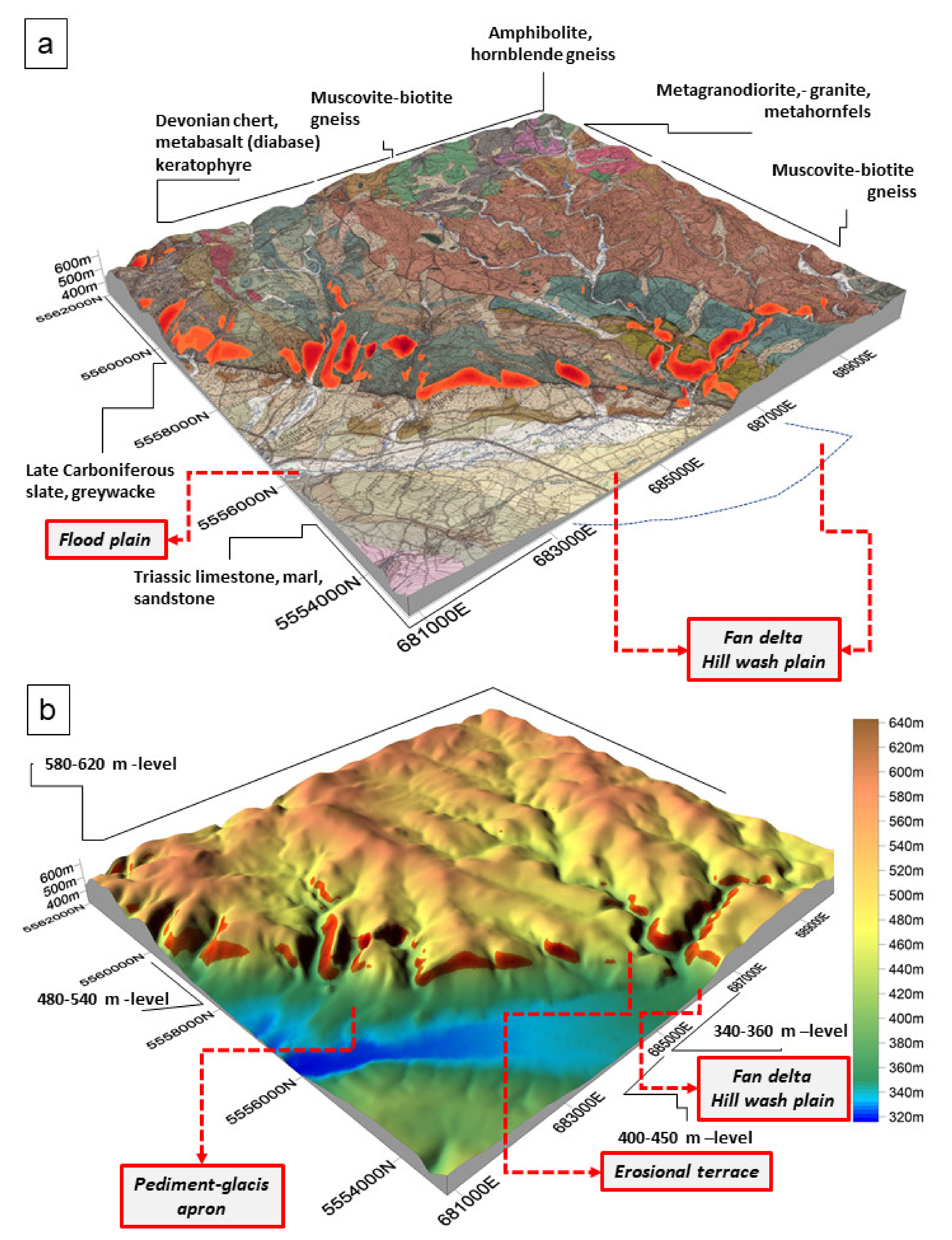
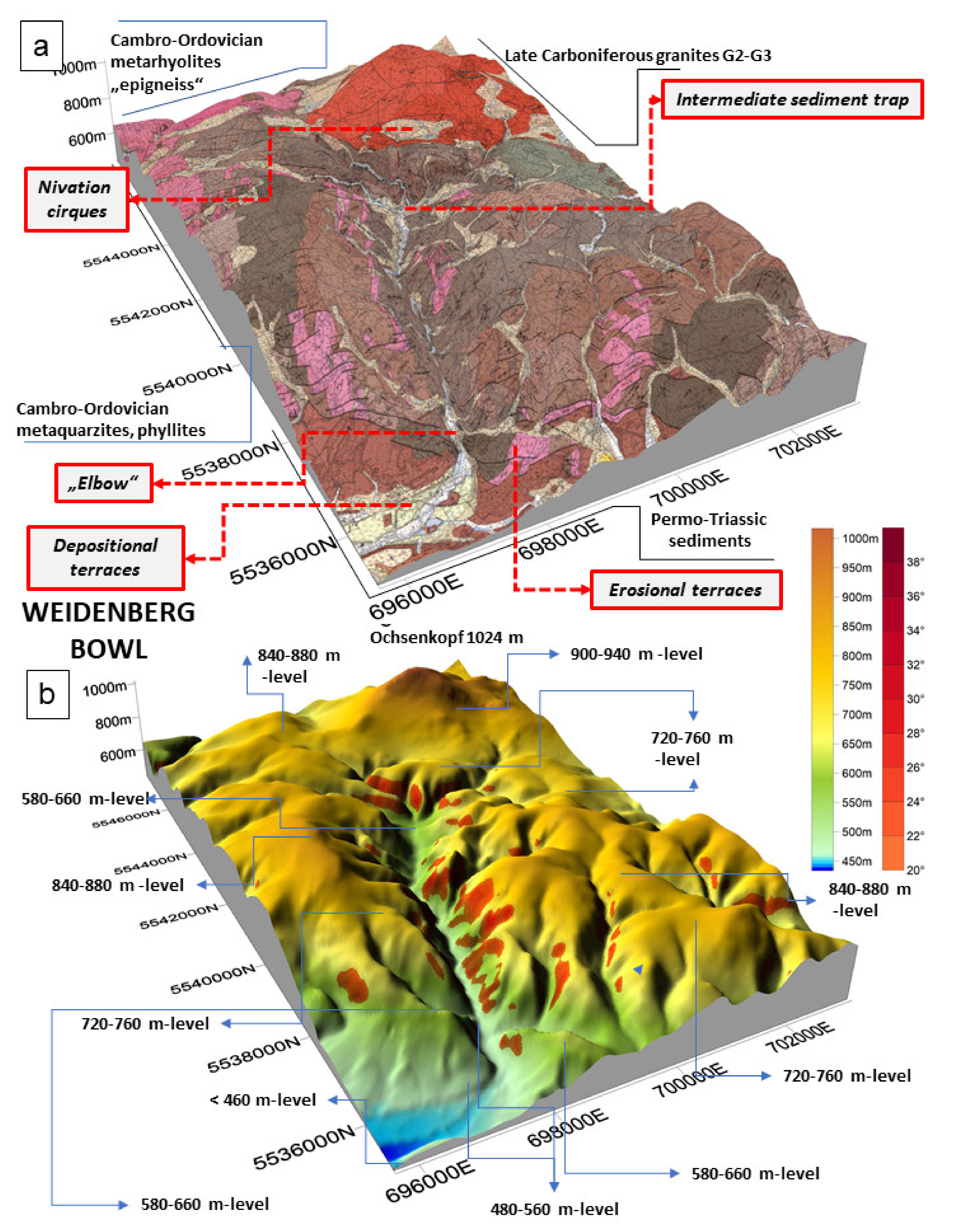
| Basement region | Franconian Slate Mts. “Frankenwald” (FW) | Fichtelgebirge Mts. “Fichtelgebirge” (FG) | Münchberg Gneiss Complex plus marginal facies “Münchberg Gneismasse” (MGC) | |
| Basement lithology | Slate, black slate (“alum shale”), greywacke, sandstone, quartzite, conglomerate, bright/black chert (proximal see DA), metabasalt (diabase), keratophyre, limestone, lamprophyre | Syeno-/monzogranite, meta-rhyolites (“epi-gneiss”), quartz (+hematite) dike rocks, dolerites, band and massive metaquartzites, phyllites | Biotite-muscovite gneiss, amphibolite, hornblende, calcsilicates, gneiss, serpentinite, eclogite, metagranodiorites/-granite-hornfels (orthogneiss), phyllite, prasinite, talc schists | |
| Foreland | Foreland lithology (detrital matter proximal—see DA) | Black chert (“lydite”), diabase, quartzite, greywacke, slates, siliceous conglomerate | Phyllite, banded meta quartzite, quartz dike rocks, massive and porphyritic epi-gneiss, porphyritic volcanites, syeno-/monzogranite, Early Triassic sandstone and carnelian | Black chert (“lydite”), diabase, prasinite, amphibolite, muscovite gneiss, orthogneiss, Late Triassic sandstone |
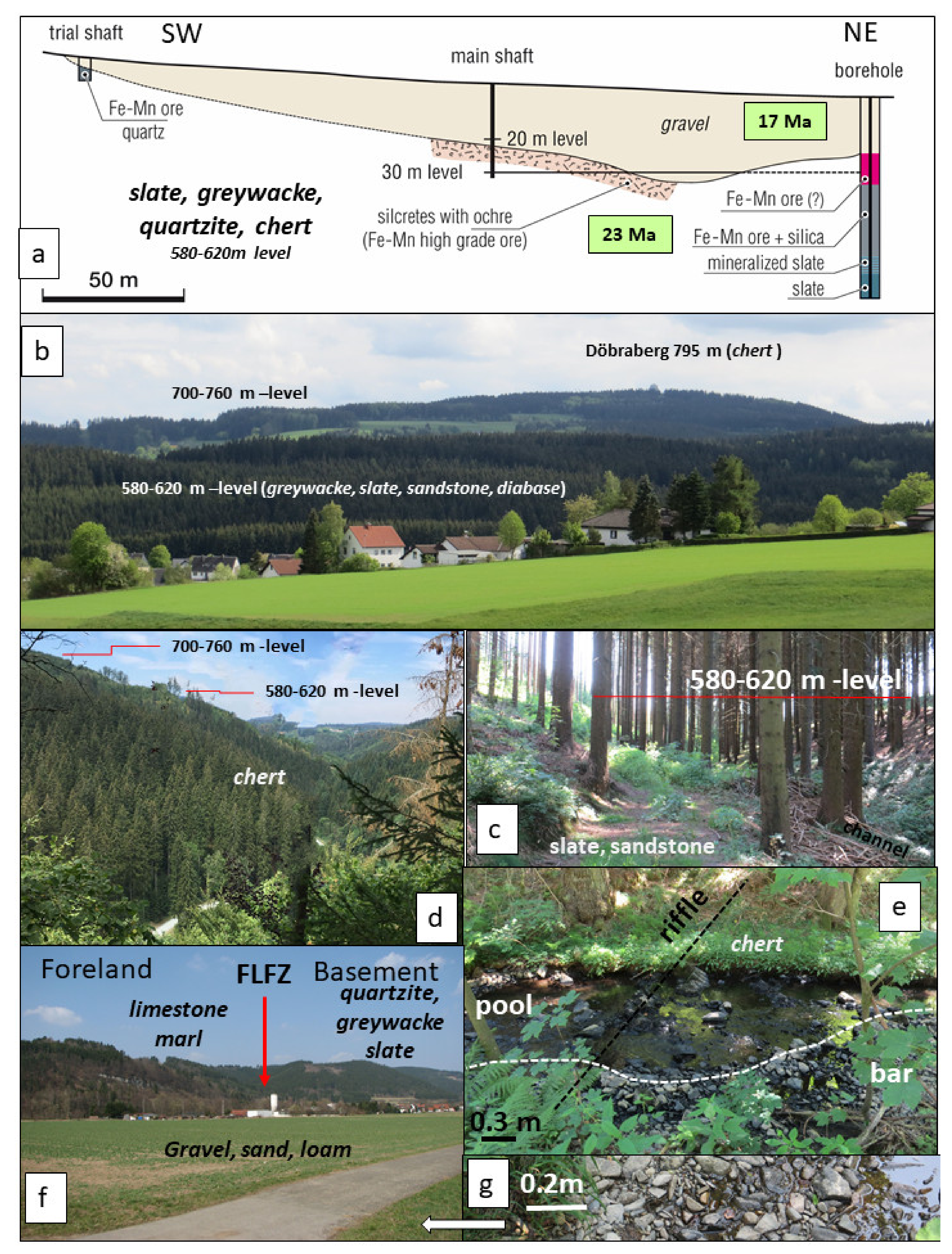
| Topography | Uppermost paleosurface (meter a.m.s.l.) | 760 (max. height Döbraberg 795—chert) | 940 (max. height Schneeberg 1052—monzogranite) | 620 (max. height Weißenstein 668—eclogite, eclogite amphibolite, pegmatoid) |
| Lower most floodplain (meter a.m.s.l.) | 340 | 400 | 355 | |
| Landform Series according to Summerfield (1991) [36] | Fluvial processes | CA: Relic large-and-shallow valleys/peneplain, straight to low sinuosity stream, single channels, non-alluvial to alluvial TA: Straight to high-sinuosity streams, flood plains. V-shaped in the upper reaches, U-shaped in the lower reaches, intermediate sediment trap Pools, riffles, steps DA: Low-sinuosity to strongly meandering stream with wide floodplain and stacked pattern of terraces within the basement and foreland, alluvial fans | CA: Straight to low-sinuosity streams, multiple channels, alluvial > (non-alluvial), dentritic pattern cascades, step-pool TA: Straight to low-sinuosity streams, intermediate sediment traps, pools, riffles, steps DA: High-sinuosity to moderately meandering stream with wide floodplains | CA: Relic large-and-shallow valleys/peneplain, low- to high sinuosity streams, single channels, alluvial drainage systems TA: Straight to low sinuosity muddy streams, Pools, riffles, steps DA: Low- to high-sinuosity streams within the foreland, hill wash plain, pediments (fluvial part/confined flow) |
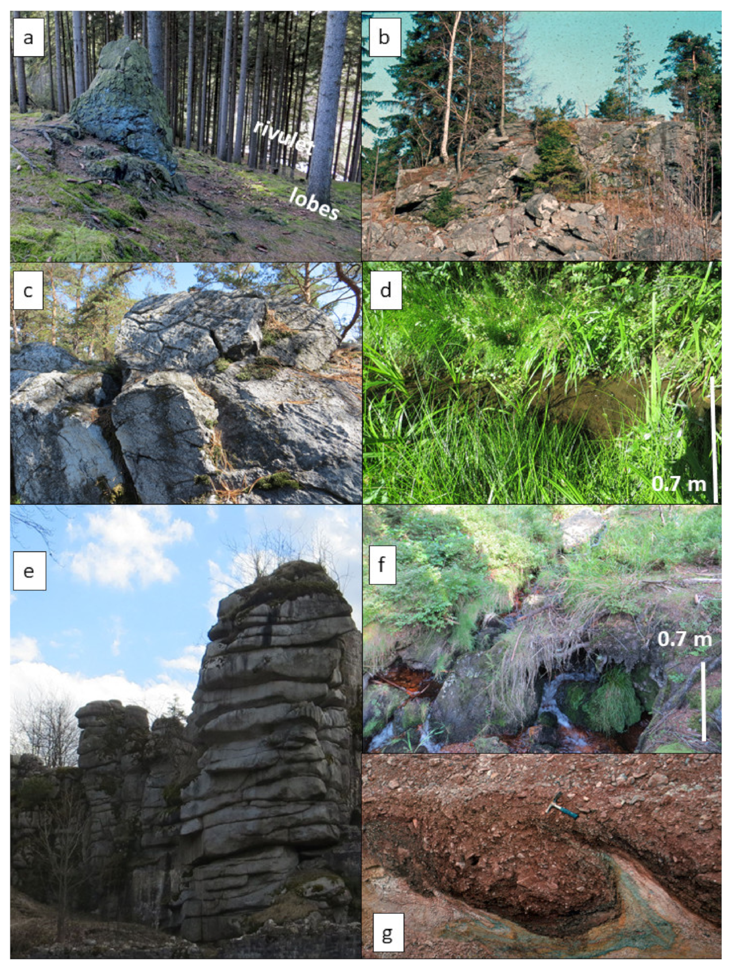
| Mass wasting processes | CA: Forested mountains with rounded tops, rare exposure of bare rocks of chert, quartzite, greywacke, sandstone talus and soil creep, TA: Solifluction, talus and soil creep DA: Solifluction | CA: Forested mountains with tors and boulder strewn tops and slopes with block streams TA: Solifluction, talus and soil creep, debris flow DA: Solifluction, talus and soil creep, debris flow | CA: Forested hills and mountains with palisades and boulder strewn tops and slopes (blockfield, block streams), monadnocks rare (metabasic to metaultrabasic rocks) TA: Solifluction, talus and soil creep, debris flow DA: pediments (colluvial part/unconfined flow) | |
| Cryogenic processes | DA: Ice wedge-cryoturbation | CA: cryoturbation, nivation cirques DA: Dragged and distorted pocket fills underneath terraces-cryoturbation | CA: cryoturbation | |
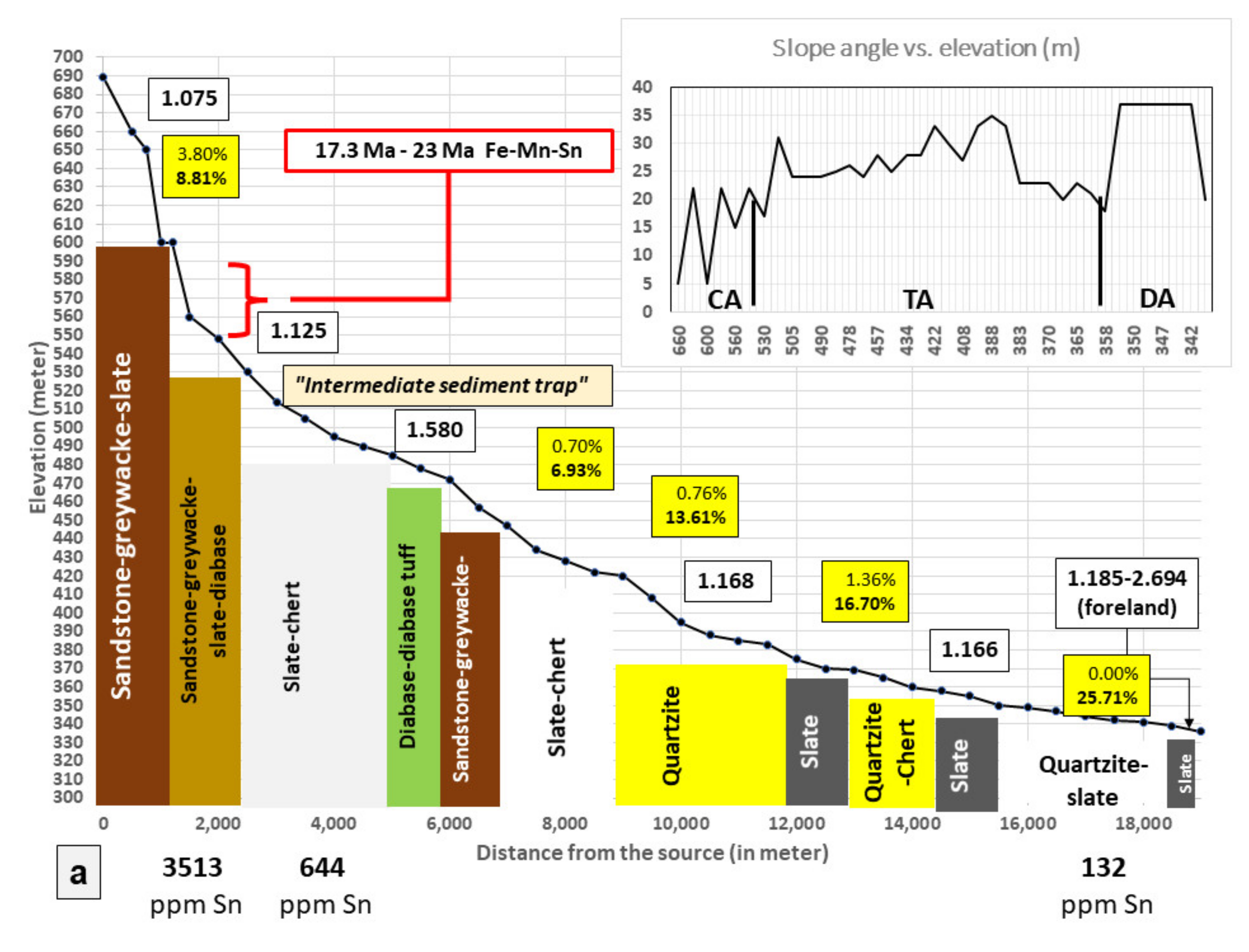
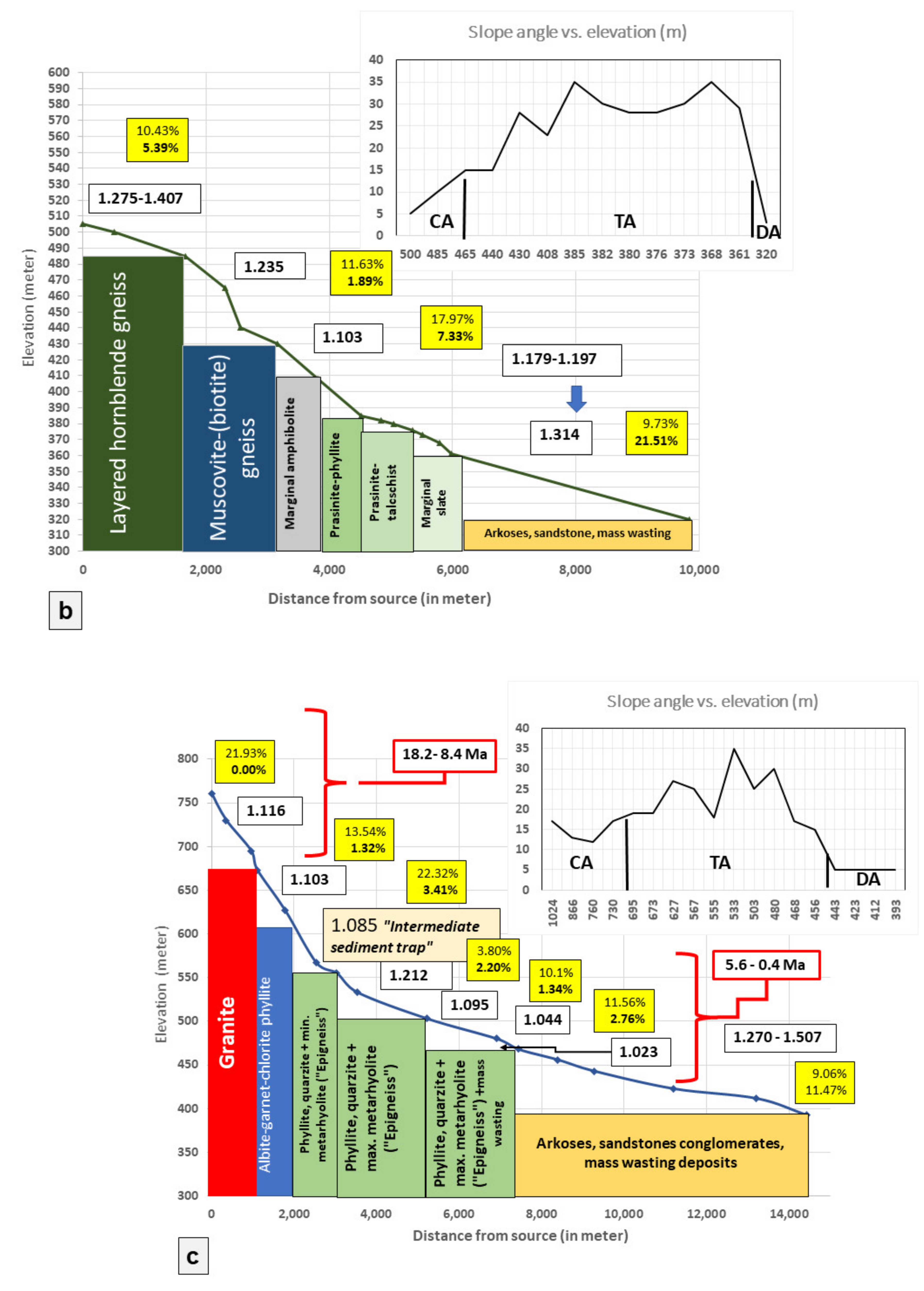
| Quantification of fluvial and colluvial deposits | Fluvial deposits (%) | CA: 8.81 TA: 6.93 to13.61 DA:16.70 to 25.71 | CA: 0.0 to 1.32 TA: 1.34 to 3.41 DA: 2.76–11.41 | CA: 5.39 TA: 1.89 DA: 7.33–21.51 |
| Mass wasting deposits (%) | CA: 3.80 TA: 0.70 to 0.76 DA: 0.0 to 1.36 | CA: 13.54 to 21.93 TA: 3.80 to 22.32 DA: 9.06 to 11.56 | CA: 10.43 TA: 11.63 DA: 9.73 to 17.97 | |
| Mineralogy of supergene alteration | Argillitization zone | CA: Regolith: illite, illite-chlorite-vermiculite mixed-layer, vermiculite, kaolinite, chlorite | CA: Regolith: kaolinite (common), smectite, vermiculite, nontronite, illite, chlorite (mainly on granite), | CA: Regolith: kaolinite (common), illite, chlorite, talc, serpentine, vermiculite (only on metabasic and ultrabasic bedrocks) |
| Duricrusts/ore-cretes | CA: Fe-Mn orecretes: cryptomelane, psilomelane, todorokite, lithiophorite, rare gibbsite, goethite, “manganomelane” Silcretes: silica Phoscretes: apatite, Al-Fe phosphate | CA: U orecretes Silcretes (uraniferous) Phoscretes (uraniferous) DA: ferricretes | CA: ± ferricretes (“limonite”) | |
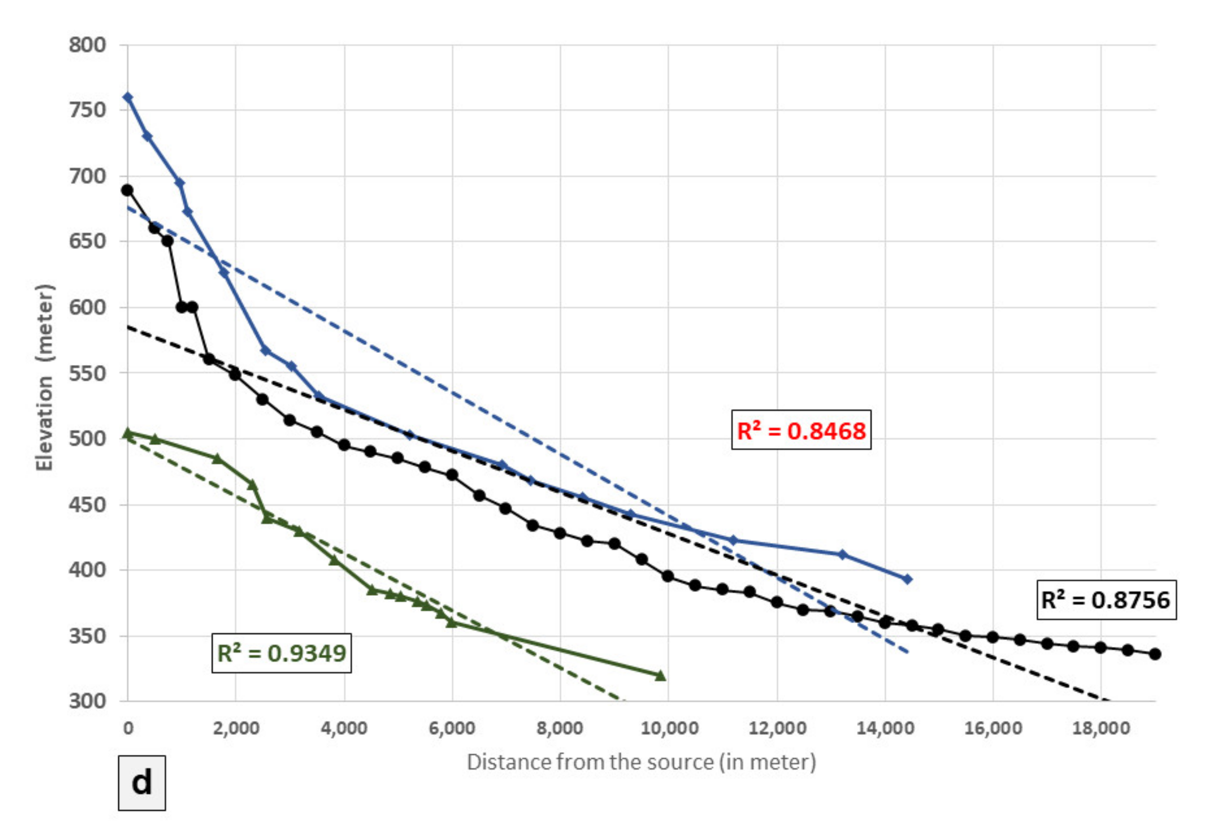
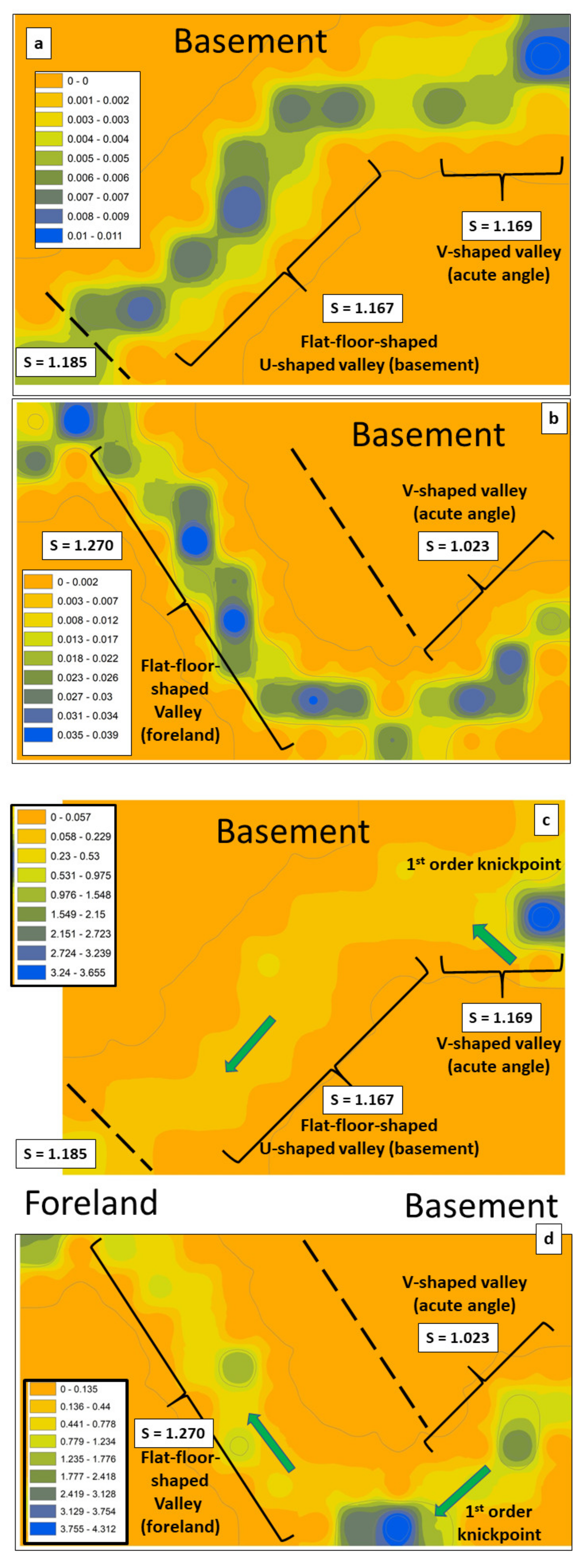
| Hydrography | Degree of sinuosity as a function of river facies | CA: 1.0748 TA: 1.1251 to 1.5802 DA: 1.1668 to 2.6938 (basement + foreland) | CA: 1.1157 TA: 1.0229 to 1.2118 DA: 1.5069 (foreland) | CA: 1.2754 to 1.4066 TA: 1.1029 to 1.2351 DA: 1.1789 to 1.3143 (foreland) |
| Slope angle as a function of river facies | CA: 5–22° TA: 17–37° CA: 5–36° (basement + foreland) | CA: 12–19° TA: 10–35° DA: 5–10° | CA: 5–15° TA: 16–35° DA: 5–13° | |
| Orientation relative to bedrock structures + fluvial pattern and channel morphology | Single-channel to antler-shaped See Table 2 | Dentritic to parallel See Table 2 | Dentritic to antler-shaped See Table 2 | |
| Sediment Petrography | Grain size distribution (%) | Clay + silt: 12.2 Sand: 14.9 Pebble:38.9 Cobble + boulder: 34.0 | Clay + silt: 11.4 Sand: 6.2 Pebble: 2.8 Cobble + boulder: 79.6 | Clay + silt: 56.6 Sand: 12.3 Pebble: 15.2 Cobble + boulder: 15.9 |
| Grain morphology | See Table 3b | See Table 3a | See Table 3a | |
| Grain orientation (“situmetry”) | See Table 3b | See Table 3a | See Table 3a | |
| Site | Gravel (%) | Height (m) | Age Dating | Interpretation (Current Study) |
|---|---|---|---|---|
| Steinach “Terrace T4” | Epigneiss 20, phyllite 60, quartz, quartz 10, quartzite 10 | >480 | Middle Pleistocene | Alluvial and colluvial sediments on the low scarp mixed with relic fluvial deposits (unconfined flow and creep) |
| Steinach “Terrace T3” | Epigneiss 6, phyllite, 18, quartz 70, quartzite 6 | 480 | Middle Pleistocene | Fluvial terrace |
| Steinach “Terrace T2” | Epigneiss 10, phyllite 80, quartzite 9 Quartz + granite 1 | 460 | Middle to Late Pleistocene | Fluvial terrace |
| Steinach “Terrace T1” | Epigneiss 6, phyllite 75, quartzite 12, quartz 5, granite 1 | 440 | Late Pleistocene to Early Holocene | Fluvial terrace |
| Recent floodplains “T0” | Epigneiss 12, phyllite 70, quartzite 12, quartz 6 | 400–420 | Holocene | Floodplain |
| Stages | VLG-Type | LGG-Type | LHG-Type | Climate | Age |
|---|---|---|---|---|---|
| Forming the lithological and structural (folding + faulting) framework for the SSS | Very-Low Grade metamorphic basement | Low-Grade metamorphic basement intruded by Granites | Low/medium-to High-Grade metamorphic basement | Variable climate regimes | Late Paleozoic Variscan Orogeny |
| Forming the structural framework (faulting) for the SSS | Strong faulting, uplift and erosion of topstrata | Strong faulting, updoming, uplift and erosion of topstrata | Strong faulting, uplift and erosion of topstrata | Variable climate regimes | Mesozoic to Paleogene |
| Tectonic Event (Driver I) | Fracturing, uplift, tilting of the paleosurface as a consequence of the NE-SW striking Eger- Graben Rift. Tectonically- related formation of the prestage drainage systems Forming the blue print” of the SSS | Late Oligocene to Middle Miocene 29–19 Ma | |||
| Prestage- Fluvial-alluvial-(lacustrine) Paleo-landscape | Wide and shallow valleys braided to meandering rivers/ coarse-gr. deposits Sinuosity > 2.5 | Wide and shallow valleys braided to meandering rivers/ coarse-gr. deposits Sinuosity > 2.5 | Wide and shallow valleys braided to meandering rivers/ coarse-gr. deposits Sinuosity > 2.5 | Humid tropical to subtropical wet and dry climate | Early- to Middle Miocene 23–14 Ma |
| Prestage Fluvial paleo-landscape | Regolitisation, etch planation, formation of inselbergs in the basement, trunk rivers in the foreland (e.g., Main, Rhein.) | Regolitisation, etch planation, formation of inselbergs in the basement, trunk rivers in the foreland (e.g., Main, Rhein.) | Regolitisation, etch planation, formation of inselbergs in the basement, trunk rivers in the foreland (e.g., Main, Rhein.) | subtropical wet and dry climate | Middle to Late Miocene 8.4–5.6 Ma |
| Tectonic Event (Driver II) | Fracturing, uplift in the South German Block and reactivation of the NW-SE striking FLFZ accompanied by a rising gradient Starting drainage and accelerating incision of the SSS | Middle Miocene to Plio-Pleistocene 15.3–2.3 Ma | |||
| Proto-Straight to low sinuosity drainage system (SSS) (CA)⇒ Modern SSS | Onset of the zone of headwaters of the SSS Sinuosity 1.075 Slope angle 5 to 22° F/M ratio: 2.323 | Formation of tors, palisades Onset of the zone of headwaters of the SSS Sinuosity 1.116 Slope angle 2 to 18° F/M ratio: 0.062 | Formation of tors, palisades Onset of the zone of headwaters of the SSS Sinuosity 1.275–1.407 Slope angle 5 to 15° F/M ratio: 0.517 | subtropical climate drier regime | Pliocene to Early Pleistocene 4.0–1.8 Ma |
| Modern SSS (TA) | Incision of V-shaped wide-angle valleys Sinuosity 1.125 Slope angle 18 to 31° | Block stream Incision of V-shaped wide-angle valleys Sinuosity 1.103 Slope angle 15 to 27° | Block stream | Glacial period with cold and warmer stages | Early Pleistocene < 1.8 Ma |
| Modern SSS (TA) | Intermediate sediment traps | Intermediate sediment traps | Not developed Erosional unconformity | Glacial period with cold and longer warmer stages | |
| Modern SSS (TA) | Mass wasting landforms Incision of V-shaped acute valleys Sinuosity 1.580–1.169 Slope angle 31 to 35° KP F/M ratio: 17.908 KP | Mass wasting landforms Incision of V-shaped acute Sinuosity 1.212–1.023 Slope angle 27 to 35° F/M ratio: 0.153 | Mass wasting landforms Incision of V-shaped acute Sinuosity 1.235–1.103 Slope angle 24 to 35° F/M ratio: 0.163 | Glacial period with cold and warmer stages | 0.4 Ma Middle Pleistocene |
| Modern SSS (TA) | Mass wasting landforms Flat-floor-shaped/ U-shaped valley Sinuosity 1.167 Slope angle 19 to 35° | Not developed | Not developed KP | Glacial period to postglacial warm temperate | Holocene |
| Modern SSS (DA) | Mass wasting landforms Fluvial depositional terrace (T4) Slope angle < 20° | Mass wasting landforms Fluvial depositional terrace (T4) Slope angle < 5° | Glacial period with cold and warmer stages | 0.4 Ma Middle Pleistocene | |
| Modern SSS (DA) | Fluvial depositional terrace (T3) | Fluvial depositional terrace (T3) | |||
| Modern SSS (DA) | Fluvial depositional terrace (T2) | Fluvial depositional terrace (T2) | Middle to Late Pleistocene | ||
| Modern SSS (DA) | Cryogenic landforms Fluvial depositional terrace (T1) Sinuosity 1.185 F/M ratio: 18.904 | Cryogenic landforms Fluvial depositional terrace (T1) Sinuosity 1.270 KP F/M ratio: 0.987 KP | Hillwash plain (T1) Sinuosity 1.197 Slope angle < 5° F/M ratio: 1.197 | Glacial period with cold and warmer stages | Late Pleistocene to Early Holocene |
| Modern SSS (DA) | Floodplain (T0) Sinuosity 2.694 | Floodplain (T0) Sinuosity 1.507 | Floodplain (T0) 1.314 | Postglacial moderate humid temperate | Holocene |
| The Geomorphological-Geodynamic Maturity Stages | Maturity | ||
|---|---|---|---|
| Pre-Mature | Mature | Super-Mature | |
| Geodynamic setting | Moderately eroded and active mountain belts of Late Mesozoic to Cenozoic age (e.g., Andes) + island arcs | Highly eroded mountain belts of Paleozoic and Early Mesozoic age (e.g., Hercynian/Variscan Mountain Ridges) + continental grabens | Deeply eroded cratons of Precambrian age (e.g., Guyana Shield) + continental grabens + island arcs |
| Occurrence of weathering (see Figure 15) | Absent (only slightly altered parent material) moderate argillitization | Argillitization >> duricrusts | Duricrusts—argillitization |
Publisher’s Note: MDPI stays neutral with regard to jurisdictional claims in published maps and institutional affiliations. |
© 2021 by the authors. Licensee MDPI, Basel, Switzerland. This article is an open access article distributed under the terms and conditions of the Creative Commons Attribution (CC BY) license (https://creativecommons.org/licenses/by/4.0/).
Share and Cite
Dill, H.G.; Buzatu, A.; Balaban, S.-I. Straight to Low-Sinuosity Drainage Systems in a Variscan-Type Orogen—Constraints from Tectonics, Lithology and Climate. Minerals 2021, 11, 933. https://doi.org/10.3390/min11090933
Dill HG, Buzatu A, Balaban S-I. Straight to Low-Sinuosity Drainage Systems in a Variscan-Type Orogen—Constraints from Tectonics, Lithology and Climate. Minerals. 2021; 11(9):933. https://doi.org/10.3390/min11090933
Chicago/Turabian StyleDill, Harald G., Andrei Buzatu, and Sorin-Ionut Balaban. 2021. "Straight to Low-Sinuosity Drainage Systems in a Variscan-Type Orogen—Constraints from Tectonics, Lithology and Climate" Minerals 11, no. 9: 933. https://doi.org/10.3390/min11090933
APA StyleDill, H. G., Buzatu, A., & Balaban, S.-I. (2021). Straight to Low-Sinuosity Drainage Systems in a Variscan-Type Orogen—Constraints from Tectonics, Lithology and Climate. Minerals, 11(9), 933. https://doi.org/10.3390/min11090933