Research on Automatic Construction Method of Three-Dimensional Complex Fault Model

Abstract

Three-dimensional complex fault modeling is an important research topic in three-dimensional geological structure modeling. The automatic construction of complex fault models has research significance and application value for basic geological theories, as well as engineering fields such as geological engineering, resource exploration, and digital mines. Complex fault structures, especially complex fault networks with multilevel branches, still require a large amount of manual participation in the characterization of fault transfer relationships. This paper proposes an automatic construction method for a three-dimensional complex fault model, including the generation and optimization of fault surfaces, automatic determination of the contact relationship between fault surfaces, and recording of the model. This method realizes the automatic construction of a three-dimensional complex fault model, reduces the manual interaction in model construction, improves the automation of fault model construction, and saves manual modeling time.

1. Introduction

Fault modeling is the basis of three-dimensional (3D) geological modeling and has important value in basic geological research and various geological science and technology applications. In areas with developed faults, there are often not only a large number of faults, but also complex faults with special structures, such as X-type faults, multilevel y-type faults, etc. It is very difficult to model faults in such areas. Currently, there are two main ways to construct fault models: the explicit way and the implicit way. Explicit modeling is constructed by geologists according to their own knowledge and experience in order to adjust the model through manual interactive operations, and the result is subject to the cognition of a modeler [1,2,3]. Implicit modeling adopts the mathematical solution method of scalar fields, but it requires the setting of boundary conditions and additional artificial data points to make the scheme feasible [2,4,5]. Godefroy et al. [6] and Grose et al. [7] introduced kinematics into implicit modeling and realized the parametric modeling of folds. Current implicit methods can only represent a limited number of unconformities owing to computational and storage limitations [3]. Explicit modeling can be flexible, but it is time-consuming due to numerous interactive operations. To free geologists from the complex interactive modeling work and promote the application of 3D geological modeling in related fields, the automatic construction of 3D complex fault models has become a major issue.

The construction of the fault model mainly includes four steps: data preparation, fault surface generation, fault-fault contact relationship processing, and model recording. In addition to the geological survey data, the data required for modeling often uses seismic data, logging data, and remote sensing images. These data are geologically interpreted to obtain geometric data such as points and lines that meet the requirements as input data for modeling [8,9]. Jessell et al. [10] realized the automatic deconstruction of geological maps and the automatic definition of fault contact relations; Wu, X. et al. [11,12] and Qi et al. [13] realized automatic fault interpretation of seismic data. As for the 3D fault surface, automatic generation and visualization technology has been relatively mature. The current mainstream method uses a triangular mesh model to finely describe the detailed characteristics of the fault surface [14,15]. The pillar grid and stair-step grid can also describe fault surfaces, but they will simplify the surface characteristics and reduce the model accuracy to improve the efficiency of numerical simulation [16,17,18,19,20]. Exploring and realizing the automatic processing of the fault-fault contact relationship are key issues for the automatic construction of 3D complex fault models. The processing of the fault-fault contact relationship includes the determination of the intersection station, the major or minor fault, the termination of fault surfaces, and the truncation of the minor fault. Although the judgment of intersection has been automated, the determination of the major or minor fault, the processing of fault surface termination, and the truncation of minor faults still require manual interaction [21,22,23]. The determined result of the fault-fault contact relationship is mainly recorded by the key pillar, matrix, and binary tree methods. The pillar-based fault model uses a special pillar that is manually added to mark the intersection of fault surfaces, but it cannot handle multilevel branch faults. The matrix method can completely record the contact relationship of each fault, but it is not easy to edit intuitively with high information redundancy and high dependence on manual participation [24]. The fusion fault block method extends fault surfaces to divide the geological body into fault blocks and organizes the fault-fault contact relationships in the form of a binary tree, which can construct multilevel y-shaped faults [25,26]. However, the truncation operation still requires manual participation, and the accuracy of the model needs to be improved [27].

This study provides a new solution for the automatic processing of the fault-fault contact relationship of the complex fault model. Multisource data (seismic data, logging data, remote sensing images, etc.) were interpreted as labeled fault point data, and the knowledge of geologists was converted into point data that can be easily recognized by the computer through labels. With the labeled datasets, the modeler can automatically construct the same complex fault truncation model. Therefore, the shortcomings of explicit modeling, which are not easy to reproduce, can be fixed. The specific modeling process will be described in Section 2. The methods of model construction, minor fault truncation, and model recording are described in Section 3. After constructing a fine triangulation fault surface model with the fault point data, the intersecting relationship of the fault surfaces is automatically judged and recorded by the graph model of graph theory. Graph theory has some applications in the field of geology (such as fracture modeling [28,29,30], two-dimensional (2D) geological map recognition [10], the organization of geological relations [31,32], etc.). Compared with the fault model, the fracture model has a small scale and a simple surface structure. The application of the graph model in these two problems is also different. In the fracture network, the edges of the graph model represent the fracture surfaces, and the vertices represent the intersection points of the fracture surfaces. For large-scale objects such as faults, graph theory has more applications. For instance, in the recognition of 2D geological maps, the vertices and edges correspond to geometric points and edges [10,30]. In uncertainty modeling, the vertices represent the fault interpretation points, and the edges represent that the two fault points belong to the same fault [33]. In this study, each vertex represents a fault surface, and the edges represent the intersection relationship of the fault surfaces. The major and minor type of the intersecting faults are automatically updated according to the attributes of graph theory. Further, the minor faults are automatically truncated according to the truncation standard. The final result of the fault model is recorded in extensive markup language (XML), which not only makes it easy to analyze the structure of the fault-fault contact relationship, but also makes it easy to modify the type of major or minor fault. In short, the method in this study reduces the manual interaction in model construction, improves the automation of fault model construction, and saves manual modeling time.

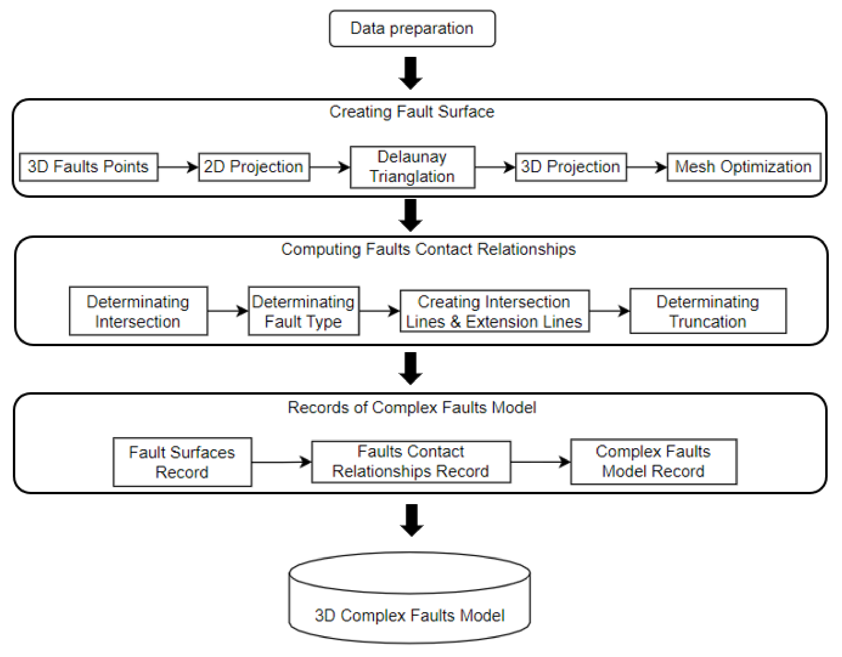
2. Automatic Construction Process of Complex Fault Model

The automatic construction of a 3D complex fault model includes three steps: the construction of the 3D fault surface model, the calculation of the fault contact relationship, and the description of the complex fault model (Figure 1). The contact relationship of faults is automatically calculated, the truncated fault model is automatically generated, and the results of the fault model construction can be reused after recording.

2.1. Data Preparation

Multisource data can be interpreted into fault point data, fault sticks, and fault polygons. If there are enough fault point data, fault sticks and fault polygons can be transported to a pointset. Therefore, the fault data in this paper were interpreted as labeled fault point data. Fault points belonging to the same fault have the same label. To avoid the misunderstanding of truncation, fault point data on two sides of one fault will be marked with different labels.

2.2. 3D Fault Surface Model Construction

The triangulation method of the two-dimensional plane is very mature [12], so the 3D fault point data are first projected to the two-dimensional (2D) plane (a least squares fitting plane illustrated by Figure 2) one by one and triangulated to generate a 2D triangulation plane. Then, according to the mapping rules, the two-dimensional triangulation model is mapped onto a 3D triangulated surface mesh, and mesh optimization is performed to finely describe the fault surface shape.

2.3. Determination of Fault-Fault Contact Relationship

The contact relationship of fault surfaces includes disjoint (Figure 3a) and intersecting relationships, in which an intersecting relationship contains intersection stopping (Figure 3b) and intersection cutting (Figure 3c). To determine the fault-fault contact relationships, it is necessary to determine whether the faults intersect first. There is a threshold about fault-fault distance between two disjoint faults. If the distance is within the threshold, one fault’s surface will be extended to make an intersection as shown in Figure 3b [34], and the contact relationship is deemed to be intersection stopping. According to recorded intersection status, the intersection line of the two intersecting faults is calculated. The location of the intersection line on the fault surface will decide whether to extend the intersection line to truncate one of the fault surfaces (details in Section 3.2).

2.4. Recording of Complex Fault Model

Graph theory was utilized in this paper to record complex fault models. The vertices represent the fault surface models, and the edges represent the contact relationship of two fault models. If there is an edge between two vertices, it means that the fault surfaces represented by these two vertices intersect. The XML can flexibly record the graph structure [35], and it is convenient to give abundant information to the elements in the graph. The XML can also describe the complex fault model and record its information, which includes details regarding the fault surface and the fault contact relationship. The output of the model result will be a triangular mesh and graph network about fault-fault contact relationships.

3. Automatic Construction Method of Complex Fault Model

At present, the construction of complex fault models, especially when calculating the complex contact relationships of faults, requires significant manual participation. The key point in realizing the automatic construction of complex fault models is to allow the computer to automatically calculate the fault contact relationship and determine the truncation form. This paper proposes a set of complex fault model construction methods based on triangulation network fault surfaces, including (1) the automatic generation method of fault surfaces, (2) the automatic calculation method of fault contact relationships, and (3) complex fault model recording methods.

3.1. Automatic Generation Method of Fault Surface

The automatic construction process of the 3D fault surface model is as follows (Figure 4):

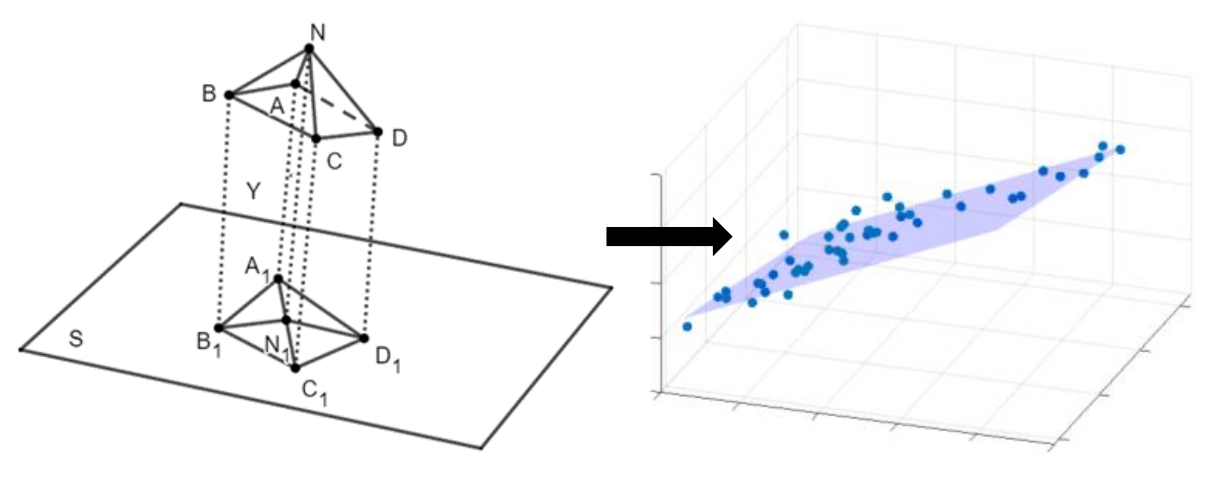
• Calculate the centroid coordinates and 2D fitting plane normal vector $(w_1,w_2,w_3)$ of the 3D fault point dataset. The plane equation ($S:w_{1}x+w_{2}y+w_{3}z+w_4=0$) can be calculated according to the centroid coordinates and normal vector. Project the 3D points’ set to the 2D surface one by one and perform triangulation to generate a 2D triangular mesh surface.
• Based on the one-to-one correspondence between the points in the 3D space and the 2D space, the topological relationship of the two-dimensional triangulation model is mapped to the 3D space to form a 3D fault surface.
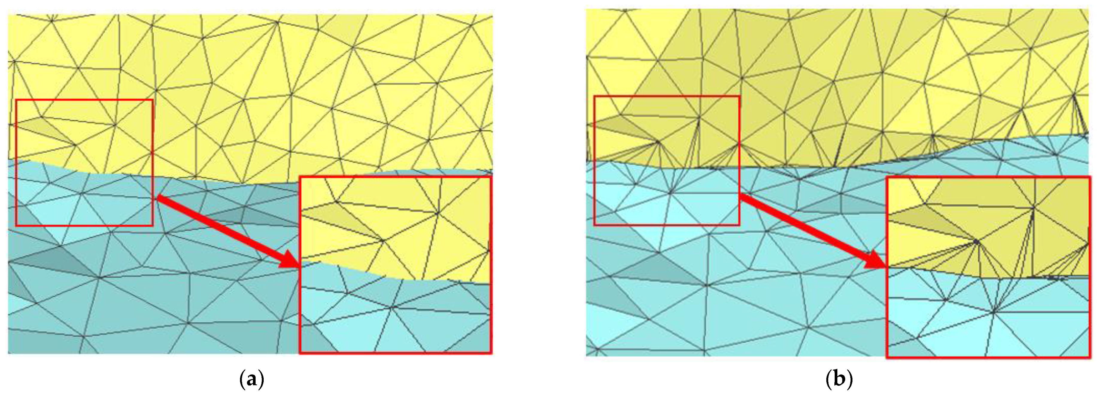
• Optimize the fault surface model, reduce the deformed triangular grid unit, and ensure the quality of the grid.

3.2. Automatic Determination Method of Fault-Fault Contact Relationship

The two intersecting faults are called major and minor faults, respectively. The major fault will not be truncated, whereas if the minor fault needs to be truncated, further judgment is required [21]. The automatic determination of the fault-fault contact relationship first needs to determine whether the fault surfaces intersect. Two faults that have a distance within the threshold, as discussed in Section 2.2, will also be regarded as intersecting surfaces. After determination of the intersection, a complex fault model is generated according to the following process (Figure 5): (1) determine the type of the fault (major/minor fault); (2) calculate the intersection line (and its extension line) of the fault surface; (3) update the fault surface grid model and its topological relationship using the ear clipping algorithm; and (4) truncate the minor fault surface and generate a complex fault model.

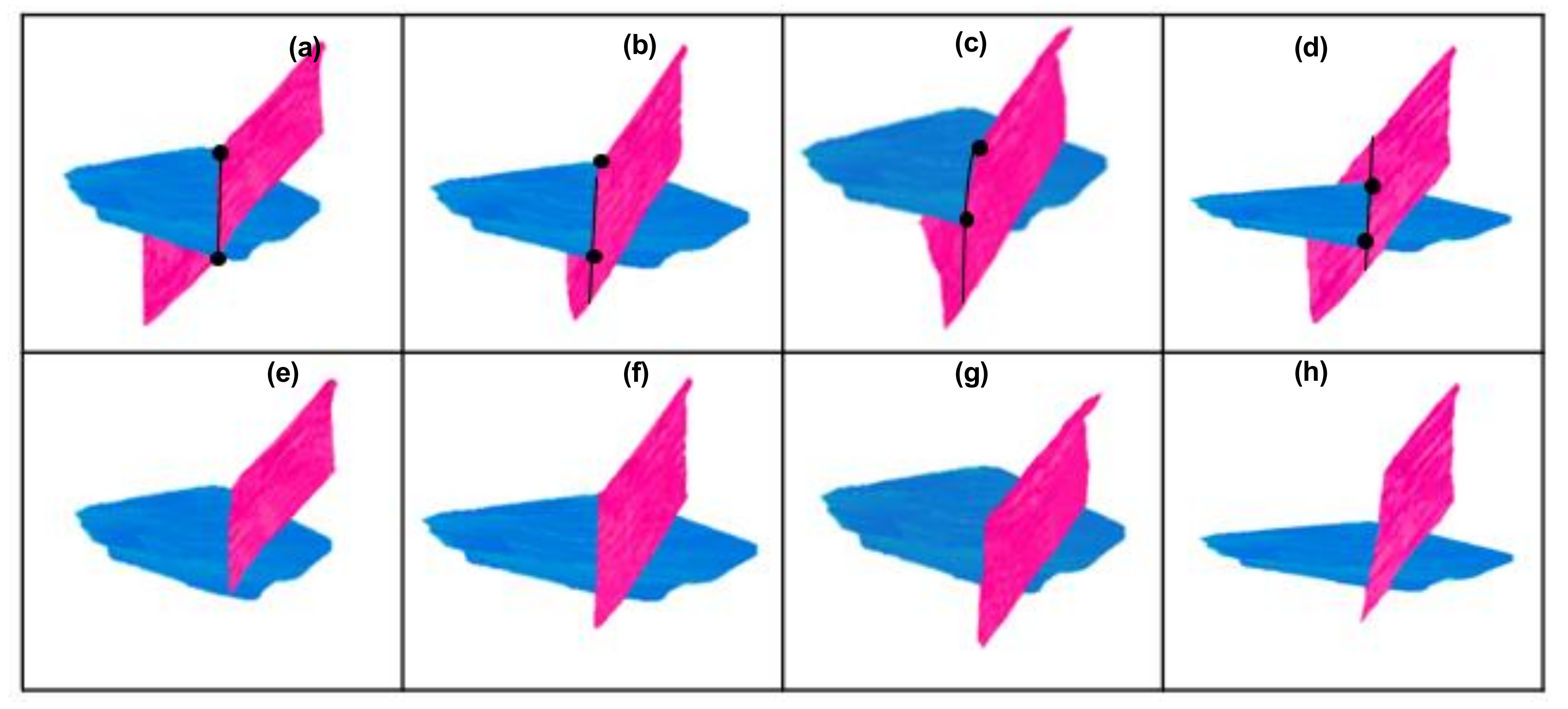
3.2.1. Determining the Type of the Fault

The first basis for determining whether the fault is a major or minor fault is the formation time of the fault, and the major fault has a later formation time than the minor fault does. Abbott et al. used geometric elements as the basis for judging the major and minor faults, such as the number of fault points, the degree of extension of the fault surface, and the number of fault points on both sides of the intersection line of the fault surface [21]. In the simple case where two faults intersect, geometric elements are feasible as a basis, but, for multilevel complex fault models, this method cannot be used to make effective judgments. In addition, the number of faults associated with a certain fault should also be considered to ensure that the faults in the model are as interconnected as possible.

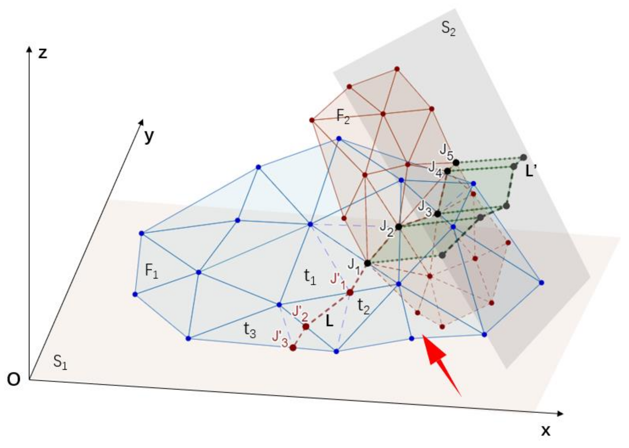
3.2.2. Calculation of Intersection & Extension Line of Fault Surface

The intersection line of the intersecting fault surface is formed by the intersection point produced by the intersection of the triangular patches. The intersection line of the two intersecting fault surfaces was calculated according to the following steps:

• Record the intersecting triangle patches in each fault surface.
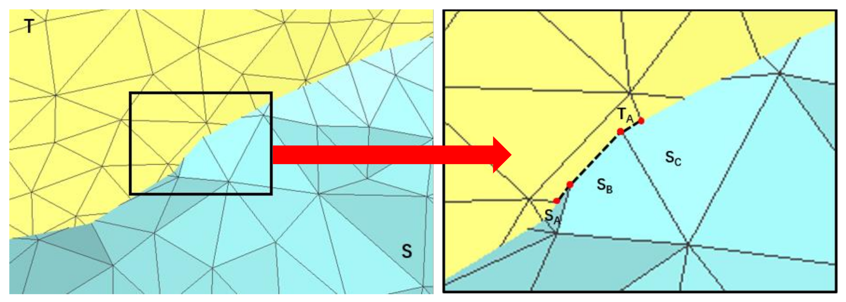
• Select one of the fault surfaces and calculate the intersection points on each triangle plane recorded in Step 1. One triangular patch may intersect with multiple triangular patches, resulting in multiple intersection points (Figure 6).
• Based on the topological relationship between the triangular patches, all the intersection points on the fault surface are related to generate the intersection line.

Figure 7 shows four types of fault surface intersections, in which the blue plane is the major fault and the red plane is the minor fault. The intersection line of (a) directly cuts across the minor fault surface, and the intersection lines of (b)–(d) partially cut across the minor fault surface. It is necessary to extend the intersection line to completely truncate the fault surface.

Considering two factors, the extension trend of the original intersection line and the spreading trend of the fault surface, a method for extending the intersection line of the fault surface is designed, which can fit the line to fine fault surface. The extended line divides the minor faults into two parts. The specific process is illustrated in the following example (Figure 8):

$F_1$ and $F_2$ are two intersecting fault surfaces in space, and it is known that $F_2$ is the major fault and $F_1$ is the minor fault. $S_1$ is a reference surface, which is actually the xOy plane paralleled with the horizontal plane, and $S_2$ is the parallel plane that fits the 2D plane of $F_2$. $F_1$ and $F_2$ intersect to produce intersection points to form a line segment $L\prime =\{J_1,J_2,J_3,J_4,J_5\}$, which cannot divide $F_1$ into two parts. Therefore, the intersection line needs to be extended to divide $F_1$; since the process of extension is the same on both sides of the line, the following example explains the process in detail for only one side.

Find the triangular patch $t_1$ that contains the point $J_1(x_1,y_1,z_1)$ in $F_1$ according to the geometric topological relationship and add the vertices into the point dataset of $F_2$. Calculate the new fit plane $F_2^1$:$w_{1}x+w_{2}y+w_{3}z-(w_1{x}_1+w_2{y}_1+w_3{z}_1)=0$ based on the normal vector $(w_1,w_2,w_3)$ of $F_2$ with the new point dataset and the point $J_1(x_1,y_1,z_1)$. The intersection point $J_1\prime$ will be formed by the triangular patch $t_1$ and $F_2^1$. $J_1\prime$ is a point on the extending line of the intersection. Add another three vertices of the triangular patch $t_2$ into the point set of $F_2$ and fit a new plane $F_2^2$. Calculate the normal vector $(n{w}_1,n{w}_2,n{w}_3)$ of the new plane, $F_2^2$, which can form a new plane with point $J_1\prime$. The triangular patch contains $J_1\prime$, and the new plane can create a new intersection point $J{\prime }_2$,……, and so on. Finally, the extended line is traced and generated until the edge of $F_1$. Figure 8 shows that $F_1$ is truncated into two parts by $F_2$ using the extension line segment set $L=\{J_1\prime ,J_2\prime ,J_3\prime \}$ and intersection line segment set $L\prime =\{J_1,J_2,J_3,J_4,J_5\}$. According to the rules of truncation described in Section 2.2, the right part pointed by the arrow will be removed, and the left part will be kept.

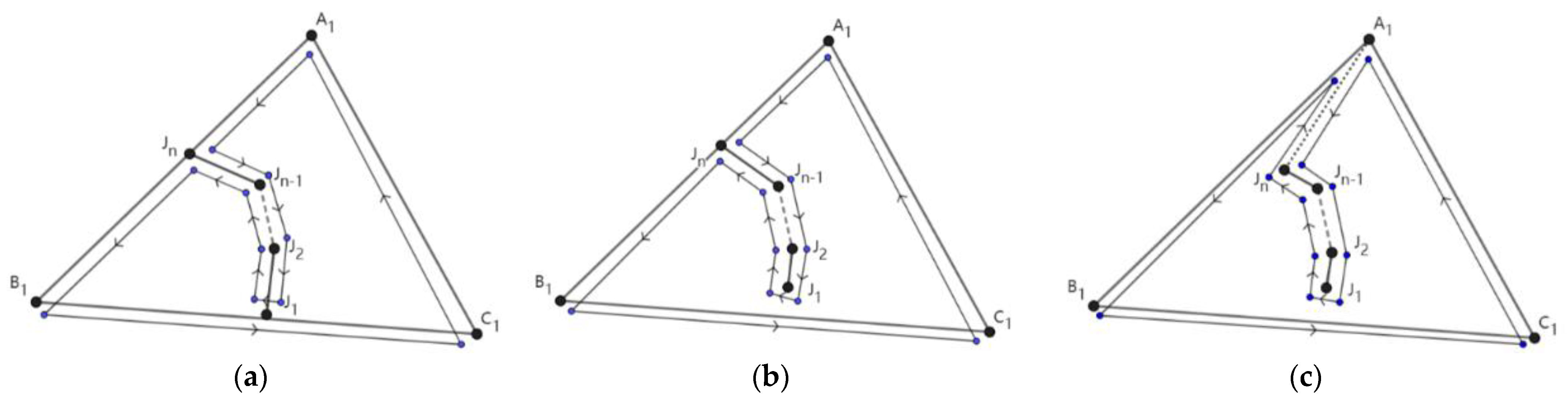
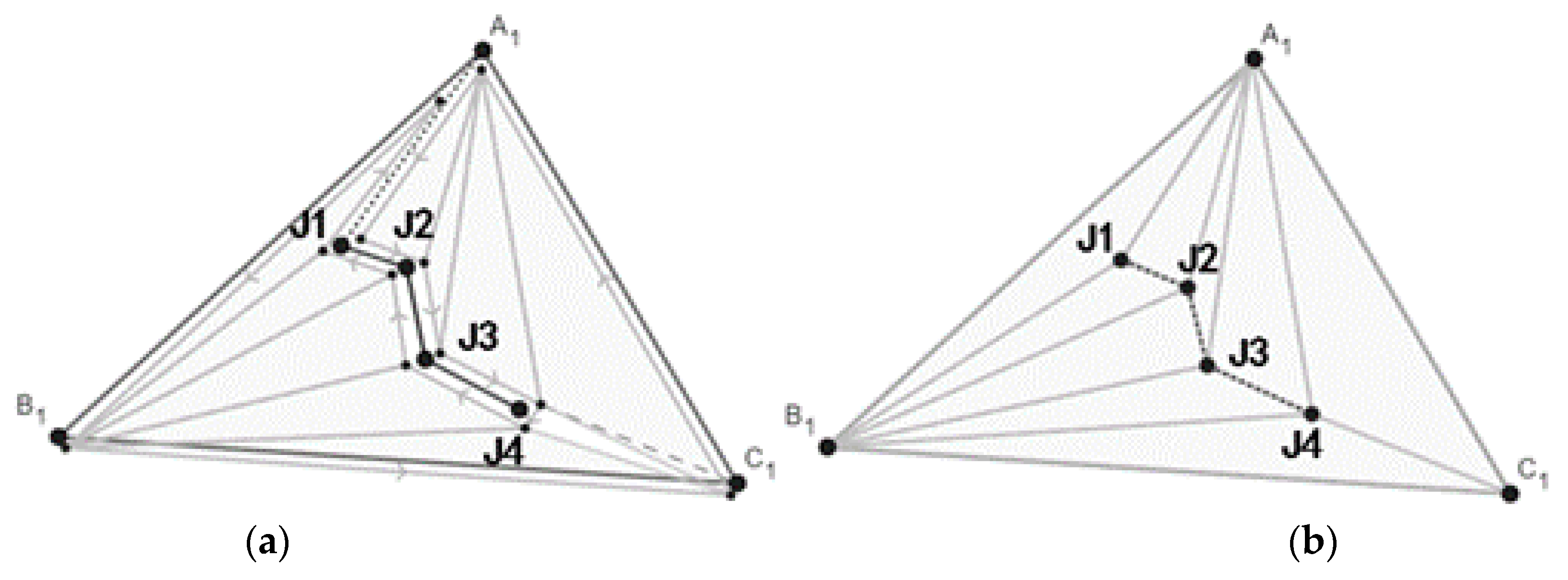
3.2.3. Updating Geometrical Topological Relations with Ear Clipping Algorithm

The fault surface is represented by a triangulated irregular net (TIN). However, the calculated intersection points of the two intersecting fault surfaces destroyed the geometrical topological structure of the original triangulation fault surface. To ensure the consistency of the fault surface data, the ear-clipping algorithm was used to triangulate the triangular patches that have the intersection and extension lines of the fault surface [36,37]. The ear-clipping algorithm includes two steps: building a closed polygon with a triangle and segmenting the triangle. For triangles with intersections, a closed polygon is constructed with intersections and triangle vertices sorted based on the coordinates. The polygon is divided into multiple triangles, and the topology of the fault surface is updated.

Two fault surfaces intersect where a triangle $t(A_1{B}_1{C}_1)$ on a certain fault surface and a triangle on another fault surface produce intersection points. The sorted intersection points constitute a set, $J=\{J_1,J_2,\cdots ,J_n\}$, and a closed polygon $Pc$ is constructed in three cases:

• Both ends of the intersection line are at the edge of the triangle (Figure 9a):

  $$Pc = \{A_1,J_n,J_{n-1},\cdots ,J_2,J_1,J_1,J_2,\cdots ,J_{n-1},J_n,B_1,J_1,C_1,A_1\}$$
• One end of the line of intersection is on the triangle edge, and the other end is inside the triangle (Figure 9b):

  $$Pc = \{A_1,J_n,J_{n-1},\cdots ,J_2,J_1,J_1,J_2,\cdots ,J_{n-1},J_n,B_1,C_1,A_1\}$$
• Both ends of the line of intersection are within the triangle (Figure 9c):

  $$Pc = \{A_1,J_n,J_{n-1},\cdots ,J_2,J_1,J_1,J_2,\cdots ,J_{n-1},J_n,A_1,B_1,C_1,A_1\}$$

After the closed polygon $Pc$ is constructed, traverse and delete the points on the closed polygon to generate new triangles until all new triangles are generated by segmentation.

Taking the triangle in Figure 10a as an example; there are four intersection points $J_1,J_2,J_3,J_4$ in a triangle $t(A_1{B}_1{C}_1)$, and the intersection points at both ends are within the triangle, forming a closed polygon $P = \{A_1,J_1,J_2,J_3,J_4,J_4,J_3,J_2,J_1,A_1,B_1,C_1,A_1\}$. After deleting the points $J_1,J_2,J_3,J_4,J_4,J_3,J_2,J_1$ one by one, divide the polygon $P$ into new triangles $A_1{J}_1{J}_2$, $A_1{J}_2{J}_3$, $A_1{J}_3{J}_4$, $A_1{J}_4{C}_1$, $C_1{J}_4{B}_1$, $J_3{J}_4{B}_1$, $J_2{J}_3{B}_1$, $J_1{J}_2{B}_1$, $J_1{A}_1{B}_1$ as shown in Figure 10b.

The topological relationship of each triangle along the intersection line and extension line of the intersecting fault surface was updated according to the principle of geometrical topology consistency (Figure 11).

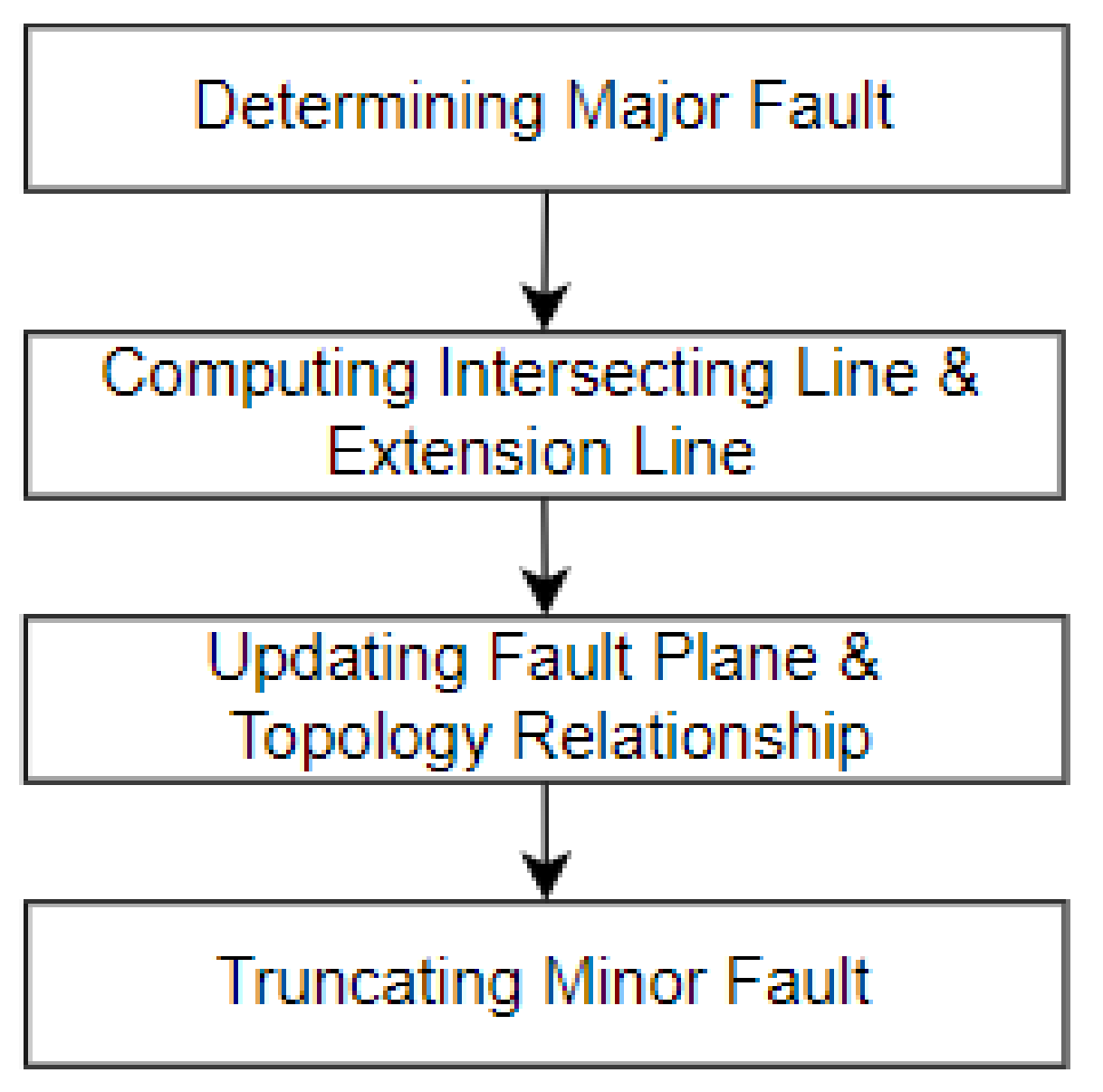
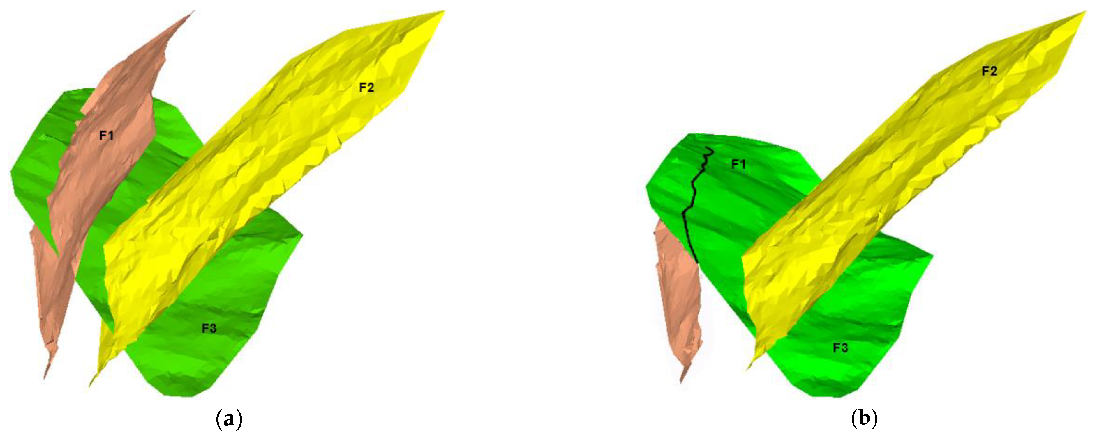
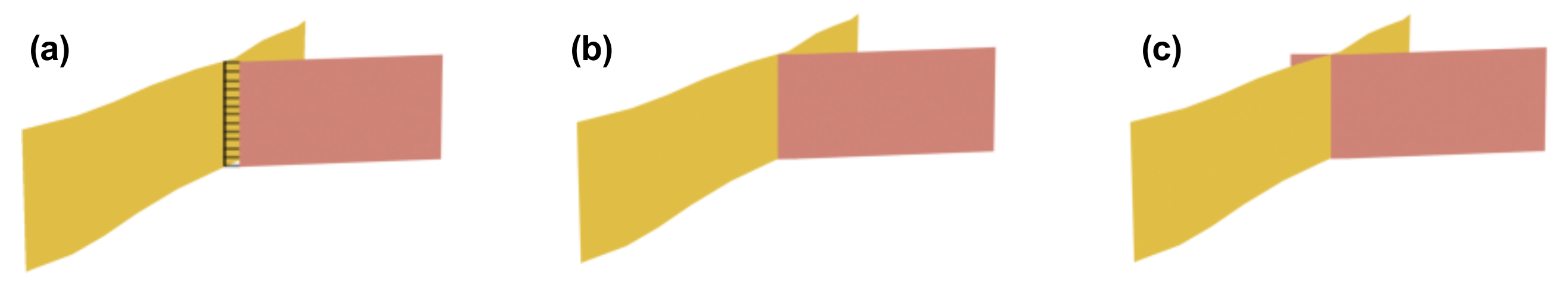
3.2.4. Judging the Truncated Part

When the relationships between the intersecting faults are defined, the minor fault is appropriately truncated. Taking the intersection line and its extension as the boundary, the minor fault can be divided into two parts: the upper and lower parts, and the truncated part is separated from the fault model. Usually, the smaller spread part is truncated. There are some labels: The upper part is truncated as ‘up’; the lower part is truncated as ‘down’; and not truncated as ‘none.’ Obviously, the lower part of $F_2$ in Figure 12a will be truncated and marked as ‘down’ in the relation XML. However, if the truncated part of a certain fault is known from prior geological knowledge, then the known part is truncated directly without judgment. For example, it is known that the upper part of $F_1$ in Figure 12a is truncated by $F_3$, and the upper part after the truncation is separated, marked as ‘up’, with the black track on $F_3$ as truncation line.

3.3. Complex Fault Model Recording Methods

The 3D complex fault model needs to record the fault surface information and the fault-fault contact relationship. The fault surface is regarded as the entity model, and the fault surface contact relationship is the relationship model of the entities. The relationship model records the intersection information of a fault. XML is an effective tool for building entity and relationship models [35], which can accurately describe entity-related relationships. This paper proposes a method of recording complex fault models based on the XML, which can accurately describe the contact relationship between fault surfaces and effectively record complex fault information. The complex fault model recording method records information on fault surfaces, fault-fault contact relationships, and complex fault models in sequence.

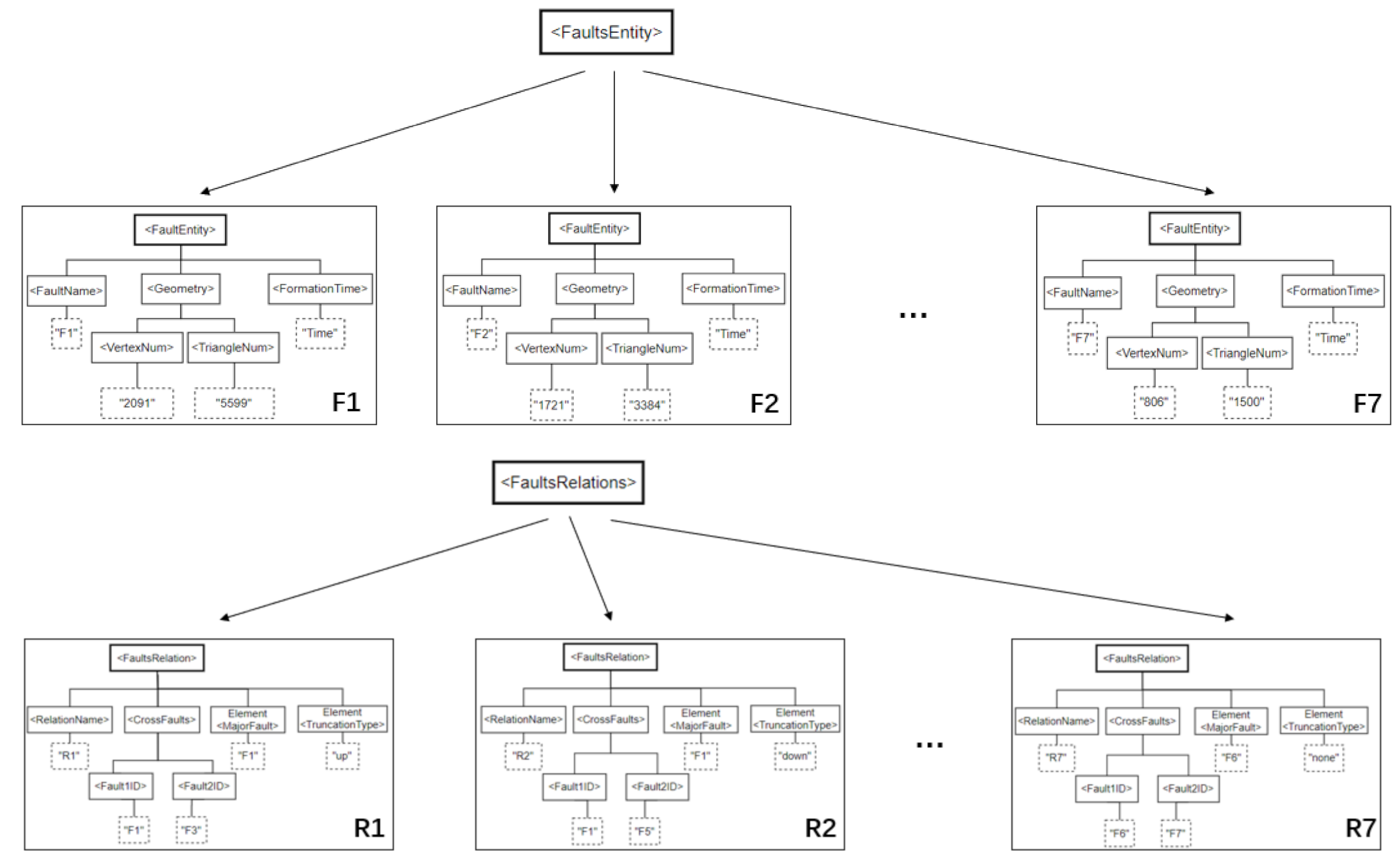
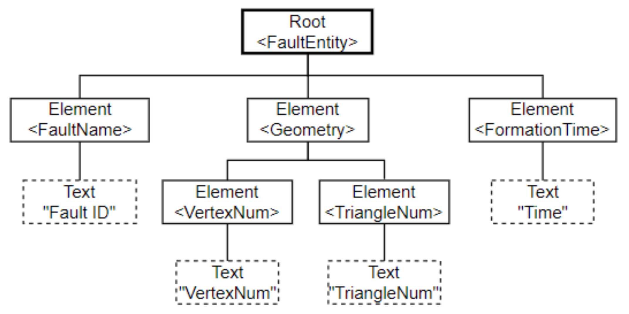
3.3.1. Record the Fault Surfaces

Construct a fault entity model to record the fault information. The set of fault surface entities $E$ contains $n$ entities, $E=\{e_1,e_2,\dots ,e_n\}$, and each entity represents a fault surface.

Table 1. Record Template of Fault Surface Entity Model.

Faults Entity	Information	Details
Faults entity	Fault name	Fault ID
	Geometry	Vertexes
		Triangles
	Formation time	Time

shows the record template of the fault surface entity, which contains three types of elements: the name of the fault represented by the fault ID, the geometric elements of the fault composed of vertices and triangles, and the time of fault formation.

The fault entity model record template is represented by the XML structure diagram shown in Figure 13.

The fault entity model is expressed as an example in xml as follows:

<FaultsEntity>

  <FaultName>F1</FaultName>

  <FaultGeom>

    <Vertex>1721</Vertex>

    <Triangle>3384</Triangle>

  </FaultGeom>

  <FaultTime>Time</FaultTime>

</FaultsEntity>

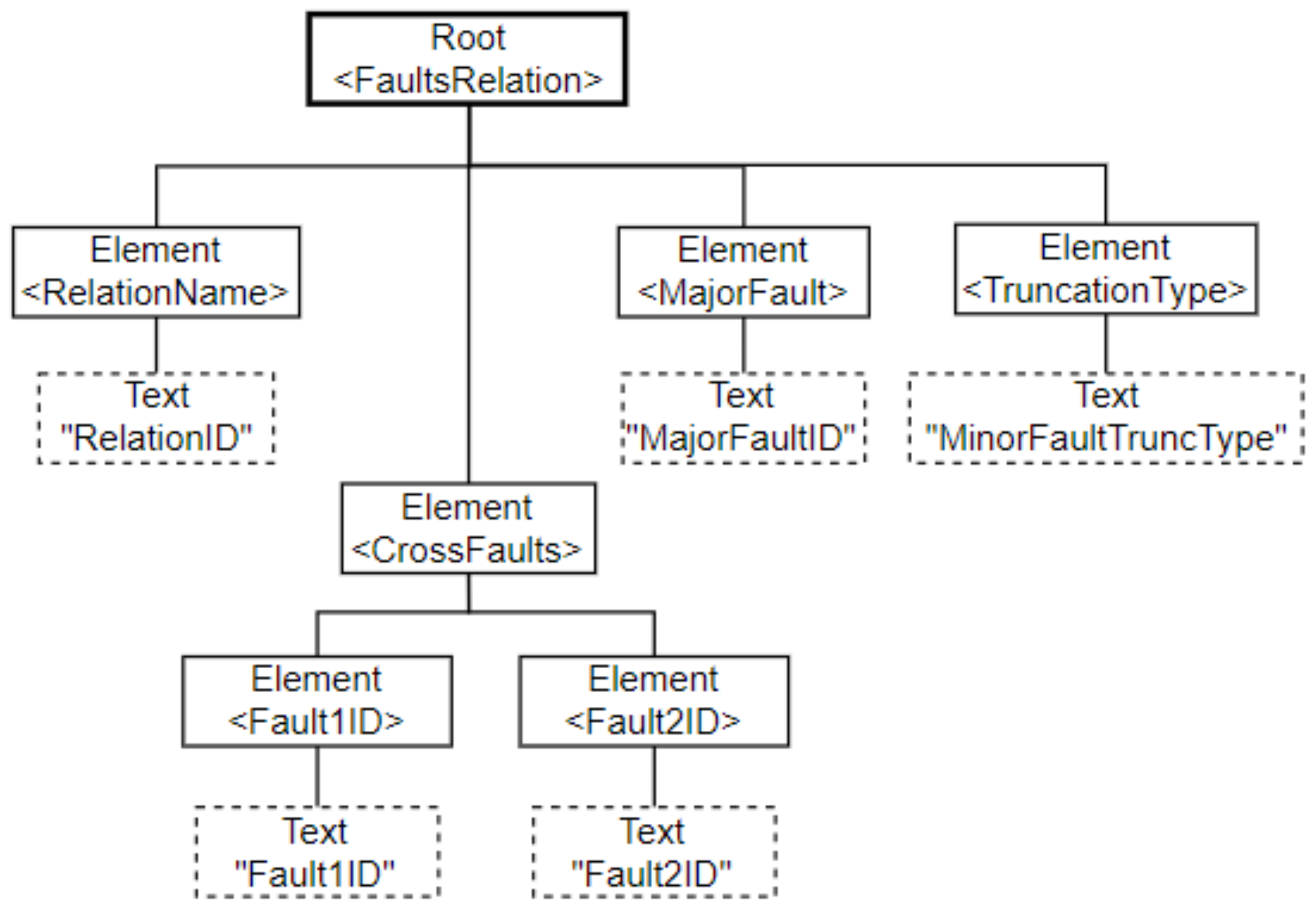
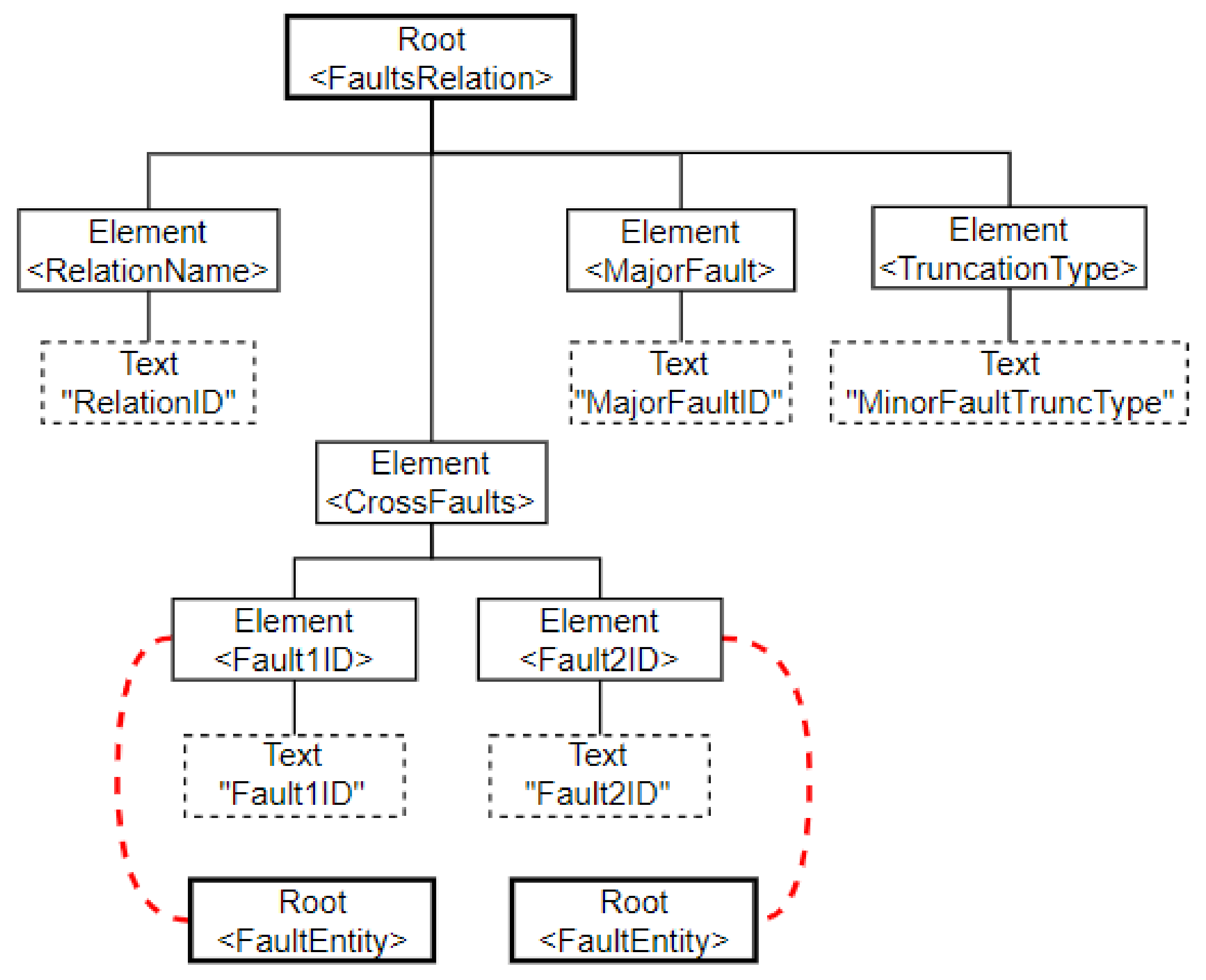
3.3.2. Record the Fault-Fault Contact Relationship

The fault-fault contact relationship was recorded using a relationship model. The set $R$ of fault-fault contact relationships contains $m$ relationships, $R=\{r_1,r_2,\dots ,r_m\}$, each of $r_m=\{e_i,e_j\}$, which represents the intersection of two fault entities $e_i$ and $e_j$. If there is no intersection relationship between the fault entities, no record is required.

Table 2. Record Template of Faults Relationship Model.

Faults Group ID	Information	Details
Faults relation	Relation name	Relation ID
	Cross faults	Fault1 ID
		Fault2 ID
	Major fault	Major fault ID
	Truncation type	Minor fault Truncation type

is a record template of the fault relationship model, including four types of elements: fault relationship name, two intersecting fault IDs, major fault ID, and truncation type of minor faults.

The fault relationship model record template is represented by an XML structure diagram, as shown in Figure 14.

The faults relationship model is expressed as follows in XML:

<FaultsRelations>

  <RelationName>R1</RelationName>

  <CrossFault>

    <Fault1>F1</Fault1>

    <Fault2>F2</Fault2>

  </CrossFault>

  <MajorFault>F1</MajorFault>

  <TruncationType>‘up’</ TruncationType >

</FaultsRelations>

When recording the contact relationship between faults, the judgment of the major and minor faults and the type of truncation are mainly based on the time of formation and the spread size of the geometric spatial distribution of the fault surface. When the model is generated, automatic truncation based on the abovementioned basis is likely to cause missing faults. When recording a complex model, the major and minor fault labels in the fault-fault contact relationship are updated according to the actual contact situation.

3.3.3. Record the Complex Fault Model

The complex fault model is composed of a fault entities model and a contact relationship model between the fault entities. Graph theory is a mathematical model used to describe the relationship between things [38], in which undirected graphs are suitable for describing the structure of complex fault models. Using graphs to represent a complex fault model can ignore the geometric details of the fault model and only pay attention to the topological relationship between faults, making model adjustment more intuitive [33,39].

In the mathematical model, the graph is represented as:

$$G=\{V,E\}$$

This is a two-tuple, in which $V=\{v_1,v_2,\dots ,v_m,v_n\}$ represents the point elements in the graph, and $E=\{v_1{v}_2,v_2{v}_3,\dots ,v_m{v}_n\}$ is a set of edges composed of points that have correlations in $V$ [33].

The fault entities in the complex fault model are equivalent to the point elements in the graph, and the contact relationship between the two faults is equivalent to the edges in the graph (Figure 15). Some of the concepts in graph theory can also correspond to the problems studied in complex fault models. The degree of a point element $D$ indicates the number of edges adjacent to the point, that is, the number of faults that intersect with the fault entity. The disconnected state in the graph theory indicates that there is no intersection relationship between the faults, and the circle indicates the self-truncating phenomenon in the fault, and the isolated point indicates that the fault has no intersection relationship in the model.

In Figure 15, the degree of the point $F_1$ is 3, and the fault entity $F_1$ intersects with three faults, $F_3$, $F_4$, and $F_5$, and the points $F_1$, $F_2$, and $F_3$ form a circle in the graph, indicating that, $F_1$, $F_2$, and $F_3$ are the self-truncating faults that intersect each other in pairs.

The complex fault model associates the fault entities to the relationship model and is represented by the XML structure in Figure 16.

When generating a complex fault model, the labels of the major and minor faults in the fault-fault contact relationship may be changed. The change rules are as follows:

• Remove isolated fault entity points and fault entity points with only two fault entities connected.
• Process the remaining connected fault entities sequentially. The degree of the fault entity $F_i$ is $D_i$ in the fault-fault contact relationship; $r_m=\{e_i=F_i,e_j=F_j\}$ if $D_i>D_j$, then $F_i$ is the major fault and $F_j$ is the minor fault; otherwise, it remains unchanged.
• If a circle is present, a self-truncating fault exists. The judgment of major and minor faults of self-truncating faults is too complicated, so they are not truncated, and its truncation label is marked as ‘none.’

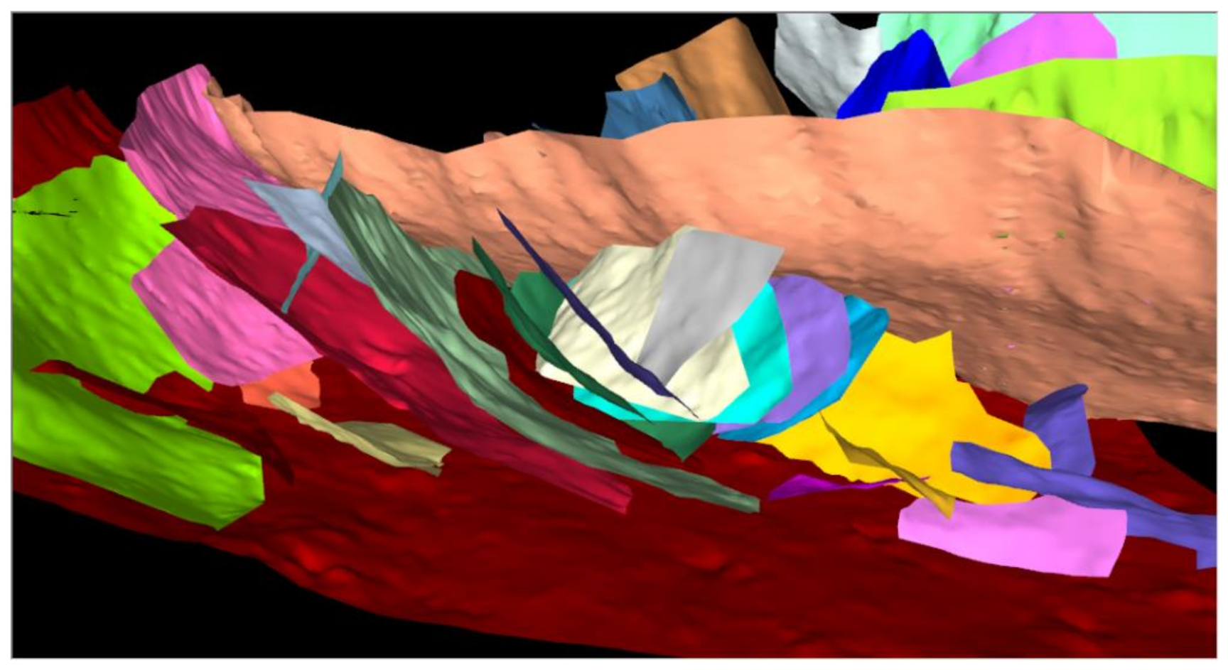
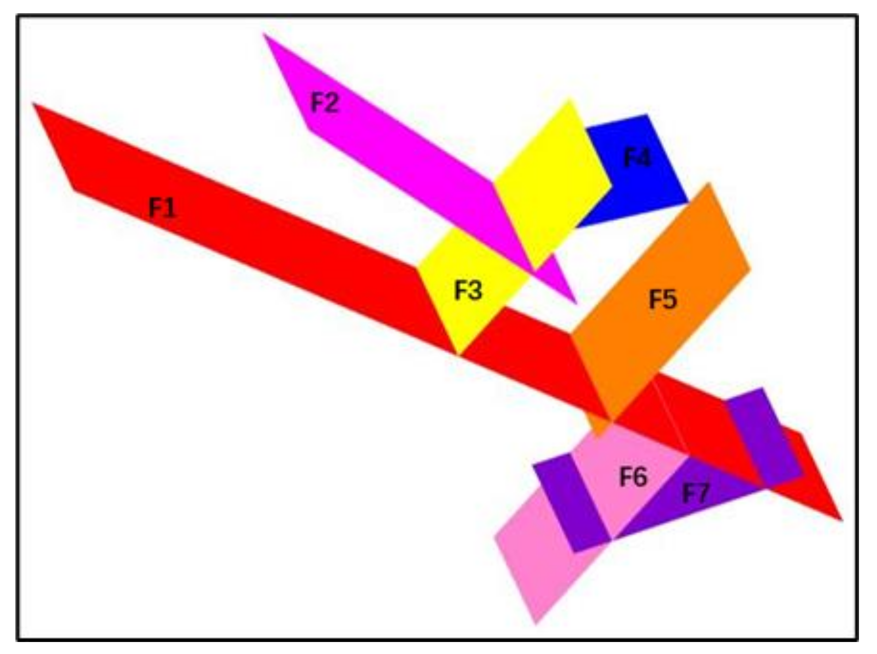
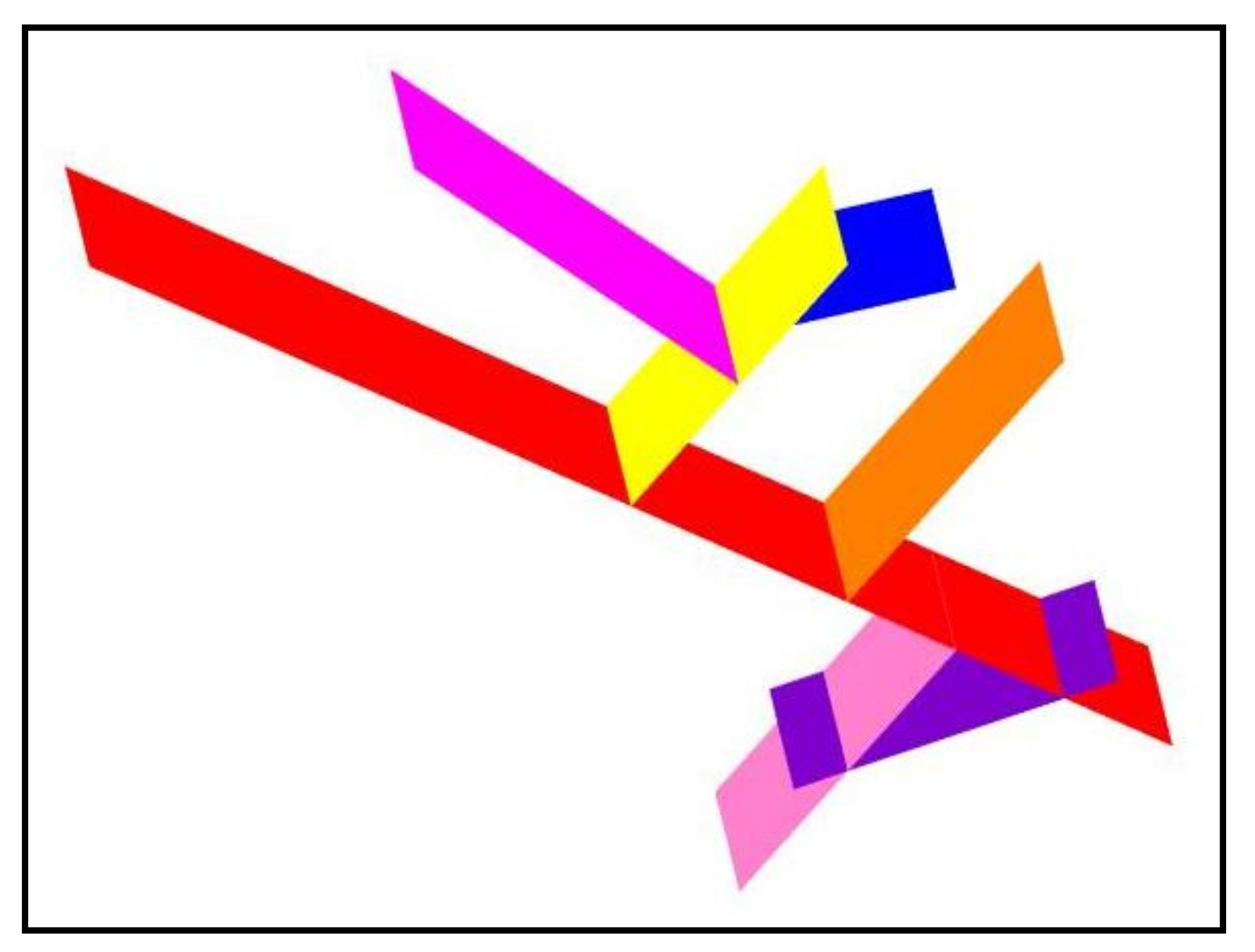
4. Examples of 3D Complex Fault Model Construction

The method proposed in this paper can solve the automatic construction of complex faults including X-type faults, multilevel y-type or λ-type faults, and self-interrupted faults. Figure 17 is a complex fault model composed of seven faults with multilevel and self-truncating characteristics. Each fault is regarded as a fault entity $e_i=F_i$, and the contact relationship between the fault entities is regarded as a relationship entity $r_m$.

The modeling process is as follows:

• Generate fault-fault contact relationship entities.

According to the fault-fault contact relationship in Figure 17, we can obtain $r_1=\{e_1,e_3\}$, $r_2=\{e_1,e_5\}$, $r_3=\{e_1,e_6\}$, $r_4=\{e_1,e_7\}$, $r_5=\{e_2,e_3\}$, $r_6=\{e_3,e_4\}$, $r_7=\{e_6,e_7\}$, $e_i=F_i$, and $R=\{r_1,r_2,r_3,r_4,r_5,r_6,r_7\}$.

2.

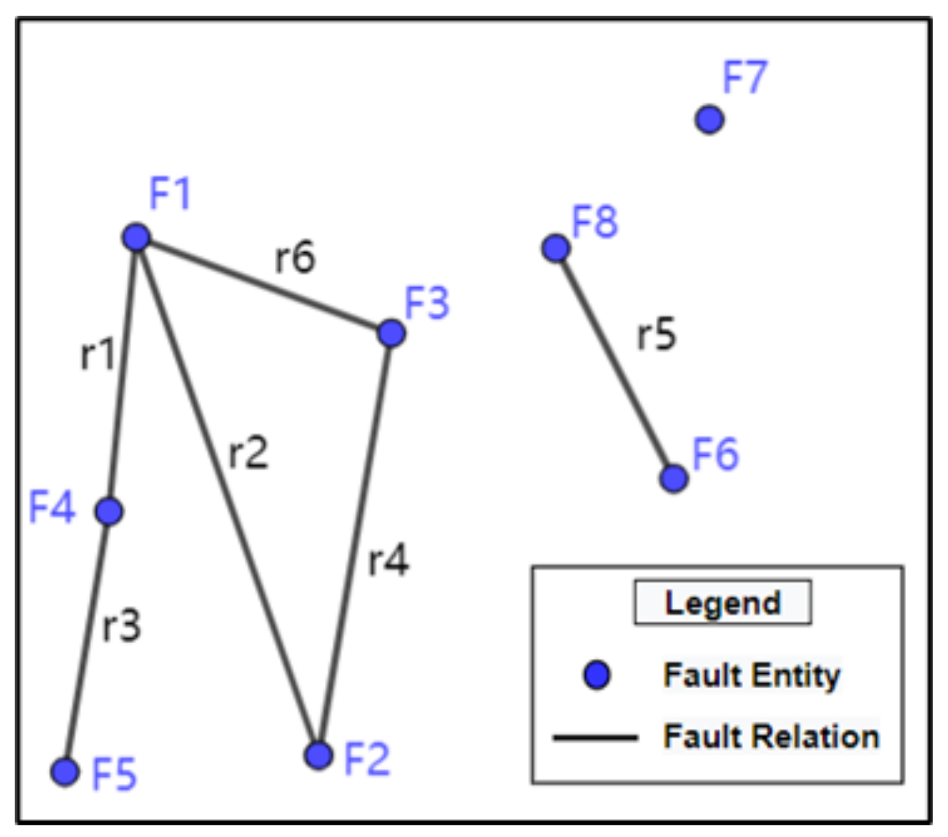
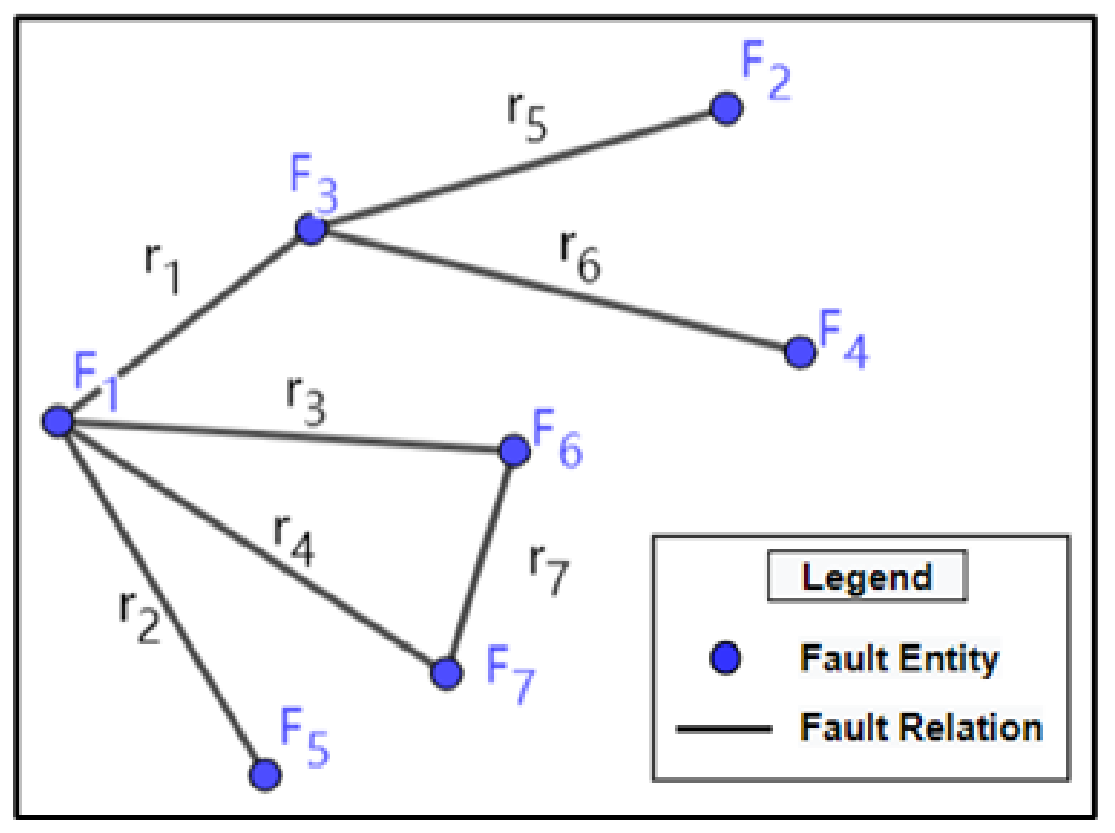
Generate a graph model of a complex fault structure.

The point represents the fault entity, the edge represents the fault-fault contact relationship entity, and the graph model is constructed based on the fault-fault contact relationship entity shown in Figure 18.

3.

Update the label of the major fault and minor fault.

The major fault in the fault relationship entity $r_m$ was recorded as $r_{m}Ma$. In the model in Figure 17, $r_{1}Ma=e_1$, $r_{2}Ma=e_1$, $r_{3}Ma=e_1$, $r_{4}Ma=e_1$, $r_{5}Ma=e_2$, $r_{6}Ma=e_4$, and $r_{7}Ma=e_6$. Update the major fault label according to Figure 18. Calculate the degree $D$ of each node in Figure 18 and determine the existence of the circle $C=\{F_1{F}_6,F_6{F}_7,F_7{F}_1\}$ in the graph shown in Figure 18.

$$D=\{D_1=4,D_2=1,D_3=3,D_4=1,D_5=1,D_6=2,D_7=2\}$$

After the update, the major fault in $r_5$ changed from $e_2$ to $e_3$ (

Table 3. Results of updating the major fault labels.

Fault Entity	New Major Fault
$r_1$	$r_{1}Ma=e_1$
$r_2$	$r_{2}Ma=e_1$
$r_3$	$r_{3}Ma=e_1$
$r_4$	$r_{4}Ma=e_1$
$r_5$	$r_{5}Ma=e_3$
$r_6$	$r_{6}Ma=e_4$
$r_7$	$r_{7}Ma=e_6$

), and the truncation label in $r_3,r_4,r_7$ changed to ‘none.’

The schematic diagram of XML record examples of the model is shown in Figure 19 and the XML codes are listed in the Appendix A. The result of the complex fault model is shown in Figure 20.

5. Discussion and Conclusions

Based on the labeled fault point data, this study proposes and realizes the key process of automatic construction of complex fault network model, using 3D TIN fault surface model. This method has achieved good application effects in one area of China (Figure 21), replacing at least 1–2 days of manual interaction with a few minutes of computer automation. This method has the following advantages:

• It can automatically establish complex fault type such as x-shaped faults, multilevel y-shaped or λ-shaped faults, and self-truncating faults.
• It can automatically determine the fault-fault contact relationship of complex faults and independently truncate the minor faults, which greatly reduces the degree of manual participation in the model building process.
• XML was used to record complex fault models’ information. It can be converted with a graph structure to facilitate the analysis of the contact relationship between faults in a visual environment. Prior geological knowledge can be expressed in XML and directly participate in model construction, simplifying modeling steps and improving modeling efficiency.

Going forward, the standard for automatic judgment of fault type and truncation part for particularly complex fault models will still need to be further explored.

References

1. Caumon, G.; Collon-Drouaillet, P.; de Veslud, C.L.; Viseur, S.; Sausse, J. Surface-Based 3D Modeling of Geological Structures. Math. Geosci. 2009, 41, 927–945. [Google Scholar] [CrossRef] [Green Version]
2. Jessell, M.; Ailleres, L.; De Kemp, E.; Lindsay, M.; Wellmann, F.; Hillier, M.; Martin, R. Next Generation Three-Dimensional Geologic Modeling and Inversion. Soc. Econ. Geol. Spec. Publ. 2014, 18, 261–272. [Google Scholar]
3. Wellmann, F.; Caumon, G. 3-D Structural geological models: Concepts, methods, and uncertainties. Adv. Geophys. 2018, 59, 1–121. [Google Scholar]
4. Jessell, M.W. “Noddy”—An interactive Map Creation Package. Master’s Thesis, Imperial College of Science and Technology, London, UK, 1981. [Google Scholar]
5. Jessell, M.W.; Valenta, R.K. Structural geophysics: Integrated structural and geophysical modelling. Comput. Methods Geosci. 1996, 15, 303–324. [Google Scholar]
6. Godefroy, G.; Caumon, G.; Ford, M.; Laurent, G.; Jackson, C.A.L. A parametric fault displacement model to introduce kinematic control into modeling faults from sparse data. Interpret. J. Subsurf. Charact. 2018, 6, B1–B13. [Google Scholar] [CrossRef]
7. Grose, L.; Ailleres, L.; Laurent, G.; Caumon, G.; Jessell, M.; Armit, R. Realistic modelling of faults in LoopStructural 1.0. Geosci. Model Dev. Discuss. 2021, 1–26. [Google Scholar] [CrossRef]
8. Wang, Z.G.; Qu, H.G.; Wu, Z.X.; Wang, X.H. Geo3DML: A standard-based exchange format for 3D geological models. Comput. Geosci. 2018, 110, 54–64. [Google Scholar] [CrossRef]
9. Wang, Z.G.; Qu, H.G.; Wu, Z.X.; Yang, H.J.; Du, Q.L. Formal representation of 3D structural geological models. Comput. Geosci. 2016, 90, 10–23. [Google Scholar] [CrossRef]
10. Jessell, M.; Ogarko, V.; Lindsay, M.; Joshi, R.; Pirot, G. Automated geological map deconstruction for 3D model construction. Geosci. Model Dev. Discuss. 2021, 1–35. [Google Scholar] [CrossRef]
11. Wu, X.; Hale, D. 3D seismic image processing for faults. Geophysics 2016, 81, IM1–IM11. [Google Scholar] [CrossRef] [Green Version]
12. Wu, X.; Shi, Y.; Fomel, S. Using Synthetic Data Sets to Train a Neural Network for Three-Dimensional Seismic Fault Segmentation. U.S. Patent No. US20210158104A1, 27 May 2021. [Google Scholar]
13. Qi, J.; Machado, G.; Marfurt, K. A workflow to skeletonize faults and stratigraphic features. Geophysics 2017, 82, O57–O70. [Google Scholar] [CrossRef]
14. Wei, K. 3D Fast Fault Restoration. U.S. Patent No. US 7,480,205 B2, 20 January 2009. [Google Scholar]
15. Lepage, F.L.; Souche, A. Faulted Geological Structures Containing Unconformities. U.S. Patent No. 9,378,312, 12 September 2013. [Google Scholar]
16. Thom, J.; Hocker, C. 3-D Grid Types in Geomodeling and Simulation–How the Choice of the Model Container Determines Modeling Results Grid Types in Geological Modeling. In Proceedings of the AAPG Annual Convention and Exhibition, Denver, CO, USA, 7–10 June 2009. [Google Scholar]
17. Al-shamali, A.; Al-Mayyas, E.A.; Murthy, N.; Verma, N.K.; Al-Sammak, I.; Zhou, C.; Perumalla, S.V.; Shinde, A.L. Geomechanical Characterization of a Matured Deep Jurassic Carbonate Reservoir: Explaining stress effects on production induced Fault Slip and Reservoir Development. In Proceedings of the SPE Reservoir Characterisation and Simulation Conference and Exhibition, Abu Dhabi, United Arab Emirates, 14–16 September 2015. [Google Scholar] [CrossRef]
18. Qu, D.; Roe, P.; Tveranger, J. A method for generating volumetric fault zone grids for pillar gridded reservoir models. Comput. Geosci. 2015, 81, 28–37. [Google Scholar] [CrossRef] [Green Version]
19. Wang, P.Y.; Li, Y.H.; Li, Z.Y. Methods of Fault Modeling by Well-to-Seismic Integration. Appl. Mech. Mater. 2015, 733, 178–181. [Google Scholar] [CrossRef]
20. Prothro, L.B.; Wagoner, J. Geologic Framework Model for the Dry Alluvium Geology (DAG) Experiment Testbed, Yucca Flat; Nevada National Security Site (NNSS): North Las Vegas, NV, USA, 2020. [Google Scholar] [CrossRef]
21. Abbott, W.E. Method and Apparatus for Determining Geologic Relationships for Intersecting Faults. U.S. Patent No. 5,982,707, 9 November 1999. [Google Scholar]
22. Caumon, G.; Lepage, F.; Sword, C.H.; Mallet, J.L. Building and editing a sealed geological model. Math. Geol. 2004, 36, 405–424. [Google Scholar] [CrossRef]
23. Tertois, A.L.; Mallet, J.L. Editing faults within tetrahedral volume models in real time. Geol. Soc. Lond. Spec. Publ. 2007, 292, 89–101. [Google Scholar] [CrossRef]
24. Graf, K.E.; Vassilev, A.T. Automatic Non-Artificially Extended Fault Surface Based Horizon Modeling System, Part I. U.S. Patent No 6,014,343, 11 January 2000. [Google Scholar]
25. Hoffman, K.S.; Neave, J.W.; Nilsen, E.H. Building Complex Structural Frameworks. In Proceedings of the International Oil Conference and Exhibition in Mexico, Veracruz, Mexico, 27–30 June 2007. [Google Scholar] [CrossRef]
26. Hoffman, K.S.; Neave, J.W. The fused fault block approach to fault network modelling. Geol. Soc. Lond. Spec. Publ. 2007, 292, 75–87. [Google Scholar] [CrossRef]
27. Neave, J.W. Analysis and Characterization of Fault Networks. U.S. Patent No. US 7,512,529 B2, 31 March 2009. [Google Scholar]
28. Nyberg, B.; Nixon, C.W.; Sanderson, D.J. NetworkGT: A GIS tool for geometric and topological analysis of two-dimensional fracture networks. Geosphere 2018, 14, 1618–1634. [Google Scholar] [CrossRef] [Green Version]
29. Sanderson, D.J.; Peacock, D.C.P.; Nixon, C.W.; Rotevatn, A. Graph theory and the analysis of fracture networks. J. Struct. Geol. 2019, 125, 155–165. [Google Scholar] [CrossRef] [Green Version]
30. Morley, C.K.; Binazirnejad, H. Investigating polygonal fault topological variability: Structural causes vs image resolution. J. Struct. Geol. 2020, 130, 103930. [Google Scholar] [CrossRef]
31. Thiele, S.T.; Jessell, M.W.; Lindsay, M.; Ogarko, V.; Wellmann, F.; Pakyuz-Charrier, E. The topology of geology 1: Topological analysis. J. Struct. Geol. 2016, 91, 27–38. [Google Scholar] [CrossRef]
32. Thiele, S.T.; Jessell, M.W.; Lindsay, M.; Wellmann, F.; Pakyuz-Charrier, E. The topology of geology 2: Topological uncertainty. J. Struct. Geol. 2016, 91, 74–87. [Google Scholar] [CrossRef]
33. Godefroy, G.; Caumon, G.; Laurent, G.; Bonneau, F. Structural Interpretation of Sparse Fault Data Using Graph Theory and Geological Rules. Math. Geol. 2019, 51, 1091–1107. [Google Scholar] [CrossRef] [Green Version]
34. Li, Z.; Pan, M.; Yang, Y.; Cao, K.; Wu, G. Research and Application of the Three-Dimensional Complex Fault Network Modeling. Acta Sci. Nat. Univ. Pekin. 2015, 51, 79–85. [Google Scholar]
35. W3C. Extensible Markup Language (XML); W3C Standards. 2015. Available online: www.w3.org/standards/xml/core (accessed on 17 August 2021).
36. Lee, D.T.; Schachter, B.J. Two algorithms for constructing a Delaunay triangulation. Int. J. Parallel Program. 1980, 9, 219–242. [Google Scholar] [CrossRef]
37. Mei, G.; Tipper, J.C.; Xu, N. Ear-Clipping Based Algorithms of Generating High-Quality Polygon Triangulation. In Proceedings of the 2012 International Conference on Information Technology and Software Engineering. Lecture Notes in Electrical Engineering; Lu, W., Cai, G., Liu, W., Xing, W., Eds.; Springer: Berlin/Heidelberg, Germany, 2013; Volume 212. [Google Scholar] [CrossRef] [Green Version]
38. Barnett, J.H. Early Writings on Graph Theory: Euler Circuits and The Königsberg Bridge Problem An Historical Project; Colorado State University: Pueblo, CO, USA, 2005; Available online: https://www-users.cse.umn.edu/~reiner/Classes/Konigsberg.pdf (accessed on 17 August 2021).
39. Thomson, B. Topology vs. Topography: Sometimes Less is More. In Proceedings of the Second EAGE Integrated Reservoir Modelling Conference, Dubai, United Arab Emirates, 16–19 November 2014. [Google Scholar]
Figure 1. Flow chart of complex fault model construction.
Minerals 11 00893 g001
Figure 2. Schematic diagram of 2D projection and the reference planar. The 3D fault points A, B, C, D, and N are projected to the 2D reference planar S, corresponding to points A1, B1, C1, D1, and N1.
Minerals 11 00893 g002
Figure 3. Schematic diagram of type about fault-fault contact relationship [34]. (a): disjoint fault surfaces; (b): intersection stopping fault surfaces; (c): intersection cutting fault surfaces. Reprinted with permission from ref. [34], copyright 2015 Acta Scientiarum Naturalium Universitatis Pekinensis publisher.
Minerals 11 00893 g003
Figure 4. Automatic generation process of 3D fault surface.
Minerals 11 00893 g004
Figure 5. Automatic calculation process of fault contact relationship.
Minerals 11 00893 g005
Figure 6. Schematic diagram of the intersection of triangles (The triangular patch TA in the fault surface T intersects with the triangular patches SA, SB, and SC of the fault surface S at the same time, resulting in four intersection points and the intersecting polyline).
Minerals 11 00893 g006
Figure 7. Schematic diagram of truncation rules. The (a) has an intersection line that directly cuts across the two faults surface, and the fault surface of (bd) are all partially cut across. Usually, the smaller spread part is truncated. The truncated results are showed in (eh). The red fault partially extends over the blue fault surface in (bd), which may exist in practice, so we maintain these parts as they used to be.
Minerals 11 00893 g007
Figure 8. Schematic diagram of the extension of the intersection line of the fault surface.
Minerals 11 00893 g008
Figure 9. Schematic diagram of three kinds of triangle closed polygon. (a) has two points at the edge. (b) has one point at the edge. (c) has all points inside the triangle.
Minerals 11 00893 g009
Figure 10. Schematic diagram of triangulation cutting of intersecting triangles. Deleting all points on the closed polygon except the vertex in (a) to generate (b).
Minerals 11 00893 g010
Figure 11. Example of triangulation of intersecting surface. (a) shows two intersecting planes. (b) shows two intersecting surfaces with geometrical topology consistency.
Minerals 11 00893 g011
Figure 12. Example diagram of truncation of intersecting fault surfaces. (b) is the truncating result of (a).
Minerals 11 00893 g012
Figure 13. Diagram of XML structure of fault entity.
Minerals 11 00893 g013
Figure 14. Diagram of XML structure of faults relationship model.
Minerals 11 00893 g014
Figure 15. Schematic diagram of structure diagram of complex fault model.
Minerals 11 00893 g015
Figure 16. Schematic diagram of XML description template of complex fault model.
Minerals 11 00893 g016
Figure 17. Example of a complex fault model.
Minerals 11 00893 g017
Figure 18. Graph model of complex fault model.
Minerals 11 00893 g018
Figure 19. Schematic diagram of XML record result.
Minerals 11 00893 g019
Figure 20. Schematic diagram of the results of complex fault model construction.
Minerals 11 00893 g020
Figure 21. Schematic diagram of the results of complex fault model construction.
Minerals 11 00893 g021