Review

Trace Metal Contamination of Bottom Sediments: A Review of Assessment Measures and Geochemical Background Determination Methods

1
Faculty of Civil and Environmental Engineering, Gdańsk University of Technology, 80-233 Gdansk, Poland
2
School of Forest Sciences, University of Eastern Finland, Yliopistokatu 7, P.O. Box 111, 80100 Joensuu, Finland
3
Department of Environment and Energy, Sejong University, Seoul 05006, Korea
*
Author to whom correspondence should be addressed.
Minerals 2021, 11(8), 872; https://doi.org/10.3390/min11080872
Submission received: 16 June 2021 / Revised: 9 August 2021 / Accepted: 10 August 2021 / Published: 12 August 2021
(This article belongs to the Special Issue Elemental Concentration and Pollution in Soil, Water, and Sediment)

Abstract

:
This paper provides an overview of different methods of assessing the trace metal (TM) contamination status of sediments affected by anthropogenic interference. The geochemical background determination methods are also described. A total of 25 papers covering rivers, lakes, and retention tanks sediments in areas subjected to anthropogenic pressure from the last three years (2019, 2020, and 2021) were analysed to support our examination of the assessment measures. Geochemical and ecotoxicological classifications are presented that may prove useful for sediment evaluation. Among the geochemical indices, several individual pollution indices (CF, Igeo, EF, Pi (SPI), PTT), complex pollution indices (PLI, Cdeg, mCdeg, Pisum, PIAvg, PIaAvg, PIN, PIProd, PIapProd, PIvectorM, PINemerow, IntPI, MPI), and geochemical classifications are compared. The ecotoxicological assessment includes an overview of Sediment Quality Guidelines (SQG) and classifications introduced nationally (as LAWA or modified LAWA). The ecotoxicological indices presented in this review cover individual (ERi) and complex indices (CSI, SPI, RAC, PERI, MERMQ). Biomonitoring of contaminated sites based on plant bioindicators is extensively explored as an indirect method for evaluating pollution sites. The most commonly used indices in the reviewed papers were Igeo, EF, and CF. Many authors referred to ecotoxicological assessment via SQG. Moreover, PERI, which includes the toxic response index, was just as popular. The most recognised bioindicators include the Phragmites and Salix species. Phragmites can be considered for Fe, Cu, Cd, and Ni bioindication in sites, while Salix hybrid cultivars such as Klara may be considered for phytostabilisation and rhizofiltration due to higher Cu, Zn, and Ni accumulation in roots. Vetiveria zizanoides demonstrated resistance to As stress and feasibility for the remediation of As. Moreover, bioindicators offer a feasible tool for recovering valuable elements for the development of a circular economy (e.g., rare earth elements).

1. Introduction

Nowadays, the contamination of sediments with trace metals (TMs) is a salient environmental issue [1,2]. TMs delivered to the environment from anthropogenic sources are mostly represented by these elements: Cd, Co, Cr, Cu, Fe, Hg, Mn, Mo, Ni, Pb, Sn, V, and Zn. Supplementation from external sources also includes other potentially toxic elements (PTEs) such as metalloids (As, Sb) and non-metals (Se) [3]. PTEs are not biodegradable, persistent, and can accumulate in the environment in large amounts. TM ions cause health hazards; just to mention a few, these include emphysema (Cd), anaemia (Cd, Zn, Pb), damage to the brain (Pb), kidneys, and bones (Cd), necrosis nephritis (Cr), DNA damage (Ni), eczema on the hands (Ni), risk of developing cancer (As), central nervous system irritation (Cu), and even death in humans [4]. Due to the toxic nature of PTEs, there is an obvious need to monitor their content. The most significant anthropogenic sources of PTEs are related to industry, urbanisation, transportation, agriculture, and mines [5,6,7,8] TMs adhered to particulate matter (PM; including PM10 and PM2.5) could be released into the surrounding environment causing contamination of soils, groundwaters, sediments, and surface waters. PTEs entering the aquatic ecosystem are associated with fine-grained fractions of suspended solids and sediments due to their large surface areas and high sorption capacities [9]. Throughout the hydrological cycle, 99% of PTEs are stored in sediments, which, therefore, act as the main sinks and carriers for contaminants in aquatic environments [10]. Contemporary studies [11,12,13,14,15,16,17,18] have revealed that stormwater run-off carried metals originating from various sources of everyday use associated with tyre wear, corrosion, roof run-off, and fuel combustion products. Zn, Pb, Cu, Cd, Ni, Ce, and As are typically observed in urban and industrial catchments [11,12].
Sediments are the ultimate repository for contaminants and provide valuable information about the environmental status of a catchment area [17]. According to USEPA [19], sediment site management and silting processes in reservoirs present a unique challenge because of the large number of difficult to control contaminant sources, dynamic phenomena influencing movement and sediment stability, dispersion of contaminants, diversified use of areas affecting the sediment environment, as well as difficulties involved in engineering cleanup works.
Sediment contamination may be evaluated in several ways. Geochemical, ecotoxicological, and bioindicator-related approaches can be distinguished. Extensive evaluation includes geochemical and ecotoxicological methods. The geochemical assessment relies on comparing TMs at particular sites to the geochemical background or baseline. The term “geochemical background” (or “natural background”) has evolved. In exploration geochemistry, it refers to the non-anomalous concentration of elements in the rocks surrounding the mineral ore body. In environmental sciences, it is used to detect anthropogenic impact on the environment [20]. Establishing the geochemical background raises research concerns because it may determine the overall pollution status of an examined site. Ecotoxicological approaches are based on assessing the effects of metal toxicity on living organisms and determining certain dose limits. Bioindication is an indirect method of verifying the quality of the environment—i.e., by using aquatic plants and hydrophytes able to accumulate a large number of metals, making them suitable for environmental biomonitoring. The distribution and behaviour of aquatic plants are frequently correlated with water and sediment quality [21]. Macrophytes are able to accumulate pollutants at a higher level, irrespective of their content in the surrounding environment [22]. Moreover, the analyses of plant tissues provide time-integrated information about the quality of an examined site, even if contaminant inputs are discontinuous and quickly diluted in water [23]. One of the species widely recognised as featuring correlations between concentration of metals in sediment/soil and roots is Phragmites australis [15]. Hydrophytes uptake PTEs through their roots and rhizomes, stems, and leaves [24]. Plant species with a strong ability to accumulate TMs in the aboveground tissues are good candidates for phytoextraction [25].
The most simple way to evaluate TM contamination of sediments is based on total metal content. This approach reflects the geological origin and anthropogenic influence, although it is ineffective in terms of documenting mobility or bioavailability [26]. According to Ure and Davidson [27], a more accurate method taking into account these two features is to measure the “pseudo total” metal content in sediments. Pseudo total content presents the maximum potential soluble or mobile metal content, which can be identified with maximum potential hazard. Sequential extraction (or fractionation) distinguishes several factions—mobile, conditionally mobile, and immobile (depending on the applied method). Therefore, using this approach, potential metal contamination hazards can be more accurately assessed and explored. Combining fractionation with different contamination assessment approaches (geochemical and ecotoxicological) may also offer valuable insight into sediment quality.
Sediment contamination is a well-known problem across the world; however, monitoring programs based on different PTE contamination assessment methods as well as bioindicators have to be implemented to ensure that the assessment is credible and reliable. Various studies use different approaches to evaluate the quality of sediments, which impairs the comparison of results from diverse studies. Even the definition of background values, which is a fundamental step in geochemical assessment, is often controversial. Therefore, there are four aims of this review: (1) to summarise the levels of TM content and methods used to evaluate the contamination status of bottom sediments related to surface run-off receivers from the last 3 years, (2) to assemble and critically evaluate the geochemical and ecotoxicological classifications and contamination indices used to evaluate the PTE-polluted sediment and the subsequent risk, (3) to explain the difference between geochemical background and baseline; and (4) to specify the bioindicators of TMs that have been extensively researched at different sites across the world.

2. Materials and Methods

A literature review was conducted via the Web of Science platform. In order to access a complete spectrum of data on PTEs in the bottom sediments of urban water bodies, 5 specific keywords were chosen: sediments, trace metals, contamination, pollution indices, and urban. The Web of Science Core Collection displayed a total of 519 papers, which are available in the database (starting from the year 1994). From the last 3 years (2019, 2020, 2021), there are 202 publications in total, and a further 145 results in the field of environmental science (as of May 2021). We used 25 of the latest publications from the last 3 years (2019, 2020, and 2021). To explore the last 10 years of updates regarding bioindication species, the search process was based on the following keywords: plant bioindicators, metal indicator, Salix or Willow as bioindicator, phytoextraction, and bioindicator.

3. PTEs in Bottom Sediments of Urban Water Bodies

Based on 25 of the latest publications [28,29,30,31,32,33,34,35,36,37,38,39,40,41,42,43,44,45,46,47,48,49,50,51,52] on the topic of bottom sediments in urban waterbodies, Table A1 in Appendix A presents (1) a list of TMs evaluated under each study, (2) their concentration ranges (in mg/kg d.w.), (3) a basic description of the site and land use, (4) indices, classifications, and an evaluation of TM bioavailability with the use of metal fractionation.
In most of the examined papers, the authors focused on five TMs: Cu, Zn, Pb, Ni, Cr, and a metalloid: As. All of the mentioned elements can be delivered by anthropogenic activities such as metalliferous mining, smelters, metallurgy, rolling, electronic, industry, the dye and paint industry, metal corrosion of materials, plastic industry, chemical industry, combustion of fossil fuels, wood industry, as well as tyre wear and lubricant oils [6]. The scope of analyses in many studies also included Fe, Mn, Co, Hg, as well as rare earth elements, i.e., La and Sc.
Most authors sampled the surface layer of sediments (0–2 cm, 0–5 cm, or 0–10 cm), where reactions occur at the water–sediment interface and where living organisms dwell. The sampling strategy is crucial for the successful collection of sediment samples with undisturbed stratification. With this aim, a grab sampler (for surface sediment extraction), hand (core extraction < 60 cm) and box corer (core extraction < 1 m) devices, or a multiple corer can be used to obtain proper samples. Sediment samples are collected to describe the condition of the sites. The specific reasons for sediment sampling include bioassays (the top 10 cm are usually collected because of biological activities), biosurvey (macroinvertebrate analyses), monitoring, examining non-point pollution, and pollutant sources. Monitoring trends and relationships in sediments requires information on current PTE burden in the uppermost sediment layer (e.g., 0–1 cm). Depending on the receiver (large/small body of water, river, stream, bay), the rate of deposition varies, which means that 1 cm of sediment builds up over different times. Therefore, the EU [53] has recommended sampling the top layer of sediment at a depth of 1–5 cm; however, this depends on the deposition rate. This is also in line with data from the United States, which stated that more than 10% of the volume of bottom sediments (the upper 5 cm of surface sediments) are estimated to have been contaminated. The depth to which sediments are sampled should be one of the key monitoring objectives. Core sample collection is crucial for evaluating the PTE footprint. Sediments from depths greater than 15 cm below the sediment–water interface are usually collected to determine the spatial vertical properties and sedimentation history. Each sampling program requires a compromise between the number of samples, sampling frequency, measurement parameters, and cost effectiveness [54].
The most frequently used indices were Geoaccumulation Index (Igeo) (17 studies), Enrichment Factor (EF) (13 studies), Contamination Factor (CF) (10 studies), Pollution Load Index (PLI) (6 studies), Metallic Pollution Index (MPI) and Modified Contamination Degree (mCd) (each used in 3 studies), Nemerow Pollution Index (PINemerow) (2 studies), MRI and Pollution Index (PI) (each used in 1 study). Two studies undertook a sediment assessment using the German classification LAWA, while one study refers to Romanian legislation. Reference to the ecotoxicological assessment via Sediment Quality Guidelines (SQG) was carried out in eight studies, while Ecological Risk Index (Eri), Risk Index (RI), and Potential Ecological Risk Index (PERI) (which account for metal toxicity) were used in 17 studies. Moreover, only two studies assessed health risk. Three papers considered the use of chemical sequential extraction for element analyses, which is important to assess the bioavailability and mobility of TMs. Only one study included a Risk Assessment Code (RAC) analysis, which takes into account the risk determination based on the metal binding to the exchangeable and carbonate fraction. Health risk—as Hazard Index (HI) and Hazard Quotient (HQ)—was calculated in two papers. The common use of indices enables the results to be compared between various studies. However, calculations of geochemical indices are strongly dependent on the adopted reference value (geochemical background).
Another important issue, addressed in three studies, is the fractionation analysis of TMs. Fractionation allows the environmental behaviour of trace elements to be assessed [55]. However, the procedure itself is highly labor-intensive and cost-prohibitive. Most works are based on assessing the total metal content of the samples; nevertheless, fractionation is an indispensable method when it comes to exploring the actual metal bioavailability and mobility.
The above characteristic offers an overview of the most often used indices for geochemical and ecotoxicological evaluation of sediments. The next part of this review presents a “conventional” division of tools for assessment of sediment quality, taking into account geochemical and ecotoxicological approaches.

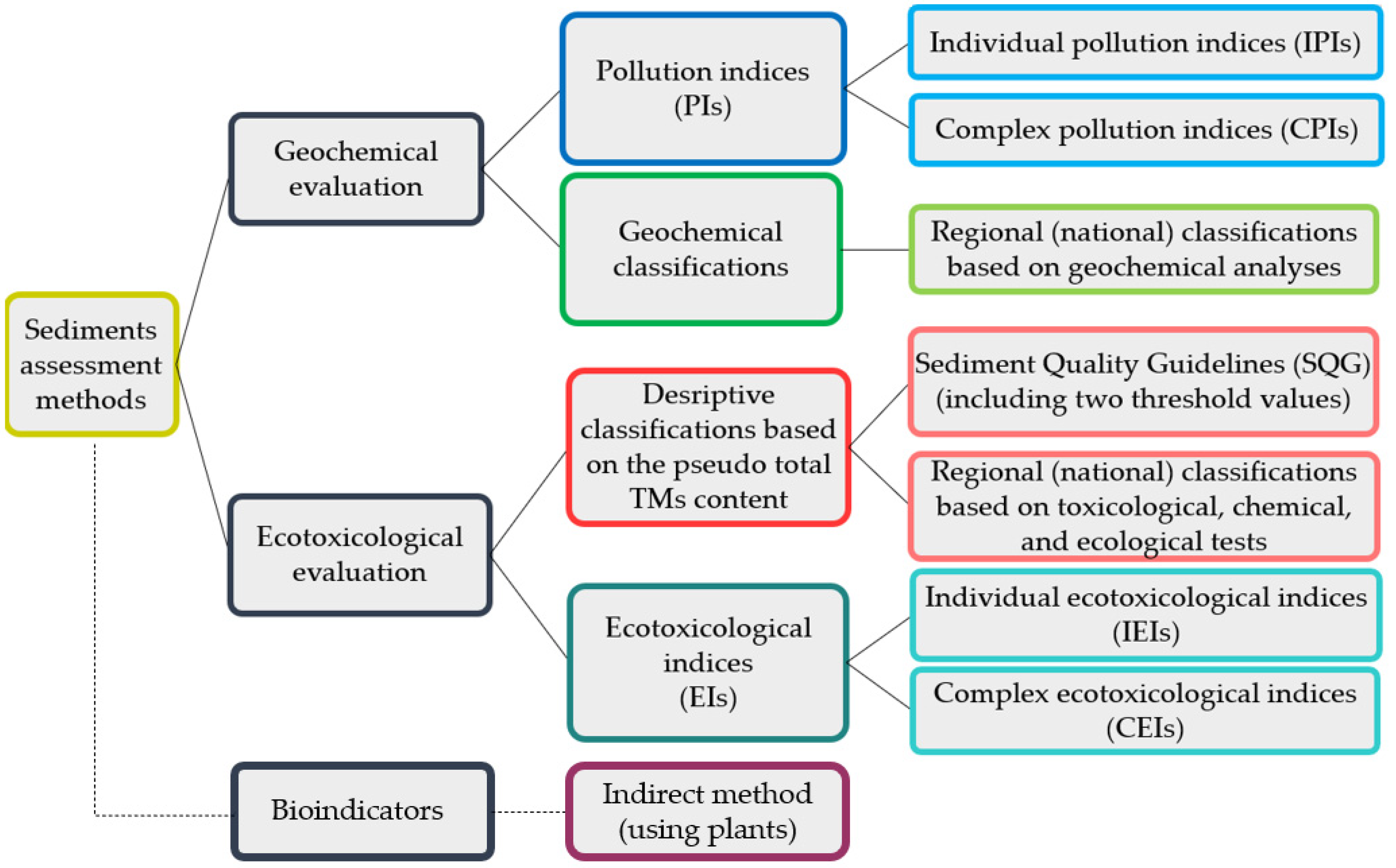
4. Assessment Techniques for Sediments Contaminated with HMs

The most effective approach in assessing sediment contamination with PTEs relies on the use of several assessment tools that can be grouped according to geochemical and ecotoxicological evaluation, as shown in Figure 1. Another method for indirect assessment of TM sediment contamination is the use of bioindicators.
Geochemical evaluation is usually based on pollution indices (PIs), while geochemical classifications are usually implemented by national governments. Both approaches rely on the establishment of a geochemical background. Among ecotoxicological methods, descriptive classifications (usually based on the ecotoxicological effect on benthic organisms—Sediment Quality Guidelines (SQG) as well as those based on toxicological, chemical, and ecological tests) and ecotoxicological indices (EIs) are used. Since the preference for adopting a sediment assessment method is usually on the side of the lawmakers, many classification and indices have been introduced since 1980.

4.1. Geochemical Evaluation

4.1.1. Geochemical Background and Geochemical Baseline

There are two controversial issues within contemporary geochemistry and environmental biochemistry: the geochemical background and the geochemical baseline of an element or chemical compound. The geochemical baseline is easier to determine—it is commonly used for assessing the environmental status before embarking on a specific investment (e.g., constructing a power plants). In exploratory geochemistry, geochemical background means the natural concentration of an element in the environment, i.e., a non-anomalous concentration of elements that corresponds to Clarke’s characteristic for their geochemical environment [20]. There are several methods to determine the accurate geochemical background. Once this value is determined, the pollution status can more precisely be assessed. These methods rely on statistical (indirect, theoretical) and empirical (direct, geochemical) determinations. An integrated approach combining both methods is also in use. Geochemical methods involve analysing samples unaffected by anthropogenic activities, which are also referred to as preindustrial samples. Usually, deep core samples and/or samples collected at a certain distance from pollution sources are used to establish geochemical background values. Statistical methods involve a determination and elimination of outliers, which are identified by standard deviation, regression analysis, or by using the Tukey boxplot method [56].
The geochemical background is not a constant value over time due to natural processes taking place at the interface of water and sediment. Additionally, the geochemical background value is local or regional rather than global. The adopted geochemical background affects the overall assessment environment quality. Sometimes, the reference level follows the shale standard (from 1961), i.e., the average content of elements in the earth’s crust [57], although this approach is incorrect.

4.1.2. Pollution Indices

According to Weissmannová and Pavlovský [6], pollution indices (PIs) can be divided into two categories including Individual (single) PIs (IPIs) and Complex (total) PIs (CPIs). In such a division, IPIs are calculated based on the contents of each metal separately in particular sediments. IPIs can be used to classify sediments into several classes according to the degree of pollution presented by a single metal. CPIs are calculated as multielement indices based on IPIs. Moreover, CPIs can be composed of IPIs separately. PIs are of most use when they meet several criteria: (1) they are easy to calculate, (2) they make reference to the geochemical background, and (3) they are widely used, which makes it possible to compare sediments from different sites.

Individual Pollution Indices (IPIs)

The IPIs used for sediment assessment are presented in Table A2 in Appendix B. In this group, five indices were identified: Contamination Factor (CF) [58], Geoaccumulation Index (Igeo) [59], Enrichment Factor (EF) [60], Pollution Index (Pi) [15,54], and Threshold Pollution Index (PIT) [28]. Each of these indices compares the concentration of a given metal in a sample ( C m S a m p l e ) to its comparative concentration—represented by C m P r e (preindustrial concentration of TM) or C m B a c k g r o u n d (geochemical background concentration of TM) [40,58,61,62,63,64].
CF is originally defined as a ratio of mean TM content averaged from at least five samples ( C m S a m p l e ) and metal concentration in preindustrial sediments [58,61,62]. According to Dung et al. [20] the ratio can also refer to background TM content. This approach is included in Pi. However, usually both indices (CF and Pi) are treated by authors interchangeably. The difference lies in the classification of the contamination levels; it also depends on whether the values of C m P r e and C m B a c k g r o u n d are consistent with each other. CF and Pi are easy to calculate, although both omit natural variability, grain-size, and reference elements ratios. Moreover, they do not take into account metal fractionation even though the formulas of the equations themselves make it possible.
Igeo proposed by Müller [59] is a commonly used index, which uses a completely different approach from other IPIs, since it defines seven classes of TM sediment contamination. The TM content in a sample is referred to as C m B a c k g r o u n d . The formula includes a constant value of 1.5, which is used to offset the natural TM fluctuations in the environment and detect minor anthropogenic impact [6].
EF is an effective tool for TM content comparison [13]. In comparison to other IPIs, EF requires the most extensive data input, such as geochemical background concentration of TM ( C m B a c k g r o u n d ) and reference element concentration in a sample ( C r e f ) as well as in the reference environment ( B r e f ). The reference element has a low occurrence variability. The reference element—and this could be Sc, Mn, Ti, Al, Fe, and Ca—has a low occurrence variability. Frequently used reference metals are Mn, Al, and Fe [12]. Usually, Fe has a relatively high natural concentration in comparison to other metals and is therefore not expected to be enriched from anthropogenic sources [64]. The use of EF seeks to reduce the metal variability associated with the granulometric composition (mud/sand ratios). The EF could be also expressed as a percentage.
PIT is based on the single Pollution Index (Pi), which refers the TM content in a sample to the tolerance levels of metal concentration ( C T L ).   C T L could be established by national guidelines or criteria regarding health-threatening TM content [63]. The determination of the threshold parameter ( C T L ) is freeform and can be adjusted to the state of the environment and defined individually by national regulations. Therefore, this index may be an effective tool in the hands of environmental managers.
All of the described IPIs omit the metal fractionation and mobility/bioavailability. IPIs are usually calculated in accordance with total metal content; however, they can be easily applied in calculations that include fractionation (as described in Section 4.3).

Complex Pollution Indices (CPIs)

A list of CPIs is presented in Appendix C. CPIs mostly rely on CF or Pi values for TMs under analysis. Thus, the starting point for a comprehensive metal contamination assessment is IPI analysis. Table A3 in Appendix C presents calculation formulas with classifications and descriptions (pros and cons considered by the authors) for the following CPIs: Pollution Load Index (PLI) [62], Contamination Degree (CDeg) [58], Modified Contamination Degree (mCDeg) [64], Sum of Pollution index (PIsum) [63], Average of Pollution Index (PIAvg) [63], Weighted average of Pollution Index (PIwAvg) [58,59,63], Background Enrichment Factor = New Pollution Index (PIN) [65], Product of Pollution Index (PIProd) [63], Weighted power product of Pollution Index (PIwpProd) [63], Vector modulus of Pollution Index (PIvectorM) [63], Nemerow Pollution Index (PINemerow) [66], Integrated Pollution Index (IntPI) [67], and Metallic Pollution Index (MPI) [68,69].
PLI is a very easy-to-use index based on CF values specified for a selected number of metals. Moreover, the deterioration of site quality could be straightforwardly specified because the unity value of PLI (PLI = 1) is the boundary differentiating the adverse impact on the quality of sediments from non-polluted sites [62]. The overarching merit is a comprehensive assessment of sediments, while the disadvantages are related to the shortcomings of the CF index.
CDeg and mCDeg are also based on CF values for analysed TMs. The difference lies in the classification of sediment contamination status. CDeg defines sediment contamination referring to four categories, while mCDeg distinguishes seven ranges of sediment quality [58,64].
The equations for calculating PIsum and PIAvg are similar to those for CDeg and mCDeg. The difference lies in the use of individual Pi (Pi = SPI = PI) factors related to C m B a c k g r o u n d (not to C m P r e ) [63]. In order to evaluate the sediments with PIsum, it is necessary to specify the classification scale for each individual case. The defined scale should refer to the number of selected TMs used to assess contamination. The pollution evaluation with PIAvg is easy to apply due to the reference to unity (1). PIwAvg application when the TM weight is equal to unity ( w i = 1 ) is a special form of PIsum.
PIN is based on Pi (Pi = SPI = PI) and requires the TM class to be determined (from 1 to 5 in reference to Pi). This very precise scale classifies sediments into five categories [68].
PIProd is a Cartesian product of Pi applied for a selected number of metals. The classification should be powered by n (count of TMs) to determine the contamination of sediments [63]. PIwpProd uses the weight of Pi in an equation, which is similar to those used for calculating PIProd [63]. PIvectorM was introduced by Gong et al. [63] and depends on Pi and the number of TMs selected for investigation. PINemerow determination emphasises the maximum value of a single Pollution Index (Pi) for all TMs; however, it does not include the weight of Pi [66]. IntPI is an easy-to-calculate index based on the Pi mean value. The classification based on IntPI divides sediment contamination into low, moderate, and strong [67,70].
MPI is equal to PLI. The general difference lies in C m B a c k g r o u n d used in the equation for the Pi calculations [71].
In relation to CPIs, one major advantage is the possibility to comprehensibly evaluate the effects of several metals simultaneously. The authors of this review believe that the the Pi weight, which represents the impact of an individual metal on the overall sediment pollution rating, plays a significant role in the calculations. This approach is used by PIwAvg and PIwpProd. Moreover, it would seem to be more accurate to include the maximum Pi as a reference in the calculations of PINemerow. Despite the mentioned advantages of PIwAvg, PIwpProd, and PINemerow, it is still desirable to use simpler calculations, which are included by PLI, CDeg, mCDeg, PIsum, etc.—due to their simplicity and frequent use in different studies.

4.1.3. Geochemical Classifications Referring to the Geochemical Background

Extensive environmental monitoring is required to develop geochemical classification and a database. Often, such studies end by mapping a given area to present geochemical data as accurately as possible [72]. Since determining the geochemical background is usually a fundamental step while assessing the environmental status of a given site, such classifications have a temporary value [20].
In Poland, the first attempts to classify lake and river sediments contaminated with TMs were made by Bojakowska and Sokołowska [73]. This so-called “geochemical classification of aquatic sediments” approach involves standardising samples, taking into account a grain size smaller than 0.2 mm. Moreover, this classification applies to samples digested with hydrochloric acid, nitric acid, or aqua regia. The geochemical criteria distinguish four geochemical quality classes presented and described in Table 1. This classification was developed in 1998, so the geochemical background could have changed since then. However, it is still used in Poland in the absence of other regulations. In Table 1, the geochemical quality classes are collated with geochemical background values established using different approaches. Depending on the goals, TM contents in analysed sediments can be compared with preindustrial concentrations [58], trace metal content in world soils [74], or shale standard [57].

4.2. Ecotoxicological Evaluation

In order to assess the level of contamination that is still safe for living organisms, it is necessary to apply ecotoxicological criteria or use indicators that take into account the level of metal toxicity.

4.2.1. Descriptive Classifications Based on Total TM Content

Internationally, a range of sediment quality guidelines (SQGs) have been proposed for contaminants. Originally, they provided the information on SQGs compared with a reference or background concentration of analysed substances [76]. After the 1980s, SQGs were developed to evaluate sediment quality where harm to aquatic organisms and the environment was observed [77]. In general, SQG approaches that use different criteria and factors are divided into two main categories [76]:
-
Empirically based SQGs—relying on the empirical relationships needed to determine the sediment contamination level at which a toxic response occurs; these are frequently used for TMs and As.
-
Theoretically based SQGs—relying on the parameters that describe the bioavailability of contaminants (equilibrium partitioning, EqP); these are mainly used for organic compounds (less often for TMs).
Both types of SQG predict adverse ecological effects caused by sediment contamination by the response of benthic organisms. SQGs feature two concentration thresholds: the first below which adverse effects are not expected to occur (threshold effect concentration—TEC) and the second above which adverse effects are expected to occur more often than not (probable effect concentration—PEC). The limitation of this approach is that it leaves significant uncertainty in the “grey” area of contaminant concentrations that lie between TEC and PEC. Therefore, it may be necessary to perform a site-specific analysis. Another relevant issue in the case of SQGs is that these descriptions apply to only one type of contaminant, which may lead to inaccurate conclusions in the contamination description, as the sediments are a sink for various type of contaminants that can contribute to their overall toxicity. Table 2 outlines the most popular empirical SQGs used in practice. All of them are based on differently described terms of TEC and PEC (e.g., TEL/PEL, ERL/ERM, or LEL/SEL) [78,79,80]. Moreover, we presented the average TEC and PEC values calculated based on the literature (TEClit and PEClit).
In parallel with the intense work undertaken on SQGs in North America and Australia, several approaches and descriptive classifications and recommendations were also developed in Europe. It is worth noting that the authorities and legislators usually consider water quality as a priority, paying less attention to the state of sediments. It should be emphasised that contaminants accumulated for decades in the bottom sediments of water bodies could be released into the water column and cause its recontamination, thereby directly affecting water quality. Despite the large-scale processes that can affect the stability of sediments, there are different inceptors of secondary water recontamination, such as pH fluctuation, or the disturbance of sediment structure during dredging operations or boat movement.
In Germany, the Länder-Arbeitsgemeinschaft Wasser classification (LAWA) [83] is used to assess Hg, Cd, Zn, Pb, Cu, Cr, and Ni content in water, suspended solids, and sediments. The LAWA classification is constrained to the methodology of digestion with the use of aqua regia. This approach does not allow silicates to dissolve; therefore, the term “pseudo total” concentration of TMs is used in the literature. However, in terms of the actual contamination status of sediments and their impact on the aquatic environment, the mobile and unstable forms of TMs are most relevant [75]. In the light of this, digestion by using aqua regia or diluted acids (e.g., hydrochloric acid, nitric acid) may determine the bioavailable fraction of TMs that take part in environmental processes, while it remains impossible to determine the content of TMs bound in minerals resistant to weathering processes. LAWA classification divides sediments into seven classes of contamination, depending on the TM contents in aquatic ecosystems. The boundary values for each class are presented in Table 3.
Following the LAWA classification, Ahlf et al. [84] introduced guidelines for evaluating sediment quality based on integrated toxicological, chemical, and ecological approaches (hereafter referred to as modified LAWA). This approach is based on a series of three different tests that should be performed step-by-step, starting from an ecotoxicological assessment. If the ecotoxicological test confirms sediment contamination, the second step is introduced, which focuses on chemical analyses. The final assessment stage involves an additional and thorough analysis of factors that may harm the environment. The classification of TM sediment contamination applied by Ahlf et al. [84] (Table 3) combines temporary valuation standards of river mud and ATV standards concerning sewage and garbage. The final evaluation is based on the concentration limits for class II, which constitutes a point of reference.
In accordance with the Water Framework Directive, water and sediment quality assessment considers the extent of deviation from reference conditions with no or with very minor anthropogenic influence. The general conclusion from analyses of sediments guidelines is that they have advantages as well as limitations for their application in sediment quality assessment [85].

4.2.2. Ecotoxicological Indices (EIs)

EIs as indicators of ecotoxicology comprise numerous indices, such as Ecological Risk Factor (ER= Eri = Risk Index (RI)) [58]—the only IEI, Contamination Severity Index (CSI) [86], Sediment Pollution Index (SPI) [58,64], Risk Assessment Code (RAC) [35], Risk Index (PERI) [87,88], and the probability of Toxicity Index (MERMQ) [86]. The list of IEIs and CEIs are presented in Table A4 Appendix D with classification and a summary of strengths and weaknesses.
ER describes the ecological risk caused by TM. T r i in the ER formula represents the toxic-response factor for a given metal, and so this index ties the risk assessment with the metal content in a sample [6]. SPI also refers to T r i of TMs and additionally takes into account the average shale concentration of TMs. Moreover, SPI is tailored for the comprehensive evaluation of several elements at the same time. Another difference between ER and SPI lies in diverse points of reference—ER classification refers to ecological risk, and SPI refers to the sediment pollution level. PERI is a complex index based on a single ER. The toxic response factors for TMs according to Håkanson [58] are as follows: Hg—40, Cd—30, As—10, Cu—5, Pb—5, Cr—2, and Zn—1. T r i in the limnic system was discussed and established by Håkanson according to the “abundance principle” of elements in different matrixes. The element with the highest mean concentration must be ranked as 1.0; according to this assumption, analysed elements were marked with the following abundance number: Zn = 1 < Cu = 3.4 < Pb = 13 < Cr = 110 < As = 140 < Cd = 230 < Hg = 1160. Note that the abundance number is not equal to the toxic factor. Håkanson corrected the abundance number to reflect the “sink-effect”. This effect is related to different footprints caused by substances (e.g., Cr has the lowest sink-factor = 2, which implies that this element leaves the heaviest footprint in the sediment, while Hg has the highest sink-factor =320, which means that much more Hg can be found in water compared to sediments). Taking into account the dimension problem, Håkanson corrected the abundance numbers that correspond to T r i . Moreover, according to Kabata-Pendias and Pendias [58], the highest T r i corresponds to strong chemical and biological activity in the case of Hg and high solubility in acidic environments and mobility for Cd. Quite low T r i for Pb is related to its low mobility. T r i = 2 for Cr is related to the principle that only Cr(VI) is toxic; at the same time, Cr(VI) is easily reduced to poorly soluble Cr(III), which is generally difficult for plants and benthic organisms to absorb [58].
CSI requires the use of computed weight of each TM according to Pejman et al. [86]: (Cu—0.075, Zn—0.075, Cr—0.134, Ni—0.215, Pb—0.251, Cd—0.25). The weight of TMs may result from statistical analyses (e.g., Principal Component Analyses—PCAs and/or Factor Analyses—FAs). Moreover, CSI requires the application of ERL and ERM, and at the same time, it is highly accurate and could provide a precise evaluation of sediments.
RAC depends on exchangeable and carbonate fractions determination (determined with CH3COOH 0.11 M solution) [35]. The classification refers to the percentage of mobile fractions in relation to the total concentration of bound TMs in all fractions together. It is worth noting that RAC is the sole index that combines the speciation analyses of TMs. Therefore, it is very valuable for evaluating the mobility and bioavailability of metals.
MERMQ is also referred to in the literature as a combined effect of Toxic Metals (mPECQ). This complex EI is based on TM content in the sample and the second threshold level of effects (e.g., ERM for MERMQ and PEC for mPECQ) [86].

4.3. Extended Sediments Quality Ranking

4.3.1. Integrated Geoaccumulation Index—Igeointegrated

The approach described by Von Tümpling et al. in 2013 [89] relies on Igeo introduced by Müller [59], and this index is combined with metal speciation analysis based on BCR (Community Bureau of Reference) three-stage sequential extraction—this approach is referred to as “extended use of Igeo in combination with BCR fractionation”. To compare the results obtained with Igeointegrated between fractions, an integrated Igeo was introduced (ΣIgeointegrated). The sum of Igeointegrated offers a general overview of the contamination degree of the considered elements in one fraction in comparison to ΣIgeointegrated of other fractions. The ΣIgeointegrated equation is as follows:
I g e o i n t e g r a t e d = j = 1 m k = 1 n m j , k
where m is the quality class, j is the sampling point (SP), and k is the element. The geoaccumulation classes (described in Table A2 Appendix B) of all the examined TMs are added for each fraction. If there is no contamination or no accumulation of an investigated element, the resulting sum is 0. The maximum class is 6.
The Igeointegrated approach can completely change the result of the sediment assessment based on the total TM content performed by Igeo. The results reported by Von Tümpling et al. [89] for Klinke River in Germany indicated that F3, F2, and F1 had the greatest ΣIgeointegrated. At the same time, the ‘‘good chemical status’’ classification in accordance with total TM content was overturned by the sequential extraction method, which demonstrated that changes in element speciation can lead to higher TM mobility, which may increase the hazardous potential of sediments.

4.3.2. Fractionation of TMs

In order to establish how TMs behave in the sediment–water or soil–water environments, the presence of physical and chemical forms of metals—i.e., fractionation, also called speciation—must be determined. Therefore, speciation is an identification of various physicochemical forms of elements in the analysed material and/or mutual proportions of these forms. This approach helps to understand the mobility of metals in the environment, although the sample processing is time consuming [90].
The analytical methods for the chemical section of TMs in the solid phase involve single reagent leaching, sequential extractions, and ion exchange resins [55]. In general, the processes involving the separation of different species are based on selective chemical reactions and/or extraction procedures (e.g., liquid–liquid, solid-phase extraction). The final result of element contents is presented in mg/kg and or mg/L (ppm—parts per million) or ng/kg and/or ng/L (ppb—parts per billion). Therefore, the overall process is complex, arduous, and susceptible to critical errors that are sometimes neglected. In the field of geochemistry, sequential extraction has proven its value. Nevertheless, accuracy at every stage of sample processing and analysis is crucial to guarantee an acceptable level for detecting (LOD—limit of detection) and quantifying the analytes [91]. TMs may be determined by commonly used instruments such as flame (FAAS), hydride generation (HGAAS), and electrometry (ETAAS) atomic absorption spectrometry, as well as inductively coupled plasma mass spectrometry (ICP-MS) and emission spectrometry (ICP-OES). In comparison with procedures in which total TM contents are determined in a direct manner, the extraction methods generate more uncertainties. This inconvenience is caused by difficulties in isolating compounds from substrates, upsetting the equilibrium between different chemical species, insufficient analytical sensitivity, or a lack of certified reference materials [92].
Many selective extraction methods have been developed, among others, by Tessier et al. [93], Boszke [94], Miller et al. [95], and Fiedler et al. [21]. One method that seeks to minimise errors during sample processing and analysis was proposed by the European Community Bureau of Reference—the BCR method [96].
The BCR three-step extraction procedure is similar to those proposed by Tessier et al. [90]. The key difference involves combining the first fraction of the procedure (instead of evaluating the exchangeable and carbonate fractions separately, the BCR procedure combines both); therefore, BCR distinguishes four factions (F1—exchangeable, F2—reducible, F3—oxidisable, and F4—residual). The description of subsequent steps of the BCR extraction procedure is presented in Table 4.

4.4. Bioindicators

In recent decades, the interest in using bioindicators as monitoring tools to examine environmental pollution caused by TMs has been growing steadily. Numerous plants are used as bioindicators to construct assumptions regarding environmental conditions. In this context, plants including macrophytes can be used as bioindicators for TM-related environmental pollution due to their ability to absorb metals from air, water, sediment, soil, and the food chain [97]. In general, bioindicators are characterised by the following abilities: they are easy to grow and cultivate, can withstand polluted environments, and can accumulate high pollutant concentration in their biomass; they are ecologically and economically important for society, and they should be abundant and widespread. In addition, bioindicators not only provide sediment, soil, and water remediation but are also a feasible tool for the recovery of valuable elements to develop a circular economy [98]. In practice, aquatic and related fauna, microbial systems, fungi, animals, and plants are popular targets of TM monitoring programs used as bioindicators to formulate conclusions regarding the environmental contamination status. Biological indicators provide information on the long-term impact of TM contamination [97]. There are many reasons to use a given species as bioindicators, while the key issue lies in the correlation of analysed toxic compounds/elements between species and contaminated matrix (as waters, sediments, or soils) [99].
In this review, different bioindicator plant species were identified from different studies based on their survival, highest metal accumulation, and biomass production in different polluted environments (soil and water) (Table 5). Moreover, metals such as Zn, Cd, Cu, and Ni were predominantly investigated in most regions. For instance, Salinitro et al. [100] depicted the linear relation of Ni in soils and in Poa annua shoots (R2 = 0.78) and Senecio vulgaris (R2 = 0.88). Therefore, these species have been demonstrated to be reliable indicators of both total and bioavailable Ni fractions in an anthropogenic environment. Extensive research on bioindicators in an estuarine and coastal environment was performed by Farias et al. [98]. In this study, Ulva australis, Zostera muelleri, and Ruppia megacarpa were selected for bioindicator identification due to their great abundance and the highest content of TMs inside their tissues. These species were verified as potential bioindicators of TM (As, Cu, Pb, and Zn) pollution in estuary sediments.
Some authors also focused on highly toxic elements such as Hg and As. These non-essential elements are uptaken passively by plants [24]. Many plant species presented tolerance to As contamination, as presented by Singh et al. [101] based on the example of Vetiveria zizanoides, which demonstrated resistance to As stress and feasibility for revegetation/remediation of As-contaminated soils. Although Hg in plants has no metabolic function, it could be easily translocated from roots and rhizomes to shoots [102].
High resistance to changes in salinity, fertility, textures, and pH is presented by an extensively distributed species Phragmites australis [103]. Ganjali et al. [104] demonstrated that Phragmites roots can be used as bioindicators of Fe, Cu, Cd, and Ni.
Phragmites and Salix species were studied widely for the phytoremediation of TMs in temperate and boreal climates. Salix schwerinii and S. myrsinifolia are known as bioindicators in boreal climates. In addition, hybrid cultivars of Salix, such as Klara (Salix viminalis × S. schwerinii × S. dasyclados) and/or Karin (S. viminalis × S. schwerinii) are in use in bioindication. Salam et al. [105] proved that Klara (Salix viminalis × S. schwerinii × S. dasyclados) accumulated high concentrations of Cu, Zn, and Ni in leaves, shoots, and roots from soils. At the same time, Klara may be considered for phytostabilisation and rhizofiltration due to the highest TM accumulation in the roots. Phragmites is an emergent plant worldwide that has demonstrated high TMs phytostabilisation properties [106,107]. In three reviewed papers, the authors focused on rare earth elements (lanthanide) such as Pr, Nd, Tb, Sm, Dy, and Er. Mikołajczyk et al. [108] have thoroughly documented the potential of Artemisia vulgaris, Papaver rhoeas, and Taraxacum officinale for phytoextraction of rare earth elements whose occurrence is increasing due to the development of modern technologies.
Bioindicator use in biomonitoring programs may be an effective approach, although each time, it requires extended research to recognise how metals in a potential bioindicator correlate with the evaluated matrix (water, sediments, or soils). Species properties regarding metal uptake, the antagonistic and synergistic properties between the elements as well as whether the metal is essential or non-essential play a key role in evaluating bioindication technology [23]. Nevertheless, this is a useful assessment tool, offering the additional potential for recovering valuable elements, and so it is expected to develop relatively soon.

5. Conclusions

By applying geochemical and ecotoxicological assessment and classification indices, a numeric evaluation may be obtained regarding the extent of sediment contamination. An analysis of the results yielded by recent studies using the Web of Science Core Collection (based on five keywords: sediments, trace metals, contamination, pollution indices, urban) shows that the following occur most often: (1) the researchers studied metal concentration in the surface layer of sediments (0–2 cm, 0–5 cm, 0–10 cm); (2) the most frequently used geochemical indices were Igeo, EF, and CF; (3) ecotoxicological evaluation was mainly performed by using SQG and PERI, which includes the toxic response index. The above-presented indices and classifications summarise the geochemical and ecotoxicological approaches of sediment assessment. The geoaccumulation indices help to determine whether the accumulation of TMs is due to natural processes or anthropogenic interference. Ecotoxicological assessment supports the overall contamination assessment of sediments and its harm for living organisms. The final results can be calculated for individual elements (CF, Igeo, EF, Pi (SPI), PTT) and by using complex pollution indices (PLI, Cdeg, mCdeg, Pisum, PIAvg, PIaAvg, PIN, PIProd, PIapProd, PIvectorM, PINemerow, IntPI, and MPI) for a larger set of TMs. Similar approaches can be applied for ecotoxicological indices (individual: ERi and complex: CSI, SPI, RAC, PERI, and MERMQ).
Geochemical indicators largely refer to the total metal content in the sample, although the inclusion of mobile and bioavailable fractions would appear to be indispensable for geochemical and ecotoxicological assessment. The use of Igeointegrated may help comprehensively verify the sediment quality. This approach includes contamination analysis, taking into account metal fractionation. A “good quality assessment” of sediments via Igeo may turn out to be worse after checking TM fractionation and referring to Igeointegrated (especially when a large proportion of TMs are bound in mobile or water-soluble fractions). Conversely, when TMs are mainly bound to an immobile and/or residual fraction, the Igeo assessment may be mendacious, resulting in an overestimation of the pollution level.
Bioindication is an indirect method of environmental assessment, which can support environmental quality assessment monitoring programs. Nowadays, the simultaneous use of different classifications and indices reflects a more accurate assessment of TM pollution. The most recognised bioindicators include Phragmites and Salix for TM phytoremediation, particularly Zn, Cd, Cu, and Ni in a boreal and temperate climate. Hybrid cultivars of Salix such as Klara (Salix viminalis × S. schwerinii × S. dasyclados) and Karin (S. viminalis × S. schwerinii) are also applied in biomonitoring and considered for phytostabilisation and rhizofiltration. Vetiveria zizanoides demonstrated resistance to As. Rare earth elements (lanthanides) such as Pr, Nd, Tb, Sm, Dy, and Er constitute a separate group of analysed metals investigated in plant research. This issue is of serious concern for the recovery of valuable elements in the development of a circular economy. Artemisia vulgaris, Papaver rhoeas, and Taraxacum officinale present lanthanide phytoextraction potential.
In order to be properly managed or remediated, sediments must be comprehensively evaluated. Monitoring programs for sediments in urban retention systems are crucial in this regard. A promising evaluation method is the use of bioindicators, which also have the potential to recover valuable elements. Therefore, future research should focus on developing this tool while evaluating the quality of sediments.

Author Contributions

Conceptualisation, N.N. and E.W.; methodology, N.N.; investigation, N.N., M.M., S.K.; resources, N.N.; data curation, N.N.; writing—original draft preparation, N.N. and E.W.; writing—review and editing, N.N. and E.W.; visualisation, N.N.; supervision, E.W., S.R., A.P.; funding acquisition, N.N. and E.W. All authors have read and agreed to the published version of the manuscript.

Funding

The authors acknowledge the support provided by InterPhD2 program funded by the European Union (Project No. POWR.03.02.00-IP.08–00-DOK/16).

Conflicts of Interest

The authors declare no conflict of interest.

Appendix A

Table A1. Comparison of trace elements investigated in bottom sediments of diverse urban water bodies (river, lakes, receivers, retention tanks, etc.) with concentration ranges in mg/kg d.w., indication of indices used for pollution evaluation, classifications, and verification of health risks and an indication of the use of metal fractionation.
AuthorsLocationUseAnalysed HMsTMs Ranges [mg/kg d.w.]SamplingIndicesSQGHeath RiskChemical Speciation Analysis
Sun et al., 2018 [28]Songhua River, Jilin City (China)Urban area with petrochemical industriesFive elements:
Cr, Ni, Cu, Zn, Pb
Total HMs content:
123.98–346.34
Surface sediment (0–5 cm)Igeo, PERI, RAC +
Vieira et al., 2019 [29]Arthur Thomas Lake, Londrina (Brazil)Urban lake; strongly agroindustrial economy (with coffee production)27 elements:
Na, K, Mg, Ca, Sr, Ba, Sc, La, Th, Ti, V, Cr, Mo, Mn, Fe, Co, Ni, Ag, Au, Al, Ga, P, As, Sb, Bi, S, Se
Na (1–3), K (10–30), Mg (50–290), Ca (90–570), Sr (5.00–32.0), Ba (37–180), Sc (19.4–57.1), La (14.0–35.0), Th (3.20–5.90), Ti (220–950), V (323–1331), Cr (74.0–185), Mo (0.30–1.00), Mn (640–174.-3), Fe (8940–16830), Co (19.70–62.30), Ni (18.5–63.6), Ag (0.01–3.20), Au (0.50–247.1), Ga (17.0–28.0), P (50–170), As (1.30–3.50), Sb (0.10–0.70), Bi (0.00–0.60), S (10–180), Se (0.01–1.40) Sediment cores
(0–90 cm)
EF, Igeo+
Kumar et al., 2020 [30]Yamuna River, Chambal River, Gulf of Mannar, Ganges River, Betwa River, Ken River, Beas River, Gomti River, and Gangotri River (India)Review of different TMs from sediment samples from Indian rivers’10 elements:
Cr, Mn, Fe, Co, Ni, Cu, Zn, Cd, Pb, As
Cr (0.075–2628.3), Mn (0.097–2436.5), Fe (4.23–2312.44), Co (1.10–624), Ni (0.01–1813), Cu (0.019–5214), Zn (0.13–2759), Cd (0.015–272), Pb (0.17–1297), As (0.12–197)No dataCF, EF, Igeo, PERI (=MRI), RI HI, HQ
Cui et al., 2019 [31]Harbin City, Song (China) Urban and rural rivers:Majiagou River (urban section, industrial zone) Yunliang River (rural section)Six elements:
Cr, Ni, Cu, Zn, Cd, Pb
Urban river: Cr (75.12–203.15), Ni (7.91–30.38), Cu (4.00–82.54), Zn (128.17–1416.71), Cd (0.08–4.08), Pb (8.86–57.49)
Rural river: Cr (53.65–81.92), Ni (BDL *–13.11), Cu (15.75–22.29), Zn (113.23–2474.05), Cd (BDL–4.29), Pb (9.31–114.42)
Surface sediment CF (=Pi), PINemerow, RI
Liu et al., 2020 [32]Pearl River Estuary, Xixiang River, Gongle Chung, Gushu Chung, Nanchang Chung, Tiegang reservoir flood discharge river, and Southern Airport drainage river (China) Urban areaSix elements:
Cr, Ni, Cu, Zn, Hg, Pb
Cr (35–510), Ni (15.0–194), Cu (38,0–1600), Zn (105–2600), Hg (0.009–0.85), Pb (22.9–160)Surface sediment Igeo, RI
Chassiot et al., 2019 [33]Saint-Charles River, Lake St. Charles (Canada)Upstream an urban reservoir; urban area with diverse industries 14 samples:
V, Cr, Mo, Mn, Co, Ni, Cu, Ag, Zn, Cd, Hg, Sn, Pb, As
No data of rangesSediment cores and surface sediment EF, Igeo, MPI
Hanfi et al., 2020 [34]Sediment samples around the world: Europe (Europe), Asia (Asia), Africa (Africa), North America (North America)Review of different TMs from sediment samples around the world (including 41 research paper reported between 1980 and 2018)Six elements:
Cr, Ni, Cu, Zn, Cd, Pb
Cr (29–196Europe; 0.85–144Asia; 1.4–85.7Africa; 17.1–125North America), Ni (35–128.45Europe; 12–126Asia; 1.9–67Africa; 18.1–26.5North America), Cu (73–466.9Europe; 10.99–269Asia; 11.3–243Africa; 15–356North America), Zn (125–1166Europe; 50.6–2377Asia; 13.1–1840Africa; 59–1811North America), Cd (0.2–4.6Europe; 0.12–72Asia; 0.33–6.9Africa; 0.1–8North America), Pb (48–1880Europe; 13.3–2582.5Asia; 11.2–737Africa; 10.9–2583North America)Surface sedimentCF (=Pi), Igeo
Xia et al., 2020 [35]Caohai Wetland (China)
The natural area of black-necked crane habitats in the Caohai wetlandNine elements:
Be, V, Cr, Ni, Cu, Zn, Cd, Hg, Pb
Be (0.83–2.19), V (49.1–103.1), Cr (83.5–145.9), Ni (40.3–65.7), Cu (13.5–30.9), Zn (108.9–365.4), Cd (0.5–7.34), Hg (0.30–1.34), Pb (37.3–76)Surface sediment
(0–10 cm)
EF, Igeo, PERI, RAC
Dhamodharan et at., 2019 [36]Cooum River, Chennai, (India)Urban area10 elements:
Cr, Mn, Fe, Ni, Cu, Zn, Cd, Hg, Pb, As
Cr (7.12–155), Mn (139–2167), Fe (17,389–49,568), Ni (3.54–53.1), Cu (12.3–59.39), Zn (19.7–438), Cd (0.7–24.4), Hg (0.01–0.79), Pb (0–30.6), As (45–497)Surface sediment Igeo, EF, CF, PLI, PERI
Siddiqui and Pandey, 2019 [37]Ganga River (China)Urban areaEight elements:
Cr, Mn, Fe, Ni, Cu, Zn, Cd, Pb
Cr (7.12–155), Mn (139–2167), Fe (17,389–49,568), Ni (3.54–53.1), Cu (2.1–73.98), Zn (6.3–104.3), Cd (0.21–3.6), Pb (2.1–36.5)Surface sediment (0–10 cm) CF, EF, Eri, Igeo, mCd, MPI, PERI, PI+
Hafijur Rahaman Khan et al., 2020 [38]Ganges-Brahmaputra-Meghna (Bangladesh)Bengal Basin river system19 elements:
Sc, Th, U, Hf, Nb, Ta, W, Cr, Mo, Co, Ni, Cu, Cd, Ga, In, Tl, Ge, Pb, Bi
Sc (7.93–16.79), Th (13.28–29.51), U (2.5–4.71), Hf (3.31– 12.50), Nb (11.75– 17.68), Ta (1.08–1.58), W (1.46–2.90), Cr (43.48–120.61), Mo (0.12–0.72), Co (9.99–19.81), Ni (19.20–85.80), Cu (11.70–48.96), Cd (0.02–0.17), Ga (13.48–23.48), In (0.01–0.09), Tl (0.12–1.04), Ge (1.33–1.63), Pb (19.63–28.78), Bi (0.14–0.88)Surface sedimentCF, EF, Igeo, PLI
Dević et al., 2020 [39]Belgrade (Serbia)Urban area of New Belgrade; Sava River and reservoirs for diesel fuel and mazut; high traffic zone10 elements:
V, Cr, Mn, Fe, Co, Ni, Cu, Zn, Cd, Pb
V (49.9–299.9), Cr (37–150.9), Mn (395–925), Fe (17,400–32,400), Co (15.99–36.99), Ni (50–139.9), Cu (5.5–30.9), Zn (1–615), Cd (1–4), Pb (20–190)Sediment cores and surface sediment Igeo, PERI, PLI, PINemerow
Wang et al., 2019 [40]Mid-channel of the Wen-Rui Tang River and its tributaries (China)Rural–urban areaFive elements:
Cr, Cu, Zn, Cd, Pb
Average: Cr (248 ± 131), Cu (995 ± 2011), Zn (2345 ± 2901), Cd (62 ± 125), Pb (217 ± 226) Surface sediment
(0–10 cm)
Eri, PERI, RAC+
Cui et al., 2020 [41]Dongfenggou River, Miaotaigou River, Huaijiagou River, Harbin (China)Suburban riversSix elements:
Cr, Ni, Cu, Zn, Cd, Pb
Cr (64.0–180.6), Ni (11.8–106.4), Cu (14.6–182.5), Zn (175.8–1198.8), Cd (0.3–3.8), Pb (16.8–150.6)Surface sediments PLI, RI
Barhoumi et al., 2019 [42]Someşu Mic River (Romania)Different human activities around, e.g., industries, urban, and agricultureEight elements:
Cr, Mn, Fe, Ni, Cu, Zn, Cd, Pb
Cr (9.39–43.15), Mn (159.90–4707.21), Fe (11,359–35,661.28), Ni (14.73–47.69), Cu (7.22–65.56), Zn (42.12–236.82), Cd (0.04–0.35), Pb (12.27–131.39)Surface sediment (0–20 cm) EF, Igeo, Romanian legislation+
Nodefarahani et al., 2020 [43]Namak Lake (Iran)Seasonal lake
nourished by surface run-off and groundwater resources
Nine elements:
V, Cr, Mn, Fe, Ni, Cu, Zn, Al., Pb
V (0.55–3.19), Cr (0.507–1.83), Mn (5.1–34.1), Fe (195.6–1117), Ni (0.239–1.209), Cu (0.57–1.3), Zn (0.346–1.225), Al (1.140–1.903), Pb (0.15–1.16)Surface sediment Igeo, EF, mPECQ+
Nargis et al., 2018 [44]River Buriganga (Bangladesh)Most of the industries and/or factories, such as tanneries, metal goods manufacturing, electroplating, batteries, shipyard, are located on the banks of the river15 elements:
Ba, U, V, Cr, Mo, Mn, Ni, Cu, Zn, Cd, Hg, As, Bi, Se, Pb
Ba (20.80 ± 2.21M **; 23.09 ± 2.63W ***), U (0.45 ± 0.09M; 0.50 ± 0.11W), V (7.51 ± 2.25M; 8.66 ± 2.77W), Cr (39.70 ± 18.84M; 41.45 ± 15.88W), Mo (0.40 ± 0.09M; 0.44 ± 0.11W), Mn (37.58 ± 3.13M; 39.06 ± 2.72W), Ni (6.39 ± 0.96M; 7.14 ± 1.11W), Cu (14.07 ± 15.93M; 15.93 ± 18.38W), Zn (36.73 ± 34.38M; 40.71 ± 37.33W), Cd (0.21 ± 0.02M; 0.23 ± 0.03W), Hg (0.016 ± 0.001M; 0.018 ± 0.001W), As (0.18 ± 0.12M; 0.21 ± 0.13W), Bi (0.33 ± 0.02M; 0.36 ± 0.02W), Se (1.07 ± 0.05M; 1.19 ± 0.05W), Pb (10.41 ± 13.61M; 11.40 ± 15.09W)Surface sediment (0–5 cm)Cdeg, CF, Eri, PLI, PERI
Xia et al., 2020 [45]Wuhan (China)20 lakes along a rural to the urban gradient in central China11 elements:
Cr, Mn, Fe, Co, Ni, Cu, Zn, Cd, Pb, Al, As
Cr (111.35 ± 43.93RRG ****; 95.50 ± 4.89RCFG *****; 111.29 ± 36.18UPG ******; 99.78 ± 8.47UCFG *******), Mn (970 ± 640RRG; 420 ± 140RCFG; 590 ± 100UPG; 710 ± 160 UCFG), Fe (37,570 ± 12,660RRG; 38,640 ± 3110RCFG; 38,260 ± 3010UPG; 39,900 ± 3080 UCFG), Co (19.81 ± 7.54RRG; 15.93 ± 1.40RCFG; 14.12 ± 1.37UPG; 16.63 ± 1.09 UCFG), Ni (32.10 ± 9.24RRG; 43.67 ± 4.25RCFG; 40.47 ± 3.30UPG; 44.61 ± 3.50 UCFG), Cu (105.45 ± 113.98RRG; 37.37 ± 5.47RCFG; 93.72 ± 74.94UPG; 62.65 ± 35.21 UCFG), Zn (105.75 ± 43.16RRG; 95.97 ± 13.15RCFG; 166.71 ± 4.71UPG; 134.41 ± 37.27 UCFG), Cd (0.50 ± 0.16RRG; 0.32 ± 0.06RCFG; 0.61 ± 0.16UPG; 0.45 ± 0.11 UCFG), Pb (32.59 ± 6.55RRG; 29.51 ± 2.15RCFG; 62.87 ± 27.83UPG; 39.06 ± 11.88 UCFG), Al (25,770 ± 15,580RRG; 23,600 ± 9400RCFG; 45,500 ± 3290UPG; 33,760 ± 16,500 UCFG), As (6.53 ± 1.89RRG; 10.04 ± 1.05RCFG; 10.69 ± 0.85UPG; 11.15 ± 1.49 UCFG)Surface sediment (0–5 cm)EF, RI
Wojciechowska et al., 2019 [46]Gdansk (Poland)Bottom sediments of urban retention tanksSix elements:
Cr, Ni, Cu, Zn, Cd, Pb
Cr (2.43–25.8), Ni (3.76–11.03), Cu (3.04–1133), Zn (17.9–362), Cd (0.088–0.60), Pb (5.77–162)Surface sediment (0–5 cm) CF, Igeo, LAWA, PLI, RI, HQ
Nawrot et al., 2020 [47]Gdansk (Poland)Bottom sediments of urban retention tanksSix elements:
Cr, Fe, Ni, Cu, Zn, Cd, Pb
Cr (2.45–74.5), Fe (3993–63,817), Ni (1.57–25.8), Cu (3.24–119), Zn (12.5–584), Cd (0.003–0.716), Pb (4.91–309)Sediment coresAF, EF, mCdeg +
Jaskuła et al., 2021 [48]Warta River (Poland)Bottom sediments of the third longest river in PolandSix elements:
Cr, Ni, Cu, Zn, Cd, Pb
Cr (0.78–193), Ni (0.56–36.7), Cu (0.40–116), Zn (0.50–519), Cd (0.03–14.5), Pb (1.0–144)Surface sediment (0–5 cm)EF, Igeo, MPI, PLI+
Kostka and Leśniak, 2021 [49]Wigry Lake (Poland) * WLBottom sediments Seven elements:
Cr, Mn, Fe, Cu, Zn, Cd, Pb
Cr (0.20–22.61), Mn (18–1698), Fe (80–32,857), Cu (0.02–59.7), Zn (3.1–632.1), Cd (0.003–3.060), Pb (7.0–107.5) Surface sediment (0–5 cm) SQG+
Ribbe et al., 2021 [50]Lake Victoria, Ugandan part (Uganda)Bottom sediments of the largest tropical lake in the worldSeven elements:
Cr, Ni, Cu, Zn, Cd, Pb, As
Cr (29–100), Ni (19–56), Cu (21–121), Zn (49–103), Cd (0.06–0.26), Pb (10–25), As (2.9–6.6)Surface sediment (the upper 15 cm)Igeo, LAWA +
Xiao et al., 2021 [51]Lijiang River, Guilin City (China)Analysis of a 160 km section of the river10 elements:
Cr, Mn, Co, Ni, Cu, Zn, Cd, Hg, Pb, As
Cr (24.38–95.38), Mn (176.25–1572.50), Co (4.50–15.38), Ni (11.63–37.13), Cu (9.38–102.75), Zn (53.63–258.0), Cd (0.16–4.41), Hg (0.08–2.13), Pb (17.88–171.75), As (9.97–36.44)Surface sediment
(0–5 cm)
Igeo, mCdeg, RI
Castro et al., 2021 [52]San Luis River (Argentina)Bottom sedimentsNine elements:
Cr, Mn, Co, Ni, Cu, Zn, Cd, Pb, As
Cr (0.5–32), Mn (10–420), Co (0.5–14), Ni (1–19), Cu (0.5–70), Zn (0–600), Cd (0–1,5), Pb (0–45), As (0.5–18)Surface sediment
(0–2 cm)
CF, EF, Igeo+
Explanations: * BDL—below detection limit; ** M—in monsoon; *** W—in winter; **** RCFG—rural commercial fishing group; ***** RRG—rural reservoir group; ****** UPG—urban park group; ******* UCFG—urban commercial fishing group * WL Wigry Lake in Poland is located in Wigry National Park (non urban area)—just to comparison with other studies.

Appendix B

Table A2. A list of Individual (single) Pollution Indices (IPIs) given in the literature with classification and a basic description of strengths and weaknesses.
IndexFormulaClassificationDescription (Pros “+” and Cons “–“)References
Contamination Factor (CF) C F = C m S a m p l e   C m P r e
C m S a m p l e —TM content
*   C m P r e —preindustrial concentration of TM
CF < 1—low,
1 ≤ CF < 3—moderate,
3 ≤ CF < 6—considerable,
CF ≥ 6—very high
+
dedicated to individual metal
+
simple in use (easy to calculate)
+
comparing the sample to the reference contamination status of analysed element (pre-industrial)
omits the TM availability and mobility in the environment
omits the natural variability process, grain-size, and reference elements ratios
[58]
Geoaccumulation Index (Igeo) I g e o = log 2 [ C m S a m p l e 1.5 × C m B a c k g r o u n d ]
C m S a m p l e —TM content
C m B a c k g r o u n d —geochemical background concentration of TM
Class 0: Igeo ≤ 0—uncontaminated,
Class 1: 0 < Igeo ≤ 1—uncontaminated to moderately contaminated,
Class 2: 1 < Igeo ≤ 2—moderately contaminated,
Class 3: 2 < Igeo ≤ 3—moderately to strongly contaminated,
Class 4: 3 < Igeo ≤ 4—strongly contaminated,
Class 5: 4 < Igeo ≤ 5—strongly to extremely contaminated,
Class 6: Igeo > 5—extremely contaminated
+
dedicated to individual metal
+
simple in use (easy to calculate)
+
comparing the sample to the background contamination status of analysed element
+
1.5 multiplication factor reduces the possible variation of lithogenic effects
+
precise scale
+
widely used
omits the TM availability and mobility in the environment
omits the natural variability process, grain-size, and reference elements
incorrect selection of Background leads to mistaken results
[59]
Enrichment Factor (EF) E F = C m S a m p l e C r e f C m B a c k g r o u n d B r e f
C m S a m p l e —TM content
C m B a c k g r o u n d —geochemical background concentration of TM
C r e f —concentration of the reference TM in analysed sample
B r e f —reference TM concentration in the reference environment
EF < 1—no enrichment,
1 ≤ EF < 3—minor enrichment,
3 ≤ EF < 5—moderate enrichment,
5 ≤ EF < 10—moderately severe enrichment,
10 ≤ EF < 25—severe enrichment,
25 ≤ EF < 50—very severe enrichment,
EF ≥ 50—ultra-high enrichment
+
dedicated to individual metal
+
simple in use (easy to calculate)
+
comparing the sample to the reference contamination status of analysed element and to the normalise element (e.g., Al or Fe) as well as to reference content of analysed TM and normalise element
+
estimate the anthropogenic impact at all the possibility of contamination assessment of several TMs in reference to normalise element
+
precise scale
+
widely used
omits the TM availability and mobility in the environment
omits the natural variability process, grain-size
incorrect selection of reference value leads to mistaken results
[60]
Pollution Index (Pi) = Single Pollution Index (SPI) P i = S P I = P I = C m S a m p l e C m B a c k g r o u n d
C m S a m p l e —TM content
C m B a c k g r o u n d —geochemical background concentration of TM
Pi < 1—unpolluted, low level of pollution
1 ≤ Pi ≤ 3—moderate polluted
3 > Pi—strong polluted
+
dedicated to individual metal
+
simple in use (easy to calculate)
+
comparing the sample to the background contamination status of analysed element
+/−
similar to CF
omits the TM availability and mobility in the environment
omits the natural variability process, grain size, and reference elements ratios
[15,54]
Threshold Pollution Index (PIT) P I T = C m S a m p l e C T L
C m S a m p l e TM content
C T L —tolerance levels of metal concentration;
PIT < 1—unpolluted
1 ≤ PIT ≤ 2—low polluted
2 ≤ PIT ≤ 3—moderate polluted
3 ≤ PIT ≤ 5—strong polluted
5 ≤ PIT—very strong polluted
+
dedicated to individual metal
+
simple in use (easy to calculate)
+
comparing the sample to the tolerance level of metal concentration (which could be assumed as a comparative value before assessment)
+/−
freedom in determining the threshold parameter (CTL) (which can be matched with stringent pollution determination regulations)
+/−
similar to CF
omits the TM availability and mobility in the environment
omits the natural variability process, grain size, and reference elements ratios
[28]
* Preindustrial concentration of TM according to Håkanson [58] [mg/kg]: Hg—0.25, Cd—1.0, As—15, Cu—50, Pb—70, Cr—90, Zn—175.

Appendix C

Table A3. A list of Complex Pollution Indices (CPIs) given in the literature with classification and basic description of strengths and weaknesses.
IndexFormulaClassificationDescription (Pros “+” and Cons “–“)References
Pollution Load Index (PLI) P L I = C F 1 · C F 2 · C F 3 · · C F i n
C F i —Contamination Factor of i element
n—the number of analysed TMs
PLI < 1—not polluted
PLI = 1—baseline levels of pollution
PLI > 1—polluted
+
allows for identifying the contamination in relation to several trace metals
+
easy to apply (easy to calculate)
+
widely used
+
gives the comprehensive screen of sediment sample
+
allows comparing samples taken from different locations
+
used CF (includes C m P r e )*
omits the TM availability and mobility in the environment
omits the natural variability process, grain size, and reference elements ratios
incorrect selection of C m P r e value could lead to mistaken results
[62]
Degree of contamination (Cdeg) C d e g = i = 1 n C F i
C F i Contamination Factor of i element
n—the number of analysed TMs
C d e g < 8—low degree of contamination
8     C d e g   < 16—moderate degree of contamination
16 C d e g   < 32—considerable degree of contamination
C d e g   ≥ 32—very high degree of contamination
+
allows for identifying the contamination in relation to several trace metals
+
easy to apply (easy to calculate)
+
precise scale
+
assesses a sum of contamination factors
+
used CF (includes C m P r e ) *
not widely used
does not include geochemical background
the preindustrial reference value is necessary
omits the TMs availability and mobility in the environment
omits the natural variability process, grain size, and reference elements ratios
[58]
Modified contamination factor (mCdeg) m C d e g = 1 n · i = 1 n C F i
C F i Contamination Factor of i element
n—the number of analysed TMs
m C d e g   < 1.5—very low
1.5     m C d e g   < 2—low
2     m C d e g   < 4—moderate
4     m C d e g   < 8—high
8     m C d e g   < 16—very high
16     m C d e g     < 32—extremely high
m C d e g   ≥ 32—ultra-high
+
allows for identifying the contamination in relation to several trace metals
+
easy to apply (easy to calculate)
+
precise scale
+
assesses a sum of contamination factors
+
used CF (includes C m P r e ) *
+
widely used
does not include geochemical background
the preindustrial reference value is necessary
omits the TMs availability and mobility in the environment
omits the natural variability process, grain size, and reference elements ratios
[64]
Sum of Pollution Index (PIsum) P I s u m = i = 1 n P i
P i —calculated value for Pollution Index
n—the number of analysed TMs
The classification for Pi can be used in PIsum.
The values in PIsum should be multiplied by n (count of TMs):
PIsum < 1n—unpolluted, low level of pollution
1nPIsum ≤ 3n—moderately polluted
3n < PIsum—heavily polluted
+
defined as the sum of all determined contents of TMs, expressed as Pi
+
dedicated to combining all analysed TMs
+
based on Pi (includes C m B a c k g r o u n d )
does not require the variation of natural processes
omits the TMs availability and mobility in the environment
the key is the choice of appropriate C m B a c k g r o u n d value
does not include precise scale
[63]
Average of Pollution Index (PIAvg) P I A v g = 1 n · i = 1 n P i
P i —calculated value for Pollution Index
n—the number of analysed TMs
P I A v g values in excess of 1.0 show a lower quality of the sediments, which is conditioned by high contamination and low quality
+
allows for identifying the contamination in relation to several trace metals
+
based on Pi (includes C m B a c k g r o u n d )
+
easy to apply (easy to calculate)
+
lack of threshold for maximum values
does not require the variation of natural processes
omits the TMs availability and mobility in the environment
the key is the choice of appropriate C m B a c k g r o u n d value
does not include precise scale
[63]
Weighted Average of Pollution Index (PIwAvg) P I w A v g = i = 1 n w i · P i
P i —calculated value for Pollution Index
w i weight of P i
n—the number of analysed TMs
When   P I w A v g is used with the Σwi = 1 condition, terminologies can also be used as single indices (the classification for Pi can be applied)
+
dedicated to combining all analysed TMs
+
based on Pi (includes C m B a c k g r o u n d )
does not include precise scale
require to establish the weight of P i values for each TM
the condition Σwi = 1 is not necessary, so the “average” is just for the sake of meaning in terminology
[58,59,63]
Background enrichment factor = New Pollution Index (PIN) P I N = i = 1 n W i 2 · P i
P i —calculated value for Pollution Index
W i class of TM considering degree of contamination (from 1 to 5 basing on Pi)
n—the number of analysed TMs
0 ≤ PIN < 7—
clean7 ≤ PIN < 95.1—trace contaminant
95.1 ≤ PIN < 518.1—lightly contaminant
518.1 ≤ PIN < 2548.5—contaminant
PIN ≥ 2548.8—high contaminant
+
dedicated to integrating contamination into a single value
+
based on Pi (includes C m B a c k g r o u n d )
+
precise scale
not widely used
omits the TMs availability and mobility in the environment
requires the computation of Wi
[65]
Product of Pollution Index (PIProd) P I P r o d = i = 1 n P i
P i —calculated value for Pollution Index
n—the number of analysed TMs
The classification for Pi can be used in PIProd.
The values in PIProd should be powered by n (count of TMs):
PIProd< 1n—unpolluted, low level of pollution
1nPIProd≤ 3n—moderately polluted
3n< PIProd—heavily polluted
+
defined as the product of all determining contents of TMs, expressed as Pi
+
dedicated to combining all analysed TMs
+
based on Pi (includes C m B a c k g r o u n d )
does not require the variation of natural processes
omits the TMs availability and mobility in the environment
the key is choice of appropriate C m B a c k g r o u n d value
does not include precise scale
not widely used
[63]
Weighted power product of Pollution Index (PIwpProd) P I w p P r o d = i = 1 n P i w i
P i —calculated value for Pollution Index
w i weight of P i
n—the number of analysed TMs
When   P I w p P r o d is used with the Σwi = 1 condition, terminologies can also be used as single indices (the classification for Pi can be applied)
+
dedicated to combine all analysed TMs
+
based on Pi (includes C m B a c k g r o u n d )
does not include precise scale
require to establish the weight of P i values for each TM
the condition Σwi = 1 is not necessary
[63]
Vector modulus of Pollution Index (PIvectorM) P I v e c t o r M = 1 n · i = 1 n P i 2
P i —calculated value for Pollution Index
n—the number of analysed TMs
Not specified
+
easy to apply (easy to calculate)
+
application of C m B a c k g r o u n d
+
based on Pi
+
dedicated to combine all contaminations in one index
not specified scale
not widely used (not much described in the literature)
does not require the variation of natural processes
[63]
Nemerow Pollution Index (PINemerow) P I N e m e r o w = ( 1 n · i = 1 n P i ) 2 + P i m a x 2     2  
P i —calculated value for Pollution Index
P i m a x —the maximum value of the single pollution indices of all TMs
n—the number of analysed TMs
PINem < 0.7—safety domain
0.7≤ PINem < 1—precaution domain
1≤ PINem w< 2—slightly polluted domain
2≤ PINem < 3—moderately polluted domain
PINem > 3—seriously polluted
+
reflects the sediment environmental pollution
+
emphasize the maximum value of the single Pi of all TMs
+
precise scale
+
dedicated to combine all analysed TMs with reference to the maximum value of the single Pi
does not include weight of P i values
needs to rank elements
[66]
Integrated Pollution Index (IntPI) I n t P I = m e a n ( P i i )
P i —calculated value for Pollution Index
IPI < 1—low contaminated
1 ≤ IPI ≤ 2—moderately contaminated
IPI < 2—heavily contaminated
+
easy to apply (easy to calculate)
+
application of C m B a c k g r o u n d
+
based on Pi
not widely used
does not require the variation of natural processes
[67]
Metallic Pollution Index (MPI) M P I = ( P i 1 · P i 2 · · P i n ) 1 / n
P i —calculated value for Pollution Index
n—the number of analysed TMs
MPI > 1—indicate pollution
MPI < 1—indicate no pollution
+
similar to PLI
+
basing on Pi values
+
gives the comprehensive screen of sediment sample
+
allows to compare samples taken from different locations
omits the TM availability and mobility in the environment
omits the natural variability process, grain size, and reference elements ratios
[68,69]
* ( includes   C m P r e )—with reference to the literature, the CPIs are related to the IPI, but it should be noted that in the IPI C m P r e   and   C m B a c k g r o u n d are two different concepts that are often confused/or taken interchangeably.

Appendix D

Table A4. A list of ecotoxicological indices (EIs) given in the literature with classification and basic description of strengths and weaknesses.
IndexFormulaClassificationDescription (Pros “+” and Cons “–“)References
Individual Ecotoxicological Index (IEI)
Ecological Risk Factor (ER, Eri) Risk Index (RI) E R i = T r i · C F i
*   T r   i – toxic-response factor for a given element “i”
C F i —contamination factor for a given element “i”;
ERi < 40—low potential ecological risk;
40≤ ERi < 80—moderate potential ecological risk;
80≤ ERi < 160—considerable potential ecological risk;
160 ≤ ERi < 320—high potential ecological risk;
ERi ≥ 320—very high ecological risk
+
dedicated to the toxicity of individual metals
+
simple in use (easy to calculate)
+
uses CF values
omits the TM availability and mobility in the environment
omits the natural variability process, grain size, and reference elements ratios
[58]
Complex Ecotoxicological Index (CEI)
Contamination Severity Index (CSI) C S I = i = 1 n w · ( ( C m S a m p l e E R L ) 1 2 + ( C m S a m p l e E R M ) 2 )
w —the computed weight of each TM according to Pejman et al. [86] **
C m S a m p l e TM content
E R L —Effects Range-Low according to Table 2
E R M —Effects Range-Median
according to Table 2
w = ( l o a d i n g   v a l u e i · e i g e n   v a l u e ) i = 1 n ( l o a d i n g   v a l u e i · e i g e n   v a l u e )
l o a d i n g   v a l u e i   and   e i g e n   v a l u e —determined with the use of PCA/FA
CSI < 0.5—uncontaminated
0.5 ≤ CSI < 1—very low severity of contamination
1 ≤ CSI < 1.5—low severity of contamination
1.5 ≤ CSI < 2—low to moderate severity of contamination
2 ≤ CSI < 2.5—moderate severity of contamination
2.5 ≤ CSI < 3—moderate to high severity of contamination
3 ≤ CSI < 4—high severity of contamination
4 ≤ CSI < 5—very high severity of contamination
5 ≤ CSI—ultra-high severity of contamination
+
helpful in determining the limit of toxicity above which adverse impacts on the sediment environment are observed
+
precise scale
+
dedicated to combining all contaminations in one index
+
includes adverse biological effects
not widely used
needs the ERL and ERM values
requires the w values of each TM, which should be calculated using PCA/FA with considered the factors attributed to anthropogenic sources
[86]
Sediment Pollution Index (SPI) S P I = i = 1 n C m S a m p l e i C m A v e r a g e i · T r   i i = 1 n T r i
C m S a m p l e TM content in a sample
C m A v e r a g e —average shale concentration of TM
*   T r   i —toxic-response factor for a given element “i”
n—the number of analysed TMs
0 ≤ SPI < 2—natural sediments
2 ≤ SPI < 5— low polluted
5 ≤ SPI < 10—moderately polluted
10 ≤ SPI < 20—highly polluted
SPI > 20—dangerous sediments
+
includes the toxicity of individual metal
+
simple in use (easy to calculate)
+
combined index
+
delivers the information of diverse sites contamination
omits the TM availability and mobility in the environment
omits the natural variability process, grain size, and reference elements ratios
neglecting the changes of TM/reference element ratios based on natural processes
TM toxicity weights are available for Hg, Cd, As, Cu, Pb, Cr, and Zn
[58,64]
Risk Assessment Code (RAC)The exchangeable and carbonate fractions are determined by a single extraction with a CH3COOH 0.11 M solutionPercentage extracted by CH3COOH 0.11 M solution is compared to the following scale:
RAC ≤ 1—no risk
1 < RAC ≤ 10—low risk
11 < RAC ≤ 30—medium risk; 31 < RAC ≤ 50: very high risk
+
indicates the potential risk to the ecosystem caused by TMs bounded in fractions weakly associated in the sediments
+
Delivers real risk information
the extraction procedure is needed (time-consuming procedure)
[35]
Risk Index (PERI) P E R I = i = 1 n E R i
n—the number of analysed TMs
E R i —calculated value for Ecological Risk Factor
P E R I < 90—low
9 P E R I < 180—moderate
180 P E R I < 360—strong
360 P E R I < 720—very strong
P E R I ≥ 720—highly strong
+
comprehensive ecological risk and contamination assessment
+
includes the toxicity of analysed metals (basing on ERi)
+
simple in use (easy to calculate)
disadvantages similar to ERi
[87,88]
The probability of toxicity (MERMQ) M E R M Q = i = 1 n C m S a m p l e i E R M i n
C m S a m p l e TM content
n—the number of analysed TMs
E R M —Effects Range-Median
according to Table 2
 
This index is also found as combined effect of Toxic Metals, means (mPECQ):
m P E C Q = i = 1 n C m S a m p l e i P E C i n
C m S a m p l e TM content
n—the number of analysed TMs
P E C —probable effect concentration according to Table 2
MERMQ < 0.1—low-risk level (probability of toxicity—9%)
0.1 ≤MERMQ < 0.5—medium risk level (probability of toxicity—21%)
0.5 ≤ MERMQ < 1.5—high risk level (probability of toxicity—49%)
MERMQ > 1.5—very high-risk level (probability of toxicity—76%)
+
dedicated to combining all contaminations in one index
+
precise scale
+
helpful in determining the biological effects
+
identification of risk areas
not widely used
needs the ERM/PEC values
+
does not require the variation of natural processes
[86]
* Toxic response factor for subsequent trace metals according to Håkanson [58]: Hg—40, Cd—30, As—10, Cu—5, Pb—5, Cr—2, Zn—1. ** Weight of each heavy metal according to Pejman et al. [86]: Cu—0.075, Zn—0.075, Cr—0.134, Ni—0.215, Pb—0.251, Cd—0.25.

References

  1. Sakson, G.; Brzezinska, A.; Zawilski, M. Emission of heavy metals from an urban catchment into receiving water and possibility of its limitation on the example of Lodz city. Environ. Monit. Assess. 2018, 190, 281. [Google Scholar] [CrossRef] [PubMed] [Green Version]
  2. Zafra, C.; Temprano, J.; Tejero, I. The physical factors affecting heavy metals accumulated in the sediment deposited on road surfaces in dry weather: A review. Urban Water J. 2017, 9006, 1–11. [Google Scholar] [CrossRef]
  3. Antoniadis, V.; Shaheen, S.M.; Stärk, H.J.; Wennrich, R.; Levizou, E.; Merbach, I.; Rinklebe, J. Phytoremediation potential of twelve wild plant species for toxic elements in a contaminated soil. Environ. Int. 2021, 146, 106233. [Google Scholar] [CrossRef]
  4. Liu, L.; Luo, X.B.; Ding, L.; Luo, S.L. Application of Nanotechnology in the Removal of Heavy Metal from Water; Elsevier Inc.: New York, NY, USA, 2018; ISBN 9780128148389. [Google Scholar]
  5. Wuana, R.A.; Okieimen, F.E. Heavy metals in contaminated soils: A review of sources, chemistry, risks and best available strategies for remediation. Int. Sch. Res. Not. Ecol. 2011, 2011, 1–20. [Google Scholar] [CrossRef] [Green Version]
  6. Weissmannová, H.D.; Pavlovský, J. Indices of soil contamination by heavy metals—Methodology of calculation for pollution assessment (minireview). Environ. Monit. Assess. 2017, 189, 1–25. [Google Scholar] [CrossRef]
  7. Kowalska, J.B.; Mazurek, R.; Gąsiorek, M.; Zaleski, T. Pollution indices as useful tools for the comprehensive evaluation of the degree of soil contamination—A review. Environ. Geochem. Health 2018, 40, 1–26. [Google Scholar] [CrossRef] [Green Version]
  8. Szmagliński, J.; Nawrot, N.; Pazdro, K.; Walkusz-Miotk, J.; Wojciechowska, E. The fate and contamination of trace metals in soils exposed to a railroad used by Diesel Multiple Units: Assessment of the railroad contribution with multi-tool source tracking. Sci. Total Environ. 2021, 798, 149300. [Google Scholar] [CrossRef]
  9. Bednarova, Z.; Kuta, J.; Kohut, L.; Machat, J.; Klanova, J.; Holoubek, I.; Jarkovsky, J.; Dusek, L.; Hilscherova, K. Spatial patterns and temporal changes of heavy metal distributions in river sediments in a region with multiple pollution sources. J. Soils Sediments 2013, 13, 1257–1269. [Google Scholar] [CrossRef]
  10. Bartoli, G.; Papa, S.; Sagnella, E.; Fioretto, A. Heavy metal content in sediments along the Calore river: Relationships with physical-chemical characteristics. J. Environ. Manag. 2012, 95, S9–S14. [Google Scholar] [CrossRef] [PubMed]
  11. Monrabal-Martinez, C.; Meyn, T.; Muthanna, T.M.; Monrabal-martinez, C.; Meyn, T.; Muthanna, T.M. Characterization and temporal variation of urban runoff in a cold climate—Design implications for SuDS. Urban Water J. 2018, 16, 1–9. [Google Scholar] [CrossRef]
  12. Sekabira, K.; Origa, H.O.; Basamba, T.A.; Mutumba, G.; Kakudidi, E. Assessment of heavy metal pollution in the urban stream sediments and its tributaries. Int. J. Environ. Sci. Technol. 2010, 7, 435–446. [Google Scholar] [CrossRef] [Green Version]
  13. Murphy, L.U.; Cochrane, T.A.; O’Sullivan, A. The influence of different pavement surfaces on atmospheric copper, lead, zinc, and suspended solids attenuation and wash-off. Water Air Soil Pollut. 2015, 226, 1–14. [Google Scholar] [CrossRef]
  14. Charters, F. Characterising and Modelling Urban Runoff Quality for Improved Stormwater Management. Ph.D. Thesis, Department of Civil and Natural Resources Engineering, University of Canterbury, Christchurch, New Zealand, 2016. [Google Scholar]
  15. Nour, H.E.; El-Sorogy, A.S.; Abdel-Wahab, M.; Almadani, S.; Alfaifi, H.; Youssef, M. Assessment of sediment quality using different pollution indicators and statistical analyses, Hurghada area, Red Sea coast, Egypt. Mar. Pollut. Bull. 2018, 133, 808–813. [Google Scholar] [CrossRef] [PubMed]
  16. Walaszek, M.; Bois, P.; Laurent, J.; Lenormand, E.; Wanko, A. Urban stormwater treatment by a constructed wetland: Seasonality impacts on hydraulic efficiency, physico-chemical behavior and heavy metal occurrence. Sci. Total Environ. 2018, 637–638, 443–454. [Google Scholar] [CrossRef] [PubMed]
  17. Simpson, S.; Batley, G. Sediment Quality Assessment a Practical Guide, 2nd ed.; CSIRO Publishing: Collingwood, Australia, 2016; ISBN 9781486303847. [Google Scholar]
  18. Nawrot, N.; Wojciechowska, E.; Rezania, S.; Walkusz-Miotk, J.; Pazdro, K. The effects of urban vehicle traffic on heavy metal contamination in road sweeping waste and bottom sediments of retention tanks. Sci. Total Environ. 2020, 749, 141511. [Google Scholar] [CrossRef]
  19. USEPA. Contaminated Sediment Remediation Guidance for Hazardous Waste Sites; Official Solid Waste Emergency Response; USEPA: Washington, DC, USA, 2005; p. 236.
  20. Dung, T.T.T.; Cappuyns, V.; Swennen, R.; Phung, N.K. From geochemical background determination to pollution assessment of heavy metals in sediments and soils. Rev. Environ. Sci. Biotechnol. 2013, 12, 335–353. [Google Scholar] [CrossRef]
  21. Fiedler, H.D.; López-Sánchez, J.F.; Rubio, R.; Rauret, G.; Quevauviller, P.; Ure, A.M.; Muntau, H. Study of the stability of extractable trace metal contents in a river sediment using sequential extraction. Analyst 1994, 119, 1109–1114. [Google Scholar] [CrossRef]
  22. Bonanno, G.; Borg, J.A.; Di Martino, V. Levels of heavy metals in wetland and marine vascular plants and their biomonitoring potential: A comparative assessment. Sci. Total Environ. 2017, 576, 796–806. [Google Scholar] [CrossRef]
  23. Klink, A.; Macioł, A.; Wisłocka, M.; Krawczyk, J. Metal accumulation and distribution in the organs of Typha latifolia L. (cattail) and their potential use in bioindication. Limnologica 2013, 43, 164–168. [Google Scholar] [CrossRef]
  24. Kabata-Pendias, A.; Pendias, H. Biogeochemistry of Trace Elements; Polish Scientific Publishing Company: Warsaw, Poland, 1999; Volume 2, ISBN 0849315751. [Google Scholar]
  25. Al-Homaidan, A.A.; Al-Otaibi, T.G.; El-Sheikh, M.A.; Al-Ghanayem, A.A.; Ameen, F. Accumulation of heavy metals in a macrophyte Phragmites australis: Implications to phytoremediation in the Arabian Peninsula wadis. Environ. Monit. Assess. 2020, 192, 1–10. [Google Scholar] [CrossRef]
  26. Relić, D.; Dordević, D.; Popović, A. Assessment of the pseudo total metal content in alluvial sediments from Danube River, Serbia. Environ. Earth Sci. 2011, 63, 1303–1317. [Google Scholar] [CrossRef]
  27. Ure, A.M.; Davidson, C.M. Chemical speciation in soils and related materials by selective chemical extraction. In Chemical Speciation in the Environment, 2nd ed.; Wiley-Blackwell: Malden, MA, USA, 2007; pp. 265–300. [Google Scholar] [CrossRef]
  28. Sun, C.; Zhang, Z.; Cao, H.; Xu, M.; Xu, L. Concentrations, speciation, and ecological risk of heavy metals in the sediment of the Songhua River in an urban area with petrochemical industries. Chemosphere 2019, 219, 538–545. [Google Scholar] [CrossRef] [PubMed]
  29. Vieira, L.M.; Neto, D.M.; do Couto, E.V.; Lima, G.B.; Peron, A.P.; Halmeman, M.C.R.; Froehner, S. Contamination assessment and prediction of 27 trace elements in sediment core from an urban lake associated with land use. Environ. Monit. Assess. 2019, 191, 1–20. [Google Scholar] [CrossRef]
  30. Kumar, V.; Sharma, A.; Pandita, S.; Bhardwaj, R.; Thukral, A.K.; Cerda, A. A review of ecological risk assessment and associated health risks with heavy metals in sediment from India. Int. J. Sediment Res. 2020, 35, 516–526. [Google Scholar] [CrossRef]
  31. Cui, S.; Zhang, F.; Hu, P.; Hough, R.; Fu, Q.; Zhang, Z.; An, L.; Li, Y.F.; Li, K.; Liu, D.; et al. Heavy metals in sediment from the urban and rural rivers in Harbin City, Northeast China. Int. J. Environ. Res. Public Health 2019, 16, 4313. [Google Scholar] [CrossRef] [Green Version]
  32. Liu, C.; Yin, J.; Hu, L.; Zhang, B. Spatial distribution of heavy metals and associated risks in sediment of the urban river flowing into the Pearl River Estuary, China. Arch. Environ. Contam. Toxicol. 2020, 78, 622–630. [Google Scholar] [CrossRef]
  33. Chassiot, L.; Francus, P.; De Coninck, A.; Lajeunesse, P.; Cloutier, D.; Labarre, T. Spatial and temporal patterns of metallic pollution in Québec City, Canada: Sources and hazard assessment from reservoir sediment records. Sci. Total Environ. 2019, 673, 136–147. [Google Scholar] [CrossRef] [PubMed]
  34. Hanfi, M.Y.; Mostafa, M.Y.A.; Zhukovsky, M.V. Heavy metal contamination in urban surface sediments: Sources, distribution, contamination control, and remediation. Environ. Monit. Assess. 2020, 192, 32. [Google Scholar] [CrossRef] [PubMed]
  35. Xia, P.; Ma, L.; Sun, R.; Yang, Y.; Tang, X.; Yan, D.; Lin, T.; Zhang, Y.; Yi, Y. Evaluation of potential ecological risk, possible sources and controlling factors of heavy metals in surface sediment of Caohai Wetland, China. Sci. Total Environ. 2020, 740, 140231. [Google Scholar] [CrossRef]
  36. Dhamodharan, A.; Abinandan, S.; Aravind, U.; Ganapathy, G.P.; Shanthakumar, S. Distribution of Metal Contamination and Risk Indices Assessment of Surface Sediments from Cooum River, Chennai, India. Int. J. Environ. Res. 2019, 13, 853–860. [Google Scholar] [CrossRef]
  37. Siddiqui, E.; Pandey, J. Assessment of heavy metal pollution in water and surface sediment and evaluation of ecological risks associated with sediment contamination in the Ganga River: A basin-scale study. Environ. Sci. Pollut. Res. 2019, 26, 10926–10940. [Google Scholar] [CrossRef] [PubMed]
  38. Khan, M.H.R.; Liu, J.; Liu, S.; Li, J.; Cao, L.; Rahman, A. Anthropogenic effect on heavy metal contents in surface sediments of the Bengal Basin river system, Bangladesh. Environ. Sci. Pollut. Res. 2020, 27, 19688–19702. [Google Scholar] [CrossRef] [PubMed]
  39. Dević, G.J.; Ilić, M.V.; Zildzović, S.N.; Avdalović, J.S.; Miletić, S.B.; Bulatović, S.S.; Vrvić, M.M. Investigation of potentially toxic elements in urban sediments in Belgrade, Serbia. J. Environ. Sci. Health Part A Toxic Hazard. Subst. Environ. Eng. 2020, 55, 765–775. [Google Scholar] [CrossRef] [PubMed]
  40. Wang, Z.; Zhou, J.; Zhang, C.; Qu, L.; Mei, K.; Dahlgren, R.A.; Zhang, M.; Xia, F. A comprehensive risk assessment of metals in riverine surface sediments across the rural-urban interface of a rapidly developing watershed. Environ. Pollut. 2019, 245, 1022–1030. [Google Scholar] [CrossRef] [PubMed] [Green Version]
  41. Cui, S.; Gao, S.; Zhang, F.; Fu, Q.; Wang, M.; Liu, D.; Li, K.; Song, Z.; Chen, P. Heavy metal contamination and ecological risk in sediment from typical suburban rivers. River Res. Appl. 2020, 1–9. [Google Scholar] [CrossRef]
  42. Barhoumi, B.; Beldean-Galea, M.S.; Al-Rawabdeh, A.M.; Roba, C.; Martonos, I.M.; Bălc, R.; Kahlaoui, M.; Touil, S.; Tedetti, M.; Driss, M.R.; et al. Occurrence, distribution and ecological risk of trace metals and organic pollutants in surface sediments from a Southeastern European river (Someşu Mic River, Romania). Sci. Total Environ. 2019, 660, 660–676. [Google Scholar] [CrossRef]
  43. Nodefarahani, M.; Aradpour, S.; Noori, R.; Tang, Q.; Partani, S.; Klöve, B. Metal pollution assessment in surface sediments of Namak Lake, Iran. Environ. Sci. Pollut. Res. 2020. [Google Scholar] [CrossRef]
  44. Nargis, A.; Sultana, S.; Raihan, M.J.; Haque, M.E.; Sadique, A.B.M.R.; Sarkar, M.S.I.; Un-Nabie, M.M.; Zhai, W.; Cai, M.; Habib, A. Multielement analysis in sediments of the River Buriganga (Bangladesh): Potential ecological risk assessment. Int. J. Environ. Sci. Technol. 2019, 16, 1663–1676. [Google Scholar] [CrossRef]
  45. Xia, W.; Wang, R.; Zhu, B.; Rudstam, L.G.; Liu, Y.; Xu, Y.; Xin, W.; Chen, Y. Heavy metal gradients from rural to urban lakes in central China. Ecol. Process. 2020, 9, 1–11. [Google Scholar] [CrossRef]
  46. Wojciechowska, E.; Nawrot, N.; Walkusz-Miotk, J.; Matej-Łukowicz, K.; Pazdro, K. Heavy metals in sediments of urban streams: Contamination and health risk assessment of influencing factors. Sustainability 2019, 11, 563. [Google Scholar] [CrossRef] [Green Version]
  47. Nawrot, N.; Wojciechowska, E.; Matej-Łukowicz, K.; Walkusz-Miotk, J.; Pazdro, K. Spatial and vertical distribution analysis of heavy metals in urban retention tanks sediments: A case study of Strzyza Stream. Environ. Geochem. Health 2020, 8. [Google Scholar] [CrossRef] [PubMed] [Green Version]
  48. Jaskuła, J.; Sojka, M.; Fiedler, M.; Wróżyński, R. Analysis of spatial variability of river bottom sediment pollution with heavy metals and assessment of potential ecological hazard for the Warta river, Poland. Minerals 2021, 11, 327. [Google Scholar] [CrossRef]
  49. Kostka, A.; Leśniak, A. Natural and anthropogenic origin of metals in lacustrine sediments; assessment and consequences—A case study of Wigry lake (Poland). Minerals 2021, 11, 1–22. [Google Scholar] [CrossRef]
  50. Ribbe, N.; Arinaitwe, K.; Dadi, T.; Friese, K.; von Tümpling, W. Trace-element behaviour in sediments of Ugandan part of Lake Victoria: Results from sequential extraction and chemometrical evaluation. Environ. Earth Sci. 2021, 80, 1–14. [Google Scholar] [CrossRef]
  51. Xiao, H.; Shahab, A.; Xi, B.; Chang, Q.; You, S.; Li, J.; Sun, X.; Huang, H.; Li, X. Heavy metal pollution, ecological risk, spatial distribution, and source identification in sediments of the Lijiang River, China. Environ. Pollut. 2021, 269, 116189. [Google Scholar] [CrossRef]
  52. Castro, M.F.; Almeida, C.A.; Bazán, C.; Vidal, J.; Delfini, C.D.; Villegas, L.B. Impact of anthropogenic activities on an urban river through a comprehensive analysis of water and sediments. Environ. Sci. Pollut. Res. 2021, 28, 37754–37767. [Google Scholar] [CrossRef]
  53. HELCOM Guideline for the Determination of Heavy Metals in Sediment. 2015. Available online: https://helcom.fi/?s=Guideline+for+the+determination+of+heavy+metals+in+sediment (accessed on 12 May 2021).
  54. Mulligan, C.; Fukue, M.; Sato, Y. Sediments Contamination and Sustainable Remediation; CRC Press: Boca Raton, FL, USA, 2009; ISBN 9781420062236. [Google Scholar]
  55. Tack, F.M.G.; Verloo, M.G. Chemical speciation and fractionation in soil and sediment heavy metal analysis: A review. Int. J. Environ. Anal. Chem. 1995, 59, 225–238. [Google Scholar] [CrossRef]
  56. Gałuszka, A. A review of geochemical background concepts and an example using data from Poland. Environ. Geol. 2007, 52, 861–870. [Google Scholar] [CrossRef]
  57. Turekian, K.K.; Wedepohl, K.H. Distribution of the elements in some major units of the earth’s crust. Geol. Soc. Am. Bull. 1961, 72, 175–192. [Google Scholar] [CrossRef]
  58. Håkanson, L. An ecological risk index for aquatic pollution control.a sedimentological approach. Water Res. 1980, 14, 975–1001. [Google Scholar] [CrossRef]
  59. Müller, V.G. Pollutants in sediments—Sediments as pollutants [available in German: Schadstoffe in Sedimenten—Sedimente als Schadstoffe]. Mitt. Osterr. Geol. Ges. 1986, 79, 107–126. [Google Scholar]
  60. Sutherland, R.A. Bed sediment-associated trace metals in an urban stream, Oahu, Hawaii. Environ. Geol. 2000, 39, 611–627. [Google Scholar] [CrossRef]
  61. Tomlinson, D.L.; Wilson, J.G.; Harris, C.R.; Jeffrey, D.W. Assessment of heavy metal enrichment and degree of contamination around the copper-nickel mine in the Selebi Phikwe Region, Eastern Botswana. Environ. Ecol. Res. 2013, 1, 32–40. [Google Scholar] [CrossRef]
  62. Tomlinson, D.L.; Wilson, J.G.; Harris, C.R.; Jeffrey, D.W. Problems in the assessment of heavy-metal levels in estuaries and the formation of a pollution index. Helgol. Meeresunters. 1980, 33, 566–575. [Google Scholar] [CrossRef] [Green Version]
  63. Gong, Q.; Deng, J.; Xiang, Y.; Wang, Q.; Yang, L. Calculating pollution indices by heavy metals in ecological geochemistry assessment and a case study in parks of Beijing. J. China Univ. Geosci. 2008, 19, 230–241. [Google Scholar] [CrossRef]
  64. Abrahim, G.M.S.; Parker, R.J. Assessment of heavy metal enrichment factors and the degree of contamination in marine sediments from Tamaki Estuary, Auckland, New Zealand. Environ. Monit. Assess. 2008, 136, 227–238. [Google Scholar] [CrossRef] [PubMed]
  65. Weissmannová, H.D.; Pavlovský, J.; Chovanec, P. Heavy metal contaminations of urban soils in Ostrava, Czech Republic: Assessment of metal pollution and using Principal Component Analysis. Int. J. Environ. Res. 2015, 9, 683–696. [Google Scholar]
  66. Cheng, J.; Shi, Z.; Zhu, Y. Assessment and mapping of environmental quality in agricultural soils of Zhejiang Province, China. J. Environ. Sci. 2007, 19, 50–54. [Google Scholar] [CrossRef]
  67. Chen, T.B.; Zheng, Y.M.; Lei, M.; Huang, Z.C.; Wu, H.T.; Chen, H.; Fan, K.K.; Yu, K.; Wu, X.; Tian, Q.Z. Assessment of heavy metal pollution in surface soils of urban parks in Beijing, China. Chemosphere 2005, 60, 542–551. [Google Scholar] [CrossRef]
  68. Caeiro, S.; Costa, M.H.; Ramos, T.B.; Fernandes, F.; Silveira, N.; Coimbra, A.; Medeiros, G.; Painho, M. Assessing heavy metal contamination in Sado Estuary sediment: An index analysis approach. Ecol. Indic. 2005, 5, 151–169. [Google Scholar] [CrossRef]
  69. Gong, C.; Ma, L.; Cheng, H.; Liu, Y.; Xu, D.; Li, B.; Liu, F.; Ren, Y.; Liu, Z.; Zhao, C.; et al. Characterization of the particle size fraction associated heavy metals in tropical arable soils from Hainan Island, China. J. Geochem. Explor. 2014, 139, 109–114. [Google Scholar] [CrossRef]
  70. Lu, X.; Wang, L.; Lei, K.; Huang, J.; Zhai, Y. Contamination assessment of copper, lead, zinc, manganese and nickel in street dust of Baoji, NW China. J. Hazard. Mater. 2009, 161, 1058–1062. [Google Scholar] [CrossRef] [PubMed]
  71. Chassiot, L.; Francus, P.; De Coninck, A.; Lajeunesse, P.; Cloutier, D.; Labarre, T. Dataset for the assessment of metallic pollution in the Saint-Charles River sediments (Québec City, QC, Canada). Data Brief 2019, 26, 104256. [Google Scholar] [CrossRef] [PubMed]
  72. Guartán, J.A.; Emery, X. Regionalized classification of geochemical data with filtering of measurement noises for predictive lithological mapping. Nat. Resour. Res. 2021, 30, 1033–1052. [Google Scholar] [CrossRef]
  73. Bojakowska, I.; Sokołowska, G. Geochemical purity classes of water sediments [available in Polish: Geochemiczne klasy czystości osadów wodnych]. Przegląd Geol. 1998, 46, 49–54. [Google Scholar]
  74. Ure, A.M.; Berrow, M.L. The elemental constituents of soils. In Environmental Chemistry; Bowen, H.J.M., Ed.; Royal Society of Chemistry: London, UK, 1982; Volume 2, pp. 92–204. [Google Scholar]
  75. Lis, J.; Pasieczna, A. Geochemical Atlas of Gdańsk Region [Available in Polish: Geochemiczny Atlas Region Gdańskiego]; Wydawnictwo Kartograficzne Polskiej Agencji Ekologicznej: Warsaw, Poland, 1999. [Google Scholar]
  76. Burton, G.A. Sediment quality criteria in use around the world. Limnology 2002, 3, 65–75. [Google Scholar] [CrossRef]
  77. Wenning, R.J.; Ingersoll, C.G. Use of Sediment Quality Guidelines and Related Tools for the Assessment of Contaminated Sediments; SETAC: Pensacola, FL, USA, 2005. [Google Scholar]
  78. Smith, S.; MacDonald, D.; Keenleyside, K.; Ingersoll, C.; Field, J. A preliminary evaluation of sediment quality assessment values for freshwater ecosystems. J. Great Lakes Res. 1996, 22, 624–638. [Google Scholar] [CrossRef]
  79. Long, E.; Morgan, L. The Potential for Biological Effects of Sediment-Sorbed Contaminants Tested in the National Status and Trends Program; NOAA Technical Memorandum NOS OMA 52; National Oceanic and Atmospheric Administration: Seattle, WA, USA, 1991; p. 175. [Google Scholar]
  80. Persaud, D.; Jaagumagi, R.; Hayton, A. Guidelines for the Protection and Management of Aquatic Sediment Quality in Ontario; Water Resources Branch, Ontario Ministry of the Environment: Toronto, ON, Canada, 1993. [Google Scholar]
  81. MENVIQ. Interim Criteria for Quality Assessment of St. Lawrence River Sediment; St. Lawrence Centre and Ministère de l’Environnement du Québec: Quebec City, QC, Canada, 1992; p. 28.
  82. ANZECC; ARMCANZ. Australian and New Zealand guidelines for fresh and marine water quality. In The Guidelines Australian and New Zealand Environment and Conservation Council Agriculture and Resource Management Council of Australia and New Zealand; National Water Quality Management Strategy; Australian and New Zealand Environment and Conservation Council, Australian Water Association: Artarmon, Australia, 2000; Volume 1, p. 314. [Google Scholar]
  83. LAWA-Arbeitskreis. “Qualitative Hydrology of Rivers” Assessment of the Water Quality of Rivers in the Federal Republic of Germany [Available in German: “Zielvorgaben” in Zusammenarbeit Mit LAWA-Arbeitskreis “Qualitative Hydrologie der Fliessgewässer” Beurteilung der Wasserbeschaffenheit von Fliessgewaessern in der Bundesrepublik Deutschland]; Herausgegeben von der Länderarbeitsgemeinschaft Wasser: Berlin, Germany, 1998; ISBN 3889612245. [Google Scholar]
  84. Ahlf, W.; Hollert, H.; Neumann-Hensel, H.; Ricking, M. A guidance for the assessment and evaluation of sediment quality: A German approach based on ecotoxicological and chemical measurements. J. Soils Sediments 2002, 2, 37–42. [Google Scholar] [CrossRef]
  85. Directive 2000/60/EC of the European Parliament and of the Council of 23 October 2000 Establishing a Framework for Community Action in the Field of Water Policy; Publications Office of the European Union: Luxembourg, 23 October 2000; pp. 1–73.
  86. Pejman, A.; Bidhendi, G.N.; Ardestani, M.; Saeedi, M.; Baghvand, A. A new index for assessing heavy metals contamination in sediments: A case study. Ecol. Indic. 2015, 58, 365–373. [Google Scholar] [CrossRef]
  87. Kulbat, E.; Sokołowska, A. Methods of assessment of metal contamination in bottom sediments (case study: Straszyn Lake, Poland). Arch. Environ. Contam. Toxicol. 2019, 77, 605–618. [Google Scholar] [CrossRef] [PubMed] [Green Version]
  88. Baran, A.; Tarnawski, M.; Koniarz, T. Spatial distribution of trace elements and ecotoxicity of bottom sediments in Rybnik reservoir, Silesian-Poland. Environ. Sci. Pollut. Res. 2016, 23, 17255–17268. [Google Scholar] [CrossRef] [Green Version]
  89. Von Tümpling, W.; Scheibe, N.; Einax, J.W. Extended sediment quality rating for trace elements in urban waters—Case study Klinke, Germany. Clean Soil Air Water 2013, 41, 565–573. [Google Scholar] [CrossRef]
  90. Sutherland, R.A. BCR®-701: A review of 10-years of sequential extraction analyses. Anal. Chim. Acta 2010, 680, 10–20. [Google Scholar] [CrossRef] [PubMed]
  91. Viana, J.L.M.; Menegário, A.A.; Fostier, A.H. Preparation of environmental samples for chemical speciation of metal/metalloids: A review of extraction techniques. Talanta 2021, 226, 122119. [Google Scholar] [CrossRef] [PubMed]
  92. Kersten, M. Speciation of trace metals in sediments. In Chemical Speciation in the Environment, 2nd ed.; Ure, A.M., Davidson, C.M., Eds.; John Wiley & Sons: New York, NY, USA, 2002; pp. 301–321. [Google Scholar]
  93. Tessier, A.; Campbell, P.G.C.; Bisson, M. Sequential extraction procedure for the speciation of particulate trace metals. Anal. Chem. 1979, 51, 844–851. [Google Scholar] [CrossRef]
  94. Boszke, E. Specification of Speciation of Selected Heavy Metals (Fe, Mn, Zn, Cd, Ni, Cr, Co) in Bottom Sediments of the Baltic Sea and the Spitsbergen Region; Institute of Oceanology of the Polish Academy of Science: Sopot, Poland, 1995. (In Polish) [Google Scholar]
  95. Miller, W.P.; Martens, D.C.; Zelany, L.W. Effect of the sequence in extraction of trace metals from soils. Soil. Soil Sci. Soc. Am. J. 1986, 50, 598–601. [Google Scholar] [CrossRef]
  96. Ure, A.M.; Quevauviller, P.; Muntau, H.; Griepink, B. An account of the improvement and harmonization of extraction techniques undertaken under the auspices of the BCR of the Commission of the European Communities. Int. J. Environ. Anal. Chem. 1993, 51, 135–151. [Google Scholar] [CrossRef]
  97. Stankovic, S.; Stankovic, A.R. Bioindicators of toxic metals. In Green Materials for Energy, Products and Depollution; Springer: Amsterdam, The Netherlands, 2013; pp. 151–228. ISBN 9789400768352. [Google Scholar]
  98. Farias, D.R.; Hurd, C.L.; Eriksen, R.S.; Macleod, C.K. Macrophytes as bioindicators of heavy metal pollution in estuarine and coastal environments. Mar. Pollut. Bull. 2018, 128, 175–184. [Google Scholar] [CrossRef] [PubMed]
  99. Rayment, G.E.; Barry, G.A. Indicator tissues for heavy metal monitoring—Additional attributes. Mar. Pollut. Bull. 2000, 41, 353–358. [Google Scholar] [CrossRef]
  100. Salinitro, M.; Tassoni, A.; Casolari, S.; de Laurentiis, F.; Zappi, A.; Melucci, D. Heavy metals bioindication potential of the common weeds Senecio vulgaris L. Polygonum aviculare L. and Poa annua L. Molecules 2019, 24, 2813. [Google Scholar] [CrossRef] [Green Version]
  101. Singh, S.; Mishra, H.; Suprasanna, P. Evaluation of arsenic remediation, morphological and biochemical response by Vetiveria zizanoides L. plants grown on artificially arsenic contaminated soil: A field study. Ecol. Eng. 2021, 168, 106267. [Google Scholar] [CrossRef]
  102. Bonanno, G.; Vymazal, J. Compartmentalization of potentially hazardous elements in macrophytes: Insights into capacity and efficiency of accumulation. J. Geochem. Explor. 2017, 181, 22–30. [Google Scholar] [CrossRef]
  103. Milke, J.; Gałczyńska, M.; Wróbel, J. The Importance of biological and ecological properties of Phragmites Australis (Cav.) Trin. Ex Steud., in phytoremendiation of aquatic ecosystems—The review. Water 2020, 12, 1770. [Google Scholar] [CrossRef]
  104. Ganjali, S.; Tayebi, L.; Atabati, H.; Mortazavi, S. Phragmites australis as a heavy metal bioindicator in the Anzali wetland of Iran. Toxicol. Environ. Chem. 2014, 96, 1428–1434. [Google Scholar] [CrossRef]
  105. Salam, M.M.A.; Mohsin, M.; Pulkkinen, P.; Pelkonen, P.; Pappinen, A. Effects of soil amendments on the growth response and phytoextraction capability of a willow variety (S. viminalis × S. schwerinii × S. dasyclados) grown in contaminated soils. Ecotoxicol. Environ. Saf. 2019, 171, 753–770. [Google Scholar] [CrossRef] [PubMed]
  106. Minkina, T.; Fedorenko, G.; Nevidomskaya, D.; Fedorenko, A.; Chaplygin, V.; Mandzhieva, S. Morphological and anatomical changes of Phragmites australis Cav. due to the uptake and accumulation of heavy metals from polluted soils. Sci. Total Environ. 2018, 636, 392–401. [Google Scholar] [CrossRef] [PubMed]
  107. Nawrot, N.; Wojciechowska, E.; Pazdro, K.; Szmagliński, J.; Pempkowiak, J. Uptake, accumulation, and translocation of Zn, Cu, Pb, Cd, Ni, and Cr by P. australis seedlings in an urban dredged sediment mesocosm: Impact of seedling origin and initial trace metal content. Sci. Total Environ. 2021, 768, 144983. [Google Scholar] [CrossRef]
  108. Mikołajczak, P.; Borowiak, K.; Niedzielski, P. Phytoextraction of rare earth elements in herbaceous plant species growing close to roads. Environ. Sci. Pollut. Res. 2017, 24, 14091–14103. [Google Scholar] [CrossRef] [Green Version]
  109. You, Y.; Wang, L.; Ju, C.; Wang, G.; Ma, F.; Wang, Y.; Yang, D. Effects of arbuscular mycorrhizal fungi on the growth and toxic element uptake of Phragmites australis (Cav.) Trin. ex Steud under zinc/cadmium stress. Ecotoxicol. Environ. Saf. 2021, 213, 112023. [Google Scholar] [CrossRef]
  110. Bayouli, I.T.; Bayouli, H.T.; Dell’Oca, A.; Meers, E.; Sun, J. Ecological indicators and bioindicator plant species for biomonitoring industrial pollution: Eco-based environmental assessment. Ecol. Indic. 2021, 125, 107508. [Google Scholar] [CrossRef]
  111. Liu, C.; Liu, W.; Huot, H.; Yang, Y.; Guo, M.; Morel, J.L.; Tang, Y.; Qiu, R. Responses of ramie (Boehmeria nivea L.) to increasing rare earth element (REE) concentrations in a hydroponic system. J. Rare Earths 2021. [Google Scholar] [CrossRef]
  112. Hussain, Z.; Rasheed, F.; Tanvir, M.A.; Zafar, Z.; Rafay, M.; Mohsin, M.; Pulkkinen, P.; Ruffner, C. Increased antioxidative enzyme activity mediates the phytoaccumulation potential of Pb in four agroforestry tree species: A case study under municipal and industrial wastewater irrigation. Int. J. Phytoremediat. 2020, 23, 704–714. [Google Scholar] [CrossRef]
  113. Mohsin, M.; Kuittinen, S.; Salam, M.M.A.; Peräniemi, S.; Laine, S.; Pulkkinen, P.; Kaipiainen, E.; Vepsäläinen, J.; Pappinen, A. Chelate-assisted phytoextraction: Growth and ecophysiological responses by Salix schwerinii EL Wolf grown in artificially polluted soils. J. Geochem. Explor. 2019, 205, 106335. [Google Scholar] [CrossRef]
  114. Nworie, O.E.; Qin, J.; Lin, C. Trace element uptake by herbaceous plants from the soils at a multiple trace element-contaminated site. Toxics 2019, 7, 3. [Google Scholar] [CrossRef] [PubMed] [Green Version]
  115. Rasheed, F.; Zafar, Z.; Waseem, Z.A.; Rafay, M.; Abdullah, M.; Salam, M.M.A.; Mohsin, M.; Khan, W.R. Phytoaccumulation of Zn, Pb, and Cd in Conocarpus lancifolius irrigated with wastewater: Does physiological response influence heavy metal uptake? Int. J. Phytoremediat. 2020, 22, 287–294. [Google Scholar] [CrossRef]
  116. Kim, H.T.; Kim, J.G. Seasonal variations of metal (Cd, Pb, Mn, Cu, Zn) accumulation in a voluntary species, Salix subfragilis, in unpolluted wetlands. Sci. Total Environ. 2018, 610, 1210–1221. [Google Scholar] [CrossRef]
  117. Salam, M.M.A.; Kaipiainen, E.; Mohsin, M.; Villa, A.; Kuittinen, S.; Pulkkinen, P.; Pelkonen, P.; Mehtätalo, L.; Pappinen, A. Effects of contaminated soil on the growth performance of young Salix (Salix schwerinii EL Wolf) and the potential for phytoremediation of heavy metals. J. Environ. Manag. 2016, 183, 467–477. [Google Scholar] [CrossRef]
  118. Eid, E.M.; Shaltout, K.H. Bioaccumulation and translocation of heavy metals by nine native plant species grown at a sewage sludge dump site. Int. J. Phytoremediat. 2016, 18, 1075–1085. [Google Scholar] [CrossRef] [PubMed]
  119. Mohsin, M. Potentiality of Four Willow Varieties for Phytoremediation in a Pot Experiment. Master’s Thesis, Faculty of Science and Forestry, School of Forest Sciences, University of Eastern Finland, Kuopio, Finland, 2016. [Google Scholar]
  120. Vymazal, J. Concentration is not enough to evaluate accumulation of heavy metals and nutrients in plants. Sci. Total Environ. 2016, 544, 495–498. [Google Scholar] [CrossRef]
  121. Carpenter, D.; Boutin, C.; Allison, J.E.; Parsons, J.; Ellis, D.M. Uptake and effects of six rare earth elements (REEs) on selected native and crop species growing in contaminated soils. PLoS ONE 2015, 10, e0129936. [Google Scholar] [CrossRef] [Green Version]
  122. Ladislas, S.; El-Mufleh, A.; Gérente, C.; Chazarenc, F.; Andrès, Y.; Béchet, B. Potential of aquatic macrophytes as bioindicators of heavy metal pollution in urban stormwater runoff. Water Air Soil Pollut. 2012, 223, 877–888. [Google Scholar] [CrossRef]
Figure 1. Division of the methods of assessment of sediment contamination with PTEs.
Minerals 11 00872 g001
Table 1. The concentration of various trace metals (TMs) in mg/kg d.w. for each class of sediments—geochemical classification of aquatic sediments [57,58,73,74,75].
Trace Metal Geochemical Background [in mg/kg d.w.]Geochemical Quality Classes
PreindustrialWorld SoilsShale StandardGdansk Region Sediments (Poland)Sediments (Poland)IIIIIIIV
[58][74][57][75][73][73][73][73][73]
As-1.513-<5<10<20<50≥50
Cd1.00.620.30.51<1<3.5<6≥6
Cr90849075<50<100<400≥400
Cu5025.84556<40<100<200≥200
Pb7029.2201110<50<200<500≥500
Hg0.25-0.4-≤0.05<0.1<0.5<1.0≥1.0
Ni-33.76845<30<50<100≥100
Zn17559.8954148<200<1000<2000≥2000
Bold—geochemical quality classes description according to Bojakowska and Sokołowska: Class I—uncontaminated sediments (boundary value of elements concentration determined as from 5 to 10 times higher than the geochemical background); Class II—moderately contaminated sediments (TMs content from 10 to 20 times higher than the geochemical background); Class III—contaminated sediments (TMs content from 20 to 100 times higher than the geochemical background); Class IV—highly contaminated sediments [73].
Table 2. Sediment quality guidelines (SEQs) for TMs and metalloid in mg/kg d.w. that reflect threshold effect concentration (TEC) and probable effect concentration (PEC) [77,78,79,80,81,82].
ElementEmpirical SQGs with TEC and PEC in mg/kg·d.w.
Smith et al. [78]Long and Morgan [79]Persaud et al. [80]MENVIQ [81]ANZECC/ARMCANZ [82]Average Values Based on the Literature
TELPELERLERMLELSELMETTETSQGVSQGV-HighTEClitPEClit
As5.917338563371720701444
Cd0.5963.53590.6100.931.5101.727
Cr37.3908014526110551008037056163
Cu35.7197703901611028866527043211
Pb3591.33511031250421705022039168
Hg0.1740.4860.151.30.220.210.151.00.171
Ni183630501675356121522455
Zn123315120270120820150540200410143471
Limitations for empirical SQGs:
Advantages(1) Allows for thresholds prediction at which a toxic response of benthic organisms is probable
(2) A useful tool that allows making the first guess on the sediment contamination problem
(3) Quite simple to use with a large database of lab and field tests
Disadvantages(1) The assessment of risk and possible negative outcomes associated with toxic concentration levels, which require a separate risk evaluation
(2) “Grey” area between thresholds test errors
(3) Difficult to apply in a context of contaminant mixtures
(4) Relatively expensive research and development of new SQGs
(5) The availability of SQGs guidelines criteria and documentation is limited
TEC—Threshold-Effects Concentration; PEC—Probable-Effects Concentration; TEL—Threshold-Effects Level; PEL—Probable-Effects Level; ERL—Effects Range: Low; ERM—Effects Range: Median; MET—Minimal Effect Threshold; TET—Toxic Effect Threshold; SQGV—Sediment Quality Guideline Value; ANZECC/ARMCANZ [82]—currently used classification in Australia and New Zealand.
Table 3. The concentration of various trace metals (TMs) in mg/kg d.w. for each class of sediments—classification LAWA and modified LAWA [83,84].
ClassificationTrace Metal [in mg/kg d.w.]Contamination Class
II–IIII *II–IIIIIIIII–IVIV
LAWA [83]Cd≤0.3≤0.6≤1.2≤2.4≤4.8≤9.6>9.6
Cr≤80≤90≤100≤200≤400≤800>800
Cu≤20≤40≤60≤120≤240≤480>480
Pb≤25≤50≤100≤200≤400≤800>800
Hg≤0.2≤0.4≤0.8≤1.6≤3.2≤6.4>6.4
Ni≤30≤40≤50≤100≤200≤400>400
Zn≤100≤150≤200≤400≤800≤1600>1600
Modified LAWA [84]As3–5<10<20<40< 70<100>100
Cd0.2–0.4<0.5<1.2<5< 10<25>25
Cr60–80<90<100<150< 250<500>500
Cu20–30<40<60<150<250<500>500
Pb25–30<50<100<150<250<500>500
Hg0.2–0.4<0.5<0.8<5<10<25>25
Ni10–30<40<50<150<250<500>500
Zn90–110<150<200<500<1000<2000>2000
* Quality goal—Class II. Class I refers to uncontaminated sediment; Class I–II—sediments unpolluted or with very small anthropogenic interference; Class II corresponds to moderately polluted sediments, and it is a reference for the other levels of pollution; Class II–III—twice as much as Class II—defines moderate to significant contamination of sediments; Class III—four times more than Class II—defines significant pollution; Class III–IV—eight times more than Class II—refers to very strong pollution; Class IV—means more than eight times exceeding Class II—ultimate pollution. Comparative value is the average contents of TM expressed in mg/kg [83,84].
Table 4. The BCR three-steps sequential extraction scheme [90].
Extraction StepFractionOperational DefinitionChemical Reagents/Conditions
1F1Acid extractable (water and acid soluble)Acetic acid: CH3COOH (0.11 mol/L); pH 2.85
2F2Reducible (Fe/Mn oxides)Hydroxyloammonium chloride: NH2OH · HCl (0.1 mol/L), pH 2.0
3F3Oxidisable (organic substance and sulphides)Hydrogen peroxide: H2O2 (8.8 mol/L) followed by ammonium acetate: CH3COONH4 (1.0 mol/L), pH 2.0
4F4Residual (remaining, non-silicate bound metals)Acid digestion (e.g., Aqua regia: 3 HCl + HNO3 or HF + HNO3)
Table 5. A list of plant species tested as candidates for bioindication across the world.
Plant Species/CultivarsClimate/RegionAnalysed PollutantsTrialSourceReference
Phragmites australisTemperate/ChinaZn and CdPot experimentHydroponic[109]
Atraclytis seratuloides, Lygeum spartum, and Gymnocarpos decanderMediterranean/TunisiaCr, Co, Zn, PbFieldSoil, cement site[110]
Phragmites australisTemperate/PolandCr, Ni, Cu, Zn, Cd, PbPot experimentSediment[107]
Vetiveria zizanoidesTropical/IndiaAsFieldSoil[101]
Alopecurus pratensis, Elytrigia repens, Poa angustifolia, Holcus lanatus, Arrhenatherum elatius, Bromus inermis Leyss, Artemisia vulgaris, Urtica dioica, Achillea millefolium, Galium mollugo, Stellaria holostea, and Silene vulgarisTemperate/GermanyCr, Ni, Cu, Zn, Cd, Pb, As Pot experiment (cold-house)Soil[3]
Boehmeria nivea Sc, Y, La, Ce, Pr, Nd, Sm, Eu, Gd, Tb, Dy, Ho, Er, Tm, Yb, and LuGrowth chamberHydroponic[111]
Morus alba, Acacia nilotica, Acacia ampliceps, and Azadirachta indicaTropical/PakistanPbGreenhouseMunicipal and industrial wastewater[112]
Salix schweriniiBoreal/FinlandNi, Cu, and ZnGrowth chamberSoil[113]
Senecio vulgaris, Polygonum aviculare, and Poa annuaMediterranean/ItalyCr, Cu, Zn, Cd, and PbFieldSoil[100]
Klara (S. viminalis × S. schwerinii × S. dasyclados)Boreal/FinlandNi, Cu, and ZnPot experiment (greenhouse)Soil[105]
Artemisia vulgaris
Phalaris arundinacea
Heracleum sphondylium
Bistorta officinalis
Temperate/UKMn, Zn, and As
Mn and Ni
Cr and Zn
Mn and Zn
FieldSoil[114]
Conocarpus lancifoliusTemperate/PakistanZn, Cd, and PbPot experiment (greenhouse)Soil[115]
Salix subfragilisTemperate/KoreaMn, Cu, Zn, Cd, and PbField trialSediment (wetland)[116]
Ruppia megacarpa, Zostera muelleri, and Ulva australisTemperate-desert/AustraliaCu, Zn, Cd, Pb, As, and SeField trialEstuary site[98]
Achillea millefolium, Artemisia vulgaris, Papaver rhoeas, Tripleurospermum inodorum, and Taraxacum officinaleTemperate/PolandSc, Y, La, Ce, Pr, Nd, Sm, Eu, Gd, Tb, Dy, and Lu Field trialSoil[108]
Salix schweriniiBoreal/FinlandCr, Ni, Cu, and ZnPot experiment (greenhouse)Soil
(landfill)
[117]
Amaranthus viridis, Bassia indica, Conyza
bonariensis Cronquist, Portulaca oleracea, Rumex dentatus, Solanum nigrum, Lycopersicon esculentum, Phragmites australis, and Pluchea dioscoridis
Semi-desert/EgyptCr, Mn, Fe, Co, Ni, Cu, Zn, Cd, and FeField trialSoil (sewage sludge dump site)[118]
Salix schwerinii, Klara, Karin and Salix myrsinifoliaBoreal/FinlandCu and ZnPot experiment
(greenhouse)
Soil[119]
Phalaris arundinaceaTemperate/Czech RepublicCr, Cd, and HgField trialConstructed wetland[120]
Asclepias syriaca, Desmodium canadense, Panicum virgatum, Raphanus sativus, and Solanum lycopersicumBoreal/CanadaPr, Nd, Sm, Tb, Dy, and ErGrowth chamberSoil[121]
Oenanthe sp., Juncus sp., Typha sp., Callitriche sp.1, and Callitriche sp.2Temperate/FranceCr, Ni, Cu, Zn, Cd, Pb, and AsField trialUrban stormwater[122]
Phragmites australisTropical/IranFe, Ni, Cu, and CdField trialSediments[104]
Publisher’s Note: MDPI stays neutral with regard to jurisdictional claims in published maps and institutional affiliations.

