Article

Design of Cell-Based Flotation Circuits under Uncertainty: A Techno-Economic Stochastic Optimization

1
Department of Mining Engineering, West Virginia University, Morgantown, WV 26506, USA
2
Department of Mining and Minerals Engineering, Virginia Polytechnic Institute and State University, Blacksburg, VA 24061, USA
*
Author to whom correspondence should be addressed.
Minerals 2021, 11(5), 459; https://doi.org/10.3390/min11050459
Submission received: 23 February 2021 / Revised: 11 April 2021 / Accepted: 24 April 2021 / Published: 27 April 2021
(This article belongs to the Special Issue Process Optimization in Mineral Processing)

Abstract

:
The design of cell-based flotation circuits is often completed in two distinct phases, namely circuit structure identification and equipment sizing selection. While recent literature studies have begun to address the implications of stochastic analysis, industrial practice in flotation circuit design still strongly favors the use of deterministic metallurgical modeling approaches. Due to the complexity of the available mathematical models, most flotation circuit design techniques are constructed based on deterministic models. Neglecting the impact of various sources of uncertainty may result in the identification of circuit solutions that are only optimal in a narrow region of specific operating scenarios. One promising strategy to address this shortcoming is through the Sample Average Approximation (SAA) methodology, a stochastic approach to handling uncertainty that has been widely applied in other disciplines such as supply chain and facility location management problems. In this study, a techno-economic optimization algorithm was formulated to select the optimal size and number of flotation cells for a fixed circuit structure while considering potential uncertainty in several input parameter including feed grade, kinetic coefficients, and metal price. Initially, a sensitivity analysis was conducted to screen the uncertain parameters. After simplifying the optimization problem, the SAA approach was implemented to determine the equipment configuration (i.e., cell size and number) that maximizes the plant’s net present value while considering the range of potential input values due to parameter uncertainty. The SAA methodology was found to be useful in analyzing uncertainty in flotation kinetics; however, the approach did not provide a useful means to assess the influence of uncertainties in ore grade and metal price, as these values are not significant in determining equipment size but rather influence the optimal circuit structure, which was not considered in this study. Results from an application example indicate that the SAA approach produces optimal solutions not initially identified in a deterministic optimization, and these SAA solutions tend to provide greater robustness to uncertainty and variation in the flotation kinetics.

1. Introduction

Froth flotation is an effective separation technology widely employed for treating a variety of metallic, nonmetallic, and fuel minerals [1,2,3]. In most mineral flotation applications, the separation performance of the single flotation unit is insufficient to produce high product yields at acceptable product purities and grades. As such, multi-stage separation circuit configurations are often employed to overcome this inherent deficiency and achieve higher separation efficiency. The performance of these complex separation circuits is influenced by several factors, including feed composition, circuit design layout, dimension and number of flotation cells, and physical- and chemical-related operational parameters [3,4,5,6]. In addition to the circuit metallurgical performance, the profitability of the final system is a fundamental goal of the optimal flotation circuit design procedure. As a result, the design of flotation circuit configuration, similar to the general plant design problem [7], requires formulating and solving a multi-objective optimization problem.
Over the past 40 years, several strategies were implemented for the optimal design of flotation circuits following different technical and financial objectives [8,9,10,11,12,13,14,15,16,17,18,19,20]. Given the conflicting trends between the grade and recovery factors, several researchers have attempted to find the flotation circuit with the optimal levels of global recovery and concentrate grade [8,9,10,11,12,13]. In addition to these metallurgical parameters, circuit economics (e.g., operating cost, capital cost, and revenue) and associated technical consequences can be collectively formulated in a decision-making procedure. As such, several studies have developed financial-based optimization techniques for determining the optimal or sub-optimal circuit solutions. For example, Abu-Ali [14] have specified cost minimization as an objective function of the optimization strategy, while several studies have developed profit-based optimization routines [15,16,17,18,19]. In a separate study, researchers evaluated different objective functions, including the maximization of profit, return on investment, and net present value, as well as the minimization of the payback period. Their study highlighted the importance of selected objective function type on the final optimal flotation circuit design solution [20].
Most of the available mathematical models (e.g., [16,17,18,21]) generate mixed integer nonlinear formulations to select the optimal, or sub-optimal, superstructure after comparing the techno-economic outcomes of numerous distinct designs. Several researchers have utilized genetic algorithms to solve similar cell-based flotation circuit design problems [11,12,13,20,22]. Most of these studies have employed first-order kinetic models considering similar kinetic coefficients for mineral species in the individual flotation cells. Despite the oversimplification of the model, a similar strategy is followed in industrial practices [12]. Recently, Cisternas et al. provided a comprehensive review of flotation circuit design strategies, mathematical algorithms, and optimization methodologies [23].
Despite advancements in the flotation circuit design process, few studies consider the inherent uncertainty associated with various technical and financial factors, including price, feed composition, and kinetic coefficient. Recently, Jamett et al. addressed the metal price and ore grade uncertainty via a stochastic flotation circuit design technique [24]. In the original problem, the cell size in each flotation stage was considered as a known parameter, while operational factors were incorporated as uncertain variables. They utilized various local and global optimization solvers to determine the optimal circuit solution. Given the high complexity of the applied optimization routine, these researchers considered nine individual scenarios using three levels of ore grade and metal price. This study concluded that the stochastic optimization approach could be beneficial in the optimal design of mineral processing circuits. Finally, the authors suggested that the obtained circuit solutions must be carefully validated through further simulations and expert analysis.
As a supplement to the available circuit optimization techniques, this work provides a techno-economic strategy for determining the optimal number and size of flotation cells (i.e., equipment design parameters) with the objective of maximizing circuit net present value (NPV). Given a priori circuit structure, an NPV-based optimization model is first derived to find the optimal size and number of flotation cells while satisfying the grade requirements dictated by downstream smelters. Next, the sensitivity of the model’s objective function and solution to inherent uncertainties associated within metal price, feed composition, and kinetic coefficient is investigated. Following this sensitivity analysis, a stochastic optimization routine is further constructed using the principles of sample average approximation (SAA) approach. This paper provides the mathematical formulation for this problem and applies the formulation in an illustrative example.

2. Mathematical Formulation

The overall problem setup is constructed assuming a priori flotation circuit configuration and interconnected streams is identified. Various pareto-based optimization methodologies may be utilized to determine a series of priori separation circuit structures on the pareto frontier. Some of the examples of these strategies are the multi-stage optimization of flotation circuit design [25], value-based objective functions applied to circuit analysis [26], and pareto-based optimization of flotation circuit using a genetic algorithm [27]. Given the frontier circuit structures, the deterministic formulation then seeks to identify the optimal size and number of flotation cells in each cleaning stage while maximizing NPV. 
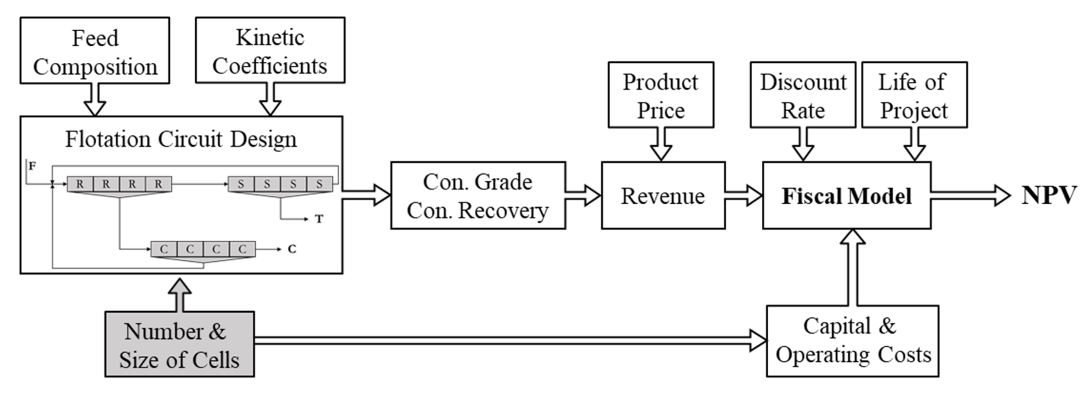
Figure 1 illustrates different components of the mathematical formulation showing the “Number and Size of Cells” as a critical component in determining both technical measures (e.g., concentrate grade and recovery) and financial measures (e.g., capital and operating costs). Table 1 lists the symbols used to describe the problem and categorizes them into sets and indices, variables, certain constants, and potentially uncertain constants. The balance of this section describes the distinct parts of the circuit design deterministic strategy.

2.1. Objective Function

Flotation circuit design optimization problems may be built upon technical (e.g., recovery or grade maximization) and financial (e.g., revenue maximization or cost minimization) objective functions. However, the importance of total life cycle cost analysis necessitates NPV as the objective of the optimization problem. NPV accurately considers the lifetime operation and maintenance costs as well as the initial investments. Therefore, the deterministic formulation seeks to identify the optimal number (N) and size (V) of cells for each flotation stage to maximize the NPV of the project. The NPV of separation circuit design (i.e., objective function) may be adequately expressed in terms of revenue (Rev), operating cost (Opex), capital cost (Capex), discount rate (DRate), and life of the project (Life), as follows:
M a x .   R e v O p e x × 1 1 + D R a t e L i f e D R a t e C a p e x
where the discount rate and the life of project are explicitly specified; while other financial variables in the objective function (i.e., Rev, Opex, Capex) must be accurately determined. The maximization of the proposed objective function is achieved through the maximization of revenue and minimization of associated capital and operating costs. The following subsections describe the calculation of these flotation economic parameters along with flotation metallurgical factors.

2.2. Modeling of Flotation Economics

As shown in Figure 1, the annual revenue of a flotation plant can be derived as the function of both technical parameters (e.g., yield and concentrate grade) as well as financial factors (e.g., price and downstream costs) [17]. For the base metal flotation plants, the following expression may be used to estimate the gained revenue from concentrate sales:
R e v = T F × Y C × F P × G C u × q R f c Y C × T r c
where T F and Y C are the hourly flow rate of the plant feed and concentrate stream, G C is the final concentrate grade, and q is the metal quotation on the commodities market. Furthermore, downstream smelters apply further charges, including refinery cost ( R f c ), treatment cost ( T r c ), grade deduction ( u ), and fraction of metal paid ( F P ), to produce a saleable metal. Treatment charges are imposed based on the concentrate tonnage ( Y C ) while the refinery charges are defined according to a metal content ( G C ). On the other hand, the grade deduction and the fraction of metal paid depend on the recovery efficiency of the smelter. While not visible in Equation (2), the expected annual revenue of the plant depends on the size and number of flotation cells as operational factors (e.g., Y C ,   G C ) are indirectly estimated in terms of cell size and number.
For a flotation plant, the direct operating cost is the sum of power, direct labor, reagents, and maintenance. While these individual values can vary considerably between different operations, one approach to model the cost for analytical purposes is to make a simplifying assumption that ratio of power cost to total operating cost (PcR) remains fixed despite changes to cell size [14]. Thus, if the flotation cell power intensity (OpH, kW/m3) remains fixed, the total operating cost will scale linearly with respect to cell size, as given by:
O p e x = i N i × 24 × E n e r g y × D a y s × O p H P c R × V i 1 h
where N i and V i are the number and size of cells in the ith flotation stage, E n e r g y is the energy cost, D a y s are the number of working days per year, and h is a constant. Data from the literature suggest that the power to total cost ratio (PcR) can vary from 40% to as high as 70% with the lower values representing larger modern flotation cells with optimized power input [14,28]. For the purpose of this analysis, a PcR value of 0.4 was selected along with a power intensity (OpH) of 2.4 Kw/m3. In cases where operational data are available Equation (3) may be substituted for a more sophisticated model.
Flotation plant capital costs can be estimated using a standard exponential scaling law as given by [14,17]:
C a p e x = i N i × C a p A × V i C a p B
where C a p A and C a p B are both constants. For this analysis, C a p B was assumed to be 0.57 coinciding with the economic model given by [14]. Together, Equations (3) and (4) indicate how plant operating and capital costs increase with increasing cell size and number.

2.3. Modeling of Flotation Metallurgy

The separation performance of the flotation system directly defines the annual revenue as circuit yield ( Y C ) and concentrate grade (GC) are the only two variables in the general revenue formulation (see Equation (2)). In other words, the maximization of revenue is possible via an optimal circuit separation performance with high values of yield and concentrate grade. The circuit yield, or mass recovery, and concentrate grade are both can be determined in terms of mass flow rate of mineral species within feed and concentrate streams, as follows:
Y C = T C T F × 100
G C = T O , C T O , F × r m e t m i n × 100
where TC and TF are the total solid flow rates in the concentrate and feed streams, TO,C and TO,F are the ore mass flow rate in the concentrate and feed streams, and r m e t m i n is the mass ratio of the pure metal in the mineral. For example, this ratio for copper associated with chalcopyrite mineral is equal to 0.346. As shown in Equation (6), the accurate estimation of circuit performance indicators requires the precise determination of the mass flow rate of various mineral species within circuit streams.
According to Noble and Luttrell [29], the “matrix reduction algorithm”, as an efficient and accurate tool, can be utilized to estimate the mass flow rate of mineral species within the separation circuit streams. The algorithm relies on three circuit-descriptive matrices (i.e., the feed and product matrices as well as the initial condition vector) and a single governing equation to solve the final circuit stream solution. Table 2 shows the dimension and elements of these matrices. As a note, in the matrix reduction algorithm, junction units are considered as individual stages.
The FMatrix specifies whether jth stream provides feed for the ith stage or not. The value of Fj,i is 1 if stage i is fed by stream j while the zero value of Fj,i indicates that stream j does not feed unit i. Similarly, in constructing PMatrix, the relationship between stream j and unit i is investigated. Elements of this matrix may vary between 0, indicating no relation between stream j and stage i, and 1, specifying that the entire product of the stage i (junction unit) reports into stream j. The values of PMatrix elements determine the probability that the distinct class of species, which feed into unit i, report to stream j. It is worth noting that each specific class of particles (e.g., ore or gangue) requires a unique product matrix (PMatrix) using the numerical values of unit recovery for that particle class. Furthermore, the initial condition vector (CVector) demonstrates the original circuit feed stream(s) and initializes the mass flow rate of different mineral species in the feed stream. As such, a distinct mineral has a unique CVector. If stream j is a circuit feed stream, the value of the feed mass flow rate is assigned to the grade (mass) of mineral in the feed stream (GF). All other elements are assigned a value of zero.
After construction of these fundamental matrices, Equations (7) and (8) may be used to estimate the mass flow rate of each mineral species in all separation circuit streams (TS,j), thereby calculating the total mass flow rate in each stream (Tj):
T S , j = I j , i P M a t r i x , S × F M a t r i x , S 1 × C V e c t o r
T j = S T S , j
In the current optimization formulation, the recovery of individual mineral species within each flotation stage is considered variable to be determined. As a result, the following equation, based on the first-order rate equation for a series of perfectly-mixed cells, may be employed to adequately determine the recovery of each particle class in the ith stage (PS,i):
P S , i = 1 1 K S , i τ i 1 + K S , i τ i N
where KS,i is the kinetic coefficient constant for the particle class of S in the ith unit, and τi is the retention time in each flotation bank of N cells. KS,i is typically estimated using a systematic lock-cycle and pilot scale experimentation. One of the most important parameters in sizing a flotation cell and improving the circuit performance is retention time. The mean retention time can be expressed as the ratio of active cell volume to the cell volumetric flow rate utilizing the following formulation:
τ i = 60 × V i T i S G + T i X i T i
where Ti is the feed mass of ith individual stage, SG is the solid density, and Xi is the solid concentration in 
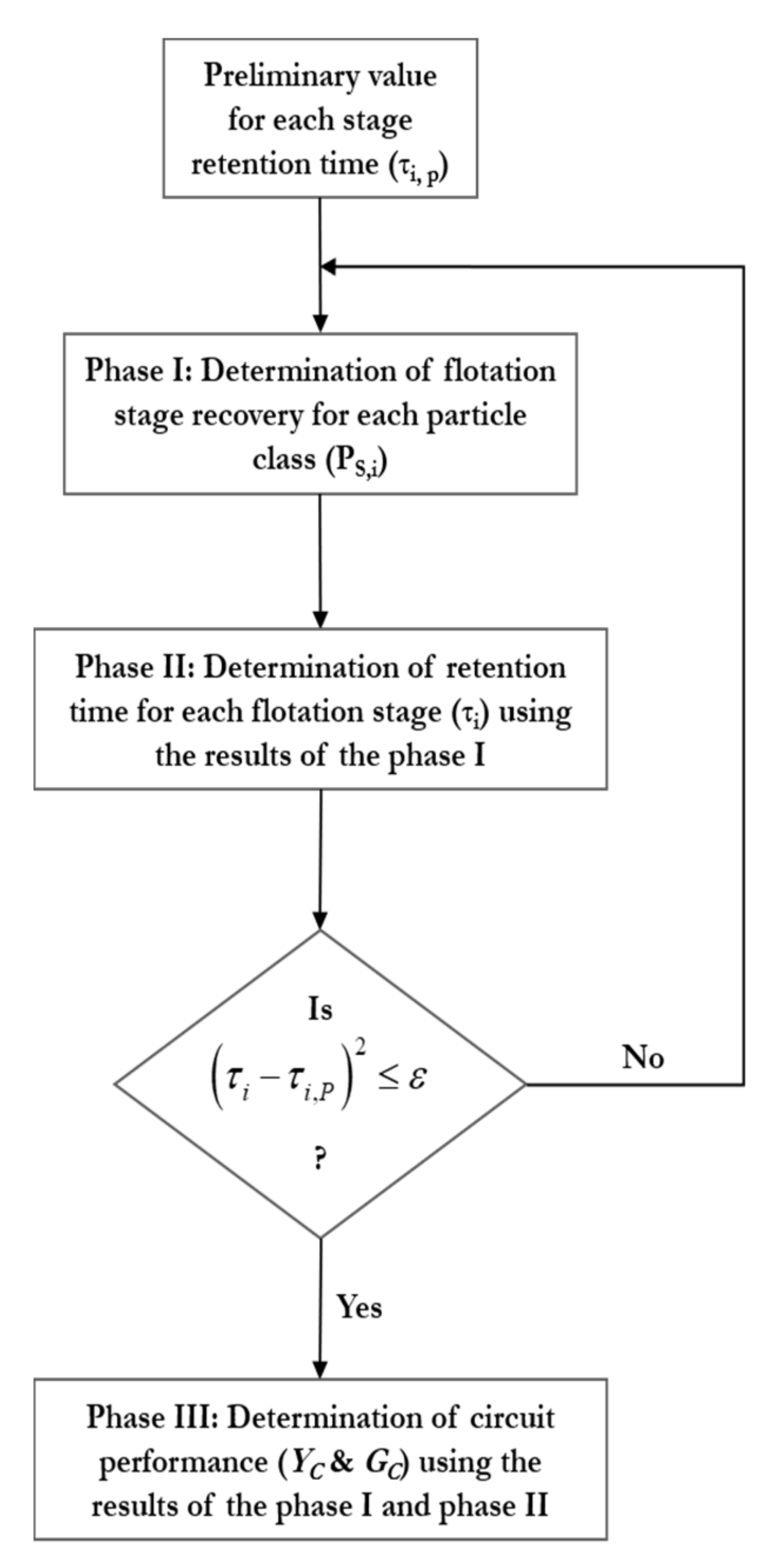
ith stage. As illustrated in Equations (9) and (10), the unit recovery and retention time factors are dependent. In other words, to accurately identify the optimal values of retention time in individual flotation stages, the proper values of recoveries are required, and vice versa. These values are typically solved via iterative calculations. To appropriately estimate these variables, an innovative approach is implemented in which the optimization problem is initiated employing a set of preliminary retention time values (τi,P) in each flotation bank. These values are then applied in Equation (9) to calculate the unit recovery values. In the next phase, the calculated recovery values are employed to determine the secondary values for the retention times associated with each flotation bank. The calculated values of retention time then replace the preliminary retention time values and this procedure is repeated until the following constraint is satisfied. It is worth noting that the following constraint is evaluated concurrently with the optimization problem:
τ i τ i , P 2 ε
where ε may be considered as a very small number. Following the results of these phases, the circuit mass yield and the final concentrate grade are determined. Figure 2 depicts the described procedure for the accurate estimation of technical parameters in terms of number and size of flotation cells.

2.4. Arbitrary Constraints

Overall, the proposed techno-economic formulation for determining the optimum number and size of cell in the flotation system is placed into the category of non-convex mixed integer non-linear program class (MINLP). Typically, various methodologies and optimization solvers may be utilized to properly solve these types of mathematical models. However, given the high complexity of this optimization model, the majority of available techniques are computationally expensive. As such, the following constraints are suggested to be added into the original strategy for the effective reduction in the size of the model.
Constraints on the size (V) and number (N) of flotation cells. These constraints can be added to the general formulation according to the available cell sizes in the industry and typical number of cells in an individual flotation bank. Based on these observations, the following constraints are imposed:
N m i n N i N m a x
V m i n V i V m a x
Constraints on the concentrate grade (GC). This constraint is mainly dictated by downstream smelters considering the technological limitation of the smelting process. The following concentrate grade constraint indirectly limits the mass yield projected by the flotation system:
G C , m i n G C
Based on the complexity of the given flotation circuit configuration, several constraints on the stage recovery and retention time values may be added to the original formulation.

2.5. Model Implementation and Limitations

All the mathematical models in this study were coded in the GAMS platform (GAMS Development Corporation, Fairfax, VA, USA) and solved by BARON [30] on a Dell Studio PC with Intel(R) Xeon(R) CPU E5-1607 processor running at 3.00 GHz and 16.0 GB of RAM under a 64-bit Windows operating system. The computational time is largely dependent on the number of iterations, the circuit complexity, and the use of a local versus a global optimization solver. Moreover, flotation circuit optimization is often constrained by site-specific conditions and non-technical factors. The approach employed in this study does introduce some simplifying assumptions to improve computational requirements; however, these inputs can be expounded if realistic site data are available.
It should also be noted that the current approach specifically addresses the optimization of the size and volume of flotation cells with an assumed circuit structure. Thus, in a more open-ended design problem, the methodology would best be used to augment an existing technique to evaluate circuit structures such as that proposed by Noble and Luttrell [26].

3. Stochastic Optimization of Circuit Design

3.1. Sensitivity Analysis of Uncertain Parameters

As described in the introduction section, the techno-economic parameters involved in the separation circuit design and operation may be subject to different degrees of uncertainties. The current study considers metal price, feed grade, and kinetic coefficient as the potentially uncertain variables (Table 1). While the commodity market completely controls the uncertainty associated with the metal price, the heterogeneity of run-of-mine materials, the variability in operational parameters, and experimental and measurement errors may generate various uncertainty levels in the feed grade and kinetic coefficient factors.
The addition of input parameter uncertainty grossly elevates the complexity of the proposed MINLP model, and this complexity is further elevated with each additional uncertain input factor. As a result, the number of uncertain factors should be minimized by a rigorous preliminary assessment of the model sensitivity. The optimal circuit solution is separately identified at three levels of each uncertain parameter and then the significance of each parameter’s uncertainty is investigated. The importance of each factor in identifying the final circuit solution indicate whether the parameter must be considered uncertain in the final stochastic formulation.

3.2. Sample Average Approximation Approach

The sample average approximation (SAA) methodology is a common technique for solving large-scale optimization problems by the means of Monte Carlo simulation (MCS). In this technique, a set of random numbers, representing the uncertain parameter, is generated and then the expected value of objective function is determined utilizing a sample average approximation derived from these random numbers. The ultimate stochastic problem is then solved using a deterministic optimization technique. The process is replicated several times employing different sets of random numbers, and finally, the optimal candidate solutions are gathered and compared against one another. Several authors have extensively reviewed the principles of the SAA method along with its implementation in different areas of stochastic optimization [31,32,33]. For the simple illustration of the SAA approach, the following optimization problem formulation is considered:
m i n x S g x : = Ε P G x , W
where W (uncertain constant) is a set of random numbers with a probability distribution of P, S is a finite number of set, G(x,W) is a real valued function in terms of x and W, and EP G(x,W) is the corresponding expected value.
Now, let W 1 ,   ,   W N be an independently and identically distributed random sample of N realizations of the random vector W. The SAA form of the original formulation can be expressed as:
m i n x S g ^ N x : = 1 N j = 1 N G x , W j
The SAA stochastic problem is then solved repeatedly using a deterministic optimization algorithm. By generating S independent random number samples, with the size of N, and solving the associated SAA problems, the final objective function values of g ^ N 1 x 1 ,   g ^ N 2 x 2 ,     ,   g ^ N R x R and candidate solutions of x 1 , x 2 ,   , x R   are obtained. Of all alternative optimal solutions, typically, the one that generates the minimum value of objective function and those with highest frequency may be selected as the final optimal solutions of the stochastic problem.
The current study addresses the capability of SAA methodology for finding the optimal size and number of cells in the flotation system under uncertainty. According to the sensitivity analysis results, significant uncertain parameters are incorporated in the original MINLP problem as a set of random numbers with the defined probability distributions (e.g., uniform, normal, and lognormal) having the similar statistical measures. As such, the proposed strategy investigates the impact of distribution functions, that represent uncertain parameters, on the final circuit solution. The constructed stochastic optimization problem is then solved repeatedly for different sets of random numbers estimating the NPV values. The final solution for the stochastic problem is the one with the maximum NPV value and the most repeated solutions (i.e., the most robust solution). Finally, the obtained results from this phase of the study are compared against the deterministic problem circuit solution. This comparison indicates the importance of considering uncertainty in the process of finding the optimal flotation system and shows the significance of statistical distribution types for various uncertain parameters.

4. Application Example

4.1. Problem Description

To properly demonstrate the implementation of the proposed techno-economic optimization strategy, a simple cell-based flotation circuit configuration is provided (Figure 3). This balanced flotation circuit with recycling concentrate and tailings streams to the rougher stage and is designed to treat a chalcopyrite mineral. It is assumed that this flotation circuit represents one of the several alternative circuits that are selected through pareto-based circuit design process. The main goal is to determine the most profitable flotation circuit design candidates with the proper size and number of cells. The alternative circuit solutions may then be selected for further laboratory and pilot-scale experimentations.
Table 3 shows the values of different input parameters, including certain and potentially uncertain constants. The flotation circuit treats 1000 tons per hour of ore containing 0.1% of chalcopyrite (10 tons per hour) on average. The downstream smelter is specified the minimum concentrate grade of 25%. The maximum and minimum available flotation cell sizes are considered to be 250 and 10 cubic meters. It is worthwhile to note that the numerical input parameters (e.g., available volumes for cells and feed grade) are selected to demonstrate the applicability of the developed optimization routine and may be altered for different applications.

4.2. Deterministic Results

Table 4 reports results of the deterministic problem when all financial and technical factors (i.e., price, feed grade, and kinetic coefficients) are considered as static values. The data indicate that the three-stage flotation circuit is capable of producing a final concentrate with 25% chalcopyrite at 97.34% global recovery value. The implementation of larger size cells in the rougher and scavenger stages and two 16 m3 flotation cells in the cleaner stage leads to a total 25-year NPV of USD16.7 million.

4.3. Sensitivity Analysis

4.3.1. Copper Price

The original deterministic problem is separately solved at three levels of copper price (i.e., 4000, 6000, and 8000 USD/ton) while other potentially uncertain constants (i.e., feed grade and kinetic coefficients) remain at their initial static values. Given the optimal size and number of flotation cells in each case, the associated financial and technical parameters to each design are then determined at all three levels of copper price. As such, for each copper price case, three different flotation circuit designs are examined and compared against one another. Table 5 summarizes results of the sensitivity analysis study on the copper price.
As expected, the metal price element has a significant impact on the projected financial indicators. For instance, an increase in the copper price from USD6000 to USD8000 per ton will improve the NPV by approximately 50%. As shown in Table 5, the operating and capital cost of the flotation circuit remains unchanged unless the number and size of flotation cells are varied. These data indicate that different combinations of cell size and number may produce a similar NPV. In other words, price uncertainty may not necessarily affect the optimal design parameters as the optimal cell number and size at a specific price case will remain as one of the optimal solutions for other scenarios. This statement is valid when the flotation circuit structure is fixed, and the plant is constrained to meet a specific concentrate grade requirement.
This observation can be considered as a supplement to the results of Cisternas et al. on the significant impact of metal price on the optimal circuit structure [34,35]. Despite the executed approach, they examined the importance of metal price, as a stochastic uncertainty source, on the optimal circuit structure. Therefore, it can be concluded that the uncertainty of metal price is a significant factor in the optimal design of circuit structure and insignificant in the selection of the equipment sizing parameter when circuit structure is known and concentrate grade constraint is considered.

4.3.2. Feed Composition

In the next phase of the study, the sensitivity of circuit solutions to the level of chalcopyrite concentration in the feed stream was evaluated. The level of metal grade in the plant feed can strongly affect the circuit separation performance as it may vary the associated kinetic coefficients. Despite this fact, in addition to the copper price, ore and gangue kinetic coefficients are kept constant in all three flotation banks. Like the prior phase of the study, the optimal circuit solution is determined for individual feed grade condition and then, the optimality of those data at other degrees of feed grade is investigated.
As indicated in Table 6, even the slightest variation in the feed composition, a 0.5% increase, can substantially alter the value of circuit techno-economic measures. Solving the deterministic MINLP problem at distinct levels of feed grade results in obtaining a unique equipment sizing solution for each case. Nevertheless, the optimal solution for one case has the capability to produce the maximum NPV at various degrees of feed grade, albeit at different levels of concentrate grade and yield. For example, the evaluation of the optimal circuit solution for the high-grade case (i.e., 5, 1, and 1 flotation cell with the volume of 205, 190, and 50 cubic meters) at lower levels of feed grade shows that the maximum NPV is achievable at lower values of concentrate grade and yield. These observations indicate the importance of feed grade uncertainty in the optimal selection of equipment sizing when limitation on the final concentrate grade is specified. As such, unlike metal price, the uncertainty of feed grade parameters is considered in the stochastic circuit optimization problem.
Previous studies by Cisternas et al. [34,35] demonstrated the importance of feed grade variation, as a stochastic uncertainty source, in the optimal design of flotation circuit structure. The results of the current study show that feed grade is not an influential factor in the optimal selection of flotation equipment sizing when the structure is fixed, and no concentrate grade constraint is considered (Table 6). However, in the presence of concentrate grade constraint, uncertainty of feed grade must be considered in the optimal design of flotation size and volume in each cleaning stage.

4.3.3. Kinetic Coefficients

The kinetic coefficient values in Table 4 are varied by ± 20 % and the deterministic circuit optimization problem is solved at the designated three levels of the kinetic coefficients for ore and gangue in all three flotation banks. Overall, the sensitivity analysis study on kinetic coefficients shows a slight increase in the NPV at higher kinetic coefficient values (Table 7). The optimal circuit solutions demonstrate the need for larger size cells at lower kinetic levels for producing the concentrate of 25% grade. The rise in the kinetic constants in these large flotation cells results in the lower concentrate grade and higher yield values. Altogether, these data indicate the significant impact of the kinetic coefficient factor on the optimal circuit solution. As a result, the stochastic optimization routine must address the variability of this factor, besides feed grade, in the optimal design formulation. This conclusion is verified by previous studies on the importance of kinetic coefficient variability, as a source of epistemic uncertainty, on the optimal sizing of flotation equipment [25].

4.4. Stochastic Circuit Design Optimization

Following the sensitivity analysis, the SAA method aims to find the optimal number and size of flotation cells for the three-stage flotation system. The resultant stochastic approach considers the feed grade and kinetic coefficients as uncertain parameters while the metal price value is kept at USD 6000. As a result, the chalcopyrite flow rate in the feed stream (i.e., feed grade) and the kinetic coefficient parameters are incorporated in the original model with uniform, normal, and lognormal probability distribution functions. According to Helton and Oberkampf [36], epistemic uncertainty sources must be incorporated in the mathematical models using uniform distribution functions. On the other hand, variables with stochastic uncertainty are suggested to be considered in the models using normal distribution functions. Despite these recommendations, the goal of the current study is to further investigate the impact of distribution function types on the final circuit solution.
For each case, 10,000 random numbers are generated, the simulation is repeated 20 times, and then alternative optimal solutions are identified. For each statistical distribution, two circuit solutions are selected according to their profitability and frequency among all 20 results. Finally, these six stochastic circuit solutions are compared against the optimal design obtained from the deterministic formulation. Table 8 shows the statistical measures of uncertain input parameters used in the stochastic optimization procedure.
Figure 4 depicts the value of objective functions (NPV) for all three cases of statistical distributions throughout the 20 scenarios of stochastic optimization. Of all scenarios, one solution with the highest level of NPV (green marker) and one with the highest frequency (red marker) are selected as the alternative optimal circuit solutions. Additionally, Figure 5 indicates the results of the SAA approach alongside the deterministic circuit solution.
The comparison between stochastic and deterministic circuit design solutions (Figure 5) demonstrates the significance of considering uncertainty in the flotation circuit design procedure. The input parameters’ statistical distribution can play a significant role, as each distribution type may produce a different circuit solution. Interestingly, the results of all 20 scenarios in the SAA approach, regardless of distribution shape, select a cleaner bank containing only one flotation cell with the size of between 36 to 40 m3. More interestingly, according to the 20 scenario observations, the highest frequency solution (and possibly the most robust solution) is identical in all statistical distribution cases.
Finally, the optimality of stochastic circuit solutions in the original deterministic model is investigated. This analysis indicates that none of the stochastic circuit solutions are placed in the category of optimal solutions for the deterministic problem. These observations verify the essential need for considering uncertainty in the process of flotation circuit design.

5. Conclusions

The optimal selection of the size and number of cells in the cell-based flotation circuit design is a vital part of an effective flotation design procedure as these factors directly define the circuit financial measures. Additionally, a comprehensive circuit optimization strategy must address the uncertainty associated with various techno-economic parameters, including price, feed grade, and kinetic coefficients. In this study, an innovative stochastic optimization approach was developed for finding the optimal flotation equipment design parameters with the objective of maximizing NPV. After completion of a systematic sensitivity analysis, feed grade and kinetic coefficient were incorporated in the optimization model based on various statistical distributions. The Sample Average Approximation approach as a Monte Carlo-based technique was employed to select alternative optimal flotation circuit solutions. The following conclusions are drawn:
  • Results of the proposed circuit optimization strategy indicate that multiple circuit solutions (number and size of flotation cells) may produce a maximum NPV;
  • Despite the importance of the metal price in determining the circuit profitability and circuit structure, its associated variability does not necessarily affect the optimal circuit design solution when the circuit structure is fixed and a concentrate grade constraint is applied;
  • Alternatively, uncertainties in the kinetic coefficient have a significant role in defining the metallurgical performance of the flotation circuit, thereby affecting both circuit profitability and circuit design solution;
  • The circuit solutions of the SAA approach do not necessarily produce the maximum NPV when compared with the deterministic case. In other words, the solutions of stochastic problem may not appear as a deterministic solution. This observation demonstrates the importance of considering uncertainty in the flotation circuit design procedure;
  • Uncertain parameters were incorporated into the circuit design problem following different probability distribution functions. However, regardless of the distribution types, the SAA approach introduces an identical circuit solution as a design with highest frequency (i.e., the most robust solution).

Author Contributions

Conceptualization, methodology, formal analysis, and investigation, S.H.A. and A.N.; writing—original draft preparation, S.H.A.; writing—review and editing, supervision, project administration, A.N. All authors have read and agreed to the published version of the manuscript.

Funding

The authors would like to acknowledge the financial contribution from Virginia Tech’s Open Access Subvention Fund, which helped to cover the open access article process charges.

Conflicts of Interest

The authors declare no conflict of interest.

References

  1. Fuerstenau, M.C.; Han, K.N. Principles of Mineral Processing; The Society for Mining, Metallurgy, and Exploration, Inc.: Littleton, CO, USA, 2003; 573p. [Google Scholar]
  2. Fuerstenau, M.C.; Jameson, G.; Yoon, R. Froth Flotation: A Century of Innovation; The Society for Mining, Metallurgy, and Exploration, Inc.: Littleton, CO, USA, 2007; 891p. [Google Scholar]
  3. Wills, B.A.; Finch, J. Wills’ Mineral Processing Technology: An Introduction to the Practical Aspects of Ore Treatment and Mineral Recovery, 8th ed.; Butterworth-Heinemann: Oxford, UK, 2015; 512p. [Google Scholar]
  4. Amini, S.H.; Noble, A. Predicting and interpreting uncertainty propagation in separation circuits using functional unit evaluation. Miner. Eng. 2019, 142, 105886. [Google Scholar] [CrossRef]
  5. Amini, S.H.; Noble, A. Application of linear circuit analysis in the evaluation of mineral processing circuit design under uncertainty. Miner. Eng. 2017, 102, 18–29. [Google Scholar] [CrossRef]
  6. Yingling, J.C. Parameter and configuration optimization of flotation circuits, part II. A new approach. Int. J. Miner. Process. 1993, 38, 41–66. [Google Scholar] [CrossRef]
  7. Mandani, F.; Camarda, K. Multi-objective Optimization for Plant Design via Tabu Search. In Proceedings of the 28th European Symposium on Computer Aided Process Engineering, Graz, Austria, 13 June 2018; Volume 43, pp. 543–548. [Google Scholar] [CrossRef]
  8. Green, J. The optimisation of flotation networks. Int. J. Miner. Process. 1984, 13, 83–103. [Google Scholar] [CrossRef]
  9. Reuter, M.A.; van Deventer, J.S.J.; Green, J.C.A.; Sinclair, M. Optimal design of mineral separation circuits by use of linear pro-gramming. Chem. Eng. Sci. 1988, 43, 1039–1049. [Google Scholar] [CrossRef]
  10. Reuter, M.; Van Deventer, J. The use of linear programming in the optimal design of flotation circuits incorporating regrind mills. Int. J. Miner. Process. 1990, 28, 15–43. [Google Scholar] [CrossRef]
  11. Guria, C.; Verma, M.; Gupta, S.K.; Mehrotra, S.P. Simultaneous optimization of the performance of flotation circuits and their sim-plification using the jumping gene adaptations of genetic algorithm. Int. J. Miner. Process. 2005, 77, 165–185. [Google Scholar] [CrossRef]
  12. Guria, C.; Verma, M.; Mehrotra, S.P.; Gupta, S.K. Multi-objective Optimal Synthesis and Design of Froth Flotation Circuits for Mineral Processing, Using the Jumping Gene Adaptation of Genetic Algorithm. Ind. Eng. Chem. Res. 2005, 44, 2621–2633. [Google Scholar] [CrossRef]
  13. Guria, C.; Varma, M.; Mehrotra, S.P.; Gupta, S.K. Simultaneous optimization of the performance of flotation circuits and their simplification using the jumping gene adaptations of genetic algorithm-II: More complex problems. Int. J. Miner. Process. 2006, 79, 149–166. [Google Scholar] [CrossRef]
  14. Abu-Ali, M.; Sabour, S.A. Optimizing the design of flotation circuits: An economic approach. Miner. Eng. 2003, 16, 55–58. [Google Scholar] [CrossRef]
  15. Cisternas, L.A.; Gálvez, E.D.; Zavala, M.F.; Magna, J. A MILP model for the design of mineral flotation circuits. Int. J. Miner. Process. 2004, 74, 121–131. [Google Scholar] [CrossRef]
  16. Cisternas, L.A.; Méndez, D.A.; Gálvez, E.D.; Jorquera, R.E. A MILP model for design of flotation circuits with bank/column and regrind/no regrind selection. Int. J. Miner. Process. 2006, 79, 253–263. [Google Scholar] [CrossRef]
  17. Schena, G.; Villeneuve, J.; Noël, Y. A method for a financially efficient design of cell-based flotation circuits. Int. J. Miner. Process. 1996, 46, 1–20. [Google Scholar] [CrossRef]
  18. Schena, G.; Zanin, M.; Chiarandini, A. Procedures for the automatic design of flotation networks. Int. J. Miner. Process. 1997, 52, 137–160. [Google Scholar] [CrossRef]
  19. Lucay, F.A.; Gálvez, E.D.; Cisternas, L.A. Design of Flotation Circuits Using Tabu-Search Algorithms: Multispecies, Equipment Design, and Profitability Parameters. Minerals 2019, 9, 181. [Google Scholar] [CrossRef] [Green Version]
  20. Cisternas, L.A.; Lucay, F.; Gálvez, E.D. Effect of the objective function in the design of concentration plants. Miner. Eng. 2014, 63, 16–24. [Google Scholar] [CrossRef]
  21. Cisternas, L.A.; Gálvez, E.D.; Mendez, D.A. Optimal Design of Flotation Circuits Including Selection of Bank Cells, Column Cells, and Regrinding Mills. In Proceedings of the 4th Mercosur Congress on Process Systems Engineering: 2nd Mercosur Congress on Chemical Engineering, Rio de Janeiro, Brazil, 14–18 August 2005; pp. 1–10. [Google Scholar]
  22. Ghobadi, P.; Yahyaei, M.; Banisi, S. Optimization of the performance of flotation circuits using a genetic algorithm oriented by process-based rules. Int. J. Miner. Process. 2011, 98, 174–181. [Google Scholar] [CrossRef]
  23. Cisternas, L.A.; Lucay, F.A.; Acosta-Flores, R.; Gálvez, E.D. A quasi-review of conceptual flotation design methods based on computational optimization. Miner. Eng. 2018, 117, 24–33. [Google Scholar] [CrossRef]
  24. Jamett, N.; Cisternas, L.A.; Vielma, J.P. Solution strategies to the stochastic design of mineral flotation plants. Chem. Eng. Sci. 2015, 134, 850–860. [Google Scholar] [CrossRef] [Green Version]
  25. Acosta-Flores, R.; Lucay, F.; Cisternas, L.; Gálvez, E. Two-phase optimization methodology for the design of mineral flotation plants, including multispecies and bank or cell models. Miner. Met. Process. 2018, 35, 24–34. [Google Scholar] [CrossRef]
  26. Noble, A.; Luttrell, G.H. Value-based objective functions applied to circuit analysis. Min. Met. Explor. 2015, 32, 45–58. [Google Scholar] [CrossRef]
  27. Pirouzan, D.; Yahyaei, M.; Banisi, S. Pareto based optimization of flotation cells configuration using an oriented genetic algorithm. Int. J. Miner. Process. 2014, 126, 107–116. [Google Scholar] [CrossRef]
  28. Rinne, A.; Peltola, A. On lifetime costs of flotation operations. Miner. Eng. 2008, 21, 846–850. [Google Scholar] [CrossRef]
  29. Noble, A.; Luttrell, G.H. The matrix reduction algorithm for solving separation circuits. Miner. Eng. 2014, 64, 97–108. [Google Scholar] [CrossRef]
  30. Tawarmalani, M.; Sahinidis, N.V. A polyhedral branch-and-cut approach to global optimization. Math. Program. 2005, 103, 225–249. [Google Scholar] [CrossRef]
  31. Bardossy, M.G.; Raghavan, S. An inexact sample average approximation approach for the stochastic connected facility location problem. Networks 2017, 70, 19–33. [Google Scholar] [CrossRef]
  32. Verweij, B.; Ahmed, S.; Kleywegt, A.J.; Nemhauser, G.; Shapiro, A. The Sample Average Approximation Method Applied to Stochastic Routing Problems: A Computational Study. Comput. Optim. Appl. 2003, 24, 289–333. [Google Scholar] [CrossRef]
  33. Mak, W.-K.; Morton, D.P.; Wood, R. Monte Carlo bounding techniques for determining solution quality in stochastic programs. Oper. Res. Lett. 1999, 24, 47–56. [Google Scholar] [CrossRef]
  34. Cisternas, L.A.; Jamett, N.; Gálvez, E.D. Approximate recovery values for each stage are sufficient to select the concentration circuit structures. Miner. Eng. 2015, 83, 175–184. [Google Scholar] [CrossRef]
  35. Acosta-Flores, R.; Lucay, F.A.; Gálvez, E.D.; Cisternas, L.A. The effect of regrinding on the design of flotation circuits. Miner. Eng. 2020, 156, 106524. [Google Scholar] [CrossRef]
  36. Helton, J.; Oberkampf, W. Alternative representations of epistemic uncertainty. Reliab. Eng. Syst. Saf. 2004, 85, 1–10. [Google Scholar] [CrossRef]
Figure 1. Cell-based flotation circuit design problem.
Minerals 11 00459 g001
Figure 2. Symbolic diagram of the decision procedure for the determination of the flotation performance indicators (e.g., yield and concentrate grade).
Minerals 11 00459 g002
Figure 3. A balanced circuit used for the application example.
Minerals 11 00459 g003
Figure 4. The value of objective function for different scenarios of the stochastic optimization solutions.
Minerals 11 00459 g004
Figure 5. Comparison between the optimal results of the deterministic and stochastic methodologies.
Minerals 11 00459 g005
Table 1. Description of symbols used for sets, indices, variables, certain constants, and potentially uncertain constants.
Nomenclature
Sets & indicesCertain constants
inumber of flotation stagesDRatediscount rate
jnumber of circuit streamsLifelife of the project
VariablesFPfraction of metal paid
Revrevenueugrade deductions
Opexoperating costRfcrefinery charges
Capexcapital costTrctreatment charges
YCmass yield to concentrate streamTFfeed mass flow rate
GCgrade of valuable mineral in concentrate streamTO,Fore mass flow rate in feed stream
Ninumber of cells in ith flotation stageEnergyenergy cost
Visize of cells in ith flotation stageDaysnumber of working days per year
TCsolid flow rate in the concentrate streamOpHpower cost factor kWh per m3 of the cell size
TO,Core flow rate in the concentrate streamhconstant
TS,jmass flow rate of mineral S in jth streamCapAconstant
Tjtotal mass flow rate in jth stream CapBconstant
PS,irecovery of mineral S in the ith stage rmet/minmass ratio of the pure metal in the mineral
τiretention time in ith flotation bank SGsolid density
Tifeed mass of ith flotation stagePcRratio of power cost to total operating cost
τi,Ppreliminary retention time in ith flotation bankXisolid concentration in ith flotation stage
Potential uncertain constants
qmetal price
KS,ikinetic coefficient for mineral S in the ith unit
GFfeed grade
Table 2. Circuit-descriptive matrices utilized in the matric reduction algorithm (after [28]).
FMatrixPMatrixCVector
Stage1Stage2StageiStage1Stage2StageiFeed
Stream1F1,1F1,2F1,iP1,1P1,2P1,iC1,1
Stream2F2,1F2,2F2,iP2,1P2,2P2,iC2,1
StreamjFj,1Fj,2Fj,iPj,1Pj,2Pj,iCj,1
Table 3. Input parameters in the deterministic circuit optimization problem.
Potential Uncertain ConstantsCertain Constants
q (USD/ton)6000Drate (%)10
GF (%) 0.01Life (year)25
KO,R (L/min)0.225FP0.975
KO,S (L/min)0.2U0.01
KO,C (L/min)0.275Rfc (USD/ton)200
KG,R (L/min)0.005Trc (USD/ton)55
KG,S (L/min)0.01TF (ton/h)1000
KG,C (L/min)0.0075TO,F (ton/h)10
Energy (USD/kWh)0.07
Days (day/year)340
OpH (kWh/m3 of cell)2.4
H0.04
CapA15,422.88
CapB0.57
rmet/min0.346
SG2.65
XR (%)35.04
XS (%)37.04
XC (%)25.34
Table 4. Optimal flotation circuit solution using the deterministic approach.
Objective FunctionNPV (USD)USD 16.7 Million
Circuit SolutionNR, VR (m3)4, 194
NS, VS (m3) 2, 182
NC, VC (m3)2, 16
Financial Outcomes (Intermediate Calculations)Rev (USD)USD 190 million
Capex (USD)USD 1.99 million
Opex (USD)USD 3.26 million
Technical Outcomes (Intermediate Calculations)PO,R, PG,R (%)93.49, 8.26
PO,S, PG,S (%)74.20, 9.03
PO,C, PG,C (%)65.67, 3.75
Con. grade (%)25.15
Recovery (%)97.34
Table 5. Sensitivity analysis results on the metal price (bold values indicate outcomes at optimal solution).
Price 1: USD4000Price 2: USD6000Price 3: USD8000
Price 1: USD4000Financial outcomesNPV (USD)USD 10.3 millionUSD 16.7 millionUSD 23.3 million
Rev (USD)USD 123 millionUSD 187 millionUSD 252 million
Capex (USD)USD 1.73 millionUSD 1.73 millionUSD 1.73 million
Opex (USD)USD 2.87 millionUSD 2.87 millionUSD 2.87 million
Optimal circuit solutionNR, VR (m3)4, 1974, 1974, 197
NS, VS (m3) 1, 2131, 2131, 213
NC, VC (m3)2, 162, 162, 16
Technical outcomesCon. Grade (%)25.0225.0225.02
Yield (%)1.321.321.32
Price 2: USD6000Financial outcomesNPV (USD)USD 10.3 millionUSD 16.7 millionUSD 23.3 million
Rev (USD)USD 125 millionUSD 190 millionUSD 256 million
Capex (USD)USD 1.99 millionUSD 1.99 millionUSD 1.99 million
Opex (USD)USD 3.27 millionUSD 3.27 millionUSD 3.27 million
Optimal circuit solutionNR, VR (m3)4, 1944, 1944, 194
N, VS (m3) 2, 1822, 1822, 182
NC, VC (m3)2, 162, 162, 16
Technical outcomesCon. Grade (%)25.1525.1525.15
Yield (%)1.341.341.34
Price 3: USD8000Financial outcomesNPV (USD)USD 10.3 millionUSD 16.7 millionUSD 23.3 million
Rev (USD)USD 125 millionUSD 191 millionUSD 256 million
Capex (USD)USD 2.04 millionUSD 2.04 millionUSD 2.04 million
Opex (USD)USD 3.52 millionUSD 3.52 millionUSD 3.52 million
Optimal circuit solutionNR, VR (m3)4, 2114, 2114, 211
NS, VS (m3) 2, 1962, 1962, 196
NC, VC (m3)1, 331, 331, 33
Technical outcomesCon. Grade (%)25.0725.0725.07
Yield (%)1.351.351.35
Table 6. Sensitivity analysis results on the feed grade (bold values indicate outcomes at optimal solution).
Feed Grade 1: 0.5%Feed Grade 2: 1.0%Feed Grade 3: 1.5%
Feed Grade 1: 0.5%Financial outcomesNPV (USD)USD 7.17 millionUSD 16.7 millionUSD 25.1 million
Rev (USD)USD 91.3 millionUSD 182 millionUSD 271 million
Capex (USD)USD 1.7 millionUSD 1.7 millionUSD 1.7 million
Opex (USD)USD 2.62 millionUSD 2.62 millionUSD 2.62 million
Optimal circuit solution NR, VR (m3)4, 1304, 1304, 130
NS, VS (m3) 2, 2002, 2002, 200
NC, VC (m3)1, 151, 151, 15
Technical outcomesCon. Grade (%)25.2429.7331.55
Yield (%)0.641.081.51
Feed Grade 2: 1.0%Financial outcomesNPV (USD)USD 7.2 millionUSD 16.7 millionUSD 26.2 million
Rev (USD)USD 95.2 millionUSD 190 millionUSD 285 million
Capex (USD)USD 1.99 millionUSD 1.99 millionUSD 1.99 million
Opex (USD)USD 3.27 millionUSD 3.27 millionUSD 3.27 million
Optimal circuit solution NR, VR (m3)4, 1944, 1944, 194
NS, VS (m3) 2, 1822, 1822, 182
NC, VC (m3)2, 162, 162, 16
Technical outcomesCon. Grade (%)19.1925.1528.04
Yield (%)0.881.341.79
Feed Grade 3: 1.5%Financial outcomesNPV (USD)USD 7.17 millionUSD 16.7 millionUSD 26.3 million
Rev (USD)USD 95.7 millionUSD 191 millionUSD 287 million
Capex (USD)USD 2.05 millionUSD 2.05 millionUSD 2.05 million
Opex (USD)USD 3.51 millionUSD 3.51 millionUSD 3.51 million
Optimal circuit solution NR, VR (m3)5, 2055, 2055, 205
NS, VS (m3) 1, 1901, 1901, 190
NC, VC (m3)1, 501, 501, 50
Technical outcomesCon. Grade (%)15.4321.7925.22
Yield (%)1.11.562
Table 7. Sensitivity analysis results on the kinetic coefficient (bold values indicate outcomes at optimal solutions).
Low KMedium KHigh K
Low KFinancial outcomesNPV (USD)USD 16.2 millionUSD 16.7 millionUSD 17 million
Rev (USD)USD 185 millionUSD 190 millionUSD 192 million
Capex (USD)USD 1.93 millionUSD 1.93 millionUSD 1.93 million
Opex (USD)USD 3.57 millionUSD 3.57 millionUSD 3.57 million
Optimal circuit solution at low KNR, VR (m3)3, 2503, 2503, 250
NS, VS (m3) 2, 2502, 2502, 250
NC, VC (m3)1, 451, 451, 45
Technical outcomesCon. Grade (%)25.0422.8520.93
Yield (%)1.311.471.63
Medium KFinancial outcomesNPV (USD)USD 16.1 millionUSD 16.7 millionUSD 16.7 million
Rev (USD)USD 185 millionUSD 190 millionUSD 193 million
Capex (USD)USD 1.99 millionUSD 1.99 millionUSD 1.99 million
Opex (USD)USD 3.27 millionUSD 3.27 millionUSD 3.27 million
Optimal circuit solution at medium KNR, VR (m3)4, 1944, 1944, 194
NS, VS (m3) 2, 1822, 1822, 182
NC, VC (m3)2, 162, 162, 16
Technical outcomesCon. Grade (%)27.0625.1523.43
Yield (%)1.211.341.46
High KFinancial outcomesNPV (USD)USD 15.5 millionUSD 16.5 millionUSD 16.9 million
Rev (USD)USD 176 millionUSD 186 millionUSD 191 million
Capex (USD)USD 1.88 millionUSD 1.88 millionUSD 1.88 million
Opex (USD)USD 2.58 millionUSD 2.58 millionUSD 2.58 million
Optimal circuit solution at high KNR, VR (m3)4, 1404, 1404, 140
NS, VS (m3) 4, 804, 804, 80
NC, VC (m3)1, 271, 271, 27
Technical outcomesCon. Grade (%)28.1926.5925.04
Yield (%)1.111.241.35
Table 8. Statistical measures of the uncertain input parameters in the stochastic circuit design problem.
Input FactorsMeanStandard Deviation
TO,F (ton/h)103
KO,R (L/min)0.22500.0900
KO,S (L/min)0.20000.0800
KO,C (L/min)0.27500.1100
KG,R (L/min)0.00500.0020
KG,S (L/min)0.01000.0040
KG,C (L/min)0.00750.0030
Publisher’s Note: MDPI stays neutral with regard to jurisdictional claims in published maps and institutional affiliations.

