Assessment of Annual Physico-Chemical Variability via High-Temporal Resolution Monitoring in an Antarctic Shallow Coastal Site (Terra Nova Bay, Ross Sea)

Abstract

The Southern Ocean is an important atmospheric carbon sink, and potential changes in the carbon flux in this region will affect the ocean as a whole. Thus, to monitor the variability of its physico-chemical parameters is becoming a priority. This study provides the first high-resolution all-year-round record of observed and computed physico-chemical data from a shallow coastal site in Terra Nova Bay (Ross Sea). From November 2018 to November 2019, an underwater observatory deployed at a 25 m depth under an ice pack recorded pressure (p), temperature (t), electrical conductivity (C), dissolved oxygen (DO), pH in total scale (pH_T), and illuminance (E_v). Practical salinity (S_P), density (ρ), tidal constituents, carbonate system parameters (total alkalinity (TA), carbon dioxide partial pressure (pCO₂), calcite, and aragonite (Ω_Ca, Ω_Ar)), together with sea ice concentration (SIC) and chlorophyll-a (Chl-a), were derived from measured and satellite data. t, DO, and pH_T displayed the lowest values between July and November (–1.95 °C, 6.61 mL L⁻¹, 7.97) whereas the highest in January (+1.08 °C, 10.61 mL L⁻¹, 8.35). S_P had the lowest values (33.72 PSU) in February and the highest (34.87 PSU) in September. E_v peaked in March (201 lux), with the highest values (>50 lux) in correspondence to the lowest values of SIC and a delayed trend, between December and March, with respect to Chl-a values (0.2–1.1 mg m⁻³). Ω_Ca and Ω_Ar showed their highest average monthly values (±s.d.) in January (Ω_Ca: 3.41 ± 0.27; Ω_Ar: 2.14 ± 0.17), when DO had maximum values. The lowest Ω occurred in September (Ω_Ca: 2.11 ± 0.02; Ω_Ar: 1.32 ± 0.02), at the end of phytoplankton activity. No undersaturation for both calcite and aragonite was recorded during the study period. This study highlights that biological activities and physico-chemical variables of the investigated shallow coastal site are coupled and, in many cases, influence each other.

1. Introduction

Antarctica is a key component of Earth’s climate system, interacting with the rest of the planet through shared ocean, atmosphere, and ecological systems. Its global footprint is valuable, considering the ocean surface occupied, as well as for its extensive permafrost and glacier areas [1,2]. Despite the continuous increase in atmospheric carbon dioxide (CO₂) concentration, Antarctica and the Southern Ocean have experienced less uniform temperature changes and a general slowdown in the rate of warming across the past 30–50 years [3,4]. This might be due to a heat redistribution within the atmosphere-cryosphere system [5], with the reduction in atmospheric heating almost equating in terms of energy to the contemporaneous increases in ice melting. Over the next century, the effects of climate change on the continent and in the ocean are expected to exacerbate [6]. In the marine realm, ecosystems are expected to be affected by altered environmental factors, which are not operating in isolation but rather synergistically, either additively or antagonistically. All these factors have potentially large impacts on coastal environments and comprise increased temperature and altered sea ice coverage, iceberg scour in benthic habitats, ocean acidification, salinity/freshening, and low oxygen levels [7,8,9,10]. Considering the global importance of the Southern Ocean as an atmospheric carbon sink [1], any changes in its ecosystem characteristics will determine the future states not only of the Southern Ocean and its life but also of the oceans as a whole [11]. Thus, there is an urgent need to implement data acquisition in the marine realm, both in time and space, for understanding and monitoring the marine systems [12].

Current rapid technological advances in developing modern sensors and probes for autonomous physico-chemical monitoring have enabled marine scientists to improve the exploration of natural environmental variations in deep and coastal ocean systems [13]. For example, monitoring the annual variability of ocean physico-chemical parameters is especially important since marine systems have defined seasonal cycles that change over the year [14]. However, due to logistic constraints of the extremely adverse marine environment, the continuity of data acquisition and production of big data are still major issues. This is especially relevant for remote Antarctic coastal sites, where conditions are unpredictable, owing to seasonal or year-round ice cover, iceberg scouring, and extreme storms.

The Ross Sea is one of the most biologically productive regions of the Southern Ocean [15], which determines global biogeochemical cycles and the sequestration of anthropogenic CO₂ into the deep ocean [16,17]. In addition, the formation of the Antarctic bottom water (AABW), which originates from the dense shelf waters (DSW) that escaped from the continental shelf and mixed with ambient warm water, influences the climate on regional and global scales [18,19]. The variability of surface carbonate system properties, primarily controlled by biological activities during summer months, can be also influenced by the Southern Annular Mode and extreme El Niño oscillations [20]. These factors have been responsible for changes in the salinity, density, and thickness of the AABW due to increased sea ice formation on the continental shelf triggered by anomalous wind forces [20]. Given the complexity and importance of this highly productive system, the implementation of data through the deployment of in situ monitoring stations to record fast occurring variations under climate change pressures is becoming a priority.

Between November 2018 and November 2019, an underwater observatory was established at 25 m of depth under the ice pack in Terra Nova Bay (TNB, western Ross Sea) with the aim to collect in situ 12-month data of physico-chemical parameters. This project was realized during XXXIV and XXXV Italian Expeditions to Antarctica and had the overall aim of directly correlating the physico-chemical characteristics of the seawater with skeletal physiological features of marine calcifying ecosystems to validate the organism’s role as a proxy of environmental conditions. The functions of these ecosystems, especially in polar areas, are extremely relevant even though still poorly known. Calcifying filter feeders are major players as carbon sinks [21,22] by eating phytoplankton and calcifying skeletal structures (i.e., growth) [23,24,25]. This high-temporal-resolution monitoring allowed physico-chemical processes to be described that affected biological communities at a coastal site, including these ecosystems. In this paper, we present and discuss the first high-resolution all-year-round record of observed and derived physical-chemical data set resulting from the Ross Sea. In detail, the goals of the investigation were:

• to describe the variability of physico-chemical parameters, both measured (pressure (p), temperature (t), electrical conductivity (C), dissolved oxygen (DO), total hydrogen ion scale concentration (pH_T), and illuminance (E_v)) and derived (practical salinity (S_P), density (ρ), and carbonate parameters), as a result of an in situ high-temporal-resolution monitoring;
• to interpret the measured physical-chemical parameters as a function of sea ice concentration (SIC) and chlorophyll-a (Chl-a) mass concentration obtained from satellite data;
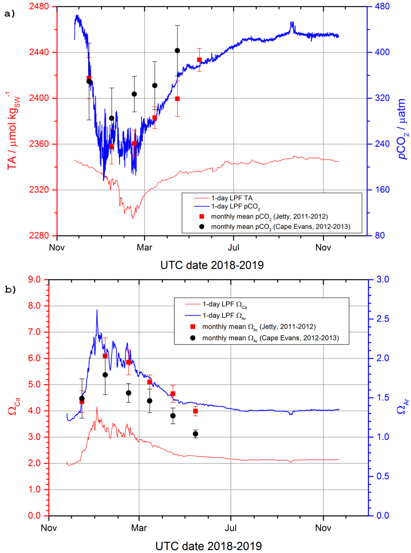
• to estimate the sensitivity of the carbonate system (total alkalinity (TA), partial pressure of carbon dioxide in seawater (pCO₂), and calcite and aragonite saturation states (Ω_Ca, Ω_Ar)), derived by direct measurements of physical and biogeochemical drivers at the coastal site.

2. Materials and Methods

2.1. Study Area: Location and Characteristics

The study was carried out in a coastal site of TNB, which is located on the western margin of the Ross Sea (Figure 1). TNB measures approximately 80 km × 30 km and stretches from the narrow peninsula of Cape Washington (74°44′ S 163°45′ E), in the north, to the floating tongue of the Drygalski glacier (64°43′ S 60°44′ W), arising from David Glacier [26] in the south. The bay comprises a tortuous continental shelf with numerous banks and trenches. The mean depth of the shelf is about 450 m, with greatest depths close to the coast and up to 1000 m depths in the adjacent basin. The orography of the region is responsible for determining its climate. Local katabatic winds often keep the area free of ice, causing temperature drops (surface seawater temperature range: −1.9, +1 °C) [27] and a delay in summer seawater stratification, and are also responsible for the formation and preservation of polynyas persisting during wintertime [28].

TNB is one of the source areas for DSW, the precursor for the AABW, which is produced on the Antarctic continental shelf, where winter cooling and salinification by sea ice formation produce shelf waters of sufficient density to sink to the deep ocean [20]. The strongest heat loss and salt injection occur in coastal polynyas, where persistent wind-driven export of sea ice allows for continuous sea ice formation [29]. Sea ice formation in the TNB polynya represents the local inputs contributing to the observed high salinity (absolute salinity values greater than 34.9 g kg⁻¹) of the DSW on the western Ross Sea continental shelf [19].

The seasonal sea ice coverage in TNB strongly impacts the cycling of chemical species and biological processes by restricting the CO₂ exchange between the air and the sea during winter and thus limits the equilibration of the Antarctic surface water with the overlying atmosphere. As a result of the heterotrophic activities, this surface water becomes supersaturated with CO₂ and undersaturated in terms of DO [30]. The carbonate system in the Ross Sea and the variability associated with different water masses were investigated in a summer campaign in 2008 [31], showing that the highest pH_T values in TNB (about 8.03 at 200 m of depth) are measured where waters are oversaturated (more than 1) in terms of both calcite and aragonite [32,33].

TNB is entirely covered by sea ice for at least 9 months of the year [26]. When the ice melts, phytoplankton blooms occur, which lead to big changes in the carbonate systems, also affecting local productivity of benthic ecosystems. The seasonality of phytoplankton production is generally characterized by a main peak occurring from the second half of December through to the beginning of January and eventually by a second late-summer bloom in February [34]. Phytoplankton bloom normally occurs when maximum irradiance is reached and there is enough energy to cause the ice to melt as well as to warm up and stabilize the upper layer of seawater. Irradiance values range from a maximum of 36 MJ m⁻² day^−l (equivalent to 70 E m⁻² day^−l of PAR) near the solstice of December to a minimum below 5 MJ m⁻² day^−l in the second half of February, in clear-sky conditions [34]. Under such conditions, thermal stratification occurs and nutrient depletion is very pronounced, with nutrients sometimes reaching concentration levels that might be limiting for phytoplankton growth [35]. Moreover, physical factors, such as the strong winds, play an important role in developing a phytoplankton system that, for TNB, shows a patchy distribution, causing a shift from an autotrophic community in areas close to the glaciers toward a heterotrophic community in the shallower layers of free ice areas [36].

2.2. The Underwater Observatory

The underwater observatory (Figure 2) consisted of a set of probes and sensors and 12 cages with biological samples mounted on a square metal frame (each side about 2 m; 100 kg in weight). By means of SCUBA diving, the system was deployed at about 25 m of depth under the ice pack in TNB (Figure 1) close to the Italian Mario Zucchelli Station (MZS) (latitude 74°41′23.887″ S; longitude 164°06′14.730″ E) on 15 November 2018.

For the environmental monitoring, three types of probes were used:

1—one pH meter (SeaFET V2, SEA-BIRD, Bellevue, WA, USA and a solid-state ion-sensitive field-effect transistor (ISFET)) probe for long-lasting time series of pH_T measurements;

2—one conductivity–temperature–depth probe (CTD, SBE37-SMP-ODO, SEA-BIRD, Bellevue, WA, USA) for direct measurement of p, t, C (from which indirect measures of S_P and ρ were derived), and DO;

3—six light and temperature sensors (HOBO UA-002-64, Pendant, Bourne, MA, USA), essentially dedicated to Ev measurement.

The pH meter and CTD probes were mounted directly on the metal frame and then hydraulically connected by a pumped duct in order to simultaneously analyze the same portion of water; light and temperature loggers were mounted on the top of the cages containing the biological samples, not analyzed in this study (Figure 2).

Prior to deployment, a preliminary testing activity in the laboratory (operational and mechanical checks) was performed on all probes and sensors. General metrological features of deployed probes are shown in

Table 1. Main metrological features of employed probes as reported by datasheets. Temperatures (*) were acquired but are not presented in this paper. CTD temperature values are the most reliable, thus indicated in the table and used in the paper. The symbol u_c indicates the available (or calculated) combined standard uncertainty. N.a.: not applicable

Probe Model	Quantity	Units	Accuracy	Stability	uc
SBE SeaFET V2	Total scale pH	---	±0.05 pHT	0.005 pHT month−1	0.06
	Temperature *	°C	n/a	n/a	n/a
CTD SBE37-SMP-ODO	Temperature	°C	±0.002	0.0002 month−1	0.023
	Pressure	dbar	±0.35	0.01 month−1	0.24
	Electrical Conductivity	mS cm−1	±0.003	0.003 month−1	0.032
	Dissolved oxygen	mL L−1	±0.07	0.0002 month−1	n/a
	Practical salinity	PSU	n/a	n/a	0.009
	Density	kg m−3	n/a	n/a	n/a
HOBO Pendant Logger	Illuminance	lux	n/a	n/a	n/a
	Temperature *	°C	±0.53 °C	n/a	n/a

, whereas values of accuracy and stability are reported as declared on the company datasheet. CTD and pH meters were both produced in 2018. Thus, for year-round acquisition, their values of accuracy and stability were assumed to fall within the validity of their calibration documents. The extreme environmental conditions at the study site led us to assess the stability of these instruments by using ad hoc methods: when possible, their stability was verified to the best of the available experimental capabilities (i.e., by applying pre- and post-deployment metrological checks performed in the laboratory; Figures S1–S3, Supplementary Materials); otherwise the calibration documents were used. It should be noted that the information provided by these documents is not in accordance with the current rules and standards governing the expression of measurement uncertainties [37] and its reliability, as a combined standard uncertainty associated with the quantity of interest, is partially neglected because of the lack of the associated coverage factor to the accuracy or error. Given that the accuracy of SeaFET has to be intended as a standard uncertainty (company’s private communication to G.R. and referring to previous in-field metrological characterization of a comparable CTD probe [38], the combined standard uncertainties u_c of the main quantities of interest are reported in Table 1 (values should be considered as conservative, including the time stability contribution calculated at the end of a 12-month deployment).

2.3. Data Collection, Processing, and Analyses

2.3.1. Underwater Observatory Data

Before being deployed, all probes were synchronized to UTC time and programmed to acquire one measure per hour (at the beginning of each hour). Simultaneous data acquisition started on 25 November 2018 (04:00 UTC) and ended 361.7 days later, on 21 November 2019 (21:00 UTC), allowing a continuous hourly time series of 8682 recordings to be logged for each parameter measured by CTD and SeaFET probes (light-intensity measurements lasted about 4 days less, due to the early recovery of the cages housing the HOBO sensors). All the acquired data satisfied quality control by the instruments employed. For pH_T measurements, 2 weeks prior to the deployment in the laboratory, the SeaFET measuring cell was filled with seawater samples collected from the field and filtered for preliminary checks to be carried out. Once the probes were deployed, data acquisition started after the recommended conditioning period (24 h) needed by the instrument for recording optimal data (see [39] and Supplementary Materials for further details on probe preparation).

Once recovered, all probes were inspected to check that no hardware anomalies had occurred during data acquisition. Then, data were downloaded to check the presence of spikes, anomalous noise, or trends before being analyzed. For pH data, the pH_T signal measured by one of the two different SeaFET reference electrodes (the internal (INT) one) showed very low and spiky values, so failing quality control analyses. This was probably due to the potassium chloride electrolyte escaping from the INT reference, causing a failure in the pH_T internal output (company’s private communication to G.R.). Thus, data from the SeaFET_INT sensor are not reported in this paper. The SeaFET external (EXT) sensor, however, was completely unaffected by the INT sensor behavior and acquired pH_T values free of anomalies. To provide the most accurate and stable pH_T data [39], the EXT sensor data were post-processed by applying a salinity–temperature correction based on CTD data through the SBE-UCI software (v. 2.0.2)

CTD data were processed by using company software (SBE-Seaterm V2, v.2-7-0-108). Relationships and charts were realized by using Ocean Data View [40]. In particular, for pressure measures, fast Fourier transform (FFT) analysis was applied to calculate principal tidal constituents (principal solar semidiurnal (S₂), principal lunar semidiurnal (M₂), larger lunar elliptic semidiurnal (N₂), principal lunisolar diurnal (K₁), principal solar diurnal (P₁), principal lunar diurnal (O₁), larger lunar elliptic (Q₁)) and their relative periods.

TA was estimated by applying the formula from [41] based on measured sea surface temperature and practical salinity. pCO₂, Ω_Ca, and Ω_Ar were calculated by TA and pH_T using CO2Calc software (v. 4.0.9, U.S. Geological Survey [42]; see Supplementary Materials for methodologies). Because of the lack of proper analytical instruments at the Italian base and the very short time spent at MZS (2 months per year) during the whole study period (12 months), spectrophotometric measurements for the pH and Winkler for dissolved oxygen were not used to validate data from the sensors of pH and DO.

2.3.2. Satellite Data

Data of sea ice concentration (SIC) were downloaded from the Copernicus Marine Environment Monitoring Service data base (CMEMS, https://marine.copernicus.eu) to complement in situ physico-chemical parameters (Figure 3). SIC is reported as a fraction from 0 to 1, where 0 corresponds to the absence of ice and 1 is the maximum ice coverage for the region. The CMEMS product used for the analyses had the following features:

• name: SST_GLO_SST_L4_NRT_OBSERVATIONS_010_001;
• type of data: daily mean satellite observations from 1 January 2007 (near-real-time);
• spatial resolution: 0.05° × 0.05° (surface only, approx. 1.6 km × 5.6 km);
• product level: L4, i.e., a product for which a temporal averaging method or an interpolation procedure is applied to fill out missing data values. Temporal averaging is performed on a monthly basis.

Satellite chlorophyll-a data were also obtained from the CMEMS database to complement observed parameters (DO and E_V). Data are expressed as mass concentration of Chl-a in seawater (mg m⁻³) (Figure 3). Analogously, the CMEMS product used for the analyses had the following features:

• name: OCEANCOLOUR_GLO_CHL_L3_REP_OBSERVATIONS_009_085;
• type of data: daily observations of mass concentration of Chl-a in seawater (mg m⁻³); daily mean reprocessed from 1997;
• spatial resolution of data: 4 km × 4 km (surface only);
• product level: L3, i.e., data are the daily composite products as obtained by merging all the ocean satellite passages.

3. Results

3.1. Physical and Biological Environment

Monthly and annual values for measured (pH_T, p, t, S_P, ρ, DO, E_V) variables for the period November 2018–November 2019 are displayed in

Table 2. Mean annual and monthly values, with their associated standard deviation (s.d.) (i.e., the measure of dispersion of the values over time), of total scale pH (pH_T), temperature (t), practical salinity (S_P), density (ρ), dissolved oxygen (DO), illuminance (E_V), total alkalinity (TA), pCO₂, Ω_Ca, and Ω_Ar at the study site between November 2018 and November 2019. Values indicated by * were calculated from temperature and salinity measures [42] and ** were calculated using CO2Calc, K1 and K2 dissociation constants estimated by [43], total boron from [44], and KHSO4 dissociation constant by [45].

Annual	pHT	p dbar	t °C	Sp PSU	ρ kg m−3	DO mL L−1	Ev lux	TA * μmol kgSW−1	pCO2 ** μatm	ΩCa **	ΩAr **
mean	8.09 ± 0.08	25.10 ± 0.19	−1.63 ± 0.56	34.61 ± 0.24	1027.98 ± 0.20	7.42 ± 0.71	4	2336 ± 13	367 ± 74	2.44 ± 0.46	1.53 ± 0.29
median	8.05	25.07	−1.91	34.72	1028.06	7.17	0	2340	395	2.22	1.39
min	7.97	24.57	−1.95	33.72	1027.25	6.61	0	2292	176	1.91	1.20
max	8.35	25.76	1.08	34.87	1028.20	10.61	201	2350	466	4.42	2.78
range	0.38	1.19	3.03	1.15	0.95	4.00	201	59	290	2.51	1.58
Monthly
Dec-18	8.09 ± 0.09	25.07 ± 0.20	−1.09 ± 0.45	34.73 ± 0.02	1028.05 ± 0.03	8.04 ± 0.84	0	2340 ± 3	355 ± 79	2.55 ± 0.54	1.60 ± 0.34
Jan-19	8.24 ± 0.04	25.09 ± 0.20	−0.13 ± 0.37	34.50 ± 0.20	1027.82 ± 0.15	8.85 ± 0.54	8	2324 ± 9	242 ± 24	3.41 ± 0.27	2.14 ± 0.17
Feb-19	8.24 ± 0.03	25.14 ± 0.19	−1.31 ± 0.15	33.99 ± 0.11	1027.47 ± 0.09	8.26 ± 0.26	12	2305 ± 5	240 ± 21	3.13 ± 0.19	1.96 ± 0.12
Mar-19	8.16 ± 0.02	25.12 ± 0.18	−1.74 ± 0.18	34.35 ± 0.07	1027.77 ± 0.06	7.72 ± 0.11	21	2323 ± 4	291 ± 16	2.74 ± 0.11	1.72 ± 0.07
Apr-19	8.09 ± 0.02	25.11 ± 0.17	−1.89 ± 0.02	34.54 ± 0.05	1027.93 ± 0.04	7.39 ± 0.09	3	2333 ± 2	353 ± 18	2.39 ± 0.09	1.50 ± 0.05
May-19	8.07 ± 0.01	25.14 ± 0.19	−1.91 ± 0.00	34.61 ± 0.02	1027.98 ± 0.02	7.24 ± 0.05	0	2337 ± 1	379 ± 5	2.27 ± 0.02	1.42 ± 0.01
Jun-19	8.05 ± 0.01	25.12 ± 0.20	−1.92 ± 0.01	34.69 ± 0.06	1028.05 ± 0.05	7.15 ± 0.05	0	2341 ± 3	398 ± 8	2.21 ± 0.02	1.39 ± 0.01
Jul-19	8.03 ± 0.00	25.10 ± 0.22	−1.93 ± 0.00	34.74 ± 0.02	1028.09 ± 0.02	6.98 ± 0.06	0	2344 ± 1	419 ± 5	2.14 ± 0.02	1.34 ± 0.01
Aug-19	8.03 ± 0.00	25.09 ± 0.20	−1.93 ± 0.00	34.74 ± 0.02	1028.10 ± 0.02	6.90 ± 0.03	0	2344 ± 1	423 ± 3	2.13 ± 0.01	1.34 ± 0.01
Sep-19	8.02 ± 0.01	25.03 ± 0.17	−1.92 ± 0.00	34.81 ± 0.02	1028.15 ± 0.02	6.80 ± 0.07	0	2347 ± 1	435 ± 6	2.11 ± 0.02	1.32 ± 0.02
Oct-19	8.03 ± 0.00	25.04 ± 0.18	−1.92 ± 0.01	34.82 ± 0.01	1028.16 ± 0.01	6.81 ± 0.02	0	2348 ± 1	430 ± 2	2.14 ± 0.01	1.34 ± 0.01
Nov-19	8.03 ± 0.00	25.09 ± 0.19	−1.88 ± 0.03	34.79 ± 0.01	1028.13 ± 0.01	6.82 ± 0.04	0	2346 ± 1	430 ± 2	2.14 ± 0.01	1.34 ± 0.01

.

Regarding t (Figure 4a), values showed an annual variation of 3.03 °C, with a mean of −1.63 ± 0.56 °C. Warmer temperatures occurred in January with −0.13 ± 0.37 °C and values above 0 °C (up to 1.08 °C) during part of the day when the maximum solar irradiance was reached, between 8 a.m. and 2 p.m. On the other hand, the coldest months were July and August, with a very stable temperature of −1.93 °C (minimum equal to −1.95 °C).

S_P and ρ values showed similar trends (Figure 4b,c), with the lowest values in February 2019 (33.72 PSU and 1027.25 kg m⁻³, respectively). The highest values (34.87 PSU and 1028.20 kg m⁻³) occurred in September 2019.

The annual mean value for DO (Figure 4d) was 7.42 ± 0.71 mL L⁻¹ (mean saturation equal to 88%), with the maximum value in January 2019, with 10.61 mL L⁻¹ (133%), and the minimum, with 6.61 mL L⁻¹ (78%), recorded in September 2019. Between December 2018 and February 2019, the DO signal reached the highest values, whereas the lowest were recorded at the end of data acquisition between September and November 2019: 6.80 ± 0.07 mL L⁻¹ and 6.82 ± 0.04 mL L⁻¹, respectively.

Overall the pattern of measured pH_T variations in the 12 months of data (Figure 4e) revealed the highest values between January and March 2019 (8.24 ± 0.04 and 8.16 ± 0.02) (mean ± s.d.) (Table 2), with a maximum value of 8.35 recorded in January 2019 and low values between July and November 2019 (8.05 ± 0.01 and 8.03 ± 0.00), with a minimum value of 7.97 at the beginning of data acquisition, in November 2018. The annual pH_T trend exhibited limited hourly variations, with an annual mean of 8.09 ± 0.08.

E_v data (Figure 4f) revealed minimum monthly mean values between January and April 2019 (up to 21 lux), with the hourly peak recorded at the beginning of March (201 lux). During the summer months, E_v showed daily fluctuations, with the highest values between 00.00 and 5 a.m.

Values of p showed an annual mean of 25.10 ± 0.19 dbar, with a minimum of 24.57 dbar and a maximum of 25.76 dbar recorded in February and April, respectively. Data on pressure were converted into depth (m) values (SBE Application Note, 2002). The experimental station being anchored to the bottom, the CTD pressure sensor was subjected to tidal effects (see Figure 5a) and the maximum tidal span was about 1.2 m large. Then, by applying FFT post-processing of the signal from pressure data, principal tidal constituents (S₂, M₂, N₂, K₁, P₁, O₁, Q₁) and their period, occurring during the study, were obtained and compared with the values reported from literature for the central Ross Sea Ice Shelf (Figure 5b).

Regarding relationships among t, S_P, and density (expressed as sigma-t density σ_t, i.e., σ_t − 1000 kg m⁻³, data showed that, in the study site, seawater density was mainly driven by practical salinity rather than temperature differences (for t = −1.9 °C, highest salinity in the range of 34.7–34.85 PSU and highest density in the range of 28.078–28.190 kg m⁻³; for t = −1.45 °C, lowest salinity in the range of 33.75–33.9 PSU and lowest density in the range of 27.296–27.408 kg m⁻³) (Figure 6).

Annual SIC and Chl-a trends from satellite data were compared with experimental values of DO and E_V (Figure 7). The lowest SIC values (sea ice area fraction equal to 0) were recorded in December 2018 and February 2019, whereas the maximum peaks of the sea ice area fraction (greater than 0.8) were recorded in July and August 2019 (Figure 7a). Data on Chl-a (Figure 7b) revealed that the maximum mass concentration value, 0.2–1.1 mg m⁻³, occurred from December 2019 to the first half of March 2019 and at the end of November 2019, in correspondence to the lowest sea ice area fractions. On comparing the trends of all these parameters, it was clear that DO fully phased with the algal bloom (Chl-a trend) during the summer season (Figure 7c). DO was the parameter with a fast response time, displaying the highest values (i.e. supersaturation) in correspondence to the maximum Chl-a concentrations. Differently, E_V showed a delayed trend with respect to Chl-a values, but with the highest illuminance (greater than 50 lux) in correspondence to the lowest sea ice fractions (February and March 2019) (Figure 7a,d) with a shift, especially for the first peak, probably due to the local variability of sea ice coverage.

For the summer period (January–April 2019), when DO and Chl-a revealed the maximum values, DO was plotted versus both t and S_P (Figure 8). Qualitative data clearly revealed the monotone trend of DO values as a positive function of t: the lowest DO data, in the range 7.210–7.636 mL L⁻¹, were recorded at t close to −1.9 °C, whereas the highest DO values, in the range 10.2–10.6 mL L⁻¹, occurred at an increased temperature (0.2 °C) and the maximum pH_T values of 8.3 (Table 2).

Finally, no significative relationship was found between pH_T and tidal height for the study period.

3.2. Calcification Environment

To explore how the calcification environment varied over time in the shallow coastal site of TNB and to evaluate the influence of biological activities, carbon parameters (TA, pCO₂, Ω_Ca, Ω_Ar) were calculated for the period of investigation. In addition, to validate the data, our estimations from the study site were plotted with data from nearby coastal locations in McMurdo Sound (Jetty and Cape Evans) collected in 2011–2012 and 2012–2013, respectively. All values are reported in Table 2 and plotted in Figure 9.

The trend of pCO₂ was comparable to that of TA (Figure 9a), with minimum peaks recorded in February 2019 (pCO₂: 240 ± 21 μatm; TA: 2305 ± 5 μmol kg_SW⁻¹), but was in contrast to the measured pH_T trend (max pH_T: 8.24 ± 0.03; Figure 4a). Monthly mean calculated pCO₂ values ranged between 240 and 435 μatm. The highest values (greater than 400 μatm) were recorded during 42% of the study period (July–November 2019), whereas values in the range of 300–400 μatm and 200–300 μatm were recorded during 33.3% and the remaining during 25.1% of the study period (January–March 2019).

Saturation states of both calcite and aragonite showed their highest values in January 2019 (Ω_Ca: 3.41 ± 0.27; Ω_Ar: 2.14 ± 0.17), in correspondence to the maximum value of DO (8.85 ± 0.549 mL L⁻¹), and the minimum values in September 2019 (Ω_Ca: 2.11 ± 0.02; Ω_Ar: 1.32 ± 0.02), at the end of phytoplankton activity (Figure 9b). Both Ω_Ca and Ω_Ar showed reasonable annual trends, with a significative decline from summer to autumn/winter. Experimental results are also qualitatively comparable, with measurements performed at McMurdo, especially with those during 2011–2012. No undersaturation estimates were recorded for the 12-month period for both calcite and aragonite saturation states.

4. Discussion

Mooring sites are well spread in Antarctica, recording physico-chemical seawater data in deep sites as well as describing Antarctic current dynamics [47,48,49] of sites, including Ross Sea and Terra Nova Bay [50,51,52]. With the exception of a few sites, such as Arthur Harbor (Palmer Station Antarctic Peninsula) [53], King George Island [54], and McMurdo Sound (western Ross Sea) [14,46,55], to date, there are not many underwater annual in-continuum measurements in coastal shallow sites, representing very unique and dynamic environments.

Prohibitive and unpredictable environmental conditions put instruments at risk, but such observatories are extremely important because of the need for data acquisition in polar areas due to the rapidity of the occurring changes [1,2]. The data presented here are from the underwater observatory (Figure 2), anchored on the sea bottom at 25 m of depth under the ice pack, which allowed in situ seawater parameters to be recorded over 12 months (Figure 4, Table 2). Despite the limitation of this study to a single station, the first successful all-year-round underwater monitoring allowed high-temporal-resolution data to be produced describing physico-chemical and biological processes occurring in a shallow coastal site at TNB. The area has been studied for the past 30 years by Italian Antarctic researchers [26,56], but in situ 12-month physico-chemical variability has never been previously monitored.

Our findings reveal that, between November 2018 and November 2019, the trends of physico-chemical parameters reflected the seasonality of the environment. Major changes occurred between December and March, probably driven by two main processes: ice melting and biological activities.

The temperature remained stable at −1.9 °C for 7 months, between April and November, and displayed a variability of 3.03 °C across a short time frame between December and March. Temperature represents one of the major drivers of biological processes by inducing the activation of physiological activities in most of the local ecosystems [57,58]. Furthermore, the temperature increase, determined by the sunray angles, represented the trigger for sea ice melting, even though it did not represent the major driver for density, confirming an important role of the polynyas and dense shelf waters (DSW) originating in coastal areas and detectable on a very local scale [20].

Density was mainly driven by practical salinity (i.e., lowest salinity = lowest seawater density), reaching the minimum value of 33.72 PSU in February 2019, in correspondence to minimum SIC (sea ice area fraction equal to 0) and low temperatures (−1.35 °C). Interestingly, the most saline waters (S_P greater than 34.8 PSU) occurred between September and November 2019, when the sea ice coverage was the highest (SIC greater than 0.8). Given the position of the study site (the observatory is located at 25 m of depth), this saline water can be attributed to brine rejection from sea ice formation in the TNB polynya and also to remote inputs, as salt content might be advected toward TNB by coastal currents (DSW) [20]. These increases in salinity and density, associated with the sea ice coverage, also drive convection and mixing and influence sea ice motion.

In fact, the sea ice motion was clearly visible between December 2018 and February 2019, with SIC values oscillating from 0 to a maximum peak of 0.4 and back to 0 again, as a result of a combination of stresses from the atmosphere and the ocean [59,60]. This motion was determined by forces applied both on the ice surface by katabatic wind stress as well as at the base by ocean currents, including tides [61]. Gradients in tidal currents, causing periodic divergence and convergence of the ice pack [62], were responsible in determining the biggest SIC range (0–0.4) during summer (January 2019). Noticeably, when local tidal effects on sea ice are coupled with the seasonal cycle (autumn–winter net ice production and spring–summer net ice loss) and with the larger-scale advection of water masses (determined by the DSW), the turnover between sea ice production and loss has a substantial effect on the large-scale ocean and sea ice state [63]. Tide-induced signals provide insight into the processes by which the oceans can affect ice sheet mass balance and dynamics [64]; thus high-temporal-resolution data from underwater observatories represent an important tool for improving understanding of the role of tides in ice sheet dynamics and for predicting the future ice sheet mass budget and sea-level rise.

The seasonal sea ice coverage is accompanied by the rise or decline in biological activities [6,31] which, also for the site, were intensified at ice melting [65]. In December, the sea ice melting exerted a possible influence on controlling the carbonate system chemistry of the site both directly through dilution processes and indirectly by favoring the development of phytoplankton blooms, as observed in McMurdo Sound [46]. Differently from other studies considering mixed layers [66], at the shallow coastal site in TNB, the increase in pH_T recorded at the end of the year (the maximum peak during this period with a value of 8.35) was accompaigned by maximum values for both estimated saturation states (Ω_Ca = 4.42; Ω_Ar = 2.78). While pCO₂ displayed the minimum value, with 176 μatm, and a dilution of TA was recorded. In accordance with processes observed in McMurdo Sound (western Ross Sea), the variation in the thickness and attenuation of sea ice, starting in December, might have doubled the effect on the measured pH_T due to photosynthesis [14,52]. This would explain the highest pH_T value recorded at the beginning of the season. In the meantime, the DO peak (oversaturation: 133%) occurring in December was due to the first phytoplankton bloom (i.e., sympagic algae) of the season, with a Chl-a mass concentration of 0.3 mg m⁻³ and the start of its photosynthetic activity. In fact, sympagic algae are released in small quantities from sea ice before its breakup and, in a short time frame, as a strong bloom during and soon after the melting of sea ice [67,68,69]. The photosynthetic performance of phytoplankton reveals a general adaptation to low-light regimes, characterized by high values of photosynthetic efficiency and also by low-temperature adaptation of the growth performance [70].

The greatest change in the carbonate system occurred in January, confirming the effect of melting freshwater (SIC range: 0–0.1), which also affected TA, resulting in a minimum of 2292 μmol kg_SW⁻¹ [66,71]. pH_T showed a second positive peak with 8.33, and low-estimated pCO₂ concentrations of approx. 200 μatm were observed. Probably due to the highest quality of light available at 25 m (approx. 50 lux), because of the free ice coverage (SIC = 0), Chl-a showed the maximum mass concentration (approx. 1 mg m⁻³). Thus, the maximum photosynthetic activities would be expected, but, interestingly, the DO trend declined (mean saturation: 78%) as an indication of a post-bloom effect. Both derived saturation states also declined from December to February, stabilizing at minimum constant values (greater than 1 mL L⁻¹) in July 2019. During summer months, the variability of the surface carbonate system properties at this shallow site was primarily controlled by biological activities [20]. These include not only phytoplankton blooms, changes in species composition depending on sea ice influence, current, and water mixing [68], but also physiological processes of bacteria [72] and, on a macro scale, of benthic ecosystems (i.e., respiration, photosynthesis, calcification). Benthic ecosystems of the site were primarily characterized by calcifying filter feeders [65,73], sessile or vagile, such as bryozoans, corals, sponges, molluscs, and echinoderms. After the ice melt, an abundant quantity of food becomes available in a few hours to these consumers, which adopt a more specialized diet and increased feeding rate [74,75]. This was observed both at the level of the entire food web and in species analyzed from the same site during the two-year investigation [63]. Thus, considering the abundance of califiers at the site, DO, pCO₂, and saturation state reduction can be due to intensification of their physiological activities, such as growth (i.e., calcification causing carbonate consumption) other than reproductive activities during summer months [58,76].

Under the rapidly progressing climate change, the complexity of processes and their variability occurring at local scales in a very short time frame call for more data collection. Even the local character of our study, TNB, is where the DSW, the precursor for the AABW, orginate and bring information on water masses from local coastal systems [20]. The increase in anthropogenic CO₂ storage in the AABW recorded in the past 40 years was accompained by a long-term change in total carbon concentration due to anthropogenic CO₂ uptake of the different formation regions [33]. All these changes were modulated by significant interannual to multi-annual variability associated with variations in physico-chemical properties (i.e., temperature, practical salinity, DO, TA, pCO₂) orginating at local other than regional scales involving the ecosystems. Thus, we hope in the increase of in situ observatories, representing powerful tools for recording and monitoring rapidly occurring changes in shallow and deep polar environments [2,77] as well as their cascading effects on polar biodiversity [9,58,78].

References

1. Meredith, M.P.; Schofield, O.; Newman, L.; Urban, E.; Sparrow, M. The vision for a Southern Ocean Observing System. Curr. Opin. Environ. Sustain. 2013, 5, 306–313. [Google Scholar] [CrossRef]
2. Meredith, M.P.; Sommerkorn, M.; Cassotta, S.; Derksen, C.; Ekaykin, A.; Hollowed, A.; Kofinas, G.; Mackintosh, A.; Mel-bourne-Thomas, J.; Muelbert, M.M.C.; et al. IPCC Special Report on the Ocean and Cryosphere in a Changing Climate; Pörtner, H.-O.D.C., Roberts, V., Masson-Delmotte, P., Zhai, M., Tignor, E., Poloczanska, K., Mintenbeck, A., Alegría, M., Nicolai, A., Okem, J., et al., Eds.; 2019; in press. [Google Scholar]
3. Collins, W.J.; Fry, M.M.; Yu, H.; Fuglestvedt, J.S.; Shindell, D.T.; West, J.J. Global and regional temperature-change potentials for near-term climate forcers. Atmos. Chem. Phys. Discuss. 2013, 13, 2471–2485. [Google Scholar] [CrossRef] [Green Version]
4. von Schukmann, K.; Le Traon, P.-Y.; Smith, N.; Pascual, A.; Djavidnia, S.; Gattuso, J.-P.; Grégoire, M.; Nolan, G. Co-pernicus Marine Service Ocean State Report. J. Oper. Ocean 2020, 13, S1–S172. [Google Scholar]
5. Berger, A.; Yin, Q.; Nifenecker, H.; Poitou, J. Slowdown of global surface air temperature increase and acceleration of ice melting. Earth’s Futur. 2017, 5, 811–822. [Google Scholar] [CrossRef]
6. Convey, P.; Peck, L.S. Antarctic environmental change and biological responses. Sci. Adv. 2019, 5, eaaz0888. [Google Scholar] [CrossRef] [Green Version]
7. Barnes, D.K.A. Iceberg killing fields limit huge potential for benthic blue carbon in Antarctic shallows. Glob. Chang. Biol. 2016, 23, 2649–2659. [Google Scholar] [CrossRef] [Green Version]
8. Barnes, D.K.A. Polar zoobenthos blue carbon storage increases with sea ice losses, because across-shelf growth gains from longer algal blooms outweigh ice scour mortality in the shallows. Glob. Chang. Biol. 2017, 23, 5083–5091. [Google Scholar] [CrossRef]
9. Gutt, J.; Isla, E.; Bertler, A.N.; Bodeker, G.E.; Bracegirdle, T.J.; Cavanagh, R.D.; Comiso, J.C.; Convey, P.; Cummings, V.; De Conto, R.; et al. Cross-disciplinarity in the advance of Antarctic ecosystem research. Mar. Gen. 2017, 37, 1–17. [Google Scholar] [CrossRef]
10. Henley, S.F.; Schofield, O.M.; Hendry, K.R.; Schloss, I.R.; Steinberg, D.K.; Moffat, C.; Peck, L.S.; Costa, D.P.; Bakker, D.C.; Hughes, C.; et al. Variability and change in the west Antarctic Peninsula marine system: Research priorities and opportunities. Prog. Oceanogr. 2019, 173, 208–237. [Google Scholar] [CrossRef] [Green Version]
11. Gutt, J.; Bertler, N.; Bracegirdle, T.J.; Buschmann, A.; Comiso, J.; Hosie, G.; Isla, E.; Schloss, I.R.; Smith, C.R.; Tournadre, J.; et al. The Southern Ocean ecosystem under multiple climate change stresses—An integrated circumpolar assessment. Glob. Chang. Biol. 2015, 21, 1434–1453. [Google Scholar] [CrossRef] [Green Version]
12. Hoffmann, G.E.; Smith, J.E.; Johnson, K.S.; Send, U.; Levin, L.A.; Micheli, F.; Paytan, A.; Price, N.N.; Peterson, B.; Takeshita, Y.; et al. High-frequency dy-namics of ocean pH: A multi-ecosystem comparison. PLoS ONE 2012, 6, e28983. [Google Scholar]
13. Bindoff, N.L.; Cheung, W.W.L.; Kairo, J.G.; Arístegui, J.; Guinder, V.A.; Hallberg, R.; Hilmi, N.; Jiao, N.; Karim, M.S.; Levin, L.; et al. Changing Ocean, Marine Eco-systems, and Dependent Communities. In IPCC Special Report on the Ocean and Cryosphere in a Changing Climate; Pörtner, H.O.D.C., Roberts, V., Masson-Delmotte, P., Zhai, M., Tignor, E., Poloczanska, K., Mintenbeck, A., Alegriía, M., Nicolai, A., Okem, J., Eds.; 2019; in press. [Google Scholar]
14. Matson, P.G.; Washburn, L.; Martz, T.R.; Hofmann, G.E. Abiotic versus Biotic Drivers of Ocean pH Variation under Fast Sea Ice in McMurdo Sound, Antarctica. PLoS ONE 2014, 9, e107239. [Google Scholar] [CrossRef]
15. Deppeler, S.L.; Davidson, A.T. Southern Ocean Phytoplankton in a Changing Climate. Front. Mar. Sci. 2017, 4. [Google Scholar] [CrossRef] [Green Version]
16. Caldeira, K.; Duffy, P.B. The role of Southern Ocean in uptake and storage of anthropogenic carbon dioxide. Science 2000, 287, 620–622. [Google Scholar] [CrossRef] [PubMed] [Green Version]
17. Sabine, C.L.; Feely, R.A.; Gruber, N.; Key, R.M.; Lee, K.; Bullister, J.L.; Wanninkhof, R.; Wong, C.S.; Wallace, D.W.R.; Tilbrook, B.; et al. The Oceanic Sink for Anthropogenic CO2. Science 2004, 305, 367–371. [Google Scholar] [CrossRef] [Green Version]
18. Budillon, G.; Pacciaroni, M.; Cozzi, S.; Rivaro, P.; Catalano, G.; Ianni, C.; Cantoni, C. An optimum multiparameter mixing analysis of the shelf waters in the Ross Sea. Antarct. Sci. 2003, 15, 105–118. [Google Scholar] [CrossRef] [Green Version]
19. Orsi, A.H.; Wiederwhol, C.L. A recount of Ross Sea waters. Deep Sea Res. Part II Top Stud. Ocean 2009, 56, 778–795. [Google Scholar] [CrossRef]
20. Silvano, A.; Foppert, A.; Rintoul, S.R.; Holland, P.R.; Tamura, T.; Kimura, N.; Castagno, P.; Falco, P.; Budillon, G.; Haumann, F.A.; et al. Recent recovery of Antarctic Bottom Water formation in the Ross Sea driven by climate anomalies. Nat. Geosci. 2020, 13, 780–786. [Google Scholar] [CrossRef]
21. Barnes, D. Antarctic sea ice losses drive gains in benthic carbon drawdown. Curr. Biol. 2015, 25, R789–R790. [Google Scholar] [CrossRef] [Green Version]
22. Barnes, D.K.; Ireland, L.; Hogg, O.T.; Morely, S.; Enederlein, P.; Sands, C.J. Why is the Southern Orkney Island shelf (the world’s first high seas marine protected area) a carbon immobilization hotspot? Glob. Chang. Biol. 2016, 22, 1110–1120. [Google Scholar] [CrossRef]
23. Doney, S.C.; Ruckelshaus, M.; Duffy, J.E.; Barry, J.P.; Chan, F.; English, C.A.; Galindo, H.M.; Grebmeier, J.M.; Hollowed, A.B.; Knowlton, N.; et al. Climate Change Impacts on Marine Ecosystems. Annu. Rev. Mar. Sci. 2012, 4, 11–37. [Google Scholar] [CrossRef] [PubMed] [Green Version]
24. Roleda, M.Y.; Boyd, P.W.; Hurd, C.L. Before ocean acidification: Calcifier chemistry lessons. J. Phycol. 2012, 48, 840–843. [Google Scholar] [CrossRef] [PubMed]
25. Cyronak, T.; Schulz, K.G.; Jokiel, P.L. The Omega myth: What really drives lower calcification rates in an acidifying ocean. ICES J. Mar. Sci. 2016, 73, 558–562. [Google Scholar] [CrossRef] [Green Version]
26. Faranda, F.M.; Guglielmo, L.; Ianora, A. The Italian Oceanographic Cruises in the Ross Sea (1987-95): Strategy, General Con-sideration and Description of the sampling sites. In Ross Sea Ecology; Faranda, F.M., Guglielmo, L., Ianora, A., Eds.; Springer: Berlin/Heidelberg, Germany, 2000; pp. 1–14. [Google Scholar]
27. Illuminati, S.; Annibaldi, A.; Romagnoli, T.; Libani, G.; Antonucci, M.; Scarponi, G.; Totti, C.; Truzzi, C. Distribution of Cd, Pb and Cu between dissolved fraction, inorganic particulate and phytoplankton in seawater of Terra Nova Bay (Ross Sea, Antarctica) during austral summer 2011–12. Chemosphere 2017, 185, 1122–1135. [Google Scholar] [CrossRef]
28. Colacino, M.; Piervitali, E.; Grigioni, P. Climatic Characterization of the Terra Nova Bay Region. In Ross Sea Ecology; Faranda, F.M., Guglielmo, L., Ianora, A., Eds.; Springer: Berlin/Heidelberg, Germany, 2000; pp. 15–26. [Google Scholar]
29. Nihashi, S.; Ohshima, K.I. Circumpolar Mapping of Antarctic Coastal Polynyas and Landfast Sea Ice: Relationship and Variability. J. Clim. 2015, 28, 3650–3670. [Google Scholar] [CrossRef]
30. Sweeney, C. The annual cycle of surface water CO2 And O2 in the Ross Sea: A model for gas exchange on the continental shelves of Antarctica. In Biogeochemistry of the Ross Sea; DiTullio, G.R., Dunbar, R.B., Eds.; American Geophysical Union: Washington, DC, USA, 2003; pp. 295–312. [Google Scholar]
31. Rivaro, P.; Messa, R.; Ianni, C.; Magi, E.; Budillon, G. Distribution of total alkalinity and pH in the Ross Sea (Antarctica) waters during austral summer. Polar Res. 2014, 33, 20403. [Google Scholar] [CrossRef] [Green Version]
32. Pardo, P.C.; Tilbrook, B.; Langlais, C.; Trull, T.W.; Rintoul, S.R. Carbon uptake and biogeochemical change in the Southern Ocean, south of Tasmania. Biogeosciences 2017, 14, 5217–5237. [Google Scholar] [CrossRef] [Green Version]
33. Mahieu, L.; Monaco, C.L.; Metzl, N.; Fin, J.; Mignon, C. Variability and stability of anthropogenic CO2 in Antarctic Bottom Water observed in the Indian sector of the Southern Ocean, 1978–2018. Ocean Sci. 2020, 16, 1559–1576. [Google Scholar] [CrossRef]
34. Lazzara, L.; Nardello, I.; Ermanni, C.; Mangoni, O.; Saggiomo, V. Light environment and seasonal dynamics of microalgae in the annual sea ice at Terra Nova Bay, Ross Sea, Antarctica. Antarct. Sci. 2007, 19, 83–92. [Google Scholar] [CrossRef] [Green Version]
35. Guglielmo, L.; Carrada, G.C.; Catalano, G.; Dell’Anno, A.; Fabiano, M.; Lazzara, L.; Mangoni, O.; Pusceddu, A.; Saggiomo, V. Structural and functional properties of sympagic communities in the annual sea ice at Terra Nova Bay (Ross Sea, Antarctica). Polar Biol. 2000, 23, 137–146. [Google Scholar] [CrossRef]
36. Umani, S.F.; Monti, M.; Bergamasco, A.; Cabrini, M.; De Vittor, C.; Burba, N.; Del Negro, P. Plankton community structure and dynamics versus physical structure from Terra Nova Bay to Ross Ice Shelf (Antarctica). J. Mar. Syst. 2005, 55, 31–46. [Google Scholar] [CrossRef]
37. JCGM 100:2008—Evaluation of Measurement Data—Guide to the Expression of Uncertainty in Measurement. Available online: https://ncc.nesdis.noaa.gov/documents/documentation/JCGM_100_2008_E.pdf (accessed on 6 January 2021).
38. Raiteri, G.; Bordone, A.; Ciuffardi, T.; Pennecchi, F. Uncertainty evaluation of CTD measurements: A metrological approach to water-column coastal parameters in the Gulf of La Spezia area. Measurement 2018, 126, 156–163. [Google Scholar] [CrossRef]
39. SBE Technical Note, Best Practices for the SeaFET V2: Optimizing pH Data Quality. Available online: https://repository.oceanbestpractices.org/handle/11329/876 (accessed on 6 January 2021).
40. Schlitzer, R. Ocean Data View. Available online: Odv.awi.de (accessed on 5 February 2021).
41. Lee, K.; Tong, L.T.; Millero, F.J.; Sabine, C.L.; Dickson, A.G.; Goyet, C.; Park, G.-H.; Wanninkhof, R.; Feely, R.A.; Key, R.M. Global relationships of total alkalinity with salinity and temperature in surface waters of the world’s oceans. Geophys. Res. Lett. 2006, 33, 19605. [Google Scholar] [CrossRef] [Green Version]
42. Robbins, L.L.; Hansen, M.E.; Kleypas, J.A.; Meylan, S.C. CO2calc—A User-friendly Seawater Carbon Calculator for Windows, Max OS X, and iOS (iPhone); U.S. Geological Survey Open-File Report 2010–1280; U.S. Geological Survey: St. Petersburg, FL, USA, 2010.
43. Roy, R.N.; Roy, L.N.; Vogel, K.M.; Porter-Moore, C.; Pearson, T.; Good, E.C.; Millero, F.J.; Campbell, D.M. The dissociation constants of carbonic acid in seawater at salinities 5 to 45 and temperatures 0 to 45 °C. Mar. Chem. 1993, 44, 249–267. [Google Scholar] [CrossRef]
44. Uppström, L.R. The boron/chlorinity ratio of deep-sea water from the Pacific Ocean. Deep. Sea Res. Oceanogr. Abstr. 1974, 21, 161–162. [Google Scholar] [CrossRef]
45. Dickson, A.G. Standard Potential of the Reaction: AgCl(s) + 1/2H2(g) = Ag(s) + HCl(aq), and the Standard Acidity Constant of the Ion HSO4- in Synthetic Seawater from 273.15 to 318.15 K. J. Chem. Thermodyn. 1990, 22, 113–127. [Google Scholar] [CrossRef]
46. Kapsenberg, L.; Kelley, A.L.; Shaw, E.C.; Martz, T.R.; Hofmann, G.E. chapter 11 Near-Shore Antarctic pH Variability has Implications for the Design of Ocean Acidification Experiments. Clim. Chang. Ocean Carbon Cycle 2017, 5, 239–266. [Google Scholar] [CrossRef]
47. Chereskin, T.; Donohue, K.; Watts, R. cDrake: Dynamics and Transport of the Antarctic Circumpolar Current in Drake Passage. Oceanography 2012, 25, 134–135. [Google Scholar] [CrossRef] [Green Version]
48. Wåhlin, A.K.; Kalén, O.; Arneborg, L.; Björk, G.; Carvajal, G.K.; Ha, H.K.; Kim, T.W.; Lee, S.H.; Lee, J.H.; Stranne, C. Variability of Warm Deep Water Inflow in a Submarine Trough on the Amundsen Sea Shelf. J. Phys. Oceanogr. 2013, 43, 2054–2070. [Google Scholar] [CrossRef]
49. Assmann, K.M.; Darelius, A.K.; Wahlin, A.K.; Kim, T.W.; Lee, S.H. Warm circumpolar deep water at the western gets ice shelf front, Antarctica. Geophys. Res. Lett. 2019, 46, 870–878. [Google Scholar] [CrossRef] [Green Version]
50. Pillsbury, R.D.; Jacobs, S.S. Preliminary observations from long-term current meter moorings near the Ross Ice Shelf, Antarctica. In Antarctic Research Series; American Geophysical Union: Washington, DC, USA, 1985; Volume 43, pp. 87–107. [Google Scholar]
51. Budillon, G.; Castagno, P.; Aliani, S.; Spezie, G.; Padman, L. Thermoaline variability and Antarctic bottom water formation at the Ross Sea shelf break. Deep Sea Res. Ocean Res. Pap. 2011, 58, 1002–1018. [Google Scholar] [CrossRef]
52. Yoon, S.-T.; Lee, W.S.; Stevens, C.; Jendersie, S.; Nam, S.; Yun, S.; Hwang, C.Y.; Jang, G.I.; Lee, J. Variability in high-salinity shelf water production in the Terra Nova Bay polynya, Antarctica. Ocean Sci. 2020, 16, 373–388. [Google Scholar] [CrossRef] [Green Version]
53. Schram, J.B.; Schoenrock, K.M.; McClintock, J.B.; Amsler, C.D.; Angus, R.A. Multi-frequency observations of seawater car-bonate chemistry on the central coast of the western Antarctic Peninsula. Polar Res 2015, 34, 25582. [Google Scholar] [CrossRef]
54. Ma, Y.; Zhang, F.; Yang, H.; Lin, L.; He, J. Detection of phytoplankton blooms in Antarctic coastal water with an online mooring system during summer 2010. Antarct. Sci. 2013, 1–8. [Google Scholar] [CrossRef]
55. Matson, P.G.; Martz, T.R.; Hofmann, G.E. High-frequency observations of pH under Antarctic sea ice in the southern Ross Sea. Antarct. Sci. 2011, 23, 607–613. [Google Scholar] [CrossRef]
56. Fontaneto, D.; Schiaparelli, S. Preface: Biology of the Ross Sea and surrounding areas in Antarctica. Hydrobiologia 2015, 761, 1–3. [Google Scholar] [CrossRef] [Green Version]
57. Peck, L. Prospects for survival in the Southern Ocean: Vulnerability of benthic species to temperature change. Antarct. Sci. 2005, 17, 497–507. [Google Scholar] [CrossRef]
58. Clark, G.F.; Stark, J.S.; Palmer, A.S.; Riddle, M.J.; Johnston, E.L. The Roles of Sea-Ice, Light and Sedimentation in Structuring Shallow Antarctic Benthic Communities. PLoS ONE 2017, 12, e0168391. [Google Scholar] [CrossRef] [Green Version]
59. Hunke, E.C.; Dukowicz, J.K. An elastic-viscous-plastic model for sea ice dynamics. J. Phys. Ocean 1997, 27, 1849–1867. [Google Scholar] [CrossRef] [Green Version]
60. Padman, L.; Kottmeier, C. High-frequency ice motion and divergence in the Weddell Sea. J. Geophys. Res. Space Phys. 2000, 105, 3379–3400. [Google Scholar] [CrossRef]
61. Padman, L.; Siegfried, M.R.; Fricker, H.A. Ocean Tide Influences on the Antarctic and Greenland Ice Sheets. Rev. Geophys. 2018, 56, 142–184. [Google Scholar] [CrossRef]
62. Nansen, F. Farthest North; George Newnes, Ltd.: London, UK, 1898. [Google Scholar]
63. Koentopp, M.; Eisen, O.; Kottmeier, C.; Padman, L.; Lemke, P. Influence of tides on sea ice in the Weddell Sea: Investigations with a high-resolution dynamic-thermodynamic sea ice model. J. Geophys. Res. Space Phys. 2005, 110, 02014. [Google Scholar] [CrossRef] [Green Version]
64. Rivaro, P.; Ianni, C.; Langone, L.; Ori, C.; Aulicino, G.; Cotroneo, Y.; Saggiomo, M.; Mangoni, O. Physical and biological forcing of mesoscale variability in the carbonate system of the Ross Sea (Antarctica) during summer. J. Mar. Syst. 2017, 166, 144–158. [Google Scholar] [CrossRef]
65. Caputi, S.S.; Careddu, G.; Calizza, E.; Fiorentino, F.; Maccapan, D.; Rossi, L.; Costantini, M.L. Seasonal Food Web Dynamics in the Antarctic Benthos of Tethys Bay (Ross Sea): Implications for Biodiversity Persistence Under Different Seasonal Sea-Ice Coverage. Front. Mar. Sci. 2020, 7, 594454. [Google Scholar] [CrossRef]
66. Rivaro, P.; Ianni, C.; Raimondi, L.; Manno, C.; Sandrini, S.; Castagno, P.; Cotroneo, Y.; Falco, P. Analysis of Physical and Biogeochemical Control Mechanisms on Summertime Surface Carbonate System Variability in the Western Ross Sea (Antarctica) Using In Situ and Satellite Data. Remote. Sens. 2019, 11, 238. [Google Scholar] [CrossRef] [Green Version]
67. Clarke, A. Seasonality in the antarctic marine environment. Comp. Biochem. Physiol. Part B Comp. Biochem. 1988, 90, 461–473. [Google Scholar] [CrossRef]
68. Pusceddu, A.; Dell’Anno, A.; Fabiano, M. Organic matter composition in coastal sediments at Terra Nova Bay (Ross Sea) during summer. Polar Biol. 2000, 23, 288–293. [Google Scholar] [CrossRef]
69. Leu, E.; Mundy, C.J.; Assmy, P.; Campbell, K.; Gabrielsen, T.M.; Gosselin, M. Arctic spring awakening—Steering prin-ciples behind the phenology of vernal ice algal blooms. Prog. Oceanogr. 2015, 139, 151–170. [Google Scholar] [CrossRef]
70. Saggiomo, M.; Poulin, M.; Mangoni, O.; Lazzara, L.; De Stefano, M.; Sarno, D.; Zingone, A. Spring-time dynamics of diatom communities in landfast and underlying platlet ice in Terra Nova Bay, Ross Sea, Antarctica. J. Mar. Sys. 2017, 166, 26–36. [Google Scholar] [CrossRef]
71. Mendes, C.R.B.; Tavano, V.M.; Dotto, T.S.; Kerr, R.; De Souza, M.S.; Garcia, C.A.E.; Secchi, E.R. New insights on the dominance of cryptophytes in Antarctic coastal waters: A case study in Gerlache Strait. Deep. Sea Res. Part II Top. Stud. Oceanogr. 2018, 149, 161–170. [Google Scholar] [CrossRef]
72. Alonso-Saez, L.; Sanchez, O.; Gasol, J.; Balaguè, V.; Pedros-Alio, C. Winter-to-summer changes in the composition and sin-gle-cell activity of near-surface Arctic prokaryotes. Environ. Microbiol. 2008, 10, 2444–2454. [Google Scholar] [CrossRef]
73. Cantero Álvaro, L.P.; Boero, F.; Piraino, S. Shallow-water benthic hydroids from Tethys Bay (Terra Nova Bay, Ross Sea, Antarctica). Polar Biol. 2013, 36, 731–753. [Google Scholar] [CrossRef]
74. Calizza, E.; Rossi, L.; Careddu, G.; Caputi, S.S.; Costantini, M.L. Species richness and vulnerability to disturbance propagation in real food webs. Sci. Rep. 2019, 9, 1–9. [Google Scholar] [CrossRef] [Green Version]
75. Michel, L.N.; Danis, B.; Dubois, P.; Eleaume, M.; Fournier, J.; Gallut, C.; Jane, P.; Lepoint, G. Increased sea ice cover alters food web structure in East Antarctica. Sci. Rep. 2019, 9, 1–11. [Google Scholar] [CrossRef] [Green Version]
76. Pearse, J.S.; McClintock, J.B.; Bosch, I. Reproduction of Antarctic Benthic Marine Invertebrates: Tempos, Modes, and Timing. Am. Zoöl. 1991, 31, 65–80. [Google Scholar] [CrossRef] [Green Version]
77. Knox, G.A. Biology of the Southern Ocean; Apple Academic Press: Palm Bay, FL, USA, 2006. [Google Scholar]
78. Santagata, S.; Ade, V.; Mahon, A.R.; Wisocki, P.A.; Halanych, K.M. Compositional Differences in the Habitat-Forming Bryozoan Communities of the Antarctic Shelf. Front. Ecol. Evol. 2018, 6, 116. [Google Scholar] [CrossRef] [Green Version]
79. Bresnahan, P.J.; Martz, T.R.; Takeshita, Y.; Johnson, K.S.; LaShomb, M. Best practices for autonomous measurement of seawater pH with the Honeywell Durafet. Methods Oceanogr. 2014, 9, 44–60. [Google Scholar] [CrossRef]
80. Miller, C.A.; Pocock, K.; Evans, W.; Kelley, A.L. An evaluation of the performance of Sea-Bird Scientific’s SeaFET™ autono-mous pH sensor: Considerations for the broader oceanographic community. Ocean Sci. 2018, 14, 751–768. [Google Scholar] [CrossRef] [Green Version]
81. Pérez, F.F.; Fraga, F. The pH measurements in seawater on the NBS scale. Mar. Chem. 1987, 21, 315–327. [Google Scholar] [CrossRef]
82. Chierici, M.; Fransson, A. Calcium carbonate saturation in the surface water of the Arctic Ocean: Undersaturation in freshwater influenced shelves. Biogeosciences 2009, 6, 2421–2431. [Google Scholar] [CrossRef] [Green Version]
83. Luchetta, A.; Cantoni, C.; Catalano, G. New observations of CO2-induced acidification in the northern Adriatic Sea over the last 696 quarter century. Chem. Ecol. 2010, 26, 1–17. [Google Scholar] [CrossRef]
84. Hoel, P.G. Introduction to Mathematical Statistics, 5th ed.; Wiley: New York, NY, USA, 1984. [Google Scholar]
Figure 1. Study area. (a) General view illustrating the positioning of the study area (red dot). (b) A zoomed view of Terra Nova Bay (within the Ross Sea), location of the experimental site, where the underwater observatory was mounted, close to Mario Zucchelli Station (MZS).
Minerals 11 00374 g001
Figure 2. The underwater observatory. The conductivity–temperature–depth (CTD) and pH probes monitoring the seawater parameters were located in the center of the metal frame, whereas the six light-temperature probes were mounted on the plexiglass roof of six different cages containing biological samples (not analyzed in this study). Picture: P. Kuklinski (© PNRA).
Minerals 11 00374 g002
Figure 3. Positions of the experimental site in Thetys Bay (S), Mario Zucchelli Station (MZS), and sea ice concentration (SIC) and chlorphyll-a (Chl-a) satellite data collection points in TNB. The regions of interest for SIC (blue rectangle) and Chl-a (green square) measure 0.05° × 0.05° (approx. 1.6 km × 5.6 km) and 4 km × 4 km, respectively. Bathymetry is based on dataset IBCSO v.1.0 (International Bathymetric Chart of the Southern Ocean).
Minerals 11 00374 g003
Figure 4. Annual time series of (a) temperature t (°C), (b) practical salinity SP (PSU), (c) density ρ (kg m−3), (d) dissolved oxygen (DO, mL L−1), (e) total scale pH (pHT), and (f) illuminance EV (lux) measured in Terra Nova Bay between November 2018 and November 2019. Frequency of acquisition: 1 date per hour. The adjacent-averaging smoothing filter (low-pass filter (LPF) with a moving window of 24 h) was applied to reduce daily spikes and/or noises. Dashed rectangles outline the austral summer period.
Minerals 11 00374 g004
Figure 5. Tidal measures by the CTD pressure sensor. (a) Sea surface height behavior vs. time. (b) FFT analysis: principal tidal constituents and their period vs. values reported in literature (red dots). S2: principal solar semidiurnal; M2: principal lunar semidiurnal; N2: larger lunar elliptic semidiurnal; K1: principal lunisolar diurnal; P1: principal solar diurnal; O1: principal lunar diurnal; Q1: larger lunar elliptic.
Minerals 11 00374 g005
Figure 6. tSPσt plot: daily mean (low-pass filter (LPF) with a moving window of 24 h) values for the period November 2018–November 2019 in Terra Nova Bay.
Minerals 11 00374 g006
Figure 7. Daily mean satellite data of SIC and Chl-a compared with experimental DO and Ev (moving window of 24 h). Annual trends of (a) SIC, (b) CHL-a, (c) DO and (d) Ev for the period November 2018–November 2019 in Terra Nova Bay.
Minerals 11 00374 g007
Figure 8. Relationship between t, SP, and DO during the summer season (January–April 2019) in Terra Nova Bay.
Minerals 11 00374 g008
Figure 9. Annual trend in calculated total alkalinity (TA) and pCO2 (a) and ΩCa and ΩAr (b) in Terra Nova Bay between November 2018 and November 2019. Original data are compared with values reported in literature [46] for two near-shore sites close to McMurdo Sound, Jetty (squares) (2011–2012) and Cape Evans (circles) (2012–2013).
Minerals 11 00374 g009