Article

Analysis of Spatial Variability of River Bottom Sediment Pollution with Heavy Metals and Assessment of Potential Ecological Hazard for the Warta River, Poland

Department of Land Improvement, Environmental Development and Spatial Management, Faculty of Environmental Engineering and Mechanical Engineering, Poznań University of Life Sciences, Piątkowska 94, 60-649 Poznań, Poland
*
Author to whom correspondence should be addressed.
Minerals 2021, 11(3), 327; https://doi.org/10.3390/min11030327
Submission received: 21 February 2021 / Revised: 18 March 2021 / Accepted: 19 March 2021 / Published: 21 March 2021
(This article belongs to the Special Issue Elemental Concentration and Pollution in Soil, Water, and Sediment)

Abstract

:
Pollution of river bottom sediments with heavy metals (HMs) has emerged as a main environmental issue related to intensive anthropopressure on the water environment. In this context, the risk of harmful effects of the HMs presence in the bottom sediments of the Warta River, the third longest river in Poland, has been assessed. The concentrations of Cr, Ni, Cu, Zn, Cd, and Pb in the river bottom sediments collected at 24 sample collection stations along the whole river length have been measured and analyzed. Moreover, in the GIS environment, a method predicting variation of HMs concentrations along the whole river length, not at particular sites, has been proposed. Analysis of the Warta River bottom sediment pollution with heavy metals in terms of the indices: the Geoaccumulation Index (Igeo), Enrichment Factor (EF), Pollution Load Index (PLI), and Metal Pollution Index (MPI), has proved that, in 2016, the pollution was heavier than in 2017. Assessment of the potential toxic effects of HMs accumulated in bottom sediments, made on the basis of Threshold Effect Concentration (TEC), Midpoint Effect Concentration (MEC), and Probable Effect Concentration (PEC) values, and the Toxic Risk Index (TRI), has shown that the ecological hazard in 2017 was much lower. Cluster analysis revealed two main groups of sample collection stations at which bottom sediments showed similar chemical properties. Changes in classification of particular sample collection stations into the two groups analyzed over a period of two subsequent years indicated that the main impact on the concentrations of HMs could have their point sources in urbanized areas and river fluvial process.

1. Introduction

Surface water accumulated in the rivers, lakes and water reservoirs makes invaluable resources of fresh water vital for all kinds of use, e.g., for household users and industry, agriculture purposes, production of renewable energy, water transport, and recreation purposes. The possibility of using water resources is closely related to a number of factors modified by the type of natural or anthropogenic sources and climate changes. These factors include the quality of water [1,2,3,4,5], the quality of bottom sediments [6,7,8], processes of eutrophication and overgrowth [9,10], hydrological processes, and extreme natural phenomena [11,12].
One of the greatest hazards to the water environment is the pollution of water and bottom sediments with heavy metals. According to Liu et al. [13] and Jain and Sharma [14], over 97% of the mass transport of heavy metals to oceans involves river bottom sediments. Water pollution with heavy metals is a common problem, so their concentrations, distribution and sources have been of global interest [15,16,17,18]. The presence of heavy metal pollutants in the water environment has been of great concern because of their established negative effect on the health of humans and state of ecosystems [19,20,21]. Moreover, Wu et al. [22] have suggested that future climate changes will increase the harmful effect of heavy metals in water environment because of their release from bottom sediments to water.
Pollution with heavy metals is considered as a serious threat to the water environment because of its chronic character, stability, toxicity, heavy metal ability to enter the food chain and bioaccumulation [23,24,25]. After the release, heavy metals can be distributed through different elements of the river environment, they can accumulate in water, bottom sediments, as well as the river fauna and flora. As follows from the hitherto studies, some small amount of heavy metals remains in the water column, while their majority gets accumulated in bottom sediments [26]. It has been documented that the river bottom sediments are of key importance in sorption and transport of heavy metals in the water environment [27].
Heavy metals combine with the bottom sediments in the hyporheic zone as a result of many processes, including coprecipitation, particle surface adsorption, ionic exchange, hydrolysis, and deposition in organic matter [23,28]. The most abundant sources of heavy metals are anthropogenic point and area sources related to agricultural and industrial activity [29,30]. After introduction to the water ecosystem, most of heavy metal pollutants attach to solid particulate matter [6,31] and gets deposited in bottom sediments leading to harmful biological effects, even if the water quality meets the criteria specified in a certain regulations [32]. The content of heavy metals in bottom sediments also depends on hydrodynamic conditions [33]. According to the hitherto studies, the content of heavy metals in river bottom sediments is usually lower than in the water reservoirs supplied by the rivers [23].
Accumulation of heavy metals in bottom sediments poses a persistent threat to the uniform parts of water and other elements of the natural environment. When released from bottom sediments heavy metals can pose a threat to the river flora and agricultural crops as they may accumulate in the plants with water from irrigation installations, along with causing harmful effects to the fauna [34]. Some of the metals accumulated in bottom sediments have been proved to be dangerous even when present in small amounts, depending on their origin [30]. In view of the above, it is of great importance to define and analyze the indices describing the quality of bottom sediments in order to establish the risk of contamination and toxicity related to the presence of heavy metals in the water environment. So far, a number of such indices have been defined, including the Geoaccumulation Index (Igeo), Enrichment Factor (EF), Pollution Load Index (PLI), and Metal Pollution Index (MPI), and some regulations concerning the quality of bottom sediments have been formulated [26,35,36].
This study was undertaken to perform spatial analysis of variability of heavy metal concentration in the bottom sediments of the Warta River, the third longest river in Poland. The analysis was performed on the basis of data collected at 24 sample collection stations localized along the river course. In the samples collected at these sites the concentrations of the metals: Cr, Ni, Cu, Zn, Cd, and Pb were measured. The overriding aim was realized through fulfilment of the following objectives: (1) analysis of the concentrations of heavy metals in the river bottom sediments; (2) determination of the temporal and spatial variability of the heavy metals concentration; (3) analysis of contamination of the river bottom sediments; (4) evaluation of ecological hazard; and (5) identification of potential sources and factors determining the content and spatial distribution of heavy metals in the Warta River.

2. Materials and Methods

2.1. Study Site Description
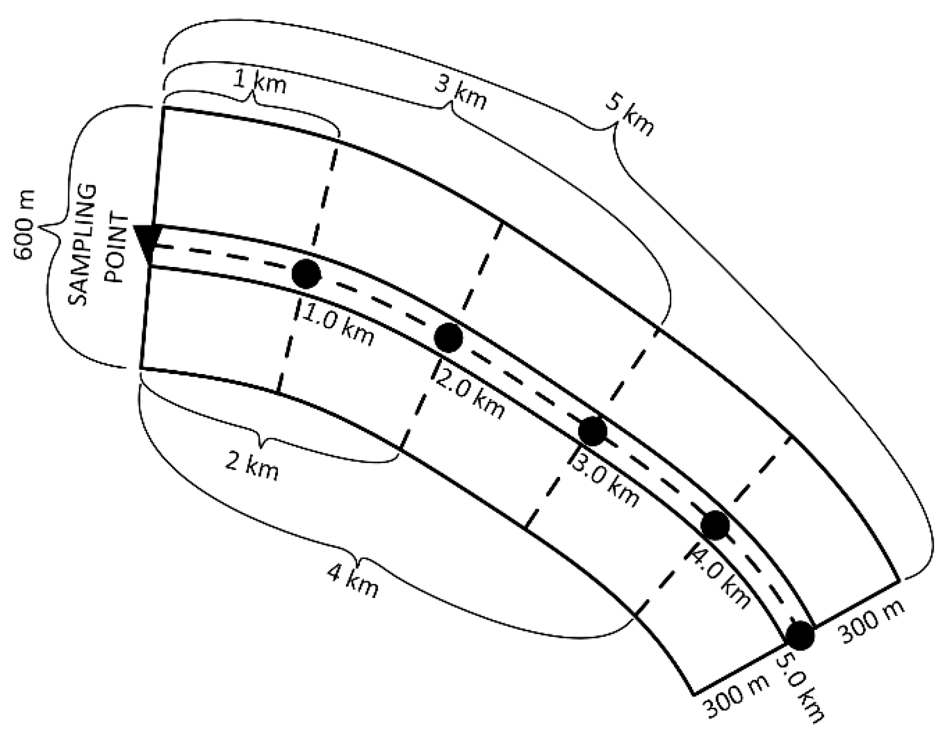
The Warta River of 808 km in length is the third longest river in Poland. Its catchment area is 54.5.103 km2, which makes about 17.4% of the area of Poland. The river flows in the western part of Poland and is the right tributary of the river Odra. The main tributaries of the Warta River are: Ner, Prosna, Obra, and Noteć (Figure 1). The source of the Warta River is at the altitude of about 380 m a.s.l., while its mouth is at 12 m a.s.l. The parent rocks of the soil in the river catchment area are postglacial formations. The near-surface layer is dominated with sand and clay formations. The dominant form of land use in the catchment area of the Warta River is agriculture (arable land), covering about 60% of the whole area. The total annual precipitation in the area varies from over 650 mm in the upper course (the Krakowsko-Częstochowska Upland) to nearly 500 mm in the middle course (e.g., catchment area of the upper course of the river Noteć), for the sake of comparison the mean annual precipitation for Poland is 600 mm.

2.2. Materials

The analysis was made on the basis of the measurements of the concentrations of the metals: Cr, Ni, Cu, Zn, Cd, and Pb in the bottom sediments of the Warta River, performed within the program of State Monitoring of the Natural Environment from the period of 2016–2017. Samples of the river bottom sediments were collected in 2016 and 2017 at 24 sample collection stations localized along the course of the Warta River (Figure 1). Sample collection stations were located at the borders of the catchment area, at the mouths of tributaries and below large cities or towns where industrial plants are located. Chemical analysis was performed for a 5 cm thick surface layer of the bottom sediment collected at, from 4 to 5 sites over a section of 50 m for each of the 24 sample collection stations. The samples were mixed and subjected to chemical analysis. Measurements were made by the inductively coupled plasma atomic emission spectroscopy (ICP–OES) according to PN-EN ISO 11885:2009 PB/I/13/D:04.2013.
The boundaries of the Warta River basin area were delimited on the basis of the Raster Hydrographical Map of Poland (MPHP) developed by the Section of Hydrography and Morphology of Riverbeds of the Institute of Meteorology and Water Management (IMGW). The map shows a complete hydrography of Poland in vector format at a scale of 1:50000, in the PUWG-92 coordinate system. The type of landscape sculpture was characterized on the basis of the Digital Terrain Model (DTM) of the mesh size of at least 100 m, provided by the Head Office of Geodesy and Cartography (GUGiK). The structure of land use over the river basin area was characterized on the basis of the digital database Corine Land Cover (CLC) obtained from the Chief Inspectorate of Environmental Protection.

2.3. Methods

Analysis of the content of heavy metals in the Warta River bottom sediments was performed in four stages. At first, a general characterization of the contents of heavy metals in the bottom sediments in 2016 and 2017 was made using the basic tools of statistical analysis. The second stage was devoted to assessment of contamination of the bottom sediments with heavy metals based on the calculation of Geoaccumulation Index (Igeo), Enrichment Factor (EF), Pollution Load Index (PLI), and Metal Pollution Index (MPI). At the third stage analysis of the possible hazardous effects of the heavy metals present in the river bottom sediments on the water flora and fauna was made using the procedure proposed by MacDonald et al. [37] based on the Threshold Effect Concentration (TEC), Probable Effect Concentration (PEC), and Midpoint Effect Concentration (MEC). Another parameter taken into account was the Toxic Risk Index (TRI), which permitted identification of the sample collection stations running the highest risk of toxic effect of heavy metals on water organisms. At the last stage, the multidimensional statistical methods were used to identify the river sections of similar contents of heavy metals in bottom sediments and to expose potential sources of contamination. Moreover, the content of heavy metals in bottom sediments was analyzed in relation to the hydrological conditions in the years 2016 and 2017, as well as the structure of land use in the land zone adjacent to the river, above the sampling site. It was expected to show if the content of heavy metals was increasing down the river.

2.3.1. General Characterization of the Content of Heavy Metals in the Warta River Bottom Sediments

To characterize the contents of the metals Cr, Ni, Cu, Zn, Cd, and Pb in the Warta River bottom sediments, the mean concentrations of the metals, their minimum and maximum values and median were calculated. The calculations were performed for 2016 and 2017 separately and jointly for the two years. For each metal, the percentiles were found (1%, 5%, 10%, 25%, 50%, 75%, 90%, 95%, and 99%). The data on the concentrations of Cr, Ni, Cu, Zn, Cd, and Pb were analyzed to establish the type of the values distribution, the presence of divergent results and the character of their variation. The distributions of Cr, Ni, Cu, Zn, Cd, and Pb concentration were characterized by performing one-sample Kolmogorov–Smirnov test (K–S). The divergent results in the analyzed data set were detected with the Grubbs–Beck (G–B) test. As the distributions of concentrations of all heavy metals considered differed from the normal distribution, in further analysis the nonparametric methods were applied. The Kruskal–Wallis (K–W) test and Dunn’s test, as a post-hoc procedure, were used to find out the possible differences in the median values of concentrations of particular metals between 2016 and 2017. The variations in the concentrations of Cr, Ni, Cu, Zn, Cd, and Pb in the years 2016 and 2017 were characterized on the basis of the range, interquartile range (IQR), median absolute deviation (MAD), and quartile coefficient of dispersion (QCD). The correlations between the concentrations of particular heavy metals in the bottom sediments were checked using the Spearman’s rank correlation coefficient. The Grubbs–Beck (G–B) test, Kruskal–Wallis (K–W), and Dunn’s test, Kolmogorov–Smirnov test (K–S) and Spearman’s correlation analysis were carried out using the STATISTICA software version 13.1 (Statistica).

2.3.2. Geoaccumulation Index

The Geoaccumulation Index (Igeo) was first developed by Muller [35] and is used to assess different pollution levels in bottom sediments and soils. The value of Igeo was calculated from the following, Equation (1):
Igeo = log2[Ci/1.5Bi],
where Ci is the concentration of each heavy metal (HM) in the sediment (mg·kg-1) and Bi is reference geochemical background value of each HM.
The following geochemical background values were adopted in this study: Cd—0.5 mg·kg−1, Cu—6 mg·kg−1, Cr—5 mg·kg−1, Fe—10000 mg·kg−1, Ni—5 mg·kg−1, Pb—10 mg·kg−1 and Zn—48 mg·kg−1 [38]. The factor 1.5 is used for correction of the possible variability of the background data due to lithological conditions. On the basis of the Igeo value, the level of pollution of the bottom sediments can be classified into six different classes (Table 1) [39].

2.3.3. Enrichment Factor

Calculation of the Enrichment Factor (EF) allows differentiation of the sources of metals, which can be natural or anthropogenic. EF is mostly used for quantification of the human impact on the concentration of each HM in sediments [40]. The Enrichment Factor describes the stabilization of sediments relative to reference elements, e.g., aluminum (Al), iron (Fe), manganese (Mn), scandium (Sc), or titanium (Ti) [26,41]. In this study, anthropogenic metal enrichment was measured by using iron (Fe) as a reference element. The EF values were calculated as Equation (2):
EFi = (Ci/CFe) / (Bi/BFe),
where Ci is the concentration of each HM in the sediment (mg·kg−1), CFe is the concentration of iron (Fe), Bi is the reference geochemical background value of each HM, BFe is the reference geochemical background value of iron (Fe). On the basis of the obtained EF values, bottom sediments can be classified into different classes presented in Table 2 [42].

2.3.4. Pollution Load Index

The Pollution Load Index (PLI) was originally developed by Tommilson et al. [36] to assess the extent of pollution status of the summarized heavy metals (HMs) in bottom sediments. The PLI is calculated as follows Equation (3):
PLI   =   ( CF i 1 ×   CF i 2   ×     ×   CF in ) 1 n ,
where n is the number of heavy metals and CF is a contamination factor defined for each studied heavy metal, which is one of the most recognized and effective tools in monitoring the heavy metal concentrations. The value of CF was calculated from the following Equation (4) [43]:
CFi = Ci/Bi,
where Ci is the concentration of each HM in the sediment (mg·kg-1) and Bi is the reference geochemical background value of each HM.
On the basis of the PLI, the Warta River bottom sediments can be classified into two classes: no pollution (PLI < 1) or pollution (PLI ≥ 1).

2.3.5. Metal Pollution Index

The Metal Pollution Index (MPI) is a presentation of all metal concentrations in sediments as a single value, overcoming the difficulties with application and understanding statistical analysis [44]. To compare the total content of all heavy metals at different sample collection stations, the MPI was calculated from Equation (5):
MPI   =   ( C i 1 ×   C i 2   ×     ×   C in ) 1 n ,
where Ci is the concentration of each HM in the sediment (mg·kg-1) and n is the number of heavy metals considered.

2.3.6. Ecological Risk Assessment

In order to assess the ecological risk of the impact of heavy metals on aquatic organisms the ecotoxicological criteria were applied. Assessment of the potential toxic effects of heavy metals accumulated in bottom sediments was made on the basis of TEC, MEC and PEC values [37]. The Threshold Effect Concentration (TEC) value is defined as the limit below which no harmful effects on aquatic organisms are expected, the Probable Effect Concentration (PEC) marks the limit above which a toxic effect on aquatic organisms can be expected. The Midpoint Effects Concentrations (MEC) is the mean of TEC and PEC limits. On the basis of the method proposed by MacDonald et al. [37], four levels of bottom sediment pollution and their impact on organisms have been distinguished (Table 3). According to the adopted methodology, the sediments classified as level I, II, III (≤PEC) may cause sporadic harmful effects on organisms, while the sediments at level IV (>PEC) often have harmful effect on living organisms. It is assumed that the sediments are classified as harmful to living organisms when PEC calculated for at least one analyzed heavy metal in the sediments exceeds the limit value.

2.3.7. Toxic Risk Index

Toxic Risk Index (TRI) was introduced by Zhang et al. [45] to assess potential integrated toxic risk caused by heavy metals to aquatic organisms. The TRI values calculated on the basis of the threshold (TEC) and probable (PEC) effect concentrations of heavy metals are presented in Table 2. The TEC and PEC values have been successfully used to assess ecological risk in many previous studies concerning rivers, lakes and reservoirs sediments [23,45,46]. The Toxic Risk Index is calculated according to the following Equation (6):
TRI   =   i = 1 n TRI i =   { [ ( C i / TEC i ) 2 + ( C i / PEC i ) 2 ] / 2 } 1 2 ,
where n is the number of HMs, Ci is the concentration of each HM in the sediment (mg·kg−1), TECi is the threshold effect concentration of each HM, PECi is the probable effect concentration of each HM, and TRIi is the toxic risk index of each HM. The toxic risks are classified into five categories based on the obtained TRI values [47] (Table 4).

2.3.8. Analysis of Spatial Variability of the Heavy Metal Content in the Warta River Bottom Sediments

Cluster analysis (CA) was applied to distinguish the groups of the sample collection stations at which the bottom sediments samples revealed similar contents of heavy metals. The grouping was performed by the Ward method assuming the square of Euclidean distance as a measure of similarity. The division of sample collection stations into groups and subgroups was made assuming the limits of Dlink.Dlnik.max.100% at 66% and 25% [48]. For the groups and subgroups the mean heavy metal concentrations and median were calculated. The differences in heavy metal concentrations between the groups and subgroups were analyzed by the nonparametric Kruskal–Wallis (K–W) test and Dunn’s tests as post hoc procedures. The cluster analysis (CA) was carried out using STATISTICA software (version 13.1, StatSoft, Kraków, Poland).
The types of land use were established for the zone adjacent to the river of 600 m in width. Taking into account great differences in spatial concentration of heavy metals, independent of the km of the river course, the land use character was analyzed separately at the distances of 1, 2, 3, 4, and 5 km from the sample collection station (Figure 2). The structure of land cover in the zone adjacent to the river was analyzed using the ArcGIS software and Buffer function.

2.3.9. Linear Interpolation

Point representation of the data on the contamination with heavy metals does not permit presentation of the changes taking place along the river course in a continuous way. However, on the basis of the point data a linear interpolation was performed to make a graphic presentation of the distribution of heavy metal contamination in the form of raster graphics of pixel resolution of 100 m. The linear interpolation can be described by Equation (7):
Ci = ((Cx − Cy) /pxy) · pxi + Cx,
where Ci is the concentration of each HM in the sediment (mg·kg−1) in the cell, Cx—the concentration of each HM in the sediment (mg·kg−1) at the point of measurement below a reference localization along the river course, pxy—the number of pixels of a certain spatial resolution between the points of measurements, pxi—the number of pixels between the point of measurement below along the river course and the reference point (Figure 3). The linear interpolation was performed in the ArcGIS software (10.7 version, ESRI, Redlands, California, CA, USA).

3. Results

3.1. General Characterization of Heavy Metal Concentrations

The concentrations of Cd, Cr, Cu, Ni, Pb, and Zn in the samples of the Warta River bottom sediments measured in 2016 and 2017 at particular sample collection stations are presented in Table 5, with reference to the values of TEC, MEC, and PEC. The concentrations of individual metals in the river bottom sediments varied in the following ranges: Cd: 0.03–14.50 mg·kg−1, Cr: 0.78–193.0 mg·kg−1, Cu: 0.40–116.0 mg·kg−1, Ni: 0.56–36.7 mg·kg−1, Pb: 1.0–144.0 mg·kg−1 and Zn: 0.50–519.0 mg·kg−1 (Table 5 and Table 6). Analysis of the data set with the Grubbs–Beck (G–B) test revealed a number of deviating results. In 2016 the deviating observations included the concentrations of Cd at site numbers 19, 20, and 23, and the concentrations of Cu and Pb at site 23. In 2017, the deviating observations were the concentration of Cr at site 1 and that of Pb at sites 1 and 24. Analysis of the concentrations of Cd, Cr, Cu, Ni, Pb, and Zn proved that they showed mostly a logarithmic-normal distribution, only the concentrations of Ni in 2016 showed a normal distribution.
On the basis of the measured concentrations of individual metals, their minimum, maximum mean values and median were calculated. Moreover, for each metal considered, the percentile values were found (Table 6). The calculations were made separately for 2016 and 2017 as well as for the two years together. The mean concentrations of heavy metals in the Warta River bottom sediments in 2016 and 2017 can be ordered as Zn > Cr > Pb > Cu > Ni > Cd and Zn > Pb > Cr > Cu > Ni > Cd, respectively. The mean concentrations of all heavy metals considered were higher in 2016 than in 2017. Analysis of the differences between the medians of heavy metal concentrations in the bottom sediments in 2016 and 2017 performed by the nonparametric Kruskal–Wallis test proved that the differences were statistically significant for Cr, Ni, and Pb at the level of 0.05, while for Zn – at the level of 0.10. For Cd and Cu, the differences were statistically insignificant.
In 2016 the concentrations of Cr showed the highest variation, while in 2017—the concentrations of Pb. When considering the two years together, the highest variations were noted for the concentrations of Cd and Zn, while the lowest was for Ni. The variations of Cd, Cr, Cu, Ni, Pb, and Zn concentrations in 2016 and 2017 are presented in the form of violin plots (Figure 4), which clearly reveals the considerable variation of the concentrations of the analyzed metals as well as the fact that in 2016 the heavy metal concentrations showed greater variation than in 2017. Moreover, the mean concentrations of individual heavy metals (marked in Figure 4 as a square) were higher than the corresponding medians (marked as a cross). These results confirm the earlier results proving the right skewed distributions of Cd, Cr, Cu, Ni, Pb, and Zn in the Warta River bottom sediments. The exceptions are the concentrations of Ni in 2016, whose mean values and medians are close, indicating the normal distribution of concentrations.

3.2. Assessment of the Contamination of the Warta River Bottom Sediment

As follows from the calculated Igeo index values, the river bottom sediments were more contaminated in 2016 than in 2017. The highest contribution to the bottom sediments contamination with heavy metals in 2016 brought chromium; from among 24 samples, for six, the values of the Igeo index for Cr indicated heavy contamination, while for two samples—very heavy contamination. For two samples, the values of Igeo for Cd and Cu were in the range of heavy contamination, while for one sample Igeo for Pb indicated heavy contamination. At sample collection stations 14 and 24, the values of Igeo for all analyzed heavy metals were lower than zero, which points to no contamination of the bottom sediments, (Figure 5a). The highest level of contamination was detected for the bottom sediments at sample collection station 23, with Igeo for Cd, Cr, Cu, and Pb indicating heavy and very heavy contamination. In 2017, the general level of contamination with heavy metals was lower. Only at station 1, the Igeo value for Cr indicated very heavy contamination. For three samples collected at stations 19, 20, and 24 in the lower course of the Warta River, the Igeo values were higher than 2, which corresponds to moderate contamination of the bottom sediments (Figure 5b).
Analysis of the EF index data also revealed the heaviest contamination of the Warta River bottom sediments with Cr. In 2016, the values of EF calculated for Cr indicated higher than average contamination of the river bottom sediments (Figure 6).
The EF values calculated for Cd and Cu signaled the heavier contamination of the bottom sediments in the lower course of the Warta River. In 2016 for Ni the highest EF were obtained for the bottom sediments from the middle course of the river, while for Pb a similar level of contamination was noted along the whole course of the river. According to EF data, the poorest contamination of the bottom sediment was observed with Zn; only in the upper course of the river at a few sample collection stations elevated EF values were calculated (Figure 6). The elevated EF values found for almost all heavy metals considered along the whole river course imply that the contaminants come mainly from local point sources. In 2017, the EF values for Ni, Pb, and Zn were at a level indicating poor contamination of bottom sediments with these elements, however, the EF values for Cd, Cr, and Cu were higher, indicating above average contamination with these metals.
The calculated PLI values in the period 2016–2017 varied from 0.25 to 16.93. The mean PLI values calculated for the years 1016 and 2017 were 3.32 and 1.46, respectively. According to the PLI values analysis for the concentrations of all heavy metals jointly, the river bottom sediments were highly contaminated at 15 of the 24 sample collection stations in 2016 (Figure 7a), and at 11 of the 24 stations in 2017 (Figure 7b). At 17 sample collection stations, the PLI values decreased in 2017 relative to those in 2016, while only at seven stations did the PLI values increase in 2017. Particular attention should be given to the increase in the value of PLI at station 24 in 2017, relative to the value determined in 2016. In general, PLI values indicate the heaviest contamination of the bottom sediments in the low course of the river. In 2017, in the upper and middle course of the river, the data indicate the scattered character of contamination, suggesting its origin from point sources.
A similar picture of contamination of the Warta River bottom sediments with heavy metals emerges from the analysis of MPI values, pointing generally to a reduced level of contamination in 2017. The mean value of MPI in 2016 was 10.7 higher than that obtained in 2017. According to MPI analysis, in 2017 (MPI > 15) the highest contamination was noted at stations 1, 4, 18, 19, and 20. In 2016, the MPI values were higher than 15 at 11 of the 24 stations: 1, 4, 10, 12, 14, 15, 17, 19, 20, 21, 22, and 23 (Figure 8).

3.3. Toxic Effect of Heavy Metals

Analysis of the potential effect of heavy metals accumulated in the Warta River bottom sediments on aquatic organisms was performed according to the procedure proposed by MacDonald et al. [37]. It showed that in 2016 the PEC limits were exceeded at two sample collection stations: station 1 for Cr and station 23 for Cd, Cr, Pb, and Zn. In the vicinity of these stations, a harmful effect on living aquatic organisms is predicted (Figure 9). In 10 of the 24 stations, numbers 5, 6, 7, 8, 9, 11, 13, 16, 18, and 24, the concentrations of all heavy metals considered were lower than the TEC limit, which points to no harmful effect related to the presence of these elements in the river bottom sediments. At the other stations, the content of heavy metals in the river bottom sediments indicates sporadic toxic effect on aquatic organisms, at seven stations the heavy metal concentrations were above the TEC limit but below the MEC limit, while at five stations they were below the MEC limit. In 2017, only at station no. 1, the concentration of Cr was higher than the PEC limit, whereas at 15 stations, the concentrations of Cd, Cr, Cu, Ni, Pb, and Zn were lower than the TEC limit. At five sample collection stations, the river bottom sediments were contaminated with heavy metals at level II, according to the classification introduced by MacDonald et al. [37], while at three stations—at level III, which implied sporadic toxic effect on aquatic organisms. In general, the highest toxic threat to aquatic life had the high concentration of Cr and at some sites the concentrations of Cd, Pb, and Zn.
The values of TRI in 2016 varied from 0.37 to 23.77, with the mean value of 4.60. In 2017, TRI varied from 0.37 to 8.06, with the mean value of 2.04. Assessment of the potential toxic effect of heavy metals accumulated in the Warta River bottom sediments in 2016 indicated a small effect on aquatic life at the sample collection stations 1, 4, 14, 17, and 19. According to TRI, only at stations 20 and 23 a possible moderate and very strong effects, respectively, on aquatic organisms could occur (Figure 10a). In 2017, only at two stations, 1 and 20, were the values of TRI 8.06 and 6.42—so high enough to indicate a possible small toxic effect on aquatic life (Figure 10b).

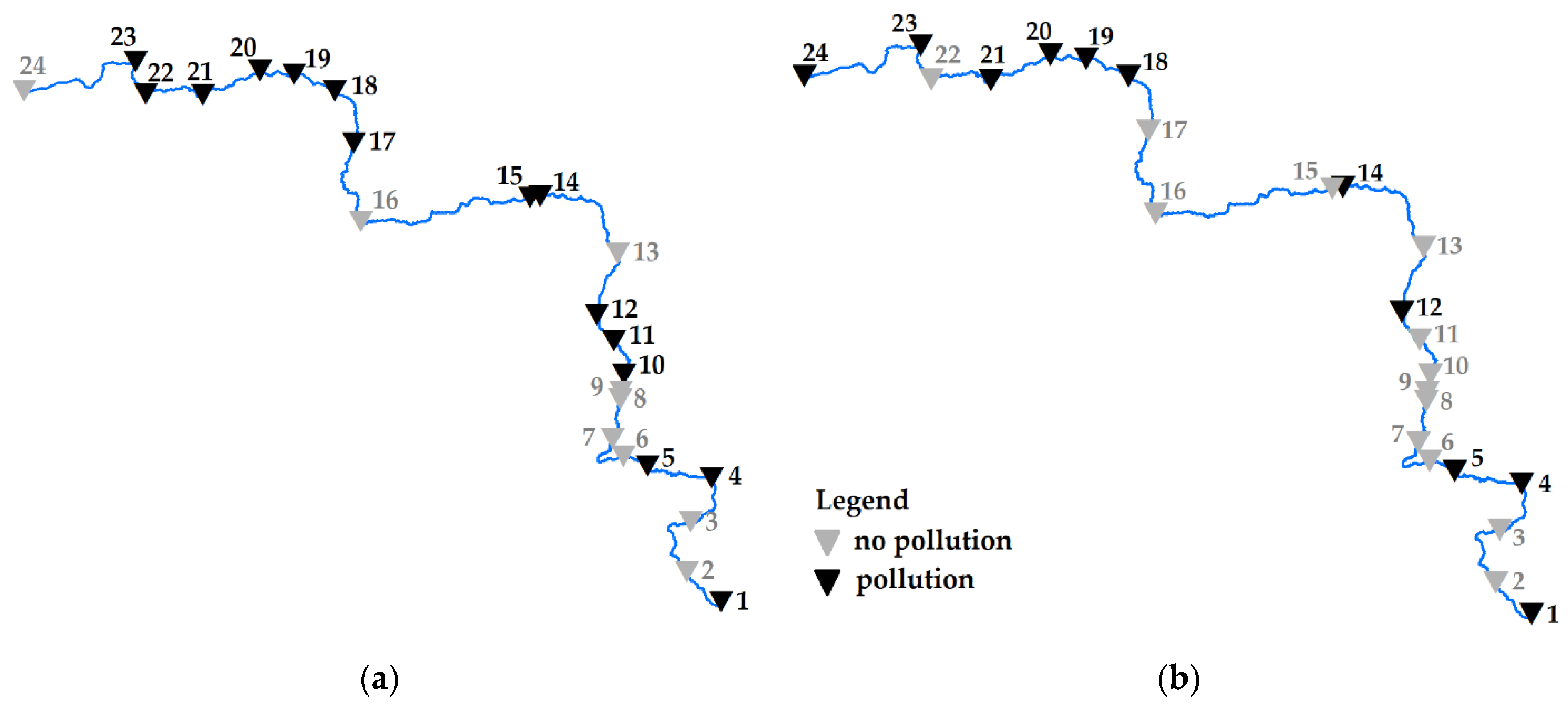
3.4. Spatial Analysis of Contamination of the Warta River Bottom Sediments with Heavy Metals

Cluster analysis was performed separately for the data for 2016 and 2017 (Figure 11a,b). The cluster analysis of the data from 2016 revealed two groups of stations at which the bottom sediment samples were characterized by similar concentrations of Cd, Cr, Cu, Pb, Ni, and Zn. Group 1 included 19 sample collection stations; the bottom sediment samples collected at them showed lower concentrations of Cd, Cr, Cu, Pb, Ni, and Zn than the samples collected at group 2 of stations. The differences between the medians of concentrations of Cd, Cr, Cu, Pb, Ni, and Zn calculated for groups 1 and 2 were statistically significant at the level of 0.05. The stations from group 1 were subdivided into two subgroups 1–1 and 1–2. The samples collected at the stations 1–1 were characterized by higher concentrations of all heavy metals considered than those collected at the stations 1–2. The differences were statistically significant at the level of 0.05. Group 2 included only five stations, of which four were localized in the low course of the Warta River, below the city of Poznań, the largest city on the river. On the basis of the data for 2017, the sample collection stations were also divided into two groups. Group 1 included seven stations, at which the samples of bottom sediments contained higher concentrations of all heavy metals considered than those collected at the stations from group 2. The differences were statistically significant at the level of 0.05. In 2017, the stations of group 1 included four stations, numbers 4, 19, 20, and 23, classified to group 2 in 2016. Moreover, three stations (no. 1, 18, and 24) were classified as those at which the bottom sediment samples showed the strongest contamination with the heavy metals studied. Similarly as in 2016, the stations at which the bottom sediment samples contain the greatest amounts of heavy metals were in the low course of the river, except stations 1 and 4, at which probably the effect of local anthropogenic sources of contamination was reflected. It should be mentioned that the samples collected at the stations from group 2 were characterized by greater variation of the heavy metals concentrations than those collected at the stations from group 1; however, the highest concentrations of heavy metals were found in the samples collected at stations 1 and 24.

3.5. Linear Interpolation

The main limitation of point measurements is the lack of possibility of presentation of changes in the heavy metals concentrations over the whole length of the river. On the basis of the concentrations determined at the stations, a linear interpolation was performed to obtain a graphical presentation of the contamination with heavy metals along the whole course of the river. Figure 12 presents the variation in the concentration of lead (Pb) along the river section between stations 22 and 24. Considering the results of the interpolation over this section it is apparent that the concentrations of lead in 2016 and 2017 were significantly different along the whole section, which implies that their negative effects can be significant not only near the sample collection stations, but also along the sections not subjected to monitoring. Linear interpolation of the data along the course of the river reveals important information both for identification of new sources of contamination and for making decisions on activities aimed at limitation of a given type contamination on the environment.

4. Discussion

According to the hitherto studies, the content of heavy metals in river bottom sediments is related to the terrain relief of the catchment area, hydrological conditions and anthropogenic activity in the catchment area, including the type of land use. Analysis of the data from a two-year period of monitoring the content of heavy metals (Cd, Cu, Ni, Zn, Fe, Pb, Cr, and Mn) in the mouths of the rivers revealed no seasonal changes and no relations to tides. The observed high content of heavy metals in the form of particles was probably a result of anthropogenic pressure [49]. Zhou et al. [50] determined the content of main and trace elements in bottom sediments of 26 large rivers in south China and on the basis of EF data analysis they concluded that high concentrations of As, Cd, Hg, Mn, Mo, Pb, and Zn in the majority of the rivers studied were strongly related to the natural factors, in particular to geological conditions. Le Gall et al. [51] analyzed the contamination of bottom sediments of the river Seine on the basis of determination of stable isotopes of lead and EF index. Their conclusion was that the contamination of the river bottom sediments below Paris was mainly caused by point influx from urbanized areas [51]. According to the results presented in our paper, the concentrations of some heavy metals in the Warta River bottom sediments show high variation over the period of the two years studied, 2016 and 2017. This character of results collected in two subsequent years may indicate a significant effect of point sources of contamination from urbanized areas on the heavy metal contents as in such a short period of time the type of land use was unchanged (Figure 13).
The results presented in this paper corroborate the conclusions drawn by Li et al. [52], who have identified the industrial activities as the largest contributor (48.0%) of heavy metals to the river–lake sediments, followed by the agricultural activities (27.3%) and mix sources (24.7%). Zeng et al. [46] have shown that heavy metal concentrations in the central city in a given area were generally higher than those in other areas. Heavy metals in sediments pose a considerable ecological risk. The main contributors to the contamination with heavy metals were Hg and Cd whose presence posed the highest potential ecological risk in the central city. According to Custodio et al. [53], the rivers of the Mantaro River watershed are exposed to contamination by heavy metals and metalloids from natural and anthropogenic sources; among the latter, the mining metallurgical industry, agricultural activity, and manufacturing industry are the main sources. One of the key variables affecting the heavy metals release from sediments are also hydrometeorological conditions [54]. River fluvial process depends on flow rate value, so flash floods and low flows also have impact on HMs concentration. According to Li et al. [54]. The flow rate significantly affected the release amount of Zn, Pb, and Cr, while it slightly affected the concentration of Cu and Cd.
Sojka et al. [23] have shown that the high values of Igeo, EF, PLI, and MPI in the samples collected at particular stations may indicate the anthropogenic origin of the heavy metal contamination and the influx of heavy metals from point sources. Bing et al. [47] have suggested that local anthropogenic activity increases the concentration of certain heavy metals in the river bottom sediments, in particular in the upper courses of the rivers. Saleem et al. [55] have reported a relatively high level of heavy metals at the sites close to large cities and towns. The results presented in this paper confirm the earlier observations indicating a significant effect of urbanized areas on the level of contamination with heavy metals in the river bottom sediments. This conclusion implies the necessity of looking for new solutions supporting monitoring and aimed at protection of water resources along the whole course of the river, e.g., with the use of GIS tools. New approach to classical interpolation method which that takes into account the curvature of the river was never presented regarding to HMs contamination. This interpolation method allows to receive accurate information on the status of the whole courses of the rivers not only at single sample points. The solution proposed in this paper permits analysis of the changes in the river bottom sediments along the whole course of the river, which is essential for identification of potential sources of contamination and for taking up actions aimed at limitation of the effect of such sources. The main limitation of the method proposed is the fact that it is based only on point measurements, disregarding a variable related to the land use, e.g., the effect of urbanized areas.

5. Conclusions

The above presented results and their analyses permit drawing the following conclusions:
  • As shown by the results of analysis of Igeo, EF, PLI, and MPI values, the level of contamination of the Warta River bottom sediments with heavy metals was higher in 2016 than in 2017.
  • According to the assessment of the potential toxic effects of heavy metals accumulated in bottom sediments made on the basis of TEC, MEC, PEC, and TRI, the ecological risk related to the presence of heavy metals in the river bottom sediments was much lower in 2017 than in 2016.
  • Cluster analysis permitted distinction of two groups of the sample collection stations at which bottom sediments showed similar chemical character. Changes in the classification of particular stations to particular groups indicated that the concentration of heavy metals in the Warta river bottom sediments is mainly related to the point sources of contamination in urbanized areas and connected with river fluvial process.
  • In view of the necessity of taking up measures aimed at protection of water resources, it is vital to find methods providing the possibly most accurate information on the status of the whole courses of the rivers not only at their certain points. The solution proposed in this paper permits analysis of the changes in the river bottom sediments along the whole course of the river, which is essential for identification of potential sources of contamination and for taking up actions aimed at limitation of the effect of such sources. The main drawback of the method proposed is the fact that it is based on point measurements, disregarding a variable related to the land use, e.g., the effect of urbanized areas.

Author Contributions

Conceptualization, J.J. and M.S.; methodology J.J. and M.S.; software, J.J. and M.S.; validation, J.J. and M.S.; investigation, J.J.; data curation, J.J., M.S., and M.F.; writing—original draft preparation, J.J. and M.S.; writing—review and editing, J.J; visualization, J.J., R.W.; project administration, J.J. All authors have read and agreed to the published version of the manuscript.

Funding

The publication was co-financed within the framework of the Ministry of Science and Higher Education programme as “Regional Initiative Excellence” in the years 2019–2022, Project No. 005/RID/2018/19.

Conflicts of Interest

The authors declare no conflict of interest.

References

  1. Dąbrowska, J.; Dąbek, P.B.; Lejcuś, I. A GIS based approach for the mitigation of surface runoff to a shallow lowland reservoir. Ecohydrol. Hydrobiol. 2018, 18, 420–430. [Google Scholar] [CrossRef]
  2. Dąbrowska, J.; Pawęska, K.; Dąbek, P.B.; Stodolak, R. The implications of economic development, climate change and European water policy on surface water quality threats. Acta Sci. Pol. Formatio Circumiectus 2017, 16, 111. [Google Scholar] [CrossRef] [Green Version]
  3. Tung, T.M.; Yaseen, Z.M. A survey on river water quality modelling using artificial intelligence models: 2000–2020. J. Hydrol. 2020, 585, 124670. [Google Scholar]
  4. Sojka, M.; Jaskuła, J.; Wicher-Dysarz, J. Assessment of Biogenic Compounds elution from the Główna River catchment in the Years 1996–2009. Annu. Set Environ. Prot. 2016, 18, 815–830. [Google Scholar]
  5. Kuriata-Potasznik, A.; Szymczyk, S.; Skwierawski, A. Influence of cascading river–lake systems on the dynamics of nutrient circulation in catchment areas. Water 2020, 12, 1144. [Google Scholar] [CrossRef] [Green Version]
  6. Sojka, M.; Siepak, M.; Jaskuła, J.; Wicher-Dysarz, J. Heavy metal transport in a river-reservoir system: A case study from central Poland. Pol. J. Environ. Stud. 2018, 27, 1725–1734. [Google Scholar] [CrossRef]
  7. Kuriata-Potasznik, A.; Szymczyk, S.; Skwierawski, A.; Glińska-Lewczuk, K.; Cymes, I. Heavy metal contamination in the surface layer of bottom sediments in a flow-through lake: A case study of Lake Symsar in Northern Poland. Water 2016, 8, 358. [Google Scholar] [CrossRef]
  8. Deng, Q.; Wei, Y.; Yin, J.; Chen, L.; Peng, C.; Wang, X.; Zhu, K. Ecological risk of human health posed by sediments in a karstic river basin with high longevity population. Environ. Pollut. 2020, 265, 114418. [Google Scholar] [CrossRef]
  9. Jaskuła, J.; Sojka, M.; Wicher-Dysarz, J. Analysis of the vegetation process in a two-stage reservoir on the basis of satellite imagery—a case study: Radzyny Reservoir on the Sama River. Annu. Set Environ. Prot. 2018, 20, 203–220. [Google Scholar]
  10. Jaskuła, J.; Sojka, M. Assessment of spectral indices for detection of vegetative overgrowth of reservoirs. Pol. J. Environ. Stud. 2019, 28, 4199–4211. [Google Scholar] [CrossRef]
  11. Dysarz, T.; Wicher-Dysarz, J.; Sojka, M.; Jaskuła, J. Analysis of extreme flow uncertainty impact on size of flood hazard zones for the Wronki gauge station in the Warta river. Acta Geophys. 2019, 67, 661–676. [Google Scholar] [CrossRef] [Green Version]
  12. Wicher-Dysarz, J.; Szałkiewicz, E.; Jaskuła, J.; Dysarz, T.; Rybacki, M. Possibilities of controlling the river outlets by weirs on the example of Noteć Bystra River. Sustainability 2020, 12, 2369. [Google Scholar] [CrossRef] [Green Version]
  13. Liu, M.; Chen, J.; Sun, X.; Hu, Z.; Fan, D. Accumulation and transformation of heavy metals in surface sediments from the Yangtze River estuary to the East China Sea shelf. Environ. Pollut. 2019, 245, 111–121. [Google Scholar] [CrossRef]
  14. Jain, C.K.; Sharma, M.K. Distribution of trace metals in the Hindon River system, India. J. Hydrol. 2001, 253, 81–90. [Google Scholar] [CrossRef]
  15. Nawrot, N.; Wojciechowska, E.; Rezania, S.; Walkusz-Miotk, J.; Pazdro, K. The effects of urban vehicle traffic on heavy metal contamination in road sweeping waste and bottom sediments of retention tanks. Sci. Total Environ. 2020, 749, 141511. [Google Scholar] [CrossRef]
  16. Mandeng, E.P.B.; Bidjeck, L.M.B.; Bessa, A.Z.E.; Ntomb, Y.D.; Wadjou, J.W.; Doumo, E.P.E.; Dieudonné, L.B. Contamination and risk assessment of heavy metals, and uranium of sediments in two watersheds in Abiete-Toko gold district, Southern Cameroon. Heliyon 2019, 5, e02591. [Google Scholar] [CrossRef] [Green Version]
  17. Sun, X.; Fan, D.; Liu, M.; Tian, Y.; Pang, Y.; Liao, H. Source identification, geochemical normalization and influence factors of heavy metals in Yangtze River Estuary sediment. Environ. Pollut. 2018, 241, 938–949. [Google Scholar] [CrossRef]
  18. Duodu, G.O.; Goonetilleke, A.; Ayoko, G.A. Comparison of pollution indices for the assessment of heavy metal in Brisbane River sediment. Environ. Pollut. 2016, 219, 1077–1091. [Google Scholar] [CrossRef]
  19. Stamatis, N.; Kamidis, N.; Pigada, P.; Sylaios, G.; Koutrakis, E. Quality Indicators and Possible Ecological Risks of Heavy Metals in the Sediments of three Semi-closed East Mediterranean Gulfs. Toxics 2019, 7, 30. [Google Scholar] [CrossRef] [Green Version]
  20. He, Z.; Li, F.; Dominech, S.; Wen, X.; Yang, S. Heavy metals of surface sediments in the Changjiang (Yangtze River) Estuary: Distribution, speciation and environmental risks. J. Geochem. Explor. 2019, 198, 18–28. [Google Scholar] [CrossRef]
  21. Brady, J.P.; Ayoko, G.A.; Martens, W.N.; Goonetilleke, A. Enrichment, distribution and sources of heavy metals in the sediments of Deception Bay, Queensland, Australia. Mar. Pollut. Bull. 2014, 81, 248–255. [Google Scholar] [CrossRef] [PubMed] [Green Version]
  22. Wu, Q.; Qi, J.; Xia, X. Long-term variations in sediment heavy metals of a reservoir with changing trophic states: Implications for the impact of climate change. Sci. Total Environ. 2017, 609, 242–250. [Google Scholar] [CrossRef]
  23. Sojka, M.; Jaskuła, J.; Siepak, M. Heavy metals in bottom sediments of reservoirs in the lowland area of western Poland: Concentrations, distribution, sources and ecological risk. Water 2019, 11, 56. [Google Scholar] [CrossRef] [Green Version]
  24. Doležalová Weissmannová, H.; Mihočová, S.; Chovanec, P.; Pavlovský, J. Potential ecological risk and human health risk assessment of heavy metal pollution in industrial affected soils by coal mining and metallurgy in Ostrava, Czech Republic. Int. J. Environ. Res. Public Health 2019, 16, 4495. [Google Scholar] [CrossRef] [PubMed] [Green Version]
  25. Gao, L.; Wang, Z.; Shan, J.; Chen, J.; Tang, C.; Yi, M.; Zhao, X. Distribution characteristics and sources of trace metals in sediment cores from a trans-boundary watercourse: An example from the Shima River, Pearl River Delta. Ecotox. Environ. Safe 2016, 134, 186–195. [Google Scholar] [CrossRef]
  26. Ahamad, M.I.; Song, J.; Sun, H.; Wang, X.; Mehmood, M.S.; Sajid, M.; Khan, A.J. Contamination level, ecological risk, and source identification of heavy metals in the hyporheic zone of the Weihe River, China. Int. J. Environ. Res. Public Health 2020, 17, 1070. [Google Scholar] [CrossRef] [Green Version]
  27. Malvandi, H. Preliminary evaluation of heavy metal contamination in the Zarrin-Gol River sediments, Iran. Mar. Pollut. Bull. 2017, 117, 547–553. [Google Scholar] [CrossRef]
  28. Dong, X.; Wang, C.; Li, H.; Wu, M.; Liao, S.; Zhang, D.; Pan, B. The sorption of heavy metals on thermally treated sediments with high organic matter content. Bioresour. Technol. 2014, 160, 123–128. [Google Scholar] [CrossRef]
  29. Cymes, I.; Glińska-Lewczuk, K.; Szymczyk, S.; Sidoruk, M.; Potasznik, A. Distribution and potential risk assessment of heavy metals and arsenic in sediments of a dam reservoir: A case study of the Łoje retention reservoir, NE Poland. J. Elementol. 2017, 22. [Google Scholar] [CrossRef]
  30. Nguyen, B.T.; Do, D.D.; Nguyen, T.X.; Nguyen, V.N.; Nguyen, D.T.P.; Nguyen, M.H.; Bach, Q.V. Seasonal, spatial variation, and pollution sources of heavy metals in the sediment of the Saigon River, Vietnam. Environ. Pollut. 2020, 256, 113412. [Google Scholar] [CrossRef]
  31. Lin, Q.; Liu, E.; Zhang, E.; Li, K.; Shen, J. Spatial distribution, contamination and ecological risk assessment of heavy metals in surface sediments of Erhai Lake, a large eutrophic plateau lake in southwest China. Catena 2016, 145, 193–203. [Google Scholar] [CrossRef]
  32. Bibi, M.H.; Ahmed, F.; Ishiga, H. Assessment of metal concentrations in lake sediments of southwest Japan based on sediment quality guidelines. Environ. Geol. 2007, 52, 625–639. [Google Scholar] [CrossRef]
  33. Noronha-D’Mello, C.A.; Nayak, G.N. Assessment of metal enrichment and their bioavailability in sediment and bioaccumulation by mangrove plant pneumatophores in a tropical (Zuari) estuary, west coast of India. Mar. Pollut. Bull. 2016, 110, 221–230. [Google Scholar] [CrossRef] [PubMed]
  34. Lee, A.S.; Huang, J.J.S.; Burr, G.; Kao, L.C.; Wei, K.Y.; Liou, S.Y.H. High resolution record of heavy metals from estuary sediments of Nankan River (Taiwan) assessed by rigorous multivariate statistical analysis. Quat. Int. 2019, 527, 44–51. [Google Scholar] [CrossRef]
  35. Muller, G. Index of geoaccumulation in sediments of the Rhine River. Geol. J. 1969, 2, 108–118. [Google Scholar]
  36. Tomlinson, D.L.; Wilson, J.G.; Harris, C.R.; Jeffrey, D.W. Problems in the assessment of heavy-metal levels in estuaries and the formation of a pollution index. Helgol. Mar. Res. 1980, 33, 566–575. [Google Scholar] [CrossRef] [Green Version]
  37. MacDonald, D.D.; Ingersoll, C.G.; Berger, T.A. Development and evaluation of consensus-based sediment quality guidelines for freshwater ecosystems. Arch. Environ. Contam. Toxicol. 2000, 39, 20–31. [Google Scholar] [CrossRef]
  38. Bojakowska, I.; Sokołowska, G. Geochemiczne klasy czystości osadów wodnych. Przegląd Geologiczny 1998, 46, 49–54. [Google Scholar]
  39. Sakan, S.M.; Đorđević, D.S.; Manojlović, D.D.; Predrag, P.S. Assessment of heavy metal pollutants accumulation in the Tisza river sediments. J. Environ. Manage. 2009, 90, 3382–3390. [Google Scholar] [CrossRef]
  40. Selvaraj, K.; Ram Mohan, V.; Szefer, P. Evaluation of metal contamination in coastal sediments of the Bay of Bengal, India: Geochemical and statistical approaches. Mar. Pollut. Bull. 2004, 49, 174–185. [Google Scholar] [CrossRef]
  41. Salati, S.; Moore, F. Assessment of heavy metal concentration in the Khoshk River water and sediment, Shiraz, Southwest Iran. Environ. Monit. Assess. 2010, 164, 677–689. [Google Scholar] [CrossRef] [PubMed]
  42. Al Rashdi, S.; Arabi, A.A.; Howari, F.M.; Siad, A. Distribution of heavy metals in the coastal area of Abu Dhabi in the United Arab Emirates. Mar. Pollut. Bull. 2015, 97, 494–498. [Google Scholar] [CrossRef] [PubMed]
  43. Martin, J.M.; Meybeck, M. Elemental mass-balance of material carried by major world rivers. Mar. Chem. 1979, 7, 173–206. [Google Scholar] [CrossRef]
  44. Singovszka, E.; Balintova, M.; Demcak, S.; Pavlikova, P. Metal pollution indices of bottom sediment and surface water affected by acid mine drainage. Metals 2017, 7, 284. [Google Scholar] [CrossRef]
  45. Zhang, G.; Bai, J.; Zhao, Q.; Lu, Q.; Jia, J.; Wen, X. Heavy metals in wetland soils along a wetland-forming chronosequence in the Yellow River Delta of China: Levels, sources and toxic risks. Ecol. Indic. 2016, 69, 331–339. [Google Scholar] [CrossRef] [Green Version]
  46. Zeng, Y.; Bi, C.; Jia, J.; Deng, L.; Chen, Z. Impact of intensive land use on heavy metal concentrations and ecological risks in an urbanized river network of Shanghai. Ecol. Indic. 2020, 116, 106501. [Google Scholar] [CrossRef]
  47. Bing, H.; Wu, Y.; Zhou, J.; Sun, H.; Wang, X.; Zhu, H. Spatial variation of heavy metal contamination in the riparian sediments after two-year flow regulation in the Three Gorges Reservoir, China. Sci. Total Environ. 2019, 649, 1004–1016. [Google Scholar] [CrossRef]
  48. Ptak, M.; Sojka, M.; Choiński, A.; Nowak, B. Effect of environmental conditions and morphometric parameters on surface water temperature in Polish lakes. Water 2018, 10, 580. [Google Scholar] [CrossRef] [Green Version]
  49. Beltrame, M.O.; De Marco, S.G.; Marcovecchio, J.E. Dissolved and particulate heavy metals distribution in coastal lagoons. A case study from Mar Chiquita Lagoon, Argentina. Estuar. Coast. Shelf Sci. 2009, 85, 45–56. [Google Scholar] [CrossRef]
  50. Zhou, G.; Sun, B.; Zeng, D.; Wei, H.; Liu, Z.; Zhang, B. Vertical distribution of trace elements in the sediment cores from major rivers in east China and its implication on geochemical background and anthropogenic effects. J. Geochem. Explor. 2014, 139, 53–67. [Google Scholar] [CrossRef]
  51. Le Gall, M.; Ayrault, S.; Evrard, O.; Laceby, J.P.; Gateuille, D.; Lefevre, I.; Mouchel, J.M.; Meybeck, M. Investigating the metal contamination of sediment transported by the 2016 Seine River flood (Paris, France). Environ. Pollut. 2018, 240, 125–139. [Google Scholar] [CrossRef] [PubMed]
  52. Li, Y.; Chen, H.; Teng, Y. Source apportionment and source-oriented risk assessment of heavy metals in the sediments of an urban river-lake system. Sci. Total Environ. 2020, 737, 140310. [Google Scholar] [CrossRef] [PubMed]
  53. Custodio, M.; Cuadrado, W.; Peñaloza, R.; Montalvo, R.; Ochoa, S.; Quispe, J. Human risk from exposure to heavy metals and arsenic in water from rivers with mining influence in the Central Andes of Peru. Water 2020, 12, 1946. [Google Scholar] [CrossRef]
  54. Li, H.; Shi, A.; Li, M.; Zhang, X. Effect of pH, temperature, dissolved oxygen, and flow rate of overlying water on heavy metals release from storm sewer sediments. J. Chem. 2013, 2013, 1–11. [Google Scholar] [CrossRef]
  55. Saleem, M.; Iqbal, J.; Akhter, G.; Shah, M.H. Fractionation, bioavailability, contamination and environmental risk of heavy metals in the sediments from a freshwater reservoir, Pakistan. J. Geochem. Explor. 2018, 184, 199–208. [Google Scholar] [CrossRef]
Figure 1. Study site location.
Minerals 11 00327 g001
Figure 2. Scheme of land cover analysis.
Minerals 11 00327 g002
Figure 3. Scheme of linear interpolation developed in this study.
Minerals 11 00327 g003
Figure 4. Variation of the concentrations of (a) Cd, (b) Cr, (c) Cu, (d) Ni, (e) Pb, and (f) Zn in the Warta River bottom sediments in 2016 and 2017.
Minerals 11 00327 g004aMinerals 11 00327 g004b
Figure 5. Geoaccumulation Index (Igeo) in bottom sediments of the Warta River in 2016 (a) and 2017 (b).
Minerals 11 00327 g005
Figure 6. Enrichment Factor (EF) in bottom sediments of Warta River in 2016 and 2017.
Minerals 11 00327 g006
Figure 7. Classes of Pollution Load Index (PLI) in bottom sediments of the Warta River in 2016 (a) and 2017 (b).
Minerals 11 00327 g007
Figure 8. Comparison of Metal Pollution Index (MPI) in bottom sediments of Warta River in 2016 and 2017.
Minerals 11 00327 g008
Figure 9. Ecotoxicological criteria for assessing the lakes quality using TEC, MEC, and PEC values in bottom sediments of Warta River in 2016 and 2017.
Minerals 11 00327 g009
Figure 10. Toxic Risk Index (TRI) in bottom sediments of Warta River in 2016 (a) and 2017 (b).
Minerals 11 00327 g010
Figure 11. Division of sample collection stations into groups as a result of cluster analysis: in 2016 (a) and 2017 (b).
Minerals 11 00327 g011
Figure 12. Linear interpolation of Pb concentration between sample collection stations 22–24.
Minerals 11 00327 g012
Figure 13. Land cover analysis.
Minerals 11 00327 g013
Table 1. Geoaccumulation Index (Igeo) classification.
ClassValueSediment Pollution
0Igeo ≤ 0no enrichment
10 < Igeo ≤ 1minor enrichment
21 < Igeo ≤ 2moderate enrichment
32 < Igeo ≤ 3moderately severe enrichment
43 < Igeo ≤ 4severe enrichment
54 < Igeo ≤ 5very severe enrichment
65 < Igeo extremely severe enrichment
Table 2. Enrichment Factor (EF) classification.
ClassValueSediment Pollution
0       EF ≤ 1no enrichment
11 < EF ≤ 3minor enrichment
23 < EF ≤ 5moderate enrichment
35 < EF ≤ 10moderately severe enrichment
410 < EF ≤ 25severe enrichment
525 < EF ≤ 50very severe enrichment
650 < EFextremely severe enrichment
Table 3. Ecotoxicological criteria for assessing the quality of bottom sediments using the Threshold Effect Concentration (TEC), Midpoint Effect Concentration (MEC), and Probable Effect Concentration (PEC) values (mg·kg−1).
HMsLevel I
(≤ TEC)
Level II
(>TEC ≤ MEC)
Level III
(>MEC ≤ PEC)
Level IV
(>PEC)
Cd≤0.990.99–3.03.0–5.0>5.0
Cr≤4343–76.576.5–110 >110
Cu≤3232–9191–150>150
Ni≤2323–3636–49>49
Pb≤3636–8383–130>130
Zn≤120120–290290–460>460
Table 4. Toxic Risk Index (TRI) classification.
ClassValueToxic Risk
0     TRI ≤ 5no toxic risk
15 < TRI ≤ 10low
210 < TRI ≤ 15moderate
315 < TRI ≤ 20considerable
420 < TRIvery high
Table 5. Concentrations of heavy metals in the bottom sediments of Warta River (mg·kg−1) in 2016 and 2017 on the background of ecotoxicological criteria.
No.HMs
CdCrCuNiPbZn
201620172016201720162017201620172016201720162017
10.370.53193.00152.00 *23.2036.9822.2016.8027.00106.00 *168.00234.00
20.520.474.320.780.402.932.840.7712.005.99200.00168.50
30.130.0317.406.260.406.1210.305.9916.006.32132.0055.79
42.621.0441.4025.0539.1020.0728.6016.6669.0041.66440.00207.50
50.050.3137.004.126.5014.3013.103.2115.0027.9058.9031.20
60.050.1712.606.571.165.1215.9010.116.006.2673.1048.48
70.050.125.754.200.914.4912.402.471.003.3211.1013.52
80.050.1939.307.333.097.4814.406.2316.007.720.5029.84
90.050.0319.603.464.551.429.963.7612.001.9140.8024.31
100.050.0352.202.908.282.4021.902.4734.002.1364.6019.62
110.210.0639.403.467.743.7918.602.5827.004.3522.8021.11
120.610.3164.5013.7911.206.9119.706.3643.0010.3084.2055.35
130.050.5433.301.412.547.3013.801.0915.002.940.506.09
142.160.4486.3015.2323.808.6916.603.8827.009.12170.0046.45
150.960.2963.107.1121.003.5218.401.9426.006.90153.0025.67
160.051.156.603.170.4011.921.481.652.003.9019.809.05
171.560.05100.004.6883.804.8220.201.9385.005.95327.0014.44
180.472.0027.4024.4010.2024.348.927.4917.0021.3878.6097.10
194.22 *3.2369.6035.8952.6021.7723.206.8645.0021.39296.0095.61
206.46 *3.5281.3040.2658.3039.0021.6016.6052.0031.81283.00173.50
210.710.6756.9010.6612.3010.1724.904.5834.0010.1874.7038.67
221.700.1227.002.1238.209.607.360.5619.004.1288.9019.02
2314.50 *1.17184.00 *21.33116.0016.1136.706.61144.00 *16.22519.0067.95
240.050.123.206.569.0013.551.301.9110.0090.47*11.3095.45
*-deviating values, Ecotoxicological criteria for assessment of the lakes quality using TEC, MEC, and PEC values: X—level 1, X—level 2, X—level 3, X—level 4.
Table 6. The characteristic concentrations of heavy metals (mg.kg−1) in the Warta River bottom sediments in 2016 and 2017.
Period201620172016/2017
HMsCdCrCuNiPbZnCdCrCuNiPbZnCdCrCuNiPbZn
Minimum0.053.200.401.301.000.500.030.781.420.561.916.090.030.780.400.561.000.50
Mean1.5752.722.316.031.41380.6916.811.85.5218.766.61.1334.717.010.825.0102
Maximum14.519311636.71445193.515239.016.810623414.519311636.7144519
Percentile1%0.053.200.401.301.000.500.030.781.420.561.916.090.030.780.400.561.000.50
5%0.054.320.401.482.000.500.031.412.400.772.139.050.032.120.401.092.006.09
10%0.055.750.402.846.0011.10.032.122.931.092.9413.50.053.171.161.482.9411.1
25%0.0518.52.8210.113.531.80.123.464.661.944.2420.40.055.224.142.716.1322.0
50%0.4239.39.6016.322.581.40.316.578.093.827.3142.60.3418.58.858.2115.561.7
75%1.6367.131.021.838.51850.8618.315.26.7421.495.51.1040.821.416.729.9161
90%4.2210058.324.969.03272.0035.924.316.641.71743.2386.339.122.269.0283
95%6.4618483.828.685.04403.2340.337.016.790.52084.2215258.324.990.5327
99%14.519311636.71445193.5215239.016.810623414.519311636.7144519
Range14.519011635.41435193.515137.616.210422814.519211636.1143519
IQR1.5848.628.211.625.01530.7414.810.64.8017.275.21.0535.617.214.023.7139
MAD0.3724.58.955.8011.070.20.243.884.432.293.7024.50.2915.05.846.2711.342.0
QCD0.940.570.830.360.480.710.750.680.530.550.670.650.910.770.680.720.660.76
Publisher’s Note: MDPI stays neutral with regard to jurisdictional claims in published maps and institutional affiliations.

