Author Contributions
Conceptualization, M.C.C., N.F., V.M. and H.G.; investigation, M.C.C.; methodology, M.C.C.; validation, M.C.C., N.F., V.M. and H.G.; visualization, M.C.C.; writing—original draft preparation, M.C.C.; writing—review and editing, M.C.C., N.F., V.M. and H.G.; funding acquisition, H.G. All authors have read and agreed to the published version of the manuscript.
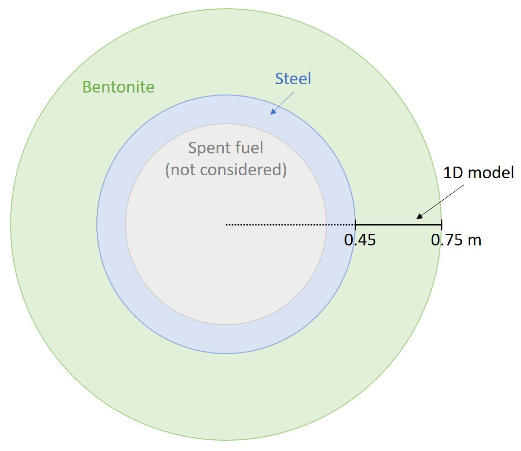
Figure 1.
Geometry and materials of the 1D radial model. The axisymmetric model only considers the canister-bentonite interface, at x = 0.45 m, and a thickness of 0.3 m of bentonite, from x = 0.45 to x = 0.75 m.
Figure 1.
Geometry and materials of the 1D radial model. The axisymmetric model only considers the canister-bentonite interface, at x = 0.45 m, and a thickness of 0.3 m of bentonite, from x = 0.45 to x = 0.75 m.
Figure 2.
Concentration of dissolved species in the porewater and of adsorbed species against distance for the reference model ( = 2 m ). The interface between steel and bentonite is at 0.45 m. Results after 5, 100, 1000 and 10,000 years of interaction are compared.
Figure 2.
Concentration of dissolved species in the porewater and of adsorbed species against distance for the reference model ( = 2 m ). The interface between steel and bentonite is at 0.45 m. Results after 5, 100, 1000 and 10,000 years of interaction are compared.
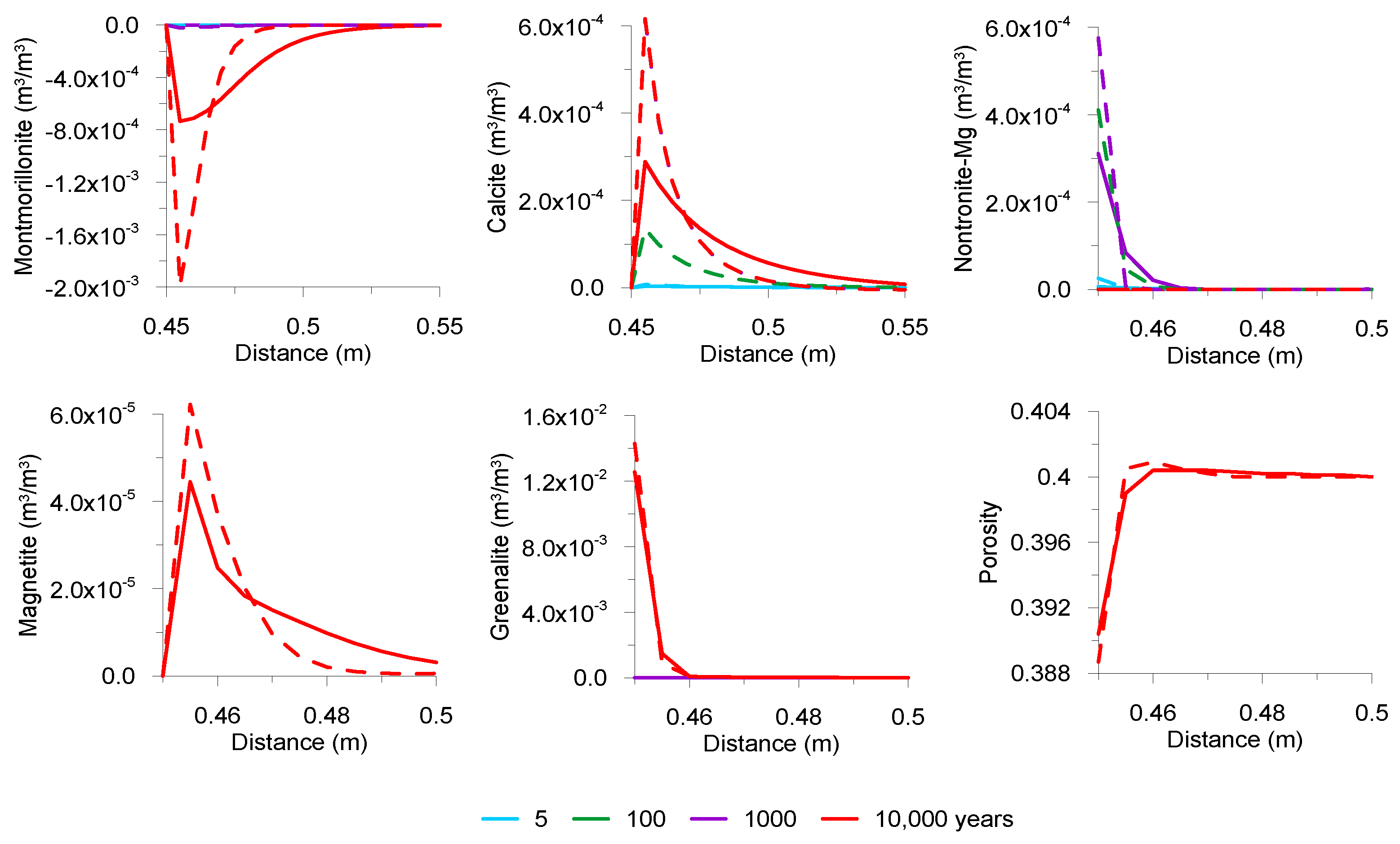
Figure 3.
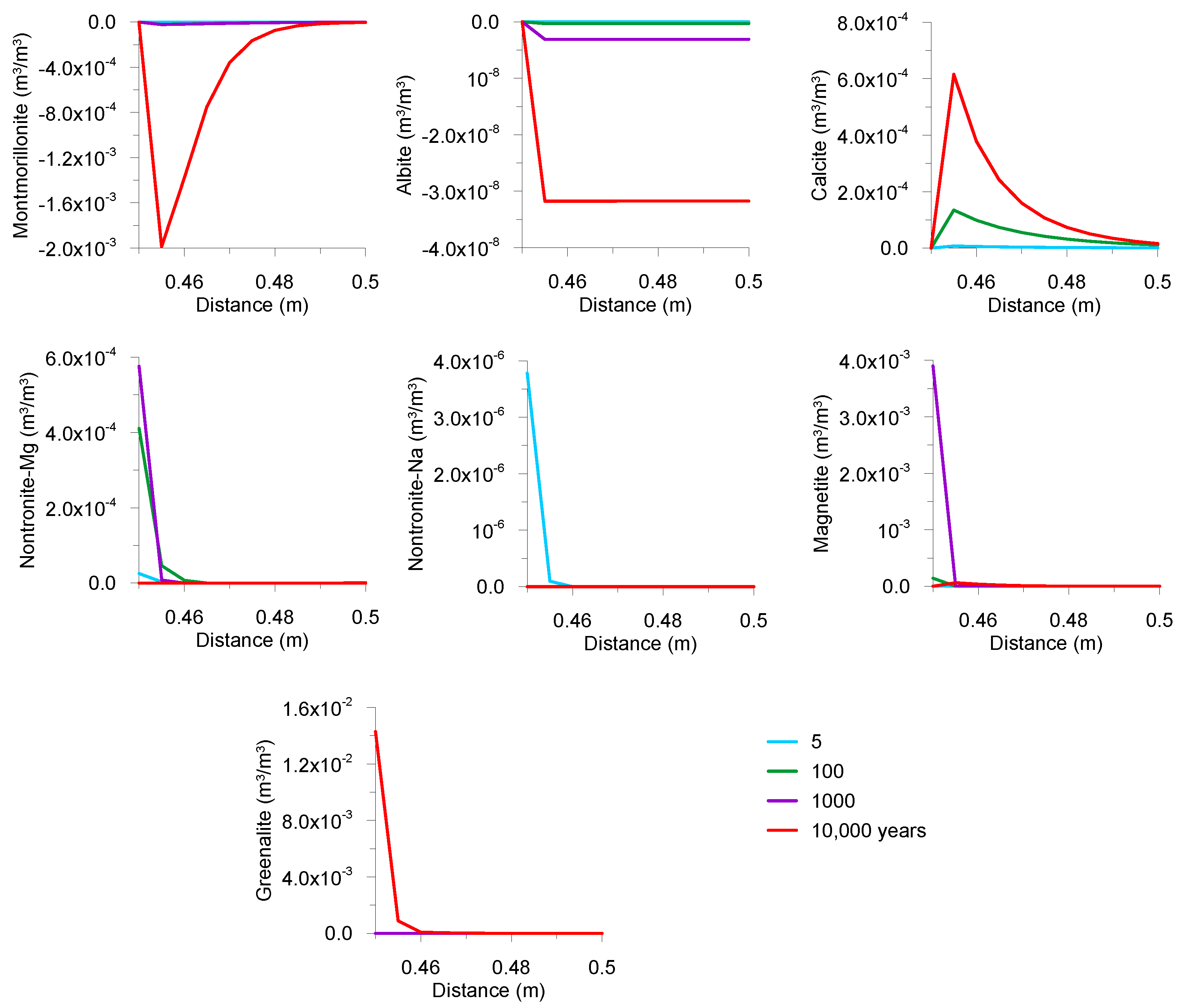
Volumetric fraction of minerals versus distance for the reference model ( = 2 m ). For the primary phases (montmorillonite, albite and calcite) the variation of the volumetric fraction is plotted. Positive values mean precipitation and negative values mean dissolution. The interface between steel and bentonite is at 0.45 m. Results at 5, 100, 1000 and 10,000 years of interaction are compared.
Figure 3.
Volumetric fraction of minerals versus distance for the reference model ( = 2 m ). For the primary phases (montmorillonite, albite and calcite) the variation of the volumetric fraction is plotted. Positive values mean precipitation and negative values mean dissolution. The interface between steel and bentonite is at 0.45 m. Results at 5, 100, 1000 and 10,000 years of interaction are compared.
Figure 4.
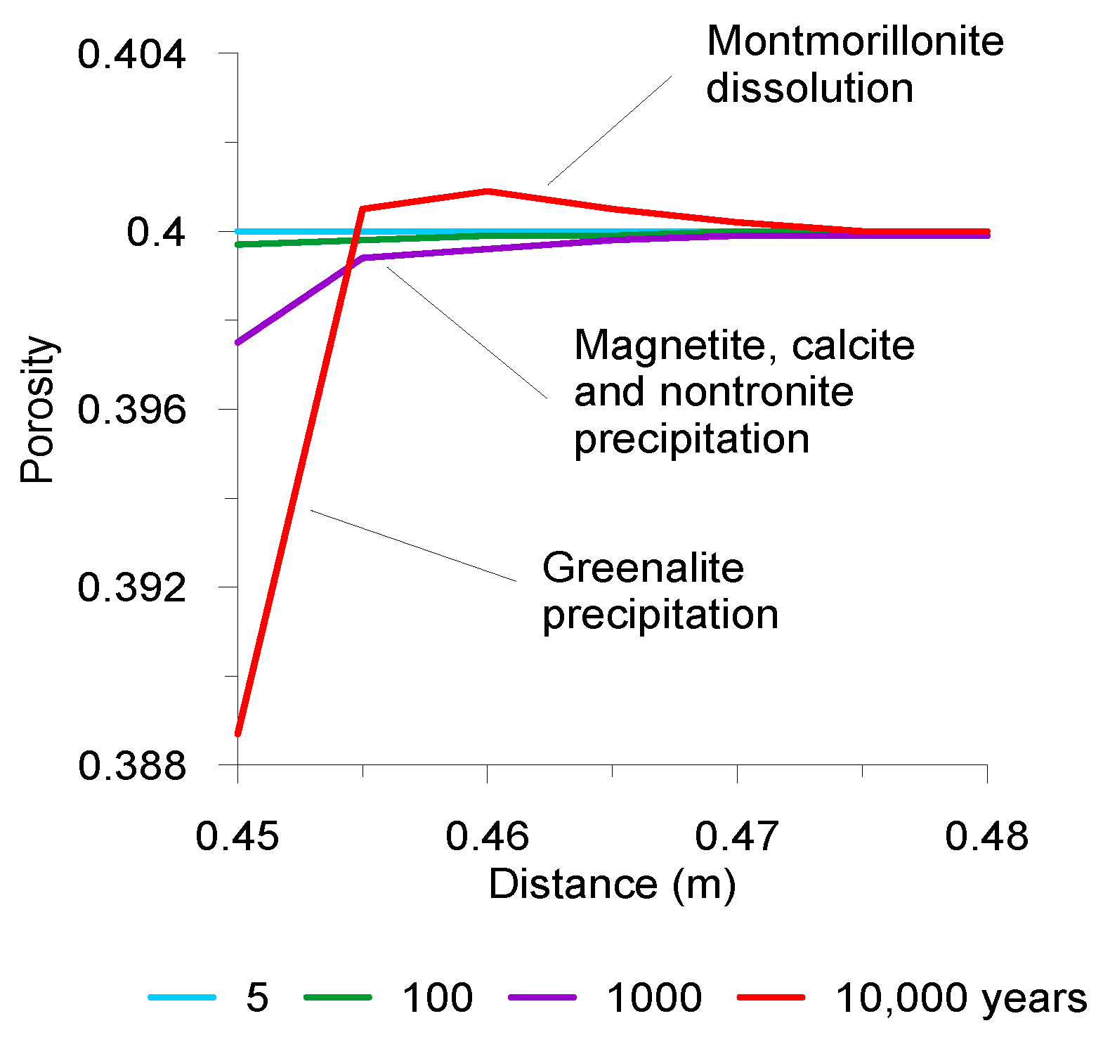
Porosity against length for the reference model ( = 2 m ). The interface between steel and bentonite is at 0.45 m. Results at 5, 100, 1000, and 10,000 years of interaction are compared.
Figure 4.
Porosity against length for the reference model ( = 2 m ). The interface between steel and bentonite is at 0.45 m. Results at 5, 100, 1000, and 10,000 years of interaction are compared.
Figure 5.
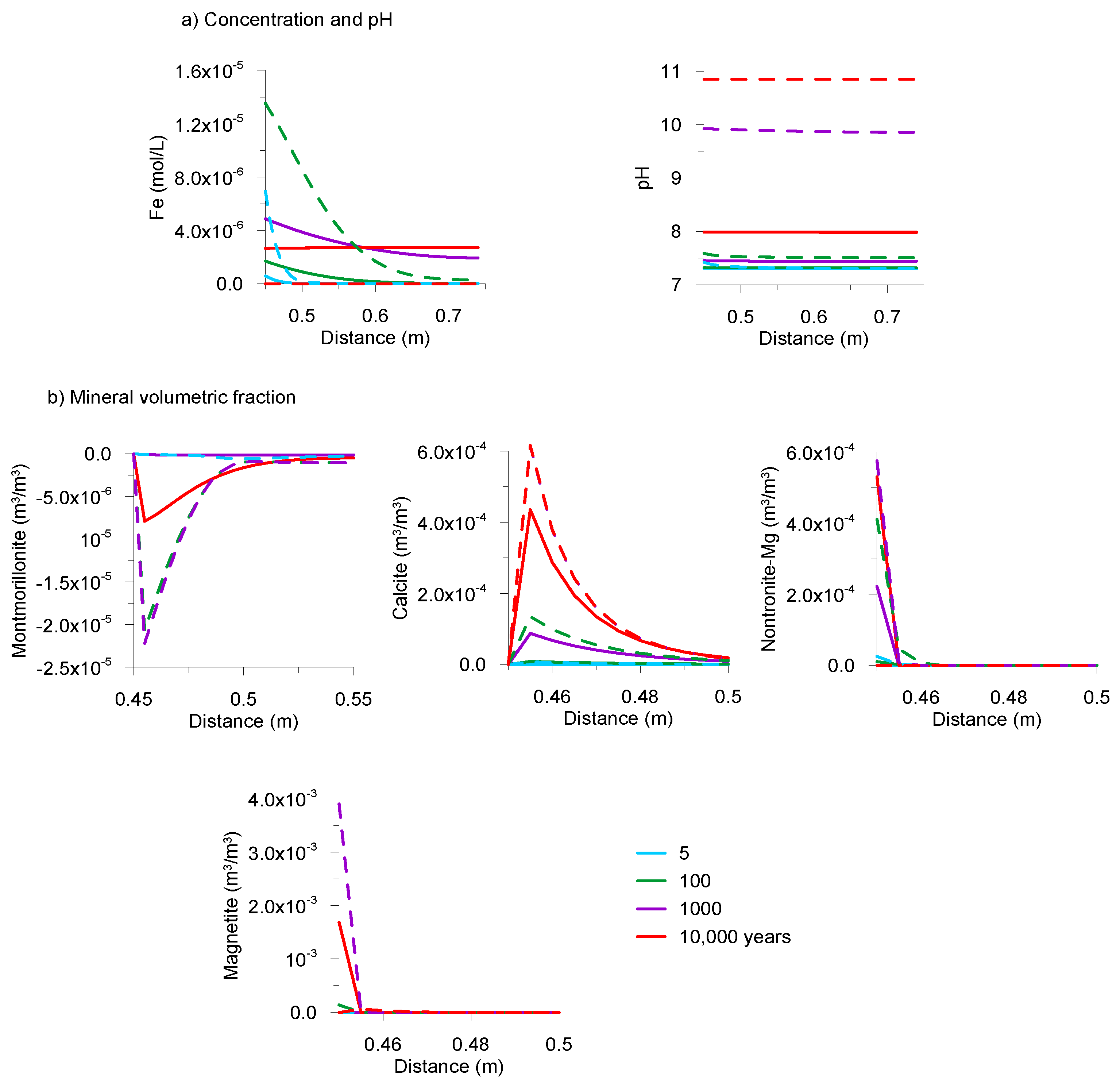
Results for the numerical model with a corrosion rate of 10 m (continuous lines) are compared with those from the reference model (r = 2 m , dashed lines). The interface between steel and bentonite is at 0.45 m. Results at 5, 100, 1000 and 10,000 years of interaction are given. (a) Fe concentration and pH against distance and (b) volumetric fraction of minerals versus distance. For the primary phases (montmorillonite and calcite) the variation of the volumetric fraction is plotted. Positive values mean precipitation and negative values mean dissolution.
Figure 5.
Results for the numerical model with a corrosion rate of 10 m (continuous lines) are compared with those from the reference model (r = 2 m , dashed lines). The interface between steel and bentonite is at 0.45 m. Results at 5, 100, 1000 and 10,000 years of interaction are given. (a) Fe concentration and pH against distance and (b) volumetric fraction of minerals versus distance. For the primary phases (montmorillonite and calcite) the variation of the volumetric fraction is plotted. Positive values mean precipitation and negative values mean dissolution.
Figure 6.
Results of the numerical model with a corrosion rate of 0.1
m
(continuous lines) are compared with those from the reference model (r = 2
m
, dashed lines). The interface between steel and bentonite is at 0.45 m. Results at 5, 100, 1000 and 10,000 years of interaction are compared. (
a) Fe concentration and pH against distance. (
b) Volumetric fraction of minerals versus distance. For the primary phases (montmorillonite and calcite) a variation of the volumetric fraction is plotted. Positive values mean precipitation and negative values mean dissolution. The reference model results for montmorillonite at 10,000 are not plotted (see
Figure 3 for that detail).
Figure 7.
Results of the numerical model with a diffusion coefficient of 6 ( = 2 m ) (continuous line) are compared with those from the reference model (dashed line). Volumetric fraction of minerals and porosity versus distance. For the primary phases (montmorillonite and calcite) the variation of the volumetric fraction is plotted. Positive values mean precipitation and negative values mean dissolution. The interface between steel and bentonite is at 0.45 m. Results at 5, 100, 1000 and 10,000 years of interaction are compared. For magnetite and porosity only results at 10,000 years are plotted.
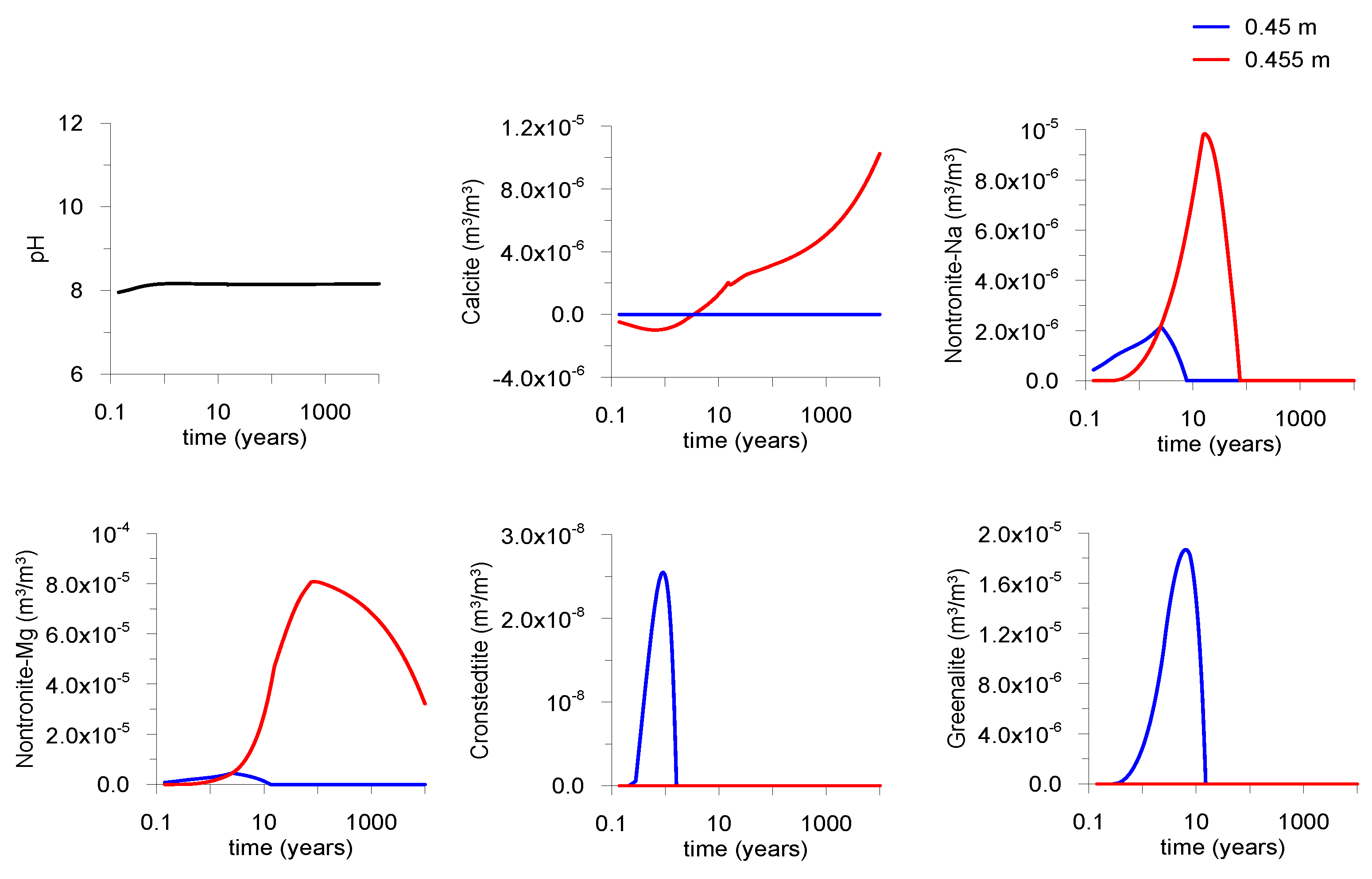
Figure 8.
Evolution of pH and volumetric fraction of secondary phases at two distances from the steel/bentonite interface considering a granitic porewater ( = 2 m ).
Figure 8.
Evolution of pH and volumetric fraction of secondary phases at two distances from the steel/bentonite interface considering a granitic porewater ( = 2 m ).
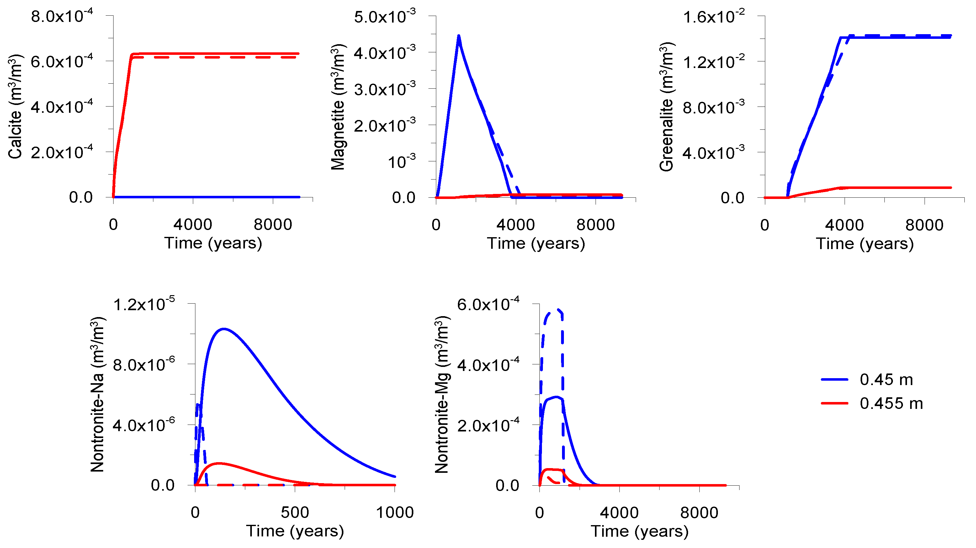
Figure 9.
Evolution of the volumetric fraction of the secondary phases of the model with a low reactive surface area ( = 0.1 /, continuous lines) compared with the reference model ( = 1000 /, dashed lines). Results of the node at the interface (0.45 m) and the node right after the interface (0.455 m) are plotted.
Figure 10.
Volumetric fraction of minerals of the model with 100,000 years interaction ( = 2 m ). For albite the variation of the volumetric fraction is plotted. Positive values mean precipitation and negative values mean dissolution. The interface between steel and bentonite is at 0.45 m. Results at 10,000 and 100,000 years of interaction are compared.
Table 1.
Comparison of the main differences in conceptual models between the present study and other reported models in the literature.
Table 1.
Comparison of the main differences in conceptual models between the present study and other reported models in the literature.
| | Present Study | Bildstein et al. [13] | Wilson et al. [18] | Samper et al. [19] |
|---|
| Geometry | Canister as boundary | Porous canister | Canister as boundary and porous canister | Porous canister |
| Temperature | 25 | 50 | 70 | 25 |
| Bentonite | MX-80 | MX-80 | MX-80 | FEBEX |
| Secondaryphases | Magnetite, nontronite greenalite, siderite cronstedtite | Magnetite, siderite, chamosite, saponite cronstedtite | Magnetite, siderite amesite, berthierine chlorite, greenalite, lizardite, analcime, cronstedtite, saponite | Magnetite, siderite analcime, cronstedtite |
| Corrosion rate | 2 m | 4.3 m | 1 m | 2 m |
| Interaction time | 10,000 y | 16,250 y | 10,000 y | 1 y |
Table 2.
Bentonite mineralogical composition considered in the numerical model. The volumetric fractions are also listed for each phase.
Table 2.
Bentonite mineralogical composition considered in the numerical model. The volumetric fractions are also listed for each phase.
| Mineral | Volumetric Fraction () |
|---|
| Montmorillonite | 5.01 |
| Quartz | 4.70 |
| Albite | 2.10 |
| Muscovite | 2.10 |
| Illite | 5.00 |
| Pyrite | 4.00 |
| Calcite | 1.00 |
Table 3.
MX-80 bentonite initial porewater composition used in the numerical model. Imposed constraints to calculate some of these values (equilibrium with solids and charge balance) are also indicated.
Table 3.
MX-80 bentonite initial porewater composition used in the numerical model. Imposed constraints to calculate some of these values (equilibrium with solids and charge balance) are also indicated.
| Component | Water Composition (mol ) |
|---|
| 2.00 |
| 8.60 |
| 3.54 charge balance |
| 7.19 |
| 1.31 calcite |
| 2.50 |
| 6.50 |
| 7.30 |
| (aq) | 1.00 |
| 1.70 |
| (aq) | 1.00 |
| pH | 7.30 |
Table 4.
Equilibrium constants (log at 25) of the minerals taken into account in the numerical model. Reactions are written as the dissolution of 1 mol of mineral in terms of the primary species , , (aq), , , , , , , , and (aq).
Table 4.
Equilibrium constants (log at 25) of the minerals taken into account in the numerical model. Reactions are written as the dissolution of 1 mol of mineral in terms of the primary species , , (aq), , , , , , , , and (aq).
| Mineral | Formula/Reaction | log |
|---|
| Iron | Fe(s) + 2 + 0.5(aq) = + O | 59.01 |
| Montmorillonite | | −18.02 |
| Quartz | | −4.00 |
| Albite | | −19.39 |
| Muscovite | | −52.86 |
| Illite | | −41.92 |
| Pyrite | | 217.34 |
| Calcite | | 1.85 |
| Magnetite | | −6.51 |
| Greenalite | | 22.65 |
| Cronstedtite | | −0.73 |
| Nontronite-Na | | −35.82 |
| Nontronite-Mg | | −35.92 |
| Siderite | | −0.19 |
Table 5.
Secondary species with their equilibrium constants (log at 25) taken into account in the numerical model. Reactions are written as the dissolution of 1 mol of mineral in terms of the primary species , , (aq), Al, , , , , , , and (aq).
Table 5.
Secondary species with their equilibrium constants (log at 25) taken into account in the numerical model. Reactions are written as the dissolution of 1 mol of mineral in terms of the primary species , , (aq), Al, , , , , , , and (aq).
| Formula | log | Formula | log |
|---|
| Al(aq) | −5.99 | Fe | 13.12 |
| Al | −11.55 | Fe | −2.59 |
| Al | −17.18 | Fe( | −11.73 |
| −22.14 | (aq) | −2.19 |
| (aq) | 7.01 | | −14.02 |
| (aq) | −2.10 | | −1.98 |
| 12.85 | | 138.27 |
| 0.70 | | 13.99 |
| −1.04 | (aq) | 7.35 |
| (aq) | 0.65 | | −1.03 |
| 8.79 | (aq) | −2.38 |
| 10.32 | | 11.78 |
| (aq) | −6.34 | | 0.14 |
| −8.48 | | 8.54 |
| −2.04 | NaOH(aq) | 14.79 |
| (aq) | 5.53 | | 9.82 |
| −0.16 | (aq) | −0.15 |
| −7.67 | NaCl(aq) | 0.78 |
| (aq) | 2.46 | | −0.81 |
| 9.63 | KCl(aq) | 1.50 |
| −6.29 | KOH(aq) | 14.46 |
| Fe(aq) | 20.59 | | −0.87 |
| Fe(aq) | 3.64 | | |
Table 6.
MX-80 bentonite cation exchange reactions and log K at 25
[
38].
Table 6.
MX-80 bentonite cation exchange reactions and log K at 25
[
38].
| Exchange Reaction | log K |
|---|
| 2NaX + = 2 + | 0.80 |
| 2NaX + = 2 + | 0.50 |
| 2NaX + = 2 + | 0.60 |
| NaX + = + KX | 0.70 |
Table 7.
Reactive surface areas and kinetic constants (at 25
) of the primary minerals considered in the bentonite and the possible corrosion products. (a) Cama et al. [
40] (b) Bildstein et al. [
13] (c) Dove [
41] (d) Knauss and Wolery [
42] (e) Kamei and Ohmoto [
43] (f) Plummer et al. [
44] (g) Wilson et al. [
18].
| Mineral | (/) | (mol/s) | References () |
|---|
| Montmorillonite | 1 | 1.58 | (a,b) |
| Quartz | 0.01 | 1.00 | (c,b) |
| Albite | 0.01 | 1.00 | (d,b) |
| Muscovite | 0.01 | 1.58 | Montmorillonite analogue |
| Illite | 0.01 | 1.58 | Montmorillonite analogue |
| Pyrite | 0.01 | 5.01 | (e,b) |
| Calcite | 0.01 | 6.31 | (f,b) |
| Magnetite | 1 | 4.47 | (g) |
| Greenalite | 1 | 4.90 | (g) |
| Cronstedtite | 1 | 1.58 | (b) |
| Nontronite-Na | 1 | 1.58 | Montmorillonite analogue |
| Nontronite-Mg | 1 | 1.58 | Montmorillonite analogue |
| Siderite | 1 | 1.00 | (b) |
Table 8.
Initial porewater composition used in the sensitivity analysis.
Table 8.
Initial porewater composition used in the sensitivity analysis.
| Component | Water Composition (mol ) |
|---|
| Al | 1.00 |
| 1.52 |
| 3.95 |
| 1.79 |
| 5.05 |
| 5.37 |
| 1.60 |
| 4.35 |
| (aq) | 3.76 |
| 1.56 |
| (aq) | 1.00 |
| pH | 7.83 |


