Concealed-Fault Detection in Low-Amplitude Tectonic Area—An Example of Tight Sandstone Reservoirs

Abstract

Fault detection is important to seismic interpretation, especially for tight oil and gas reservoirs. Generally speaking, large-scale faults can be accurately imaged and are easy to detect by conventional methods, but the concealed ones in low-amplitude structural regions are difficult to find. In these areas, the scale and displacement of concealed faults are usually very small. Due to the good uniform and weak amplitude disturbances in the seismic events, the traditional discontinuity attributes extracted from seismic data are always not effective. This is because the discontinuous features of large faults are very significant, and the weak anomalies caused by hidden faults are very close to the continuous background. This paper takes a tight sandstone reservoir in the Ordos Basin of China as an example to explore the detection method of subtle faults in low-amplitude structural areas. With the phase congruency analysis method, we extract edge features from the post-stack coherence attributes to identify hidden faults. Practice shows that this idea has outstanding performance in mining hidden fracture features and improving the accuracy of fracture recognition. The results successfully predict a shear fault zone in the northeast of the work area, find a new fracture zone in the center of the survey and a series of hidden faults in non-target strata. It would be beneficial to extend the strata and area of oil and gas reservoirs.

1. Introduction

Fault detection helps us to understand basic factors of oil and gas accumulation such as reservoir formation, migration and preservation. It is becoming more and more challenging as the requirements for exploration accuracy increase. Conventional post-stack discontinuity extractions are the main technologies of fault detection, such as eigenvalue-based coherence [1,2,3] and curvature [4,5,6]. These methods could indicate dislocation, shape change, bifurcation, merging, and distortion of the seismic event caused by faults and, therefore, are widely used. The data basis of these methods is the contrast of amplitude between adjacent seismic traces. The amplitude at the faults depends on the scale, the degree of fragmentation of surrounding rock, the fold number in the field, the illumination angle, the choice of imaging method, and the size of the migration aperture. Generally, large-scale faults can be accurately imaged and are easy to detect, but the concealed ones in low-amplitude structural regions are difficult to find. The opposite is that the negative features such as small fault distance and weak contrast between adjacent traces lead to low accuracy or even the total failure of conventional technologies. Identifying those fuzzy and weak fault features accurately and completely has become a difficulty that researchers must confront.

Without additional seismic imaging work, previous researchers attempted to overcome the above-mentioned problems and achieved significant progress in five aspects. Firstly, optimizing geological structures to improve fault resolution, such as structure-oriented filtering technologies [7,8,9,10,11]. Secondly, extracting the fault characteristics of the dominant frequency band through frequency division such as frequency division coherence [12,13] and frequency division curvature [14]. Thirdly, obtaining more distinguished fault characteristics by direction and scale enhancement [15]. Fourthly, discontinuity optimization, such as ant tracking [16,17], maximum likelihood attribute [18,19] and histogram enhancement [20,21]. Fifth, deep learning methods based on the seismic waveform and neural networks [22,23,24]. These methods may be the most promising technologies in recent years. They can detect faults based on pre-set seismic data label features (such labels can be manually selected or set through forward simulation). Someday in the future, these methods even can find every fault that has ever appeared in the minds of geologists. However, the current deep learning technologies are still not smart enough and cannot recognize the fault patterns until we “teach it”. In the real underearth, the possible shapes, scales, and distribution characteristics of faults must be far beyond our minds. These methods will likely miss some faults, even if they are important.

In summary, the above-mentioned ideas and techniques have largely made up for the shortcomings of conventional post-stack attribute technologies and greatly improved the accuracy of fault identification. However, in general, these works are carried out around the “amplitude” of seismic waves. Therefore, the identification accuracy is still severely constrained by the amplitude contrast between the adjacent traces.

To obtain better effects on existing data, we may consider avoiding dependence on the amplitude variations of adjacent seismic traces. In image processing, the phase retained the edges and the overall structures, which are the most essential characteristics of images other than the amplitude, and this has attracted much attention [25]. The edges and corners obtained from the image phase are far more reliable than the ones calculated from intensity alone. In this paper, the concept of phase congruency (PC) in image processing was introduced to enhance the discontinuities of concealed faults. The PC extracted from eigenvalue-based coherence attributes could change the relatively weak discontinuities to stronger states.

2. Methods and Tests

2.1. Method

In image cognition, the edges and corners are the key features of the image. Early feature extractions were mainly based on image intensity gradients, such as the Sobel operator [26,27], the Marr operator [28], and the Canny operator [29]. These methods were very sensitive to image brightness and contrast and useful in fault detection of seismic exploration [30,31]. However, any gradient-based edge detection process will need to use a threshold that is modified appropriately. However, the prior knowledge of overall brightness is generally unknown. The more complex the image structures, the more difficult the threshold adjustments that are required, and thus, the worse the edge detection that will be obtained.

In 1986, the local energy model proposed by Morrone and Owens broke the limitation of the above methods, postulating that the image edges and corners correspond to the maximum PC of the pixels [32]. The approach of calculating maximum PC by searching for peaks in the local energy function proposed by Venkatesh and Owens [33] has been widely adopted. Then, Kovesi used a 2-D Log-Gabor filter with multi-scale, multi-azimuth, and zero direct-current (DC) component characteristics to successfully implement the PC analysis of the 2-D image. The edges and corners obtained from the above method remained relatively stable with the invariance of brightness and contrast, thus greatly expanding the development and application of the theory [34,35,36,37]. The core theoretical formula of two-dimensional PC proposed by Kovesi (2003) can be written as

$$PC(x_1,x_2)=\frac{{\displaystyle {\sum }_s{\displaystyle {\sum }_{o}W(x_1,x_2)\lfloor A_{so}(x_1,x_2)\Delta {\Phi }_{so}(x_1,x_2)-T\rfloor }}}{{\displaystyle {\sum }_s{\displaystyle {\sum }_o{A}_{so}(x_1,x_2)}+\epsilon }}$$

(1)

$$\Delta {\Phi }_{so}(x_1,x_2)=\cos ({\varphi }_{so}(x_1,x_2)-\overline{\varphi }(x_1,x_2))-\left|\sin ({\varphi }_{so}(x_1,x_2)-\overline{\varphi }(x_1,x_2))\right|$$

(2)

where PC(x₁, x₂) denotes the PC value located in (x₁, x₂), and is a dimensionless quantity varying from 0 to 1, which means that the image has no feature to a significant feature; W(x₁, x₂) is the weight function for frequency spread, which may vary with frequency. A_so(x₁, x₂) the amplitude at scale s and orientation o; ${\varphi }_{so}(x_1,x_2)$ is the phase angle; $\overline{\varphi }(x_1,x_2)$ is the weighted mean phase angle; T is noise threshold; ε is a small constant avoiding division by zero; “$\lfloor \rfloor$“ denote that the enclosed quantity is equal to itself when its value is positive, and is zero otherwise.

The most important steps to calculate PC are the following:

(1)

Calculate the multi-scale and multi-orientation log-Gabor filter bank in the frequency domain;

(2)

Calculate the Fourier transform of the coherence slice;

(3)

Convolve the results in step (2) with all multi-scale and multi-orientation filters, and calculate the Inverse Fourier transform;

(4)

Extract the total energy by summing the scale-dependent absolute amplitude obtained in step (3) in each orientation. Researchers can obtain the denominator in formula (1) in this step;

(5)

Follow step (3) to calculate the energies of even and odd versions, obtain their square root of amplitude, and count the weighted mean phase angles;

(6)

Compute the sigmoidal weighting function for each orientation;

(7)

Calculate numerator in formula (1);

(8)

Compute the PC for each orientation;

(9)

Extract some characteristics from the PC such as the feature phase and the maximum moment.

A more detailed description can be found in Kovesi’s paper [35,37].

The phase congruency analysis has the characteristics of contrast invariance and does not rely on local changes in illumination. Therefore, it has an excellent performance in image feature extraction. This method is widely used in visual analysis [38], image fusion [39], image reconstruction [40], image quality evaluation [41], image registration [42] and other non-image processing fields; for example, seismic interpretation in oil and gas exploration. Russell et al. applied the PC algorithm to detect karst collapse and fractures in carbonate [43]. Kovesi et al. extended PC to a 3D algorithm for velocity anomalies and the detection of hidden fault edges in seismic data [44]. Shafiq et al. highlighted the use of a salt dome with the PC method [45]. Taking inspiration from PC, Karbalaali et al. used a shearlet transform to identify channel edges [46]. These cases presented the great potentiality of PC in directly extracting some large-scale discontinuities from the original seismic amplitude.

However, directly extracting discontinuities from seismic amplitude is not an ultimate strategy for fault detection. Some tiny changes in seismic amplitude and original attributes such as coherence are difficult to attract the attention of engineers. The micro-faults and fractures in low-amplitude tectonic areas are a source of endless annoyance for engineers. This problem is really common in many tight sandstone reservoirs in West China. In fact, the ant tracking and likelihood attribute methods have already reminded us that optimizing distribution or re-extracting edges from conventional attributes can achieve better results. In next section, the authors conducted experiments using model data. We tried to extract the PC attribute from artificial coherence images and also hoped that this test could demonstrate the capabilities of the PC method in concealed fault detection.

2.2. Tests

It is well known that the PC algorithm is suitable for edge detection of ordinary images. Next, the potentiality of PC for fault detection from seismic attributes will be discussed in detail. Figure 1 shows two examples of model data. Given a coherence slice of grid size 100 × 100 and the background value of 1, it can be assumed that the stratum was flat enough, and the seismic events extended horizontally with no jitter, dislocation, or deflection. Two orthogonal faults f₁ and f₂ were designed in this model and tested in two ways. In the first experiment (as shown in Figure 1a), the coherence value on f₁ changed from 1 to 0.9 with a linear step of 0.001. This was a very small change rate to the background value. The coherence values on f₂ stayed at 0.999 before x₁ = 30, which means the differences caused by the fault were weak and stable. On the other part (x₁∈[31, 100]) of f₂, coherence changed from 0.999 to 0.929 by the step of 0.001, which means the faults edges became slowly sharpened. In the second experiment, fault f₂ remained the same, and fault f₁ was changed with a random value from 0.99 to 1.0, as shown in Figure 1c. The continuity of f₁ was severely destroyed.

Figure 1b,d show us the phase congruencies of Figure 1a,c respectively. The comparison shows that this method has the following characteristics. Firstly, stable and continuous changes in coherence value, even if the contrast is very small (the gradient is one thousandth in this test), could be precisely identified as faults by phase congruency, such as fault f₁ and f₂ shown in Figure 1a,b. Secondly, rapid and irregular changes of coherence values may lead to inconspicuous fault characteristics, but could still be located accurately and clearly by their PC, such as fault f₁ shown in Figure 1c,d. Thirdly, the result obtained near the intersection of the faults may be unsatisfactory, as shown in Figure 1d. The reason is unknown. Thus, more attention should be paid to the areas where the faults are staggered. On the whole, the PC is very sensitive to discontinuous features such as weak misalignment of seismic events caused by concealed faults and can be used effectively to improve the recognition accuracy.

In seismic interpretation, the spatially discontinuous boundaries of the seismic attribute are usually suspected as faults. Therefore, the above tests show the suitability of the phase congruency for extracting fault boundaries. In addition, this method is sensitive to both the boundaries and the noise. However, this article is aimed at the detection of small faults in low-amplitude structural areas close to the horizontally layered uniformity. Such areas generally have very high imaging quality and low noise levels, so that this disadvantage can be ignored.

3. Application

3.1. Background

The research area is located in the northern section of the Ordos Basin, China. To its west is the western edge of the thrust belt of the basin. Its structural shelf diagram is shown in Figure 2. The study area (marked with the red frame) is mainly located outside the thrust belt, without any deep and large faults developed. According to previous research, the faults developed in the target stratum belong to the regional low-order faults, mainly dominated by the overthrust nappe controlled by the main curtain of the Yanshan Movement. They are formed under the combined effects of strike-slip stress and paramount fault traction. Their typical features are small fault distance, short extension and small scale. The lower-order faults were later transformed by the Himalayan movement after the formation. However, the nature of the faults has remained unchanged, and the seismic reflection event axis rarely exhibits features such as structural reversal. The faults are still dominated by reverse faults formed by the main curtain of the Yanshan period. In addition, the study area suffers from less uplift and denudation of strata, and the influence of later tectonic movement on lower-order faults is limited. It could be seen that since the formation, these low-level sequence faults have been in a relatively static state for an extended period of geological history. This is very positive to reservoirs.

Figure 3 is target horizon map of the study area shown in the red frame in Figure 2. It is the zoomed-in version. It can be seen that the target layer is higher in the west and lower in the east. The structural range presents a distinct band distribution from southwest to northeast. From north to south, the structural stress gradually weakened, the structural amplitude gradually decreased, and the horizon extended approximately horizontally. The terrain in the middle and northeast of the study area is flat, and the horizontal continuity and amplitude congruency of the seismic event are the best, as shown in Figure 4.

The white area represents the young graben system around basin margins, and dark gray represents the deformation belts around the Ordos basin. 1—fault; 2—normal fault; 3—thrust fault; 4—strike-slip fault; 5—fold; 6—river; 7—city; 8—basin boundary; 9—tectonic unit boundary; 10—study area.

3.2. Problem

In the study area, there are three typical wells, namely w1, w2, and w3. Their locations are shown in Figure 3. Figure 5 shows their statistics of the fractures in the target zone. They are sorted according to the number of cracks, in the order of w2 > w3 > w1. In addition, the fractures in Wells w2 and w3 are all high-angle fractures, while well w1 mainly exhibits high-angle fractures, supplemented by medium-angle fractures and a small number of low-angle fractures. Based on this, geologists judged that the above three wells are all located in the fracture zone.

The coherence attributes of the target horizon (see Figure 6a) show us two apparent groups of low-order fault zones in this area. They are divided by red dotted lines. Zone Ⓐ is a tensile fault zone that almost runs northwest–southeast, and is stretched to the south and north. Zone Ⓑ is a mass of obvious zoning tensile faults composed of sets of echelon fractures close to the EW and NWW to SE directions. This point can be clearly seen from the local coherence in the blue frame labelled with the number “1”. The development of the above sectional faults is consistent with the geological understanding and the well fractures. In addition, according to the existing geological knowledge, there should be a fault belt in the upper right corner of this stratum. It was sheared due to fault zone Ⓑ and we named it zone Ⓒ. The fractures in the well w3 confirm the potential rationality of this inference (shown in Figure 5). However, the coherences in zone Ⓒ are so fuzzy that they fail to give sufficient evidence to support the above inference. Typically, the area in blue frame named with number “2” in Figure 6a could hardly give us any valuable information.

From the analysis of amplitude and coherence profile, the authors believe that the failure of fault prediction was caused by the superposition of two factors. Firstly, the target stratum is located in the low-order fault development zone of the Ordos Basin, and its overall structural amplitude is already very gentle. Secondly, well w3 is located in the relatively “low” structural area of the target stratum, which further reduces the horizon gradient. Under the double superimposition, the seismic event continuities in zone Ⓒ, where well w3 is located, were found to be very good. The seismic amplitude disturbances caused by the concealed faults were judged to be too weak to be helpful for fault identification via coherences. Mining of the weak discontinuous features of hidden faults and improving the recognition rate is a key issue for interpreters.

3.3. Result

To solve the above problems, the author extracted the PC as discontinuities from the coherence to detect the concealed faults, and the results are presented in Figure 6b. Comparing Figure 6a,b, interpreters could gain five clear understandings. Firstly, the features of the main faults remained basically the same before and after reinforcement, and were consistent with the laws of geology. This highlights the reliability of phase congruency. Secondly, the discontinuities enhanced by the PC show higher resolution than the coherent attribute. Thirdly, the PC connected broken related discontinuities into local integral faults and effectively expanded their trend in space. These observations provided some new knowledge on the fault ranges in zone Ⓐ and Ⓑ. Fourthly, faults located in the upper right corner that were sheared as a result of those in zone Ⓑ were perfectly distinguished. The main fault zone spread from northeast to southwest, and was associated with some secondary faults in the north–south direction. Therefore, zone Ⓒ can be regarded as another fault development area. This reasonably explains why the fractures developed in well w3. Based on this new and reliable evidence, geologists finally demonstrated the existence of a shear strike-slip fault zone with a small displacement in the northern part of the survey. In addition, this point may expand the area of potential high-quality tight sandstone reservoirs to the north and the east. Finally, the results also show that there was a fault zone named Ⓓ in the center of the area, slightly to the south. Obviously, this was the stress relief area of the three fault zones. Therefore, the fault scale was smaller and more complex.

For further confirmation of the authenticity of the fault features, the amplitude profile and discontinuities of an arbitrary line (the red line shown in Figure 6) were extracted. Then, the discontinuities were displayed over the amplitude via the adjustment of the transparency. There were five typical areas for comparison, section ①, section ②, section ③, section ④, and section ⑤, which were limited to the blue boxes, as shown in Figure 7. Among them, section ① and section ② were located near the target stratum. Section ① passed through the area in blue frame, labelled with the number “1”, in fault zone Ⓑ. The main faults were so sharp that the misalignments that occurred in the events were sufficiently clear before and after enhancement due to large fault distances. The fault features in the slice (Figure 6b) were consistent with the ones in the profile (Figure 7b). In this situation, the faults could be considered real. Section ② passed through the area in the blue frame, labelled with the number “2”, in fault zone C. There were some slight deflections in the events here. The coherence slices shown in Figure 6a and profile in Figure 7a had almost no clear response to faults. In contrast, the fault features were clearly identifiable in the PC results for the slice and the profile, as shown in Figure 6b and Figure 7b.

Section ① and section ② were near the target stratum, and section ③ to ⑤ were near the X-stratum.

Similar situations existed in other strata. Discontinuities of concealed faults in section ③, section ④, and section ⑤ yielded the following comparisons. Overall, they were all flexural faults with slight deformations in their events, especially the patterns in section ⑤. These event variations were too slight to be detected by coherence, as shown in Figure 7a. However, the PC attributes effectively enhanced the discontinuity magnitude and still precisely identified the concealed faults.

4. Conclusions

In this paper, the phase congruency method was introduced to enhance the fault features presented by coherence. The experiments conducted using model data and filed data in the low-amplitude structure area proved that this method is an effective tool for detecting concealed faults. The following insights were obtained:

(1)

The phase congruency method focuses more on the “location” of faults rather than the discontinuity values. For this reason, this method is equally sensitive to effective information and noise and should be combined with geological structures to eliminate unnecessary disturbances.

(2)

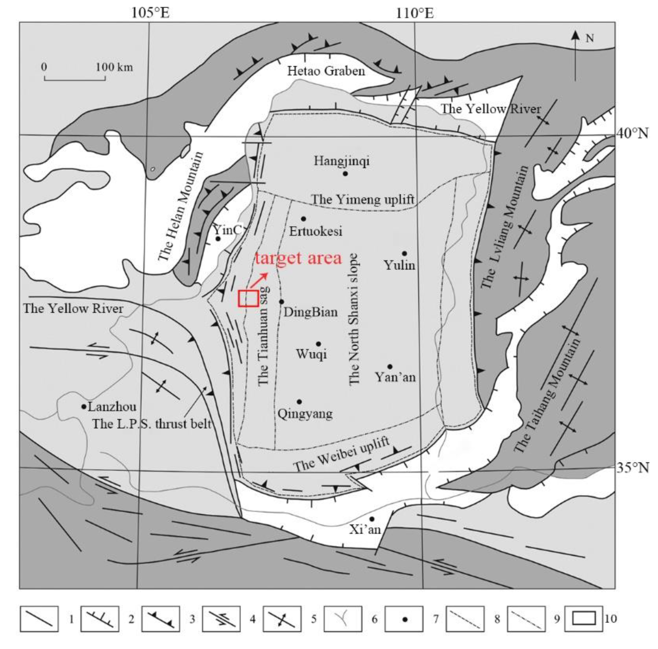
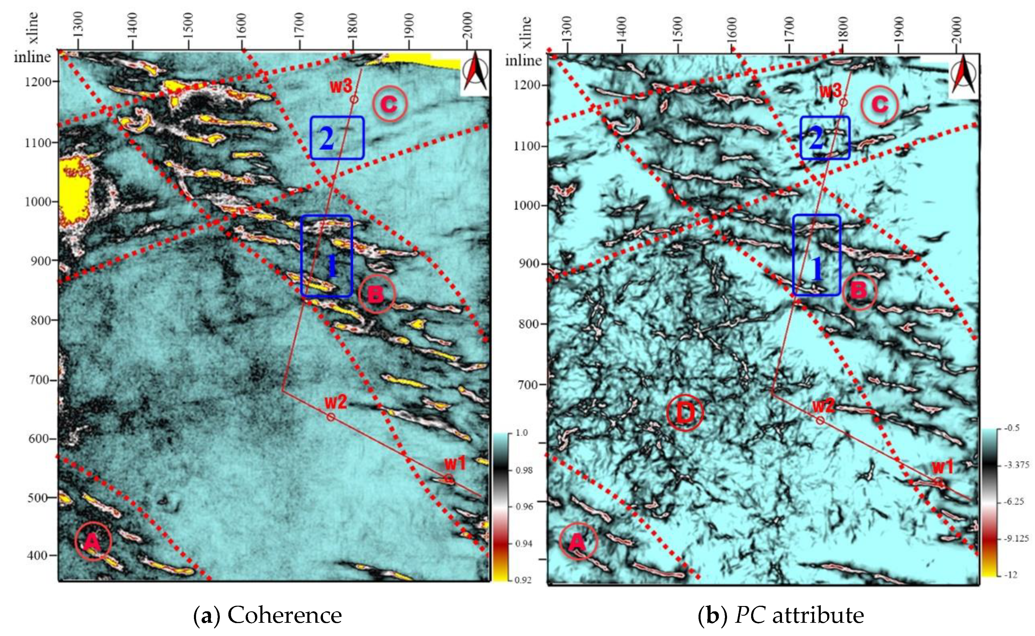
The study area mentioned in this paper is located in the low-amplitude structural area of the Ordos Basin in China, formed from the Late Jurassic to the end of the Early Cretaceous period and earlier than the main accumulation period of Mesozoic oil reservoirs. Hidden faults with small fault distances and small spatial extensions are difficult to detect with conventional methods. Using the phase congruency analysis method, we first helped geologists to demonstrate the existence of a shear fault zone in the northeast of the work area. This has a positive significance in terms of expanding the area of high-quality reservoirs to the north and east. Second, a new and vast fracture zone in the center of the survey, slightly to the south, was found. It is the stress relief area of different fault zones and likely has more crossed-fracture networks. This is a positive development in terms of providing the necessary oil or gas channels in tight sandstone reservoirs. Thirdly, a series of hidden faults in other strata were newly discovered. Some of these faults influence the bottom water, causing water to flow out during the process of testing for oil, which decreases the recovery rate; some faults form effective channels, improve the overall permeability of the reservoir, and contribute to accumulation. This research is of great significance for understanding the law of oil and gas migration and avoiding the risk of leakage caused by fracturing.

References

1. Gersztenkorn, A.; Marfurt, K.J. Eigenstructure-based coherence computations as an aid to 3-D structural and stratigraphic mapping. Geophysics 1999, 64, 1468–1479. [Google Scholar] [CrossRef]
2. Marfurt, K.J.; Sudhaker, V.; Gersztenkorn, A.; Crawford, K.D.; Nissen, S.E. Coherency calculations in the presence of structural dip. Geophysics 1999, 64, 104–111. [Google Scholar] [CrossRef]
3. Cohen, I.; Coifman, R.R. Local discontinuity measures for 3-D seismic data. Geophysics 2002, 67, 1933–1945. [Google Scholar] [CrossRef]
4. Roberts, A. Curvature attributes and their application to 3D interpreted horizons. First Break 2001, 19, 85–100. [Google Scholar] [CrossRef]
5. Al-Dossary, S.; Marfurt, K.J. 3D volumetric multispectral estimates of reflector curvature and rotation. Geophysics 2006, 71, P41–P51. [Google Scholar] [CrossRef]
6. Hakami, A.M.; Marfurt, K.J.; Al-Dossary, S. Curvature attribute and seismic interpretation: Case study from Fort Worth Basin, Texas, USA. In SEG Technical Program Expanded Abstracts 2004; Society of Exploration Geophysicists: Tulsa, OK, USA, 2004; pp. 544–547. [Google Scholar] [CrossRef]
7. Weickert, J.; Scharr, H. A Scheme for Coherence-Enhancing Diffusion Filtering with Optimized Rotation Invariance. J. Visual Commun. Image Represent. 2002, 13, 103–118. [Google Scholar] [CrossRef] [Green Version]
8. Fehmers, G.C.; Höcker, C.F.W. Fast structural interpretation with structure-oriented filtering. Geophysics 2003, 68, 1286–1293. [Google Scholar] [CrossRef]
9. Hale, D. Structure-oriented smoothing and semblance. In CWP Report 635; Center for Wave Phenomena, Colorado School of Mines: Golden, CO, USA, 2009; pp. 261–270. [Google Scholar]
10. Hale, D. Structure-oriented bilateral filtering of seismic images. In SEG Technical Program Expanded Abstracts 2011; Society of Exploration Geophysicists: Tulsa, OK, USA, 2011; pp. 3596–3600. [Google Scholar] [CrossRef]
11. Wang, J.; Chen, Y.; Xu, D.; Qiao, Y. Structure-oriented edge-preserving smoothing based on accurate estimation of orientation and edges. Appl. Geophys. 2009, 6, 367–376. [Google Scholar] [CrossRef]
12. Partyka, G.; Gridley, J.; Lopez, J. Interpretational applications of spectral decomposition in reservoir characterization. Lead. Edge 1999, 18, 353–360. [Google Scholar] [CrossRef] [Green Version]
13. Wang, X.W.; Yang, K.Q.; Zhou, L.H.; Wang, J.; Liu, H.; Li, Y.M. Methods of Calculating Coherence Cube on the Basis of Wavelet Transform. Chin. J. Geophys. 2002, 45, 847–852. [Google Scholar] [CrossRef]
14. Yang, W.; Deng, Y.; Xu, Y. Curvature Attribute extraction and reconstruction method based wavelet transform. Nat. Gas Ind. 2007, 27, 55–57. [Google Scholar]
15. Zhang, G.Z.; Zheng, J.J.; Yin, X.Y. Identification technology of fracture zone and its strike based on the Curvelet transform. Oil Geophys. Prospect. 2011, 46, 757–762. [Google Scholar]
16. Pedersen, S.I.; Randen, T.; Sonneland, L.; Steen, O. Automatic 3D Fault Interpretation by Artificial Ants. In Proceedings of the 64th EAGE Conference & Exhibition, Florence, Italy, 27–30 May 2002; pp. 28–34. [Google Scholar]
17. Pedersen, S.I.; Randen, T.; Sonneland, L.; Steen, Ø. Automatic fault extraction using artificial ants. In SEG Technical Program Expanded Abstracts 2002; Society of Exploration Geophysicists: Tulsa, OK, USA, 2002; pp. 512–515. [Google Scholar] [CrossRef]
18. Choi, S.W.; Martin, E.B.; Morris, A.J.; Lee, I.-B. Fault Detection Based on a Maximum-Likelihood Principal Component Analysis (PCA) Mixture. Ind. Eng. Chem. Res. 2005, 44, 2316–2327. [Google Scholar] [CrossRef]
19. Hale, D. Methods to compute fault images, extract fault surfaces, and estimate fault throws from 3D seismic images. Geophysics 2013, 78, O33–O43. [Google Scholar] [CrossRef]
20. Dou, X.Y.; Han, L.G.; Wang, E.L.; Dong, X.H.; Yang, Q.; Yan, G.H. A fracture enhancement method based on the histogram equalization of eigenstructure-based coherence. Appl. Geophys. 2014, 11, 179–185. [Google Scholar] [CrossRef]
21. Wang, J.; Lu, W.K. Coherence cube enhancement based on local histogram specification. Appl. Geophys. 2010, 7, 249–256. [Google Scholar] [CrossRef]
22. Lu, P.; Morris, M.; Brazell, S.; Comiskey, C.; Xiao, Y. Using generative adversarial networks to improve deep-learning fault interpretation networks. Lead. Edge 2018, 37, 578–583. [Google Scholar] [CrossRef]
23. Wu, X.; Liang, L.; Shi, Y.; Geng, Z.; Fomel, S. Deep learning for local seismic image processing: Fault detection, structure-oriented smoothing with edge-preserving, and slope estimation by using a single convolutional neural network. In SEG Technical Program Expanded Abstracts 2019; Society of Exploration Geophysicists: Tulsa, OK, USA, 2019; pp. 2222–2226. [Google Scholar] [CrossRef]
24. Wu, X.; Shi, Y.; Fomel, S.; Liang, L. Convolutional neural networks for fault interpretation in seismic images. In SEG Technical Program Expanded Abstracts 2018; Society of Exploration Geophysicists: Tulsa, OK, USA, 2018; pp. 1946–1950. [Google Scholar] [CrossRef]
25. Ghiglia, D.C.; Pritt, M.D. Two-Dimensional Phase Unwrapping: Theory, Algorithms, and Software; Wiley: New York, NY, USA, 1998; Volume 4, p. 493. [Google Scholar]
26. Pingle, K.K. Visual perception by a computer. In Automatic Interpretation and Classification of Images; Grasselli, A., Ed.; Academic Press: New York, NY, USA, 1969. [Google Scholar]
27. Chien, Y. Pattern classification and scene analysis. IEEE Trans. Autom. Control 1974, 19, 462–463. [Google Scholar] [CrossRef]
28. Marr, D.; Hildreth, E. Theory of Edge Detection. Proc. R. Soc. London Ser. B Contain. Papers A Biol. Character. R. Soc. 1980, 207, 187–217. [Google Scholar] [CrossRef]
29. Canny, J. A Computational Approach to Edge Detection. IEEE Trans. Pattern Anal. Mach. Intell. 1986, PAMI-8, 679–698. [Google Scholar] [CrossRef]
30. Di, H.; Gao, D. Gray-level transformation and Canny edge detection for 3D seismic discontinuity enhancement. In SEG Technical Program Expanded Abstracts 2013; Society of Exploration Geophysicists: Tulsa, OK, USA, 2013; pp. 1504–1508. [Google Scholar] [CrossRef] [Green Version]
31. Chopra, S.; Kumar, R.; Marfurt, K.J. Seismic discontinuity attributes and Sobel filtering. In SEG Technical Program Expanded Abstracts 2014; Society of Exploration Geophysicists: Tulsa, OK, USA, 2014; pp. 1624–1628. [Google Scholar] [CrossRef] [Green Version]
32. Morrone, M.C.; Ross, J.; Burr, D.C.; Owens, R. Mach bands are phase dependent. Nature 1986, 324, 250–253. [Google Scholar] [CrossRef]
33. Venkatesh, S.; Owens, R. An energy feature detection scheme. In Proceedings of the IEEE International Conference on Image Processing: Conference proceedings, Singapore, 5–8 September 1989. [Google Scholar]
34. Kovesi, P. Invariant Measures of Image Features From Phase Information. Ph.D. Thesis, The University of Western Australia, Perth, Australia, 1996. [Google Scholar]
35. Kovesi, P. Image features from phase congruency. Videre J. Comput. Vis. Res. 1999, 1, 1–26. [Google Scholar]
36. Kovesi, P. Phase congruency: A low-level image invariant. Psychological Research 2000, 64, 136–148. [Google Scholar] [CrossRef] [PubMed]
37. Kovesi, P. Phase Congruency Detects Corners and Edges. In Proceedings of the International Conference on Digital Image Computing: Techniques and Applications, DICTA 2003, Sydney, Australia, 10–12 December 2003; pp. 309–318. [Google Scholar]
38. Chow, H.M.; Leviyah, X.; Ciaramitaro, V.M. Individual differences in multisensory interactions: The influence of temporal phase coherence and auditory salience on visual contrast sensitivity. Vision 2020, 4, 12. [Google Scholar] [CrossRef] [Green Version]
39. Asadi, A.; Ezoji, M. Multi-exposure image fusion via a pyramidal integration of the phase congruency of input images with the intensity-based maps. IET Image Process. 2020, 14, 3127–3133. [Google Scholar] [CrossRef]
40. Kim, J.; Dorjsuren, M.; Choi, Y.; Purevjav, G. Reconstructed Aeolian Surface Erosion in Southern Mongolia by Multi-Temporal InSAR Phase Coherence Analyses. Front. Earth Sci. 2020, 8, 531104. [Google Scholar] [CrossRef]
41. Miao, X.; Chu, H.; Liu, H.; Yang, Y.; Li, X. Quality assessment of images with multiple distortions based on phase congruency and gradient magnitude. Signal Process. Image Commun. 2019, 79, 54–62. [Google Scholar] [CrossRef]
42. Yu, G.; Zhao, S. A New Feature Descriptor for Multimodal Image Registration Using Phase Congruency. Sensors 2020, 20, 5105. [Google Scholar] [CrossRef]
43. Russell, B.; Hampson, D.; Logel, J. Applying the phase congruency algorithm to seismic data slices: A carbonate case study. First Break 2010, 28, 83–90. [Google Scholar] [CrossRef]
44. Kovesi, P.; Richardson, B.; Holden, E.-J.; Shragge, J. Phase-Based Image Analysis of 3D Seismic Data. ASEG Ext. Abstr. 2012, 2012, 1–4. [Google Scholar] [CrossRef] [Green Version]
45. Shafiq, A.; Alaudah, Y.; Di, H.; Alregib, G. Salt Dome Detection within Migrated Seismic Volumes Using Phase Congruency; Society of Exploration Geophysicists: Tulsa, OK, USA, 2017; pp. 2360–2365. [Google Scholar] [CrossRef]
46. Karbalaali, H.; Javaherian, A.; Dahlke, S.; Torabi, S. Channel edge detection using 2D complex shearlet transform: A case study from the South Caspian Sea. Explor. Geophys. 2018, 49, 704–712. [Google Scholar] [CrossRef]
47. Wang, J.; Ju, W.; Shen, J.; Sun, W. Quantitative prediction of tectonic fracture distribution in the Chang 7-1 reservoirs of the Yanchang Formation in the Dingbian area, Ordos basin. Geol. Explor. 2016, 52, 966–973. [Google Scholar]
Figure 1. Coherence and PC slices of model data. (a): The coherence of model 1. (b): The PC result of (a). (c): The coherence of model 2. (d): The PC result of (c). The white blank denotes horizontal background and the dark lines indicate faults.
Minerals 11 01122 g001
Figure 2. Tectonic framework and units of the Ordos basin (modified according to reference [47]).
Minerals 11 01122 g002
Figure 3. Target horizon map ranging from 1511ms to 1621ms (zoomed-in version of study area contained within the red frame in Figure 2). w1, w2, and w3 are drilled wells; the red line represents an arbitrary x-line for presentation in Figure 4.
Minerals 11 01122 g003
Figure 4. Seismic profile of the arbitrary x-line in Figure 3, which is close to the target stratum. The stratum fractures frequently in the northern region and is very gentle in the south.
Minerals 11 01122 g004
Figure 5. Fractures in wells w1/w2/w3.
Minerals 11 01122 g005
Figure 6. Comparison of coherence and its PC result of target stratum. There are two known zones for geologists (zone Ⓐ and Ⓑ), one estimated zone (zone Ⓒ), and a newly discovered fault zone (zone Ⓓ). Furthermore, there are two areas, named “1” and “2”, for comparison shown in blue frames. (a): the coherence of target stratum. (b): the PC result extracted from (a).
Minerals 11 01122 g006
Figure 7. Overlay of amplitude, coherence, and PC attributes. (a): amplitude and coherence profile along the redline in Figure 6. (b): amplitude and PC profile along the same line.
Minerals 11 01122 g007
Publisher’s Note: MDPI stays neutral with regard to jurisdictional claims in published maps and institutional affiliations.