High-Gradient Magnetic Separation of Compact Fluorescent Lamp Phosphors: Elucidation of the Removal Dynamics in a Rotary Permanent Magnet Separator

Abstract

In an ongoing effort towards a more sustainable rare-earth element market, there is a high potential for an efficient recycling of rare-earth elements from end-of-life compact fluorescent lamps by physical separation of the individual phosphors. In this study, we investigate the separation of five fluorescent lamp particles by high-gradient magnetic separation in a rotary permanent magnet separator. We thoroughly characterize the phosphors by ICP-MS, laser diffraction analysis, gas displacement pycnometry, surface area analysis, SQUID-VSM, and Time-Resolved Laser-Induced Fluorescence Spectroscopy. We present a fast and reliable quantification method for mixtures of the investigated phosphors, based on a combination of Time-Resolved Laser-Induced Fluorescence Spectroscopy and parallel factor analysis. With this method, we were able to monitor each phosphors’ removal dynamics in the high-gradient magnetic separator and we estimate that the particles’ removal efficiencies are proportional to (d²·χ)^1/3. Finally, we have found that the removed phosphors can readily be recovered easily from the separation cell by backwashing with an intermittent air–water flow. This work should contribute to a better understanding of the phosphors’ separability by high-gradient magnetic separation and can simultaneously be considered to be an important preparation for an upscalable separation process with (bio)functionalized superparamagnetic carriers.

1. Introduction

In a global effort towards a low-carbon and green economy, rare-earth elements (REEs) are becoming increasingly important, due to their essential role in permanent magnets, lamp phosphors, rechargeable batteries, and catalysts [1]. However, REE production considerably harms the natural environment by causing human toxicity, eutrophication, acidification, and global warming [2]. Furthermore, China continued to supply 86% of the global demand and over 98% of the EU demand in REEs last year, whereas recycling rates in the EU were just 8% for the heavy and 3% for the light REEs, posing a serious supply risk of these critical raw materials in the future [3]. In terms of value, lamp phosphors represent 32% of the REE market [1], therefore an enhanced recycling of End-of-Life (EoL) fluorescent lamps should be considered to be a serious option for many countries to decrease the dependency of their REE demand on import of primary raw materials. Due to the environmental hazards related to the mercury content of fluorescent lamps, very efficient collection schemes exist for EoL fluorescent lamps as a separate waste stream [4]. Furthermore, the composition of EoL fluorescent lamps is much less complex, compared to primary ores, creating a potential for a more efficient processing of REEs. Finally, it should be noted that each of the elements in the group is mined according to its abundance in natural resources, which, however, does not reflect the ratio of the elements’ market demands. In the EU approximately 50% of yttrium, 68% of terbium and 100% of Europium are used for artificial lightning [3]. In this context, a recycling of these highly critical elements could decouple their supply from the processing of the more abundant elements, which could substantially contribute towards a stabilization of the REE market.

Linear tube lamps can be recycled relatively straightforwardly with the so-called “end cut” method, in which the ends of the tube are cut off and the phosphor powders are blown out. Upon crushing of Compact Fluorescent Lamps (CFLs) however, the phosphor fraction becomes heavily contaminated with very fine glass that drastically lowers its intrinsic value. Therefore, the more recommended ways of CFL recycling are to either leach out the valuable elements or to physically separate the individual phosphor particles [1]. The phosphor fraction of CFLs mainly consists of white halophosphates, red Y₂O₃: Eu³⁺ (YOX), green LaPO₄: Ce³⁺, Tb³⁺ (LAP), green CeMgAl₁₁O₁₉: Tb³⁺ (CAT) and blue BaMgAl_l0O₁₇: Eu²⁺ (BAM), representing approximately 50%, 20%, 5%, 5% and 5% by weight, respectively [5]. The halophosphates and YOX can readily be (bio)leached under mildly acidic conditions, enabling a recovery of valuable antimony, as well as yttrium and europium which can be processed to high-purity rare-earth oxides [4,5,6]. However, the dissolution of LAP, CAT, and BAM requires much harsher conditions, associated with higher energy and chemical costs. Furthermore, undesired reactions of contaminating particles can occur under such conditions, such as the transformation of glass particles to soluble silicates [1]. Aiming at a physical particle separation, early works have focused on pneumatic separation [7], dense medium centrifugation [8], froth flotation [9], and two-liquid flotation [10,11]; however achieving an end product with a satisfactory purity appeared to be challenging. More recently, Wada et al. have proposed a separation method based on differences of the phosphors’ magnetic susceptibilities and densities by means of Magneto-Archimedes separation [12]. As a more industrially applicable approach, Yamashita et al. have developed and patented an ingenious separation method based on the combination of the magnetic and gravitational forces in a high-gradient magnetic separator (HGMS) equipped with an electromagnet [13,14]. In a following work, the applicability of the method was demonstrated by the recovery of high-purity LAP with excellent luminant properties from actual waste phosphors [15]. The successful separation of LAP was enabled by the phosphor’s high magnetic susceptibility, relative to the other phosphors, associated with the particle’s terbium content. The recovery of the other terbium containing phosphor, CAT, was outside the scope of Yamashita et al., as the phosphor waste originated from fluorescent lamps in Japan, where CAT is not commonly used [15]. Finally, aiming at a highly innovative approach for phosphor separation, Lederer et al. have identified selectively surface-binding peptides that specifically interact with LAP and CAT [16]. Surface-binding peptides are a promising tool for highly selective bioseparation processes. They can be employed for the functionalization of superparamagnetic beads or nanoparticles to facilitate a rapid removal of target particles from a mixed suspension under the influence of a magnetic field [17]. Although this general concept has previously been demonstrated on a milliliter scale [18,19,20], to the best of our knowledge, its upscalability has yet to be proven.

In this study, we investigate the removal dynamics of CFL phosphors, using a rotary permanent magnet HGMS device that had been previously designed by Hoffmann et al. for biotechnological applications which incorporate superparamagnetic beads. The characteristic property of the featured device is that the magnetic field in the gap of an iron yoke can effectively be turned “on” and “off” by a simple rotation of a NdFeB magnet. This combines the permanent magnet’s benefit of low running costs with an electromagnet’s benefit of switchable fields [21]. First, we present a thorough characterization of the particles’ chemical compositions and physical properties. Subsequently, we propose a uniquely fast quantification method for a mixed suspension of the phosphor particles, based on Time-resolved Laser-induced Fluorescence Spectroscopy (TRLFS). Using this method, we were able to analyze a large number of samples to monitor each phosphors’ removal in the investigated HGMS. Finally, we give a mathematical elucidation of the empirically observed removal dynamics. The goal of this investigation is two-fold: to obtain a better understanding of the phosphors’ separability by HGMS and to prepare future bioseparation experiments, demonstrating the upscalability of particle separation based on superparamagnetic beads functionalized with selectively surface-binding peptides such as the ones identified by Lederer et al.

2. Materials and Methods

2.1. Determination of the Phosphors’ Chemical Compositions

For this study, the REE containing phosphors LAP, CAT, BAM, YOX, and the calcium halophosphate phosphor Ca₄(PO₄)₃(Cl, F): Sb³⁺, Mn²⁺ (HAP) were purchased as pure powders from Leuchtstoffwerk Breitungen GmbH (Breitungen, Germany). To allow for a determination of the phosphors’ chemical compositions by ICP-MS, each phosphor was dissolved in a microwave-assisted acid digestion process. This was done by adding 50 mg of an individual phosphor to 4 mL of a suitable concentrated acidic solution, followed by treatment in a Multiwave3000 (Anton Paar GmbH, Graz, Austria) microwave. For this investigation, solutions of phosphoric acid (85% H₃PO₄, Merck KGaA, Darmstadt, Germany), hydrochloric acid (36% HCl, Merck KGaA, Darmstadt, Germany), hydrofluoric acid (48% HF, Carl Roth GmbH + Co. KG, Karlsruhe, Germany) and nitric acid (65% HNO₃, Carl Roth GmbH + Co. KG, Karlsruhe, Germany) were used. After digestion, the samples were cooled down to room temperature, diluted to 25 mL and measured by ICP-MS.

2.2. Characterization of the Phosphors’ Physical Properties

The phosphors’ primary particle size distributions (PSDs) were determined with a HELOS (Sympatec GmbH, Clausthal-Zellerfeld, Germany) laser diffraction analyzer. The volumetric mass densities were measured in a AccuPyc II 1340 (Micromeritics GmbH, Unterschleissheim, Germany) gas displacement pycnometer. The particles’ specific surface areas (S_m) were calculated from nitrogen adsorption isotherms obtained with a Gemini VII 2390 (Micromeritics GmbH, Unterschleissheim, Germany) surface area analyzer according to the BET theory. Finally, each particle’s response to a magnetic field was investigated by determination of M-H curves at 300 K and 5 K and M-T curves in a magnetic field of 4 T with a SQUID-VSM magnetometer of the model MPMS3 (Quantum Design GmbH, Darmstadt, Germany).

2.3. Development of a Time-Resolved Laser-Induced Fluorescence Spectroscopic Quantification Method

To allow for the analysis of a large number of samples containing suspended phosphors in a mixture, such as the ones resulting from the investigation of the phosphors’ removal dynamics in an HGMS in this work, we propose a uniquely fast quantification method based on the particles’ most characteristic functional property, i.e., fluorescent emission of visible light after UV excitation. The color temperature of a lamp powder is determined by the composition of the individual phosphors. This is achieved by the superposition of emitted light of different wavelengths. These different luminescence emissions differ for each phosphor, depending on the particles’ activator ions and mineral structures. Thus, the emission spectrum, especially when combined with the luminescence decay, carries information about the phosphor and is a unique fingerprint of it. The TRLFS data were analyzed using parallel factor analysis (PARAFAC, N-way toolbox for Matlab [22]), which was previously successfully used for TRLFS data of ionic f-elements [23,24]. Here, we demonstrate the use of TRLFS in combination with PARAFAC for the quantification of an individual phosphor’s concentration when suspended in a mixture with other phosphors.

Samples of 2 mL deionized water, containing an amount of each phosphor in the range of 0–0.10 g·L⁻¹ were introduced into a quartz cuvette. The cuvette holder was equipped with a magnetic stirrer turning at 1200 rpm to prevent sedimentation and the temperature was fixed to 25 °C. The phosphors were excited with a 5 ns NT230 (Ekspla, Vilnius, Lithuania) laser pulse, set at a wavelength of 254 nm. The emitted light was decomposed with a 150 lines/mm SR-303i-A spectrometer (Andor Technology Ltd., Belfast, UK) and detected with an iStar iCCD camara (Andor Technology Ltd., Belfast, UK). The emission spectra were obtained in the range of 440–625 nm with a resolution of 0.27 nm. During each sample analysis, the emission spectra were acquired in a time range of 19.2 ns–18 ms in 22 time steps after excitation using an exponentially increasing stepsize, according to the function: stepsize in ps = 10⁴·e^{0.65·step number}. For each time step, 200 measurements were accumulated with an exposure time of 50 μs.

For the development of the quantification model, a standard curve of each phosphor was obtained by analyzing samples that contained 0.01 g·L⁻¹, 0.05 g·L⁻¹ and 0.10 g·L⁻¹ of one individual phosphor, according to the protocol described above. In a next step, the proportionality of the characteristic PARAFAC components with the phosphors’ concentrations in 13 mixed samples with randomly predetermined concentrations of each phosphor was validated, as described in Supportive Information 1. Based on this proportionality, the concentration of each phosphor in the mixed samples of the HGMS experiment was quantified in the same way as the mixed samples in Supportive Information 1.

2.4. Removal Experiment with a High-Gradient Magnetic Separator

The phosphors’ individual removal dynamics from a mixture of suspended phosphors were investigated in an ‘on-off’ permanent magnet-based HGMS of the type Steinert HGF-10 (Steinert Elektromagnetbau GmbH, Köln, Germany). A separation cell with inner dimensions of 80 mm × 80 mm × 20 mm was placed in the gap of the iron yoke. The homogeneous background magnetic field in the empty separation cell was 0.32 ± 0.01 T and 4.0 ± 0.3 mT in the “on” and “off” modes, respectively, according to measurements with a Model 460 gaussmeter (Lake Shore Cryotronics, Inc., Westerville, OH, USA). A 430-grade stainless steel wire matrix with a wire diameter of 0.67 mm provided by Haver & Boecker OHG (Oelde, Germany) was introduced into the separation cell to serve as the magnetizable matrix for HGMS. The separation cell contained two openings at the bottom and two at the top, which were connected to a tube system. The overall loop volume, comprised of the separation cell and the tube system, was approximately 280 mL. The separation experiment was conducted as follows.

First, a mixture containing 1.5 g of each phosphor was prepared and suspended in 50 mL of deionized water, ultrasonicated with a W-250 D (Branson Ultrasonics Corporation, Brookfield, CT, USA) sonifier for 5 min, diluted with deionized water to 1.5 L and stirred in a glass beaker with an RW16 basic (IKA Werke GmbH & Co. KG, Staufen im Breisgau, Germany) overhead stirrer. Then, the phosphor mixture was pumped in a loop through the separation cell in the “field off” mode in an upward direction with a Masterflex L/S (Cole-Palmer GmbH, Werthheim am Main, Germany) peristaltic pump at a high flow rate of 2500 mL·min⁻¹ for one minute to fill the tube system and the separation cell. Subsequently, the flow rate was gradually decreased to 1000 mL·min⁻¹ for one minute. Next, a first sample of approximately 5 mL was taken from the beaker with a syringe and the device was switched to the “field on” mode, which was considered to be the starting point of the experiment. In the following 10 min, a sample was taken from the beaker once per minute. Afterwards, during another 20 min, a sample was taken every 5 min. Thirty minutes after the experiment’s starting point, the beaker was replaced with a new beaker, containing 1220 mL (i.e., the loop volume subtracted from the initial volume) deionized water and the device was switched to the “field off” mode to investigate the recoverability of the removed phosphors by backwashing via two methods. First, the liquid was pumped through the separation cell in a downward direction at a high flow rate of 2500 mL·min⁻¹ after which a sample was taken. Subsequently, an intermittent air–water flow was pumped through the cell to create a high turbulence in a downward direction at a flow rate of 2500 mL·min⁻¹ by periodically removing the suction tube out of the beaker and a final sample was taken, marking the experiment’s end. After the experiment, the separation cell was thoroughly rinsed with deionized water, opened, and cleaned manually and the wire matrix was removed for treatment in an ultrasonic bath for 5 min. To investigate the reproducibility, the separation experiment was performed three times according to the described procedure. Additionally, three control experiments were conducted in which the device was not switched to the “field on” mode at the experiment’s starting points. All samples were analyzed as described in Section 2.3. Figure S2 shows a picture of the HGMS setup, wheras a scheme depicting the normal operation and the recovery by backwashing is presented in Figure S3.

2.5. Magnetic Field Configuration within the Applied Separation Cell

Although the magnetic field’s distribution in an HGMS’s configuration can be highly complex, it can be assumed that at a wire’s surface in an HGMS, the field is consistent with the field around a single wire [25]. The pattern of the magnetic field around a single wire, perpendicular to a homogeneous background field, can be described as [26] (pp. 360–362):

$$B=\sqrt{B_0^2+\frac{1}{4}·J_s^2·{\left(\frac{a}{r}\right)}^4+B_0·J_s·{\left(\frac{a}{r}\right)}^2·\cos \left(2\psi \right)}$$

(1)

where B₀ is the intensity of the background field, J_s is the saturation polarization of the wire, a is the radius of the wire, r is the distance of a point to the center of the wire and ψ is the angle between the direction of the background field and a vector pointing from the center of the wire to the given point in space.

In the investigated setup, a 430-grade stainless steel matrix, consisting of 6 mesh layers with approximately 300 wires with diameters of 0.67 mm was introduced into the separation cell (cf. Supportive Information 2). Approximately half of the wires were arranged in a transversal, whereas the other half were arranged in an axial direction. Figure 1A visualizes the distribution of the magnetic field in close vicinity to the wires, as applied in the separation cell. The magnetic field increases or decreases towards the wire surface in a longitudinal or transversal direction compared to the background field, respectively. Accordingly, the magnetic field gradient is positive or negative in the direction of the wire surface and paramagnetic particles are attracted towards, or repelled from the wire surface, respectively. In positions with a value of 0 for ψ, Equation (1) is reduced to B₀ + $\frac{J_s}{2} {\left(\frac{a}{r}\right)}^2$ and the field gradient is given by $\frac{-J_s·a^2}{r^3}$. It is clear that along this line (represented by a white line in Figure 1A), the field gradient decreases proportionally to r³, whereas the magnetic field decreases strongly at the wire surface, but evolves to B₀ further away from the wire, as shown in Figure 1B.

3. Results

3.1. Microwave-Assisted Acid Digestion with Subsequent ICP-MS Measurement

Table 1. Chemical compositions of the phosphors as determined by ICP-MS after dissolution in a microwave-assisted acid digestion process, shown in mass percentages with standard deviations of repeated measurements. LAP ¹, CAT, and BAM were dissolved in H₃PO₄, YOX was dissolved in aqua regia (3:1 ratio of HCl and HNO₃) and HAP in HF.

ICP-MS Analysis	LAP		CAT		BAM		YOX		HAP
measured	La	44.8 ± 0.3	Ce	6.2 ± 1.1	Ba	16.9 ± 0.3	Y	74.1	Ca	38.6 ± 0.2
	Ce	7.6 ± 0.1	Mg	3.3 ± 0.2	Mg	3.6 ± 0.4	Eu	4.1	P	18.9 ± 0.2
	Tb	11.4 ± 0.1	Al	39.1 ± 0.2	Al	36.0 ± 3.0			Mn	0.3 ± 0.1
			Tb	5.2 ± 0.2	Eu	2.3 ± 0.1			Sb	0.6 ± 0.1
assumed	LaPO4	75.4 ± 0.5	Ce2O3	7.3 ± 1.2	BaO	18.9 ± 0.3	Y2O3	94.1	Ca	38.6 ± 0.2
	CePO4	12.7 ± 0.1	MgO	5.5 ± 0.3	MgO	6.0 ± 0.7	Eu2O3	4.7	PO4	57.5 ± 0.5
	TbPO4	18.1 ± 0.1	Al2O3	73.9 ± 0.3	Al2O3	68.0 ± 5.7			Mn	0.3 ± 0.1
			Tb2O3	6.0 ± 0.3	EuO	2.5 ± 0.1			Sb	0.6 ± 0.1
total		106.2 ± 0.5		92.6 ± 1.4		95.4 ± 6.1		98.8		97.4 ± 0.7

¹ In aqua regia, LAP dissolution was estimated at 79.6% ± 7.2% and the molar ratio of phosphate/REEs was 101.2% ± 0.5%, confirming the validity of the assumption that the REEs were all present as phosphates.

shows the results of the ICP-MS measurements of the phosphors after microwave-assisted digestion. As oxygen cannot be quantified by ICP-MS, it was assumed that all the metals in CAT, BAM and YOX were present as oxides and that phosphorus was present in HAP under the form of a phosphate. As LAP could only be entirely dissolved in H₃PO₄, a medium in which the phosphorus content cannot be quantified, it was assumed that all three REEs in LAP were present as phosphates. For YOX, the mass balance indicates a successful analysis. For HAP, the small gap in the mass balance can be dedicated to the chloride and fluoride content, which cannot be quantified by ICP-MS. The slightly deviating results for LAP, CAT, and BAM may have been caused by matrix effects during ICP-MS, contaminants in the samples, and minor experimental errors.

3.2. Physical Particle Characterization

The physical properties of the investigated phosphors that are most relevant for a magnetic separation process are summarized in

Table 2. Summary of the investigated phosphors’ physical properties: 10th percentile diameters (d₁₀), median diameters (d₅₀), 90th percentile diameters (d₉₀) and surface area of volume equivalent spheres (S_{v, volume equivalent spheres}), as determined with laser diffraction analysis, densities (ρ), obtained with gas displacement pycnometry, S_m, calculated from nitrogen adsorption isotherms, estimated volume-weighed sphericities (ψ) and volumetric magnetic susceptibilities (χ), measured with a SQUID-VSM.

Variable	Unit	LAP	CAT	BAM	YOX	HAP
d10	μm	1.1	2.0	2.6	1.6	1.2
d50	μm	4.9	5.9	6.2	5.8	9.1
d90	μm	10.2	13.0	11.4	12.3	20.1
Sv, volume equivalent spheres	m2·m−3	2.41	1.75	1.56	2.00	1.90
ρ	kg·m−3	5276	4216	3764	5115	3079
Sm	m2·g−1	0.76	0.45	0.62	0.53	0.77
χ·10−4	/	24.4	12.8	2.61	1.08	0.64
ψ	/	0.60	0.92	0.67	0.74	0.40

, whereas the fluorescent properties will be presented in Section 3.3. It is important to note that all the investigated phosphors have broad and overlapping PSDs in the range of 1–20 μm. Such particles are considered to be “ultrafine” in conventional separation processes such as froth flotation and can be quite challenging to efficiently mechanically separate. Furthermore, the particles’ densities do not differ largely, indicating that a separation process based on gravitational forces would be non-trivial. The particles’ magnetic susceptibilities on the other hand naturally differ over more than one order of magnitude. A more detailed presentation of the phosphors’ PSDs and their influencing role in the investigated magnetic separation experiment is given in Section 4.3.

For simplicity, the equations given later in the Discussion assume that the investigated phosphors are perfectly spherical particles. In reality, however, the phosphors have irregular shapes. A particle’s sphericity, as described by Wadell, is given by the ratio of the surface area of the particle’s volume equivalent sphere over the particle’s actual surface area [28]. For Table 2, the volume-weighed sphericity of each phosphor was estimated by comparing the volume equivalent spheres’ surface areas (S_{v, volume equivalent spheres}), obtained from laser diffraction analysis, with the actual surface areas, determined with surface area analysis according to the BET theory, as:

$$\psi =\frac{S_{\mathrm{v},\mathrm{volume}\mathrm{equivalent}\mathrm{spheres}}}{S_{\mathrm{m}}·\rho }$$

(2)

where ψ represents a phosphor’s volume-weighed sphericity, S_m and S_{v, volume equivalent spheres} stand for the actual particles’ surface areas and the surface areas of the particles’ volume equivalent spheres, respectively, and ρ indicates the particles’ volumetric mass densities.

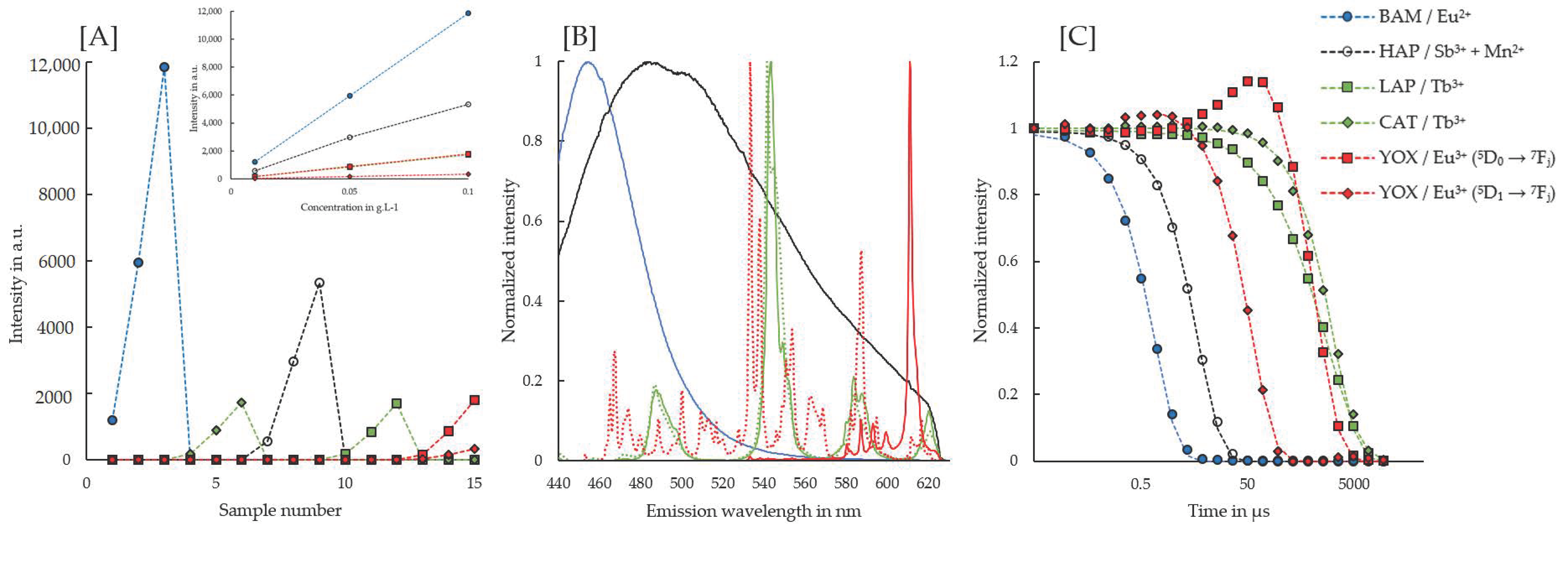
3.3. Time-Resolved Laser-Induced Fluorescence Spectroscopy

Of the REEs present in the investigated phosphors, cerium, terbium and europium are optically active due to the presence of 4f electrons and yttrium and lanthanum are optically inactive due their absence [29]. In LAP and CAT, Ce³⁺ functions as a sensitizing ion, absorbing incident photons and transferring the energy to Tb³⁺, which is the activator ion and emits green photons. In YOX and BAM, Eu³⁺ and Eu²⁺ are the activator ions, respectively emitting red and blue photons. The non-REE phosphor HAP has a broad emission spectrum, due to the complementary emission of blue light by Sb³⁺ and yellow light by Mn²⁺ [30].

A deconvolution of the phosphors’ emission spectra by PARAFAC requires trilinearity of components [24]. More specifically, in the case of our TRLFS setup, this means that each PARAFAC component must have a unique distribution within the (1) sample series, (2) emission spectrum and (3) luminescence decay. For the investigated system of five phosphors, this requirement is fulfilled with a six component PARAFAC model, as shown in Figure 2. The reason for the additional component is that the emission by Eu³⁺ in YOX had to be deconvoluted into two components. The main emission is composed of ⁵D₀ → ⁷F_j transitions, whereas an additional emission from the ⁵D₁ excited state is also detectable and results in a blue shifted spectrum with significant shorter lifetimes, as compared to the ⁵D₀ transitions. To fulfill the requirement of trilinearity, this emission had to be considered to be a separate PARAFAC component, but one that behaves synchronously to the main emission. Given this synchronous behavior, the two PARAFAC components for YOX were summed to a single distribution for the quantification of YOX in all our further work.

To account for differences in the luminescence lifetimes of the different phosphors over multiple orders of magnitude, we used an exponentially increasing stepsize in our TRLFS study. As shown in Figure 2C, the shortest emission lifetimes of approximately 0.9 μs and 6 μs were found for BAM and HAP, respectively. In YOX, the ⁵D₁ → ⁷F_j transition has a lifetime of about 60 μs, whereas the main ⁵D₀ → ⁷F_j transition has a longer emission lifetime of approximately 1 ms. The terbium containing phosphors emit light over a relatively long period of about 1.5 to 2.1 ms after excitation. The emission lifetimes of all phosphors but LAP could be well fitted with a mono-exponential decay. Interestingly, LAP is the only phosphor, whose decay follows a Kohlrausch function, i.e., a stretched exponential function. This is indicative for a superposition of several slightly different micro environments of Tb³⁺ [31,32]. Finally, it should be noted that the emission spectra (cf. Figure 2B) and emission lifetimes (cf. Figure 2C) of Tb³⁺ in LAP and CAT differ sufficiently for an accurate deconvolution.

The potential use of TRLFS with PARAFAC for deconvolution of mixed phosphor samples is validated in Supportive Information 1 by analysis of 13 mixed samples with randomly predetermined concentrations of each phosphor. The concentrations of these samples are presented in Table S1. In PARAFAC, these samples were analyzed together with the standard curve samples. Thus, the emission spectra and luminescence decays were the same as the ones shown in Figure 2. Furthermore, the distributions from the distinct YOX emissions (⁵D₀ → ⁷F_j and ⁵D₁ → ⁷F_j) were summed up for simplification. The results of the PARAFAC analysis performed on the TRLFS measurements of the synthetic mixtures are given in Figure S1. The deconvolution of the TRLFS data using PARAFAC worked excellently to obtain a linear correlation between the phosphors’ concentrations and the intensities of their PARAFAC components. Therefore, the approach to combine TRLFS with PARAFAC for phosphor quantification is validated.

3.4. High-Gradient Magnetic Separation

Figure 3A shows the evolution of each phosphors’ concentration during the removal stage within the HGMS experiments, whereas the removed and recovered fractions of each phosphor at the end of the experiment are depicted in Figure 3B. The concentrations in Figure 3A are shown as relative concentrations (RC), calculated from the TRLFS measurements according to the following equation:

$$R{C}^{\mathrm{phosphor}\mathrm{x}}\left(t\right)=\frac{I_{\mathrm{TRLFS}}^{\mathrm{phosphor}\mathrm{x}}\left(t\right)}{I_{\mathrm{TRLFS}}^{\mathrm{phosphor}\mathrm{x}}\left(t_0\right)}$$

(3)

where “phosphor x” represents one of the five investigated phosphors, t₀ is the experiments’ starting point and t is the time between t₀ and the moment of sampling.

It is clear from Figure 3A that the terbium-doped green phosphors LAP and CAT, which have the highest magnetic susceptibilities (cf. Table 2) were removed faster than the europium-doped blue phosphor BAM and red phosphor YOX. The white phosphor HAP, which does not contain any REEs and has the lowest magnetic susceptibility was removed the slowest. As most of the LAP and CAT were removed during the first 10 min of the experiment, it was decided to take a sample during every minute in this early phase. As shown in the figure, the phosphors’ RCs in this early phase can be well described by an exponential function. After this early phase, the removal dynamics of all phosphors decreased as seen in the deviations from the exponential fit. Nevertheless, 94.4 ± 0.6% of CAT and 92.0 ± 0.1% of LAP were removed during the experiment. At this point, approximately 70% of BAM and 60% of YOX and HAP were removed as well. Moreover, the RCs of all phosphors continued to decrease until the point that the device was switched to the “field off” mode, indicating that the removal of the phosphors was limited by the experiment’s duration. For comparison, the evolution of the phosphors’ RCs in the control experiments with the HGMS in the “field off” mode are presented in Figure S4.

After the device had been switched to the “field off” mode, the recoverability of the phosphors from the separation cell into a separate beaker was investigated in two steps. Assuming that for each phosphor the concentration in the initial beaker equaled the concentration in the loop volume (i.e., the separation cell and the tube system), it should be kept in mind that the total recoverable fraction in the second beaker consists of the removed fraction and the fraction in the loop volume. It is clear from Figure 3B that the first step, in which water was pumped through the separation cell in a downward direction at a high flow rate, is suboptimal for a recovery of the phosphors. In the second step, the application of an intermittent air–water flow was investigated, which facilitated a complete recovery of the removed phosphors. These results are in line with the findings of Kampeis et al., who have investigated multiple techniques for the recovery of superparamagnetic beads from a stainless steel wire mesh in the HGF-10 device [33].

4. Discussion

4.1. Magnetophoretic Velocity and High-Gradient Magnetic Separation

The magnetic or Kelvin force acting on a particle is given by the equation [26] (pp. 5–6):

$${\overrightarrow{F}}_{\mathrm{m}}=V·\frac{\chi }{{\mu }_0}(\overrightarrow{B}·\nabla )\overrightarrow{B}$$

(4)

where V and χ stand for the particle’s volume and volumetric magnetic susceptibility, respectively, $\overrightarrow{B}$ and $\nabla \overrightarrow{B}$ represent the magnetic field and its gradient, respectively, and μ₀ is the vacuum permeability.

Suspended particles with a relative motion with respect to the surrounding fluid undergo a counteracting viscous drag. The equation for the Stokes drag on spherical particles in a laminar flow regime is given by [34]:

$${\overrightarrow{F}}_{\mathrm{d}}=-3\pi d\eta \overrightarrow{v}$$

(5)

where d, η and $\overrightarrow{v}$ respectively represent the particle’s diameter, the dynamic viscosity of the surrounding fluid and the particle’s velocity relative to the fluid.

In the steady state, in which the Kelvin force, Equation (4), is balanced by the drag, Equation (5), a spherical particle moves with the magnetophoretic velocity:

$${\overrightarrow{v}}_{\mathrm{m}}=\frac{d^2}{18·\eta }·\frac{\chi }{{\mu }_0}·(\overrightarrow{B}\nabla )\overrightarrow{B}$$

(6)

which depends on both the physical properties of the particle (d, $\chi$) and the surrounding fluid ($\eta$), and on the magnetic field and its gradient. Although in low-gradient magnetic separation, the field gradient is generally less than 100 T·m⁻¹, the field gradient in high-gradient magnetic separation can be increased to thousands of T·m⁻¹ by introducing a magnetizable matrix (such as a steel wire mesh, steel balls, grooved plates or steel wool) into the magnetic field [25,35], as indicated in Figure 1.

4.2. Elucidation of the Empirically Observed Removal Dynamics

Based on the linear correlation between the phosphors’ concentrations and the intensities of their PARAFAC components, obtained with a combination of TRLFS and PARAFAC, we were able to quantify many samples to monitor each phosphors’ removal in the investigated HGMS. As shown in Figure 3A, the concentration of each phosphor decreased exponentially during the first 10 min of the experiment, according to the function e^−k·t. This finding indicates that in this early phase, a constant fraction of each phosphor was removed in the HGMS during each cycle in which the suspension was pumped through the separation cell. With cycle, we refer to the time required to pump the total volume through the separation cell. Hence a removal efficiency during a single cycle can be calculated according to the following equation:

$$\mathrm{Removal}\mathrm{Efficiency}=1-{\mathrm{e}}^{\frac{V_{\mathrm{tot}}}{Q}\mathrm{k}}$$

(7)

where V_tot and Q stand for the total volume of the suspension and the flow rate, respectively, and k represents the exponential constant in the evolution of the phosphors’ RCs as shown in Figure 3A. The exponential constants and the coefficients of determination for the exponential regressions of the early phase removal, as well as the calculated removal efficiencies for a V_tot of 1.5 L and a Q of 1000 mL·min⁻¹ are given in

Table 3. Exponential constant, k, and coefficient of determination, R², of the early phase removal with the associated removal efficiency of each phosphor.

Variable	LAP	CAT	BAM	YOX	HAP 1
k/min−1	0.123	0.123	0.057	0.041	0.039
R2	0.9886	0.9926	0.9766	0.9718	0.9093
Removal Efficiency	17%	17%	8%	6%	6%

¹ The relatively low coefficient of determination of the exponential fit to the removal of HAP could be attributable to the phosphor’s relatively broad PSD, low magnetic susceptibility, and/or low sphericity, as compared to the REE containing phosphors (cf. Table 2).

for each phosphor.

As the phosphor removal in the control experiments with the HGMS in the “field off” mode was inferior as compared to the removal shown in Figure 3A and was not clearly distinguishable for the different phosphors (cf. Supportive Information 2), we assume that phosphor removal in the HGMS was predominantly driven by magnetic capture on the wire matrix. In the context of a particle’s magnetic capture, a particle’s capture radius ($R_c$) is defined as the critical distance of the particle’s streamline to the wire’s stagnation streamline for the particle to be captured on the wire. Early works focused on the magnetic capture in an HGMS have described that a particle’s $R_c$ is proportional to the particle’s magnetic capture efficiency and, under the conditions investigated in this study, approximately proportional to ${\left(\frac{v_m}{v_0}\right)}^{1/3}$, with v₀ referring to the average cross sectional fluid velocity [36,37]. According to Equation (6), v_m is proportional to the particle-dependent component d²·χ, whereas v₀ can be considered to be a constant in this study. Hence, the relationship R_c ~ (d²·χ)^1/3 is obtained. It is interesting to note that this corresponds well with v_m ~ $d^2·\chi$·($B$·∇)B (Equation (6)), given the considerations that on a line perpendicular to the wire surface and longitudinal to the background field, ∇ B ~ $\frac{1}{r^3}$ and the approximation B ≈ B₀ holds with increasing distance to the surface (cf. Section 2.5). Furthermore, it is clear that for each phosphor, larger particles are removed faster than smaller particles. We propose that this preferential removal of larger particles may have caused a shift in the suspended phosphors’ PSDs during the HGMS experiment. Given the low loading rate in the investigated setup, we expect that it is the aforementioned shift in the PSDs that caused the decreasing removal dynamics after the first 10 min of the experiment, shown in Figure 3A, rather than a substantial saturation of the particles on the wire matrix. Nevertheless, the constant removal efficiencies during the first 10 min of the experiment indicate that in this early phase, the phosphors’ removal dynamics resembled those of monodisperse particles. Hence, the calculated removal efficiencies, presented in Table 3, can be related to the phosphors’ characterized properties, presented in Table 2, by the relationship Removal Efficiency ~ (d₅₀²·χ)^1/3, as shown in Figure 4.

4.3. Compensation Demanding Role of Broad Particle Size Distributions

It is clear from Table 1 and Table 2 that in an inter-phosphor comparison, the phosphors’ magnetic susceptibilities vary strongly, associated with their terbium and europium content. It is interesting to note that the latter two elements are also the fluorescent activator ions in the REE-doped phosphors, hereby determining the particles’ emission spectra, as discussed under Section 3.3. Hence, there is a direct link between the particles’ functional property, i.e., fluorescence, and a separation-facilitating property, i.e., magnetizability. However, although it can be assumed that each phosphor has a specific value for χ, in an intra-phosphor comparison, the particle-dependent components of the magnetophoretic velocity can widely vary, according to the phosphors’ broad PSDs. This causes large overlaps in the particle-dependent component of the Kelvin force acting on the different phosphors, as shown in Figure 5. Therefore, an efficacious separation of the phosphors cannot be implemented solely based on Kelvin forces despite the clear differences in the phosphors’ removal dynamics, e.g., a separation solely based on Kelvin forces of BAM and LAP, even with a cascade process, cannot result in a high purity and recovery simultaneously, as in each point in a magnetic field, large BAM particles have higher magnetophoretic velocities than small LAP particles. Hence, it can be expected that a shift in the recovered phosphors’ PSDs would detrimentally decrease the selectivity of subsequent separation steps in a cascade process.

The previously described problem was ingeniously solved by Yamashita et al. by separating fluorescent lamp phosphors in an HGMS through a simultaneous use of magnetic attraction and sedimentation [13,14,15]. This was done using an electromagnet-based HGMS with vertical magnetic field gradients. The magnitude of the field gradients was carefully chosen in order that the Kelvin force exerted on the more magnetizable phosphor LAP dominated over the gravitational force, whereas it was the other way around for the other phosphors. By repeatedly turning the field of the electromagnet on and off for periods of 15 s, it can be assumed that although e.g., larger BAM particles were attracted to the matrix faster than small LAP particles when the field was on, they were overall removed from LAP due to a faster sedimentation in the absence of the magnetic field. Hence, it can be said that the higher sedimentation velocities of larger particles compensated for the overlap of the magnetophoretic velocity’s particle-dependent component shown in Figure 5B. On the contrary to the HGMS device used by Yamashita et al., the HGF-10 has a horizontal magnetic field and captures paramagnetic particles horizontally, as shown in Figure 1A. Therefore, in the current configuration, the investigated device is not suitable for an efficacious phosphor separation based on a simultaneous use of magnetic and gravitational forces.

Finally, the recovery of CAT was outside the scope of Yamashita et al., as CAT is not commonly used in Japan. To the best of our knowledge, this is the first work focused on the separation of CFL phosphors by HGMS that included CAT. Although the terbium content and the magnetic susceptibility of CAT are about half of LAP, according to our findings CAT and LAP both had an initial removal efficiency of 17% (cf. Table 3) and had very similar recovery rates throughout the entire HGMS experiment (cf. Figure 3A). The proposed explanation for this finding is that in the size distributions, CAT has significantly larger particles than LAP, compensating for the magnetic susceptibility in the magnetophoretic velocity’s particle-dependent component, as shown in Figure 5.

4.4. Potential of the HGF-10 for a Peptide-Based Magnetic Phosphor Separation

As opposed to the HGMS presented by Yamashita et al. [13,14,15], the investigated configuration had a horizontal instead of a vertical field gradient and is not suitable for obtaining high-purity phosphors (cf. Section 4.3). Nevertheless, our findings can have important implications for a future separation of the phosphors with the HGF-10 by means of selectively surface-binding peptide functionalized superparamagnetic carriers.

In this work, it is for the first time that we investigate an HGF-10 for the separation of larger inorganic particles with relatively low magnetic susceptibilities. Previous studies with the device have focused on applications with superparamagnetic micron-sized composite beads and nanoparticles for the separation of target biomolecules from a fermentation broth [38], the recovery of biocatalysts [39], and fluoride removal from wastewater [40]. In these works, the HGF-10 was applied as a magnetic filter, effectively capturing close to 100% of the target particles during a single cycle through the separation cell until a filter breakthrough was observed, at which point the device was to be switched to the “field off” mode to allow for a recovery of the target particles.

By functionalizing superparamagnetic beads or nanoparticles with phosphor binding peptides identified by Lederer et al., target phosphors could be fished out of a mixed suspension, similarly to the HGF-10’s previous applications [16]. Although the general concept of particle separation by means of selectively surface-binding peptide functionalized superparamagnetic carriers has previously been demonstrated on a milliliter scale [18,19,20], to the best of our knowledge, its upscalability has yet to be proven. In this context, this work can be considered to be an important preparation of a future proof of the concept’s upscalability in the HGF-10. First, the high reproducibility of the HGMS experiment in this work indicates the solidity of both the setup of the HGF-10 and the phosphor quantification method, which can be used for future experiments. Secondly, although the current configuration is not suitable for as a separation method, it is clear that captured phosphors can effectively be held on the matrix in the separation cell, despite their low magnetic susceptibilities. Moreover, we have shown that a simple backwashing step with an intermittent air–water flow can recover nearly all the captured phosphors from the cell. However, we have also shown that in the current setup, a fraction of between 6% and 17% of each phosphor is captured on the wires during a single cycle through the cell. Therefore, we suggest that a peptide-based separation aiming at a high phosphor purity should be performed as a cascade process with multiple steps of separation in and recovery from the cell.

5. Conclusions

In summary, we have characterized five CFL phosphors in terms of their chemical compositions and physical properties that are most relevant for a magnetic separation (i.e., PSD, ρ, S_m, ψ and χ). Furthermore, we have characterized the phosphors’ luminescence emissions by a combination of TRLFS with PARAFAC. We have found that the trilinearity requirement is fulfilled for distribution within the (1) sample series, (2) emission spectrum and 3) luminescence decay with a six component PARAFAC model. By deconvolution of the TRLFS data with PARAFAC, linear correlations between the phosphors’ concentrations and the intensities of their PARAFAC components were obtained. Hence, we were able to quantify a large number of samples to monitor each phosphors’ removal in the investigated HGMS.

We have found that the phosphor concentrations in the HGMS decreased exponentially during the first 10 min of the experiment, after which the removal dynamics started to decrease. At the end of the experiment, we have found that the removed particles could be recovered very well from the separation cell by backwashing with an intermittent air–water flow. From an exponential regression analysis to the early phase removal, as well as from theoretical calculations of the field around a single wire in the investigated HGMS, we could obtain the relationship: Removal Efficiency ~ (d²·χ)^1/3, which is consistent with previous works on the magnetic capture efficiency in HGMS [36,37]. We have proposed that the preferential removal of larger particles of each phosphor may have caused a shift in the PSDs during the removal experiment, which could be the main cause of the decreasing removal dynamics throughout the experiment. Furthermore, we have stated that a combination of a PSD shift due to the preferential capture of large particles and the broad and overlapping PSDs, would hinder an efficacious separation of the phosphors with the device in the current configuration. Therefore, we conclude that the currently investigated process is not suitable as a separation method of CFL phosphors, but may be considered to be an important preparation for their separation, using superparamagnetic carriers, in the device initially designed for biotechnological separation purposes.

References

1. Binnemans, K.; Jones, P.; Blanpain, B.; Van Gerven, T.; Yang, Y.; Walton, A.; Buchert, M. Recycling of Rare Earths a Critical Review. J. Clean. Prod. 2013, 51, 1–22. [Google Scholar] [CrossRef]
2. Lee, J. Rare Earths from Mines to Metals: Comparing Environmental Impacts from China’s Main Production Pathways: Environmental Impacts of Rare Earths in China. J. Ind. Ecol. 2016, 21, 1277–1290. [Google Scholar] [CrossRef]
3. European Commission. Study on the EU’s List of Critical Raw Materials—Final Report (2020); European Commission: Brussels, Belgium, 2020. [Google Scholar]
4. Binnemans, K.; Jones, P. Perspectives for the recovery of rare earths from end-of-life fluorescent lamps. J. Rare Earths 2014, 32, 195–200. [Google Scholar] [CrossRef] [Green Version]
5. Dupont, D.; Binnemans, K. Rare-earth recycling using a functionalized ionic liquid for the selective dissolution and revalorization of Y2O3:Eu3+ from lamp phosphor waste. Green Chem. 2015, 17, 856–868. [Google Scholar] [CrossRef] [Green Version]
6. Hopfe, S.; Flemming, K.; Lehmann, F.; Möckel, R.; Kutschke, S.; Pollmann, K. Leaching of rare earth elements from fluorescent powder using the tea fungus Kombucha. Waste Manag. 2017, 62, 211–221. [Google Scholar] [CrossRef] [PubMed]
7. Takahashi, T.; Takano, A.; Saitoh, T.; Nagano, N.; Hirai, S.; Shimakage, K. Separation and Recovery of Rare Earth Elements from Phosphor Sludge in Processing Plant of Waste Fluorescent Lamp by Pneumatic Classification and Sulfuric Acidic Leaching. Shigen-to-Sozai 2001, 117, 579–585. [Google Scholar] [CrossRef] [Green Version]
8. Hirajima, T.; Sasaki, K.; Abel, B.; Hirai, H.; Hamada, M.; Tsunekawa, M. Feasibility of an efficient recovery of rare earth-activated phosphors from waste fluorescent lamps through dense-medium centrifugation. Sep. Purif. Technol. 2005, 44, 197–204. [Google Scholar] [CrossRef]
9. Hirajima, T.; Abel, B.; Sasaki, K.; Nakayama, K.; Hirai, H.; Tsunekawa, M. Floatability of rare earth phosphors from waste fluorescent lamps. Int. J. Miner. Process. 2005, 77, 187–198. [Google Scholar] [CrossRef]
10. Otsuki, A.; Dodbiba, G.; Shibayama, A.; Sadaki, J.; Mei, G.; Fujita, T. Separation of Rare Earth Fluorescent Powders by Two-Liquid Flotation using Organic Solvents. Jpn. J. Appl. Phys. 2008, 47, 5093–5099. [Google Scholar] [CrossRef]
11. Mei, G.; Rao, P.; Mitsuaki, M.; Fujita, T. Separation of red (Y2O3: Eu3+), blue (Sr, Ca, Ba)10(PO4)6Cl2: Eu2+ and green (LaPO4: Tb3+, Ce3+) rare earth phosphors by liquid/liquid extraction. J. Wuhan Univ. Technol. Mater. Sci. Ed. 2009, 24, 418–423. [Google Scholar] [CrossRef]
12. Wada, K.; Mishima, F.; Akiyama, Y.; Nishijima, S. The Development of the Separation Apparatus of Phosphor by Controlling the Magnetic Force. Phys. Procedia 2014, 58, 252–255. [Google Scholar] [CrossRef] [Green Version]
13. Yamashita, M.; Akai, T.; Imamura, T.; Murakami, M.; Oki, T. Recycling of waste phosphors using high gradient magnetic separation method. Trans. Mater. Res. Soc. Jpn. 2014, 39, 35–37. [Google Scholar] [CrossRef] [Green Version]
14. Akai, T.; Ataka, M.; Yamashita, M. Recycling Method of Waste Phosphor. Japan Patent JP 5120963, 16 January 2013. [Google Scholar]
15. Yamashita, M.; Akai, T.; Murakami, M.; Oki, T. Recovery of LaPO4:Ce,Tb from waste phosphors using high-gradient magnetic separation. Waste Manag. 2018, 79, 164–168. [Google Scholar] [CrossRef]
16. Lederer, F.; Curtis, S.; Bachmann, S.; Dunbar, S.; MacGillivray, R. Identification of lanthanum-specific peptides for future recycling of rare earth elements from compact fluorescent lamps: Peptides for Rare Earth Recycling. Biotechnol. Bioeng. 2016, 114, 1016–1024. [Google Scholar] [CrossRef]
17. Pollmann, K.; Kutschke, S.; Matys, S.; Raff, J.; Hlawacek, G.; Lederer, F. Bio-recycling of metals: Recycling of technical products using biological applications. Biotechnol. Adv. 2018, 36, 1048–1062. [Google Scholar] [CrossRef] [PubMed]
18. Vreuls, C.; Genin, A.; Zocchi, G.; Boschini, F.; Cloots, R.; Gilbert, B.; Martial, J.; Weerdt, C. Genetically engineered polypeptides as a new tool for inorganic nano-particles separation in water based media. J. Mater. Chem. 2011, 21, 13841–13846. [Google Scholar] [CrossRef]
19. Essinger-Hileman, E.; Popczun, E.; Schaak, R. Magnetic separation of colloidal nanoparticle mixtures using a material specific peptide. Chem. Commun. 2013, 49, 5471. [Google Scholar] [CrossRef] [PubMed]
20. Cetinel, S.; Shen, W.-Z.; Aminpour, M.; Bhomkar, P.; Wang, F.; Borujeny, E.; Sharma, K.; Nayebi, N.; Montemagno, C. Biomining of MoS2 with Peptide-based Smart Biomaterials. Sci. Rep. 2018, 8, 3374. [Google Scholar] [CrossRef] [PubMed] [Green Version]
21. Hoffmann, C.; Franzreb, M.; Holl, W.H. A novel high-gradient magnetic separator (HGMS) design for biotech applications. IEEE Trans. Appl. Supercond. 2002, 12, 963–966. [Google Scholar] [CrossRef]
22. Andersson, C.A.; Bro, R. The N-way Toolbox for MATLAB. Chemom. Intell. Lab. Syst. 2000, 52, 1–4. [Google Scholar] [CrossRef]
23. Drobot, B.; Bauer, A.; Steudtner, R.; Tsushima, S.; Bok, F.; Patzschke, M.; Raff, J.; Brendler, V. Speciation Studies of Metals in Trace Concentrations: The Mononuclear Uranyl(VI) Hydroxo Complexes. Anal. Chem. 2016, 88, 3548–3555. [Google Scholar] [CrossRef] [PubMed]
24. Drobot, B.; Schmidt, M.; Mochizuki, Y.; Abe, T.; Okuwaki, K.; Brulfert, F.; Falke, S.; Samsonov, S.A.; Komeiji, Y.; Betzel, C.; et al. Cm3+/Eu3+ induced structural, mechanistic and functional implications for calmodulin. Phys. Chem. Chem. Phys. 2019, 21, 21213–21222. [Google Scholar] [CrossRef] [PubMed]
25. Ge, W.; Encinas, A.; Araujo, E.; Song, S. Magnetic matrices used in high gradient magnetic separation (HGMS): A review. Results Phys. 2017, 7, 4278–4286. [Google Scholar] [CrossRef]
26. Svoboda, J. Magnetic Techniques for the Treatment of Materials; Kluwer Academic Publishers: Dordrecht, The Netherlands, 2004. [Google Scholar]
27. Franzreb, M. Magnettechnologie in der Verfahrenstechnik Wässriger Medien; University of Karlsruhe: Karlsruhe, Germany, 2003. [Google Scholar]
28. Wadell, H. Volume, Shape, and Roundness of Quartz Particles. J. Geol. 1935, 43, 250–280. [Google Scholar] [CrossRef]
29. Tanaka, M.; Oki, T.; Koyama, K.; Narita, H.; Oishi, T. Recycling of rare earths from scrap. In Handbook on the Physics; and Chemistry of Rare Earths; Bunzli, J.C.G., Pecharsky, V.K., Eds.; Elsevier: Amsterdam, The Netherlands, 2013; Volume 43, pp. 159–211. [Google Scholar]
30. Srivastava, A.M.; Ronda, C.R. Phosphors. In The Electrochemical Society Interface; The Electrochemical Society, Inc.: Pennington, NJ, USA, 2003; Volume 12, p. 48. [Google Scholar]
31. Greben, M.; Khoroshyy, P.; Sychugov, I.; Valenta, J. Non-exponential decay kinetics: Correct assessment and description illustrated by slow luminescence of Si nanostructures. Appl. Spectrosc. Rev. 2019, 54, 758–801. [Google Scholar] [CrossRef]
32. Zatsepin, A.; Kuznetsova, Y. Kinetic selection of nonradiative excitation in photonic nanoparticles Gd2O3:Er. Phys. Chem. Chem. Phys. 2020, 22, 6818–6825. [Google Scholar] [CrossRef] [PubMed]
33. Kampeis, P.; Bewer, M.; Rogin, S. Einsatz von Magnetfiltern in der Bioverfahrenstechnik Teil 1: Vergleich Verschiedener Verfahren zum Rückspülen der Magnetfilter. Chem. Ing. Tech. 2009, 81, 275–281. [Google Scholar] [CrossRef]
34. Wills, B.; Napier-Munn, T. Mineral Processing Technology: An Introduction to the Practical Aspects of Ore Treatment and Mineral Recovery; Elsevier Science & Technology Books: Amsterdam, The Netherlands, 2006. [Google Scholar]
35. Leong, S.; Yeap, S.P.; Lim, J.K. Working principle and application of magnetic separation for biomedical diagnostic at high- and low-field gradients. Interface Focus 2016, 6, 20160048. [Google Scholar] [CrossRef] [Green Version]
36. Birss, R.; Dennis, B.; Gerber, R. Particle capture on the upstream and downstream side of wires in HGMS. IEEE Trans. Magn. 1979, 15, 1362–1363. [Google Scholar] [CrossRef]
37. Uchiyama, S.; Hayashi, K. Analytical Theory of Magnetic Particle Capture Process and Capture Radius in High Gradient Magnetic Separation. In Proceedings of the International Conference on Industrial Applications of Magnetic Separation, Rindge, NH, USA, 30 July–4 August 1978; p. 169. [Google Scholar]
38. Shaikh, Y.; Kampeis, P. Development of a novel disposable filter bag for separation of biomolecules with functionalized magnetic particles. Eng. Life Sci. 2017, 17, 817–828. [Google Scholar] [CrossRef] [Green Version]
39. Schultz Jensen, N.; Syldatk, C.; Franzreb, M.; Hobley, T. Integrated processing and multiple re-use of immobilised lipase by magnetic separation technology. J. Biotechnol. 2007, 132, 202–208. [Google Scholar] [CrossRef] [PubMed]
40. Chang, C.-F.; Chang, C.-Y.; Hsu, T.-L. Removal of fluoride from aqueous solution with the superparamagnetic zirconia material. Desalination 2011, 279, 375–382. [Google Scholar] [CrossRef]
Figure 1. (A) Distribution of the magnetic field around a 430 grade stainless steel wire with a diameter of 670 μm in a horizontal background field with an intensity of 0.32 T, simulated according to Equation (1), based on hysteresis loops reported by Franzreb, the saturation polarization was estimated at 1.5 T [27]. Due to the direction of the magnetic field gradient, the wire surface is attractive and repulsive to paramagnetic particles in the longitudinal and transversal direction, respectively. (B) Course of the magnetic field and its gradient on a line perpendicular to the wire surface and longitudinal to the background field with increasing distance to the wire surface.
Minerals 11 01116 g001
Figure 2. PARAFAC results of samples containing pure phosphors. Standard curves, containing concentrations of 0.01, 0.05 and 0.10 g·L−1 were measured for BAM (samples 1–3), CAT (samples 4–6), HAP (samples 7–9), LAP (samples 10–12) and YOX (samples 13–15), respectively. All samples were analyzed simultaneously with PARAFAC. (A) Distributions of the single PARAFAC components. For YOX, two components were needed to account for the different Eu3+ emittive levels, i.e., 5D0 and 5D1. The inset shows the linear correlation of the phosphors’ luminescence signal versus their concentrations. (B) Emission spectrum of each PARAFAC component. On this Figure, the same color code is used as shown in the legend and solid lines are used for LAP and the 5D07Fj transition of YOX, whereas dashed lines are used for CAT and 5D17Fj transition of YOX. (C) Luminescence decay of the PARAFAC components. The dashed lines represent the fits of the luminescence decays. The decay of LAP was fitted with a stretched exponential function, whereas the other decays were all fitted with a mono-exponential function.
Minerals 11 01116 g002
Figure 3. (A) Evolution of the phosphors’ RCs during the removal experiments with the HGMS. For each phosphor, an exponential regression (“Expon.”) of the type RC = e−k·t was fitted to the observations of the first 10 min. (B) Estimated phosphor fractions that were removed, with and without taking the loop volume into account, and recovered in a separate beaker after cleaning of the separation cell with water at a high flow rate and an intermittent air–water flow. The error bars depict one standard deviation.
Minerals 11 01116 g003
Figure 4. Correlation between the phosphors’ d 50 2 · χ 3 and the removal efficiencies presented in Table 3.
Minerals 11 01116 g004
Figure 5. (A) Cumulative volume weighted PSD of the phosphors, as determined by laser diffraction analysis. (B) Volume weighted PSD of the phosphors in function of the particle-dependent component of the magnetophoretic velocity.
Minerals 11 01116 g005