Abstract
In research on the particle–bubble collision process, due to the adsorption of surfactants and impurities (such as mineral particles, slime, etc.), most studies consider the bubble surface environment to be immobile. However, in the real situation of froth flotation, the nature of the bubble surface (degree of slip) is unknown. Mobile surface bubbles increase the critical thickness of the hydration film rupture between particles and bubbles, and enhance the collision between particles and bubbles. Sam (1996) showed that when the diameter of the bubble is large enough, a part of the surface of the bubble can be transformed into a mobile state. When the bubble rises in a surfactant solution, the surface pollutants are swept to the end of the bubble, so when the bubble reaches terminal velocity, the upper surface of the bubble is changed into a mobile surface. This paper analyzes the collision efficiency and fluid flow pattern of bubbles with mobile and immobile surfaces, and expounds the influence of surface properties on collision efficiency.
1. Introduction
A better understanding of controlling factors in mineral flotation is possible using advanced computational fluid dynamics (CFD) simulations of entire full-scale industrial cells. Such macro-scale simulations require sub-models to quantitatively describe the rates of bubble–particle attachment and detachment: the huge number of particles and bubbles in an industrial cell mean that macro-scale models cannot resolve the details of bubble–particle interaction [1] (see for example, Koh and Schwarz, 2006). Micro-scale models and experimental investigations can be used to improve sub-model formulas for attachment and detachment rates.
In the picture of the flotation phenomenon described by Mika and Fuerstenau [2], the process of the collision of a particle with a bubble is envisaged to occur as three subprocesses: bubble–particle collision; formation of a three-phase contact between particle and bubble resulting in a bond between the two; and stabilization against detachment. This conceptual model allows analysis of the kinetics of the process, by considering collision efficiency, (three-phase) attachment, and stabilization. This paper focuses on the first of these sub-processes, namely the bubble–particle collision.
There have been many different studies of the collision between a particle and a bubble. Most, until recently, have been theoretical or semi-theoretical. Experimental studies are difficult to carry out because of the difficulty of controlling the parameters of the collision, and, in the past, visualization has also been problematic. The advent of high-speed video, however, has overcome this latter problem.
A review of the development of the theoretical approach was undertaken by Li et al. [3]. That paper also detailed two of the best-known correlations arising from the theoretical development, namely those of Schulze (1989) [4] and Dukhin model [5]. As Schulze did, Dukhin also modify the Sutherland theory for the influence of the particle inertial force, and the resulting equations have been called the Generalized Sutherland Equation (GSE). As shown by Li et al. and others [3], these two formulations give quite different predictions for the bubble–particle collision efficiency. They carried out CFD simulations of the simple collision configuration treated by both the theoretical correlations, and showed that the Schulze model agreed much better with the simulation results.
Identification of each model is outlined with regard to the bubble surface mobility, fluid flow, and those sub-processes involved (i.e., interceptional, gravitational, and inertial effects) in Table 1 [6].

Table 1.
Hassanzadeh’s review of the main assumptions and drawbacks of different analytical and numerical models representing particle–bubble collision efficiency.
For the sake of simplicity and to facilitate a comparison with the theory, these CFD simulations neglected some effects that only become important near the bubble surface, which could be called near-field hydrodynamics effects. These include lubrication force, lift force, and modifications to the drag force. To these could be added the effect related to whether the bubble surface is mobile or immobile—adsorption of surfactants could render the bubble interface somewhat immobile, i.e., able to apply shear stress. In this paper, we address the impact of some of these near-field effects on bubble–particle collision efficiency by incorporating them into the CFD simulation.
This study is of importance, first, because Li et al. [7] identified differences between published theoretical correlations for collision efficiency and predictions from their CFD model, which attempted to replicate the idealized arrangement treated by the theories. It is of interest, therefore, to determine whether near-bubble hydrodynamic effects have any further influence on the predictions. Second, to extend the CFD model to investigate not only collision efficiency but also the sliding of the particles over the bubble surface, such near-bubble effects are likely to be important.
There have been a few studies in which particle trajectories have been calculated and in which near-bubble effects have been accounted for but, in most cases, the calculations were carried out for a mobile interface, and usually either no fluid flow was assumed, or a theoretical potential flow solution was used. In this work, we tackle the more general case with a fluid solver, which will predict exact flow velocities (within the tolerance of the calculations, and within the ideal assumptions, such as spherical bubble shape, spherical particle, etc.).
Verrelli et al. [7] calculated trajectories in the absence of any fluid flow because they compared them with measured trajectories for a stationary bubble. Because of the absence of flow, there were only minor differences between the mobile and immobile cases, though the particles fell away from the bubble slightly earlier in the mobile case. The near-bubble effects are, unsurprisingly, small at distances less than a particle diameter, but there appears to be some influence on computed trajectories at distances of three or four particle diameters from the bubble surface. The effects at these distances are not so apparent in the experimentally observed trajectories.
2. Theoretical Development
2.1. Schulze Model Theory
Schulze considers three different effects in the collision efficiency model—the interceptional effect, the gravity effect, and the inertia effect—and the total collision efficiency is the sum of these three collision efficiencies.
2.1.1. The Interceptional Effect
Schulze interpreted intercepting collisions as a collision effect that is purely due to the overlapping space of particles rather than relying on the mass of the particles.
Representing the value of the particle’s flow function that only passes through the bubble by ψc, and describing the terminal velocity of the particle, the flow function of the key streamline can be written as
The interceptional efficiency () is shown as
when Vp < Ub, the formula above can be simplified to
The stream-function
can be defined as
Schulze gives the stream function of the grazing trajectory under an immobile bubble surface as an approximate expression:
Notice that the provided particle is much smaller than the bubble.
2.1.2. The Gravitational Effect
Schulze [4] described collision efficiency with the gravity effect in the Weber–Paddock model [8], where the correction of the collision efficiency caused by gravity is as follows:
An important result of this movement of particles from the fluid streamlines is that the collision point of the critical grazing trajectory is moved forward to an angle θc < π/2, i.e., the particle collides with the bubble before it reaches the midplane of the bubble [9]. For inactive interfaces, the relationship between the critical collision angle θc (in degrees) and the bubble Reynolds number is approximately [6]:
For a mobile bubble, Weber and Paddock [8] gave an approximated angle θc of 90°. It is worth noting that Flint and Howarth [3] show that if the particles are sufficiently small that the interceptional effect can be neglected, for mobile interfaces the collision efficiency (which is only the gravitational effect in this case) is simply [10]
where
and Vp and Ub are the terminal velocity of the particle and bubble, respectively.
2.1.3. The Inertial Effect
The inertial effect illustrates the tendency of finite mass particles to continue to move in a straight line. The approximate correction term for the interception efficiency has been expressed as
where a and b are fitting constants that depend on the bubble Reynolds number, and K is the Stokes number, which is used to describe the inertia behavior of suspended particles in the fluid, and is given by the ratio of the particle inertia force to resistance:
where ρp is the particle density. In summary, Schulze gives the inertial collision efficiency as [11]
The total collision efficiency is the sum of the three terms above:
2.2. GSE Model Theory
Dukhin derived the angle, θt, in the GSE model according to the following Formula [5]:
The dimensionless number, β, can be defined as
where the parameter f is related to the surface fluidity of the bubble (f = 2 for a mobile interface according to Dai et al. [11]). The parameter K3, is related to the Stokes number:
Dai etc. [11] reported that starting with the basic particle trajectory equation (also known as the Bathet–Busenes–Ossen equation when including the Bathet force), Dukhin [5] derived an analytical expression for collision efficiency:
3. CFD-based Micro-Scale Modelling Method for Bubble-Particle Collision Efficiency
In order to explain the interaction between particles and bubbles in the flotation process, a CFD model is established in this paper (see Figure 1 and Figure 2 as reported by Li 2019 [3]). In this paper, we summarize the first step of the Sutherland–Schulze hypothesis by performing numerical calculations on fluid flow and particle trajectory, while retaining other assumptions. The CFD model can explain the errors involved in the analysis model in detail and bring in other environmental factors that affect particle–bubble collisions in subsequent work, such as turbulence, fluid viscosity, etc. Notice that this paper ignores the effects of bubble deformation.
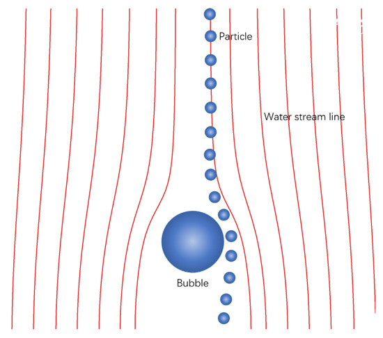
Figure 1.
Bubble–particle interaction process with water streamlines from computational fluid dynamics (CFD) simulation in a frame of reference in which the bubble is stationary (Li 2019) [3].
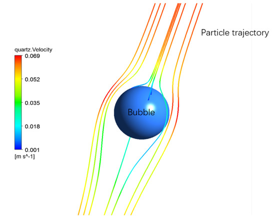
Figure 2.
3D schematic of typical particle paths around a bubble caused by relative motion between the bubble and surrounding slurry. The tendency of particles to follow streamlines, as illustrated, reduces the collision frequency below the straight path interception frequency (Li 2019) [3].
In this paper, a small volume near a single bubble is considered. In this case, the momentum equation and the mass conservation equation can be solved in the volume. The paper simulates a spherical bubble floating at a constant velocity by using a frame based on a fixed frame of reference. Moreover, in this frame, the pulp flows downwards and passes through fixed bubbles. Three-dimensional models can be built using the commercial CFD software package CFX19. The computational domain is a cylindrical region. In order to eliminate the influence of the region boundary, the computational domain is set sufficiently large. The dimensions are length × diameter = 0.04 m × 0.03 m. Table 2 shows the number of meshes, number of particles, Reynolds number, and fluid velocities corresponding to the bubble diameter example. The number of meshes is obtained through mesh-independence verification.
Table 2.
The mesh numbers, particle numbers, fluid velocities, and Reynolds number corresponding to the bubble diameter.
Under the assumptions of the paper, the collision of particles only occurs at the front of the bubble, and the particle injection area is shown in Figure 3. Thus, the collision efficiency should be the ratio between collision particles and total particles.

Figure 3.
Computational fluid mechanics model and particle tracking scheme for analyzing bubble-particle collisions.
The fluid flow is solved by standard laminar incompressible continuity and momentum equations:
∇(ρ) = 0
∇(ρμu) = −∇p + ∇µ ∇(u)
In the computational fluid dynamics model used in this paper, in order to analyze the collision efficiency and make a comparison with the semi-analytical model, the influence of liquid density and viscosity is ignored. The liquid viscosity is set as the ideal liquid condition, that is, the liquid density is 1000 kg/m3 and the liquid viscosity is 1 × 10⁻³ Pa·s. This assumption is also the same as the assumed fluid environment under the semi-analytic model.
At the bubble scale, the most important process is the collision of bubbles and particles. Then, based on these basic turbulence fields, and on basic physical principles and experimental measurements, formulas are used to predict the frequency and efficiency of local collisions [12]. In this paper, the effect of bubble deformation on particle capture is ignored. The surface of the bubble is set as a free sliding wall, which means that the surface of the bubble is assumed to be a movable surface.
In this paper, the particle trajectory is calculated using the Lagrangian method (particles are calculated as mass points under the Lagrangian algorithm). The change in particle diameter only affects the resistance equation and the mass equation. The Lagrangian method is based on using Newton’s second law to solve the momentum equation in order to calculate the motion trajectory of each particle. The calculation formula is
The particles are captured by the bubbles after colliding with them. The collision criterion is that the center of the particle collides with the surface of the bubble. The momentum transfer between fluid and particles is mainly transmitted through the resistance between phases. However, in this paper, the interaction method between particles and carrier liquid is the one-way coupling method; that is, the force of particles on the fluid term is ignored, so the resistance is the resistance of the fluid to the particles. The current paper considers drag, buoyancy, pressure, and additional mass forces, so the term on the right side of Formula (20) can be expressed as
where FD is the drag force, and FG, FP and FA are gravitational force, pressure gradient force, and added mass force, respectively:
where Rp is the radius of the particle, p is the pressure in the fluid phase, ρ and ρp are the density of the fluid and particles, and u and vi are the velocity of the fluid and particles, respectively. The derivative of fluid velocity is the total derivative with particle motion. It is worth noting that the variables u and vi used earlier in this paper are functions of position and time, and are different from the velocities of particles and bubbles, ub and vp.
4. Results and Discussion
4.1. Effects of Bubble Surface Properties on Bubble Near-Wall Flow Field
As can be seen from Figure 4 and Figure 5, the surface properties of the bubbles have a greater effect on the fluid flow regime in the bubble surface area. For immobile bubbles, the fluid velocity around the bubbles is lower. However, the area farther from the bubble on both sides of the bubble still has a larger fluid velocity area, and the wake turbulence is severe. The velocity of the fluid near the sides of the sliding surface bubble is significantly higher than that of the immobile surface fluid. The high velocity area is larger, the fluid deceleration area above the bubble is smaller, and the tail turbulence is not obvious.
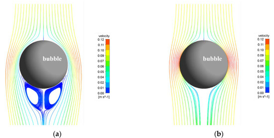
Figure 4.
Water streamline at bubble diameter = 0.9 mm (a) immobile surface bubble; (b) mobile surface bubble.
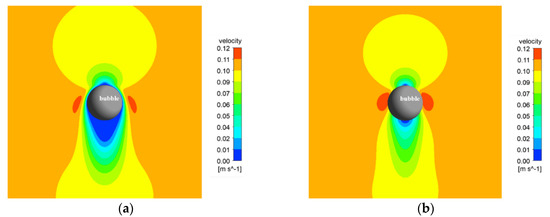
Figure 5.
Water velocity contour at bubble diameter = 0.9 mm (a) immobile surface bubble; (b) mobile surface bubble.
Due to the large fluid velocity in the area on both sides of the bubble under mobile surface conditions, the centrifugal negative inertia effect is larger when the particles move into this area. The collision efficiency caused by this part effect should be lower than that under the conditions of an immobile bubble surface. However, under immobile bubble surface conditions, the fluid deceleration area in the area above the bubble is larger, and the positive effect of the collision efficiency caused by the inertial effect of the particles approaching the bubble is reduced. The particles break through the hydrated film on the surface of the bubble and collide with the bubble. The tendency is lower than the collision efficiency under mobile bubble surface conditions.
Figure 6 shows the pressure contour of the mobile and immobile bubble surface bubbles. Similar to the velocity contour, the pressure contour also shows that no matter the bubble surface conditions, there is a negative pressure area on both sides of the bubble. However, the negative pressure area of the immobile surface bubble is smaller than that of the mobile surface, and there is no negative pressure area at the tail. Theoretically, the negative pressure region is conducive to the particles moving towards the surface of the bubble, thereby causing a collision phenomenon. To sum up, the collision efficiencies under mobile and immobile surface bubbles both depend on the overall effect of the above factors.
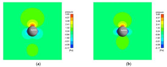
Figure 6.
Water pressure contour at bubble diameter = 0.9 mm. (a) immobile surface bubble; (b) mobile surface bubble.
4.2. Effects of Bubble Surface Properties on Particle-Bubble Relative Motion Behavior
Figure 7 and Figure 8 show the comparison of the particle motion trajectory and fluid streamlines under the conditions that the bubble diameter is 0.9 mm and the mineral particles are galena (density is 7500 kg/m3). Figure 8 is a partially enlarged view of Figure 7; the black lines are particle trajectories around the bubble. Figure 8a shows the comparison of particle motion trajectory and fluid streamlines without a mobile surface bubble; Figure 7b, Figure 8b show the particle trajectory with fluid streamlines under a mobile surface bubble. It can be seen from this set of figures that the fluid at the surface of the bubble on the sliding surface has a higher velocity at the position of the bubble surface than the fluid under the conditions of an immobile surface bubble. At the same time, the particle trajectory shows that under the conditions of a mobile surface bubble, the particles are closer to the bubble surface at a larger fluid velocity. However, when approaching the surface of the bubble, due to the greater centrifugal (negative) inertial effect caused by a larger velocity, the particles slide along the tangent direction of the surface of the bubble and move away from the bubble. Under this particular condition, the particles did not collide with the bubbles.
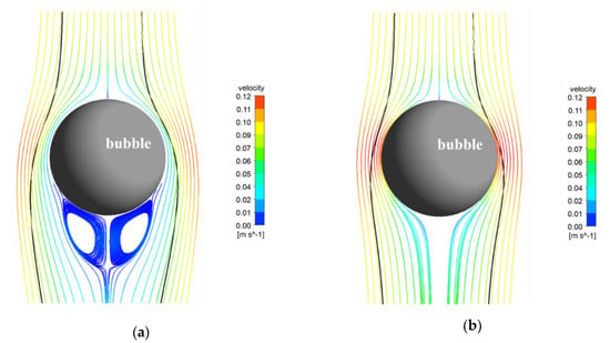
Figure 7.
Particle tracks and mean streamlines for bubble diameter of 0.9 mm and galena particle diameter of 150 μm (a) immobile surface; (b) mobile surface.
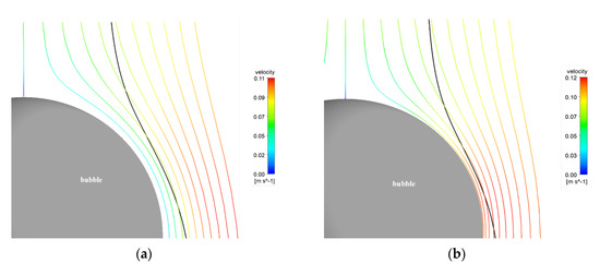
Figure 8.
Particle tracks and mean streamlines for bubble diameter of 0.9 mm and galena particle diameter of 150 μm (a), immobile surface; (b), mobile surface.
The results shown in Figure 9 are the same as the particle’s motion process described above. When the particles are close to the bubble region, the velocity is affected by the interception effect, and the particles begin to shift under the effect of centrifugal force. At the same time, under the effect of centrifugal inertia, the particles began to accelerate. Under this process, the particles are closer to the bubble surface under mobile surface conditions, and the particle velocity affected by the fluid velocity is also greater than the particle velocity under the immobile surface bubble.
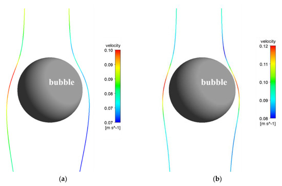
Figure 9.
Particle tracks with velocity for bubble diameter of 0.9 mm and galena particle diameter of 150 μm (a) immobile surface; (b) mobile surface.
4.3. Particle-Bubble Collision Efficiencies under Mobile and Immobile Bubble Surface Conditions
Figure 10 shows the comparison of collision efficiency between the Schulze model, the GSE model, and the CFD model under the conditions of a mobile surface bubble. Particle diameter of 74 μm, bubble diameter of 0.9 mm, and particle density of 4200 kg/m3 are used as condition criteria. Figure 10 shows (a) the influence of the bubble diameter on collision efficiency; (b) the influence of particle density on collision efficiency; and (c) the influence of particle diameter on collision efficiency.
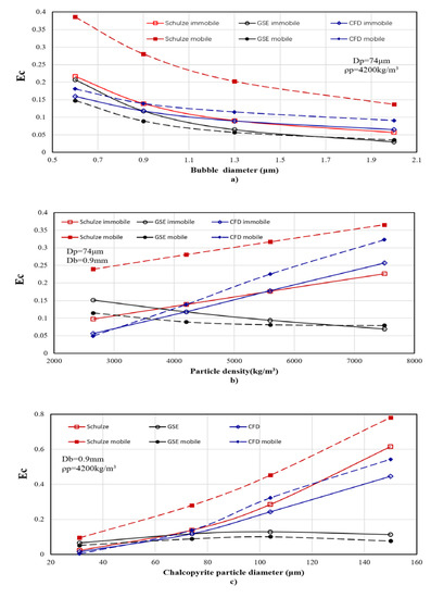
Figure 10.
Comparison of the effect of (a) bubble diameter (Db), (b) particle density (ρp), and (c) particle diameter (Dp) respectively, on Schulze, GSE, and CFD predictions for collision efficiency.
As shown in Figure 10a, the collision efficiency in all three models decreases with the bubble diameter increasing. At the same time, in the Schulze and CFD models, the collision efficiency under immobile surface bubbles is lower than under the mobile surface bubble conditions. In addition, the collision efficiency under the two conditions changes in proportion. However, under the Schulze model, the difference in collision efficiency between the two conditions is significantly greater, while the GSE model shows the opposite trend. That is, the collision efficiency is higher under the immobile bubble surface. This is because the centrifugal (negative) inertia effect under the bubble conditions on the mobile surface is larger, and the GSE model overcalculates the centrifugal (negative) inertia effect.
The Schulze model and CFD results have the same trend in the change of collision efficiency caused by particle density, but the GSE model shows the opposite results.
The Schulze and CFD model results show lower collision efficiency under immobile surface bubble conditions than under mobile surface bubble conditions. It is worth noting that the CFD results show collision efficiency for the mobile surface is larger than for the immobile surface with low particle density. The reason for this phenomenon may be that the fluid velocity above the surface of the mobile surface bubble is larger than that of the immobile surface bubble, so that at small particle mass, the inertial efficiency is smaller, and a small particle means the centrifugal negative inertia effect produced by the smaller particle is relatively large. As noted above, the collision efficiency in the immobile surface condition is lower.
Differently from the two model results above, the GSE model shows that collision efficiency decreases as particle density increases, and the rate at which collision efficiency decreases for the immobile surface bubble is larger than that for the mobile surface bubble. When particle density is small, the GSE model results in a mobile surface collision efficiency that is larger than the immobile surface collision efficiency. However, when the particle density is large, the opposite is shown. This may be because the value of the centrifugal (negative) inertial effect in the GSE model slowly increases to flatten as the particle density increases, while the inertial effect gradually increases. This can also explain that, under the conditions of a mobile surface bubble, when the particle density increases to a certain extent, the collision efficiency tends to increase slightly.
Figure 10a shows that the impact of the particle diameter on collision efficiency is similar to that of the particle density. The Schulze model results are consistent with those of the CFD model. Under the condition of a larger particle diameter, the results of the CFD model are slightly lower. In the Schulze and CFD models, the collision efficiency under an immobile surface bubble is lower than that under a mobile surface bubble. In the Schulze model, the collision efficiency under the two bubble surface conditions increases proportionally. This is because, when the Schulze model changes the properties of the bubble surface, it only has a positive gain on the gravity effect and inertial effect caused by changing the fluid velocity on the bubble surface, without taking into account the negative gain of the centrifugal effect. In computational fluid dynamics, several factors are considered at the same time. Therefore, when the particle diameter is small, the centrifugal (negative) inertial effect of the particle is obvious. As an example, when the particle diameter is 31 μm, the collision efficiency under the conditions of an immobile surface bubble is larger than that under the conditions of a mobile bubble surface. With the increase of particle diameter, the increase of the gravity effect and inertia effect of particles under the conditions of a mobile bubble surface gradually becomes larger than the centrifugal (negative) inertia effect, and the collision efficiency increases, which is greater than that under immobile surface conditions.
Similarly, the effect of the particle diameter on the collision efficiency of the GSE model is opposite to that of the other two models. When the particle diameter is larger than 74 μm, the collision efficiency decreases with the increase of particle diameter. At the same time, the collision efficiency of the GSE model under mobile and immobile bubble surface conditions varies proportionally. Unlike the other two models, the collision efficiency of the GSE model under the conditions of a mobile surface bubble is lower than that of the immobile surface bubble.
Figure 11 shows the relationship between Schulze, GSE, and CFD simulation models for collision efficiency for bubble diameters of 0.6 mm (a,b) and 1.3 mm (c,d), and particle densities of 2650 kg/m3 (a,c) and 5600 kg/m3 (b,d).
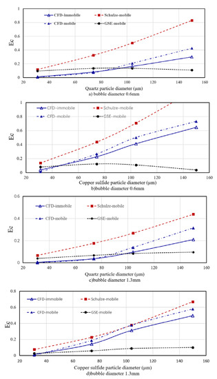
Figure 11.
Comparison of Schulze, GSE, and CFD simulation models for collision efficiency for bubble diameters of 0.6 mm (a,b) and 1.3 mm (c,d), and particle densities of 2650 kg/m3 (a,c) and 5600 kg/m3 (b,d).
It can be seen from Figure 11 that the results given by the three models are effectively the same as the collision efficiency law under the conditions of a mobile surface bubble. When the particle diameter is small, the calculation results of the three models are relatively consistent (because the inertial force can be ignored), and the collision efficiency given by the Schulze model is slightly higher. However, when the particle diameter is large, the calculation results of the three models differ greatly: the calculation results of the GSE model are smaller than when the particles are smaller, while the calculation results of the Schulze model are the same as for the CFD model, but the Schulze model collision efficiency is significantly higher.
When the particle diameter and density are large, due to the lack of calculation of the centrifugal (negative) inertial effect, and because the inertial effect is dominant, the calculation results of the Schulze model are higher than the CFD model results. Because the centrifugal (negative) inertial effect is overestimated, the centrifugal (negative) inertial effect in the GSE model increases with the increase in particle diameter, and the rate of increase of this negative inertial effect also increases at the same time. The difference between the GSE model and the other two models increases with the increase in bubble size. The calculation result of the GSE model increases first and then decreases under the condition that the bubble diameter is small (0.6 mm). When the bubble size is large (1.3 mm), this trend is not obvious. In addition, the Schulze model has a collision efficiency of greater than 1 for copper particles (particle density 5600 kg/m3) with a diameter of 150 μm. Therefore, if the Schulze model is used in the application, and if the predicted value is greater than 1, the efficiency should be set to 1.
5. Conclusions
Although the GSE model takes into account the centrifugal inertia effect (which is ignored in the Schulze model), comparisons with computational fluid dynamics simulation results showed that it overestimates this effect. In this regard, the conclusions of this paper are contrary to previous conclusions, which argue that the GSE model is more accurate. Computational fluid dynamics simulation results showed that the Schulze model is more accurate than the GSE model.
For immobile bubbles, the volume of fluid around the bubbles is reduced, but there is a connected fluid area where the bubbles are staggered farther apart, and the wake flow causes significant interference. The fluid velocity on both sides of the mobile bubble is significantly higher than the fluid velocity in this area under immobile surface conditions.
According to the computational fluid dynamics simulation results, it can be seen that when the particle diameter and particle density are large, the collision efficiency of the bubble under immobile surface conditions is greater than the collision efficiency under the conditions of mobile surface bubbles. Conversely, when the particle diameter and particle density are small, the collision efficiency of the bubbles under immobile surface conditions is smaller than the collision efficiency under the conditions of mobile surface bubbles.
Author Contributions
S.L.: Investigation, Writing—original draft, Writing—review & editing Methodology. K.J.: Supervision, Funding acquisition, Project administration. C.S.: Funding acquisition. All authors have read and agreed to the published version of the manuscript.
Funding
This research received no external funding.
Conflicts of Interest
The authors declare that they have no known competing financial interests or personal relationships that could have appeared to influence the work reported in this paper.
Abbreviations
| Roman | |
| a | Fitting parameter |
| b | Fitting parameter |
| Db | Bubble diameter |
| Dp | Particle diameter |
| Ec | Collision efficiency |
| Interceptional component of collision efficiency | |
| Interceptional component of collision efficiency as given by Sutherland | |
| Gravitational component of collision efficiency | |
| Ecin | Inertial component of collision efficiency |
| Etot | Total collision efficiency, as the sum of three components |
| Collision efficiency as given by the GSE model | |
| f | Parameter in the GSE model related to surface fluidity |
| Fi | Force on the ith particle |
| FD | Drag force on particle |
| FG | Gravitational force on particle |
| FP | Pressure force on particle |
| FA | Added mass force on particle |
| g | Acceleration due to gravity |
| G | Non-dimensionalized terminal velocity of the particle, Vp/Ub |
| K | Ratio of the particle inertial force to the drag force |
| K3 | Modified Stokes number |
| mp | Mass of particle |
| p | Pressure |
| r | Radial coordinate (i.e., distance from the center of the bubble) |
| Rb | Bubble radius |
| Rc | Distance of the critical flow line from vertical at a large distance |
| Rp | Particle radius |
| Re | Bubble Reynolds number |
| xi | Position of the ith particle (vector) |
| X | Non-dimensional radial co-ordinate, r/Rb |
| u | Fluid velocity (vector) |
| Ub | Velocity of bubble relative to surrounding liquid |
| vi | Velocity of the ith particle (vector) |
| Vp | Terminal velocity of particle |
| Greek | |
| β | Parameter in the GSE model |
| ρ | Liquid density |
| ρp | Particle density |
| μ | Liquid dynamic viscosity |
| ψ | Stokes (axisymmetric) stream-function |
| ψc | Value of stream-function for critical (grazing) streamline |
| Non-dimensionalized value of stream-function for critical streamline | |
| θ | Angular coordinate (angle from the vertical) |
| θc | Angle of the collision point of the critical grazing trajectory |
| θt | Parameter in the GSE model |
References
- Koh, P.T.L.; Schwarz, M.P. CFD modelling of bubble–particle attachments in flotation cells. Miner. Eng. 2006, 19, 619–626. [Google Scholar] [CrossRef]
- Mika, T.S.; Fuerstenau, D.W. A microscopic model of the flotation process. In Proceedings of the VIII International Mineral Processing Congress (IMPC), Leningrad, Russia, 10–15 June 1968; pp. 246–269. [Google Scholar]
- Li, S.; Schwarz, M.P.; Feng, Y.; Peter Witt, P.J.; Sun, C. A CFD Study of Particle–Bubble Collision Efficiency in Froth Flotation. Miner. Eng. 2019, 141, 105855. [Google Scholar] [CrossRef]
- Schulze, H.J. Hydrodynamics of bubble-mineral particle collisions. Min. Procesing Extr. Metall. Rev. 1989, 5, 43–76. [Google Scholar] [CrossRef]
- Dukhin, S.S. Role of inertial forces in flotation of small particles. Kolloid. Zh. 1982, 44, 431–441. [Google Scholar]
- Hassanzadeh, A.; Azizi, A.; Kouachi, S.; Karimi, M.; Celik, M.S. Estimation of flotation rate constant and particle-bubble interactions considering key hydrodynamic parameters and their interrelations. Miner. Eng. 2019, 141, 105836. [Google Scholar] [CrossRef]
- Verrelli, D.I.; Koh, P.T.L.; Nguyen, A.V. Particle–bubble interaction and attachment in flotation. Chem. Eng. Sci. 2011, 66, 5910–5921. [Google Scholar] [CrossRef]
- Weber, M.E.; Paddock, D. Interceptional and Gravitational Collision Efficiencies for Single Collector at Intermediate Reynolds Numbers. J. Colloid Interface Sci. 1983, 94, 328–335. [Google Scholar] [CrossRef]
- Nguyen, A.V.; Evans, G.M. Exact and global rational approximate expressions for resistance coefficients for a colloidal solid sphere moving in a quiescent liquid parallel to a slip gas–liquid interface. J. Colloid Interface Sci. 2004, 273, 262–270. [Google Scholar] [CrossRef] [PubMed]
- Flint, L.R.; Howarth, W.J. Collision efficiency of small particles with spherical air bubbles. Chem. Eng. Sci. 1971, 26, 1155–1168. [Google Scholar] [CrossRef]
- Dai, Z.; Dukhin, S.; Fornasiero, D.; Ralston, J. The inertial hydrodynamic interaction of particles and rising bubbles with mobile surfaces. J. Colloid Interface Sci. 1998, 197, 275–292. [Google Scholar] [CrossRef]
- Legendre, D.; Magnaudet, J. A note on the lift force on a spherical bubble or drop in a low-Reynolds-number shear flow. Phys. Fluids 1997, 9, 3572. [Google Scholar] [CrossRef]
© 2020 by the authors. Licensee MDPI, Basel, Switzerland. This article is an open access article distributed under the terms and conditions of the Creative Commons Attribution (CC BY) license (http://creativecommons.org/licenses/by/4.0/).