Seabed Mapping Using Shipboard Multibeam Acoustic Data for Assessing the Spatial Distribution of Ferromanganese Crusts on Seamounts in the Western Pacific


Abstract
1. Introduction
2. Materials and Methods
2.1. MBES Data Acquisition and Processing
2.2. Seafloor Observation Using Camera Tow
3. Results
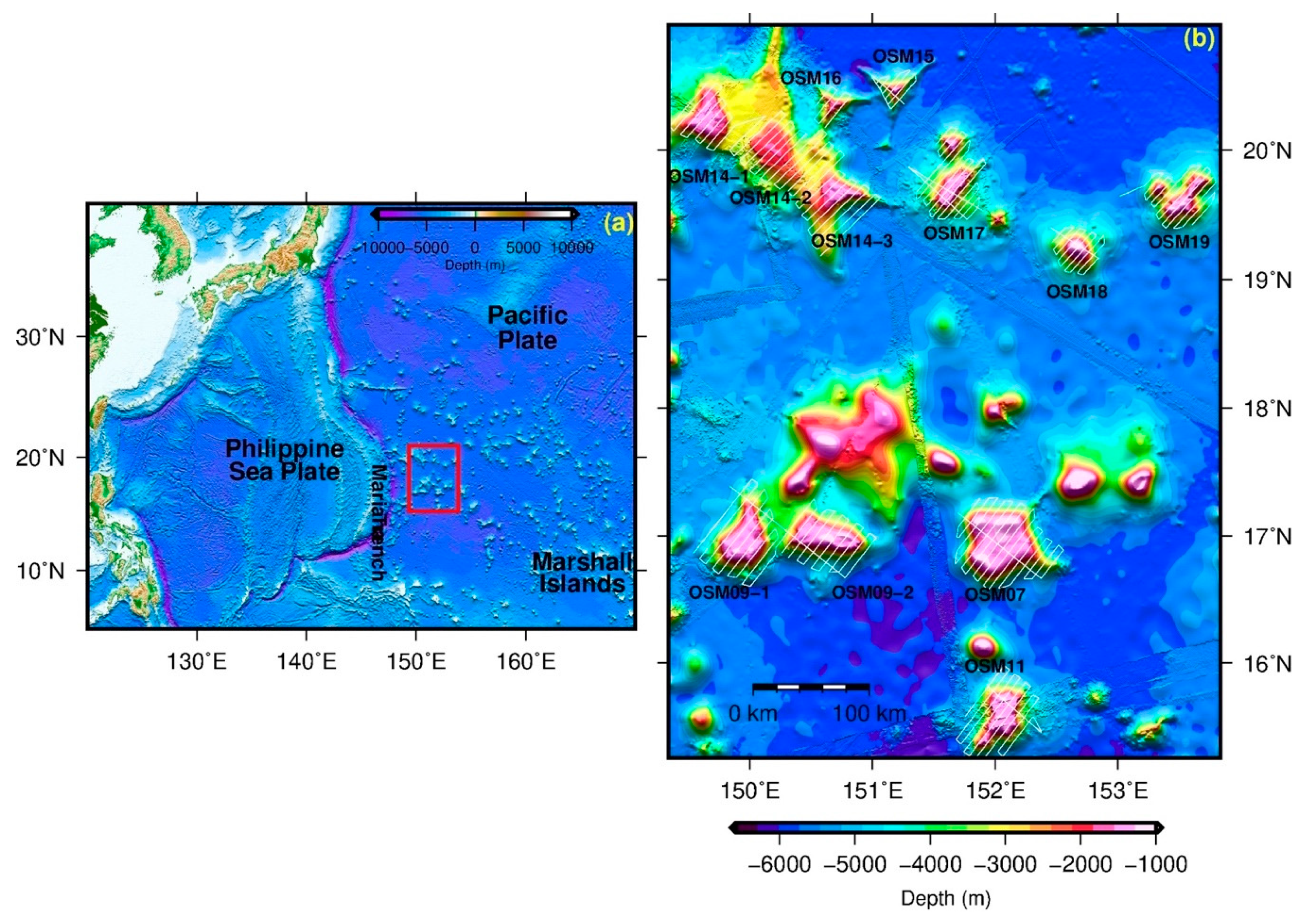
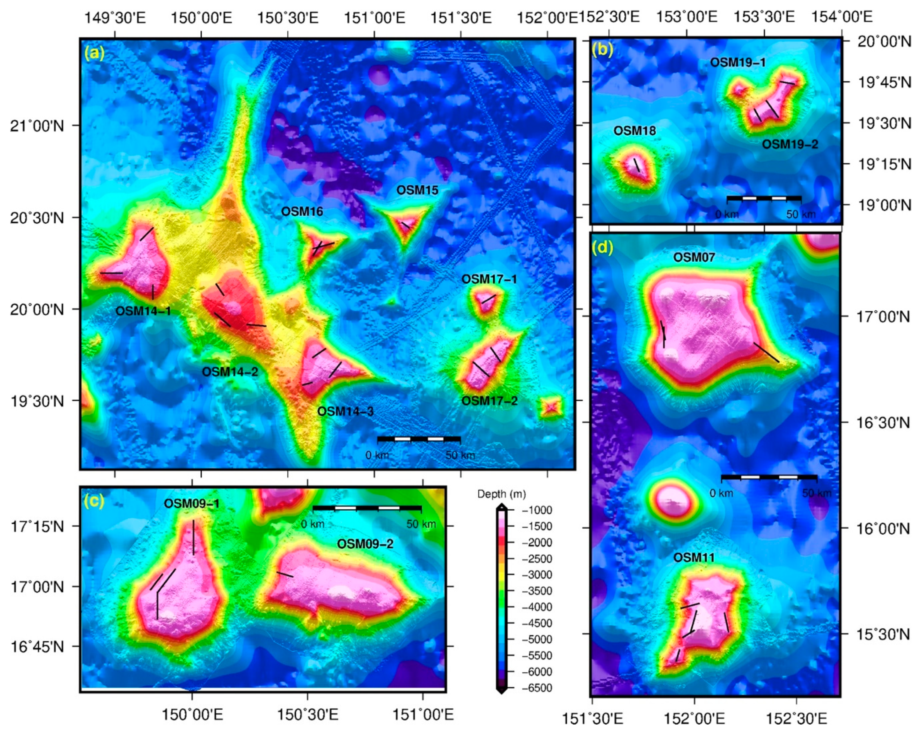
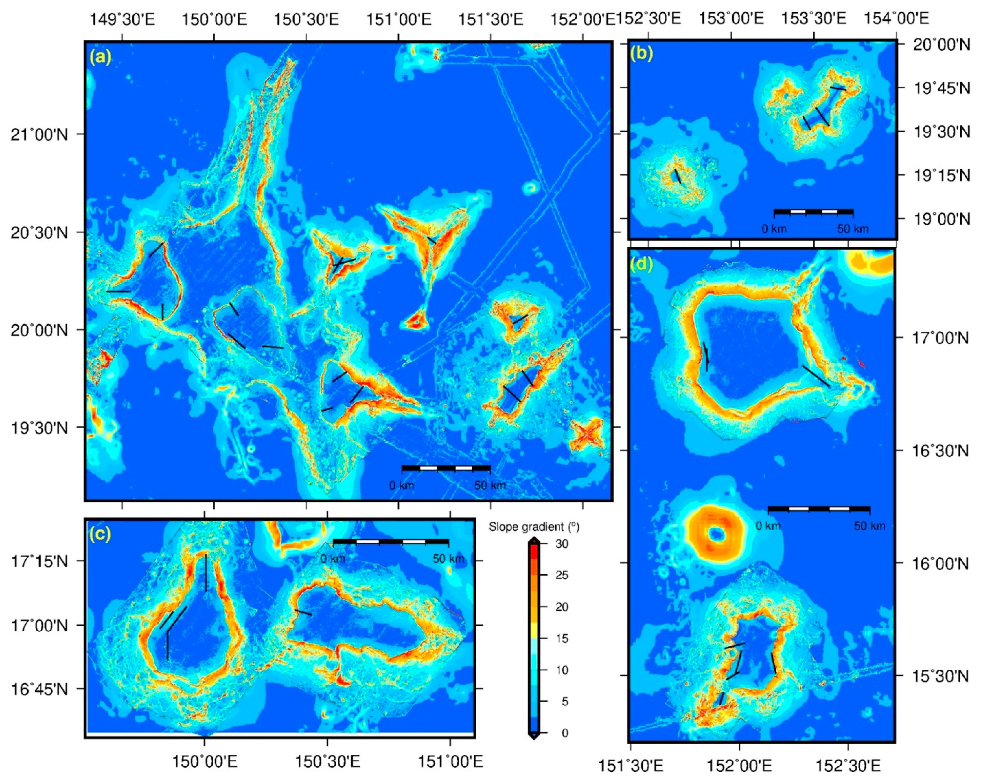
3.1. Seafloor Morphology
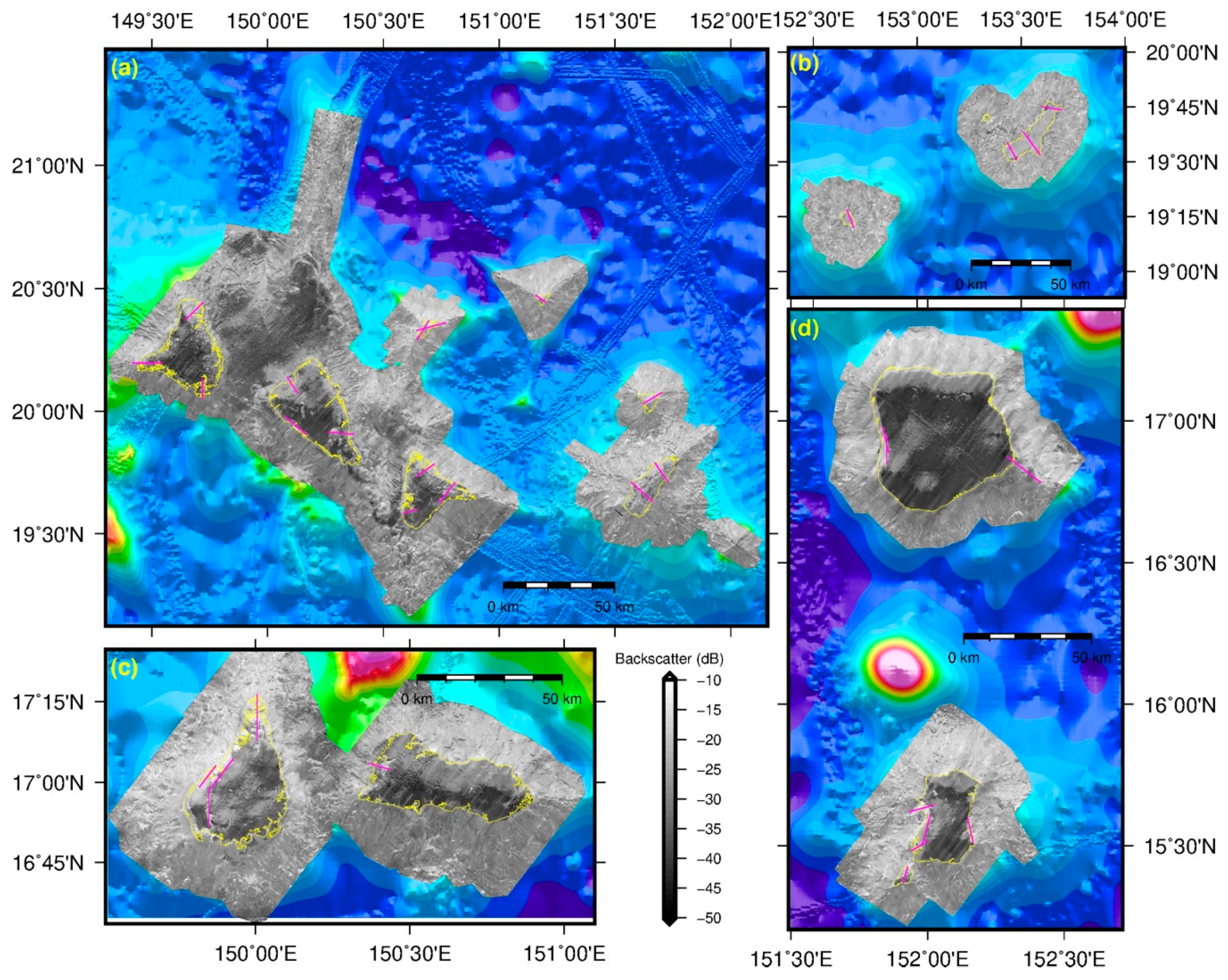
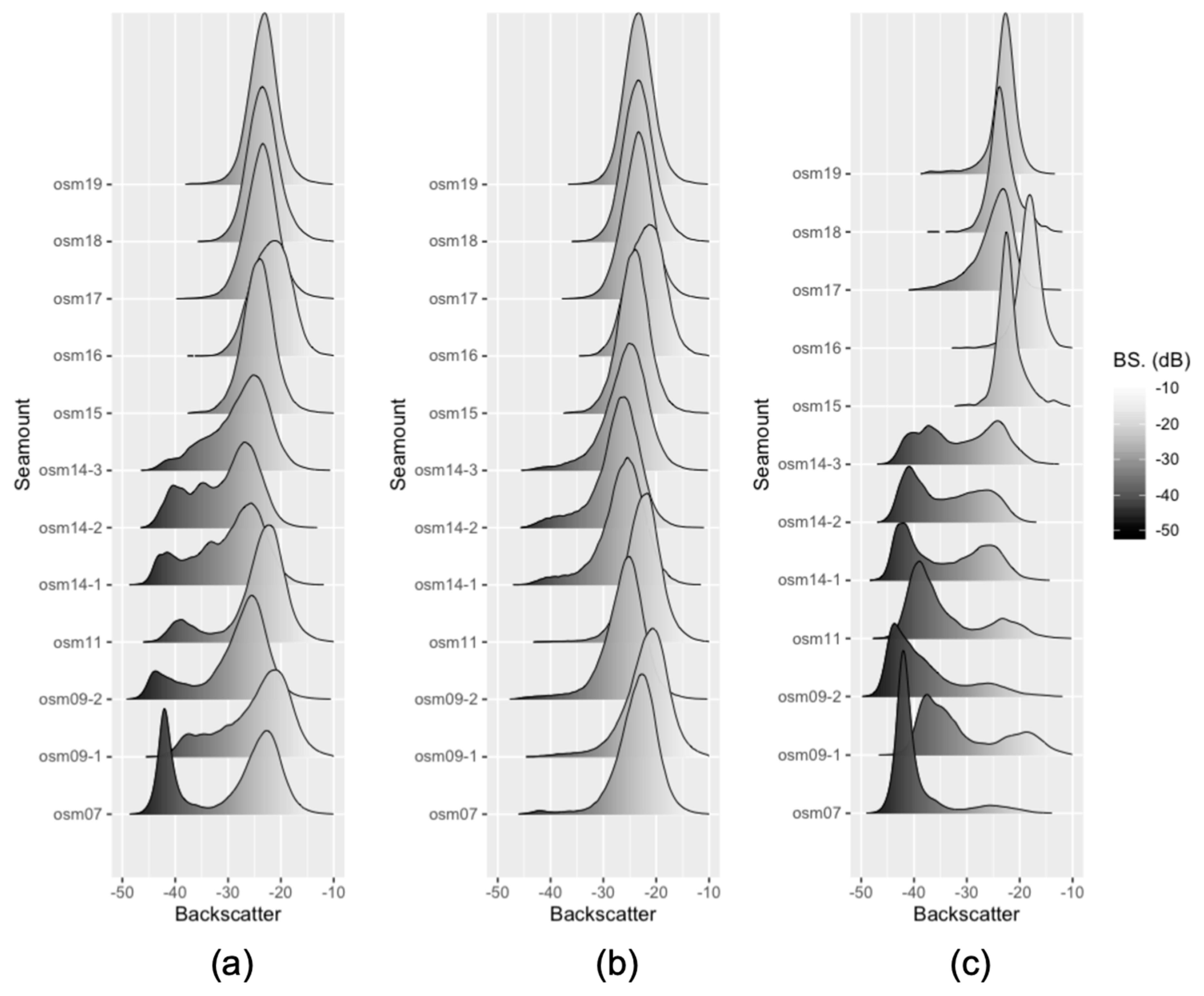
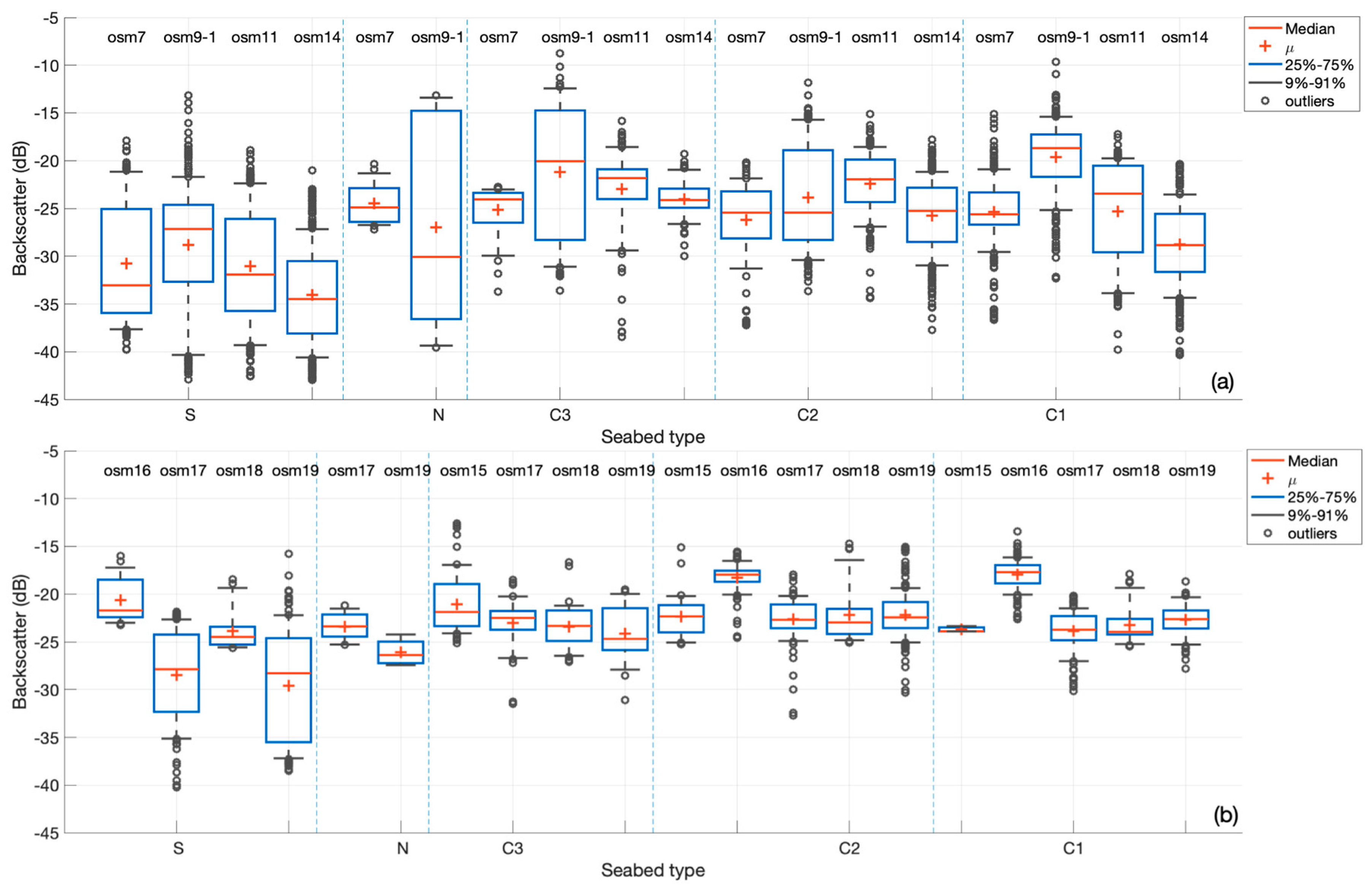
3.2. Seabed Backscatter Intensity
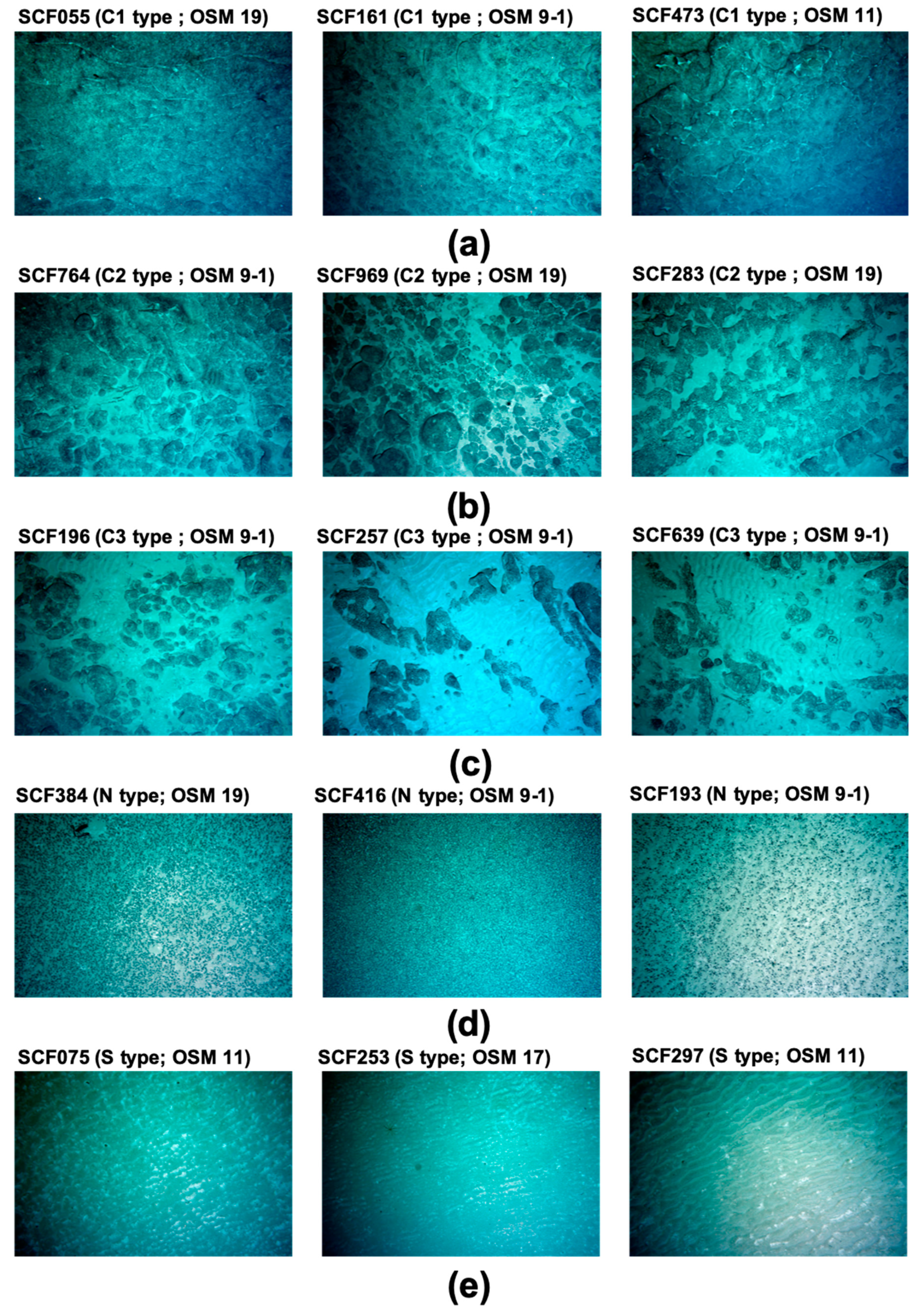
3.3. Seafloor Video Characterizations
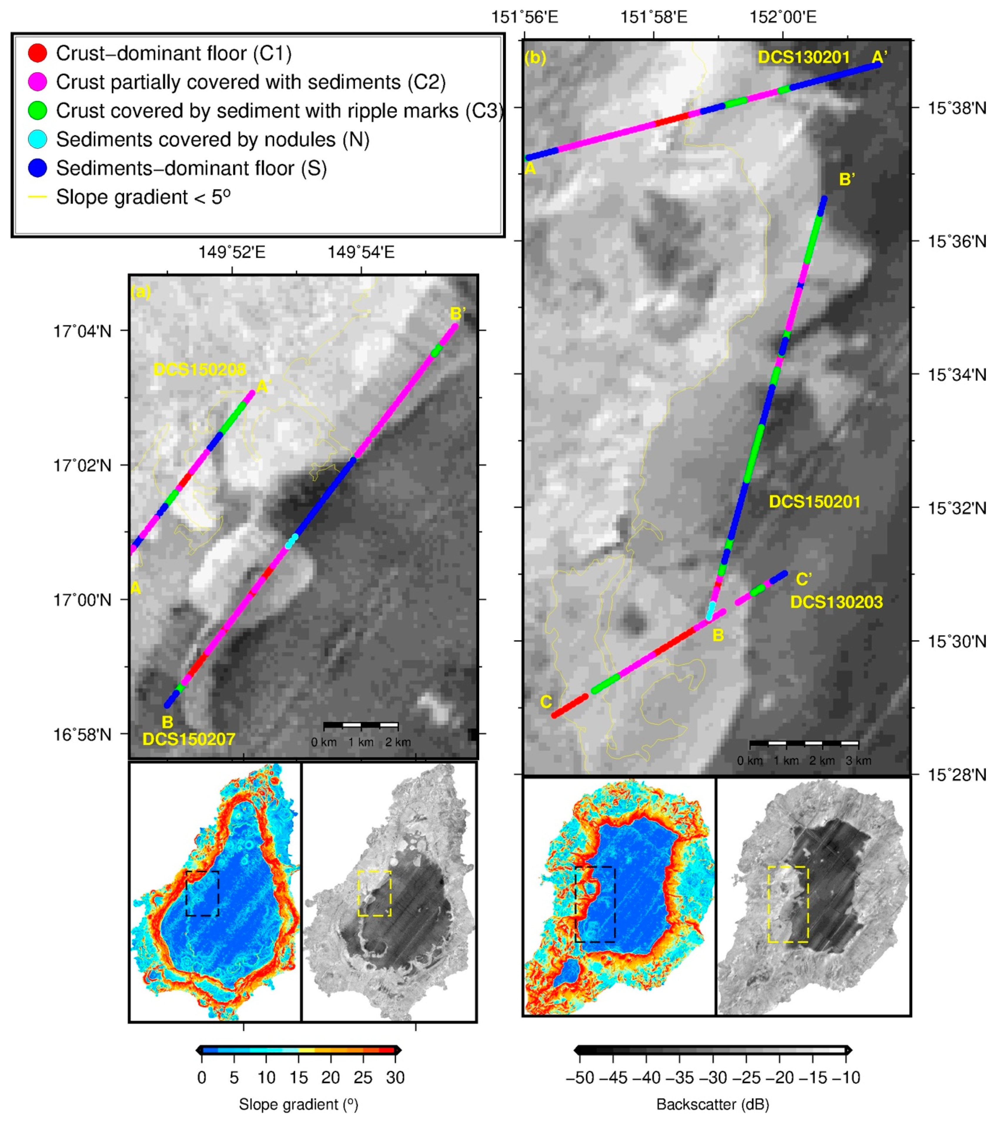
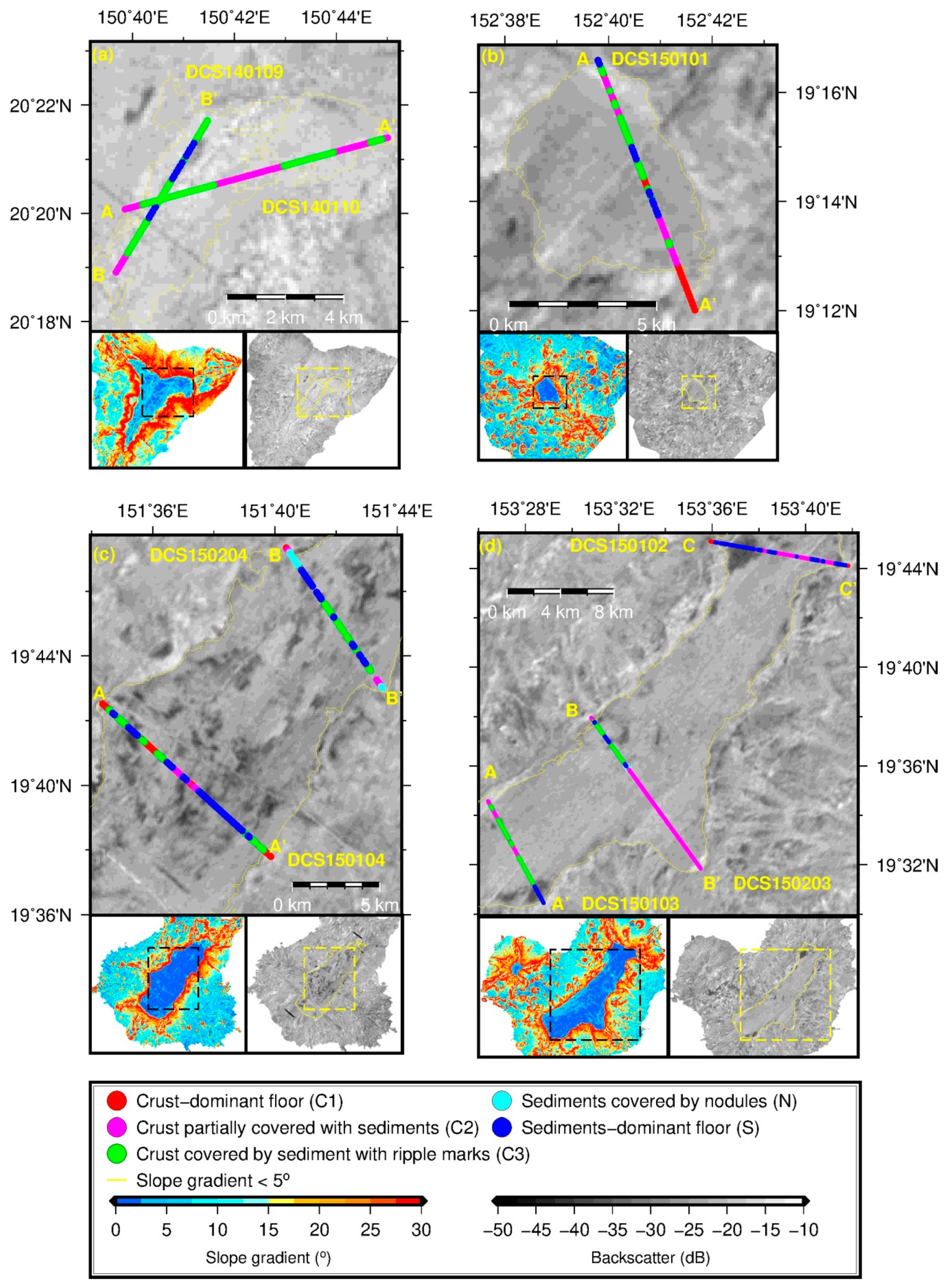
3.4. Comparison between MBES Backscatter and Video Footage
4. Discussion
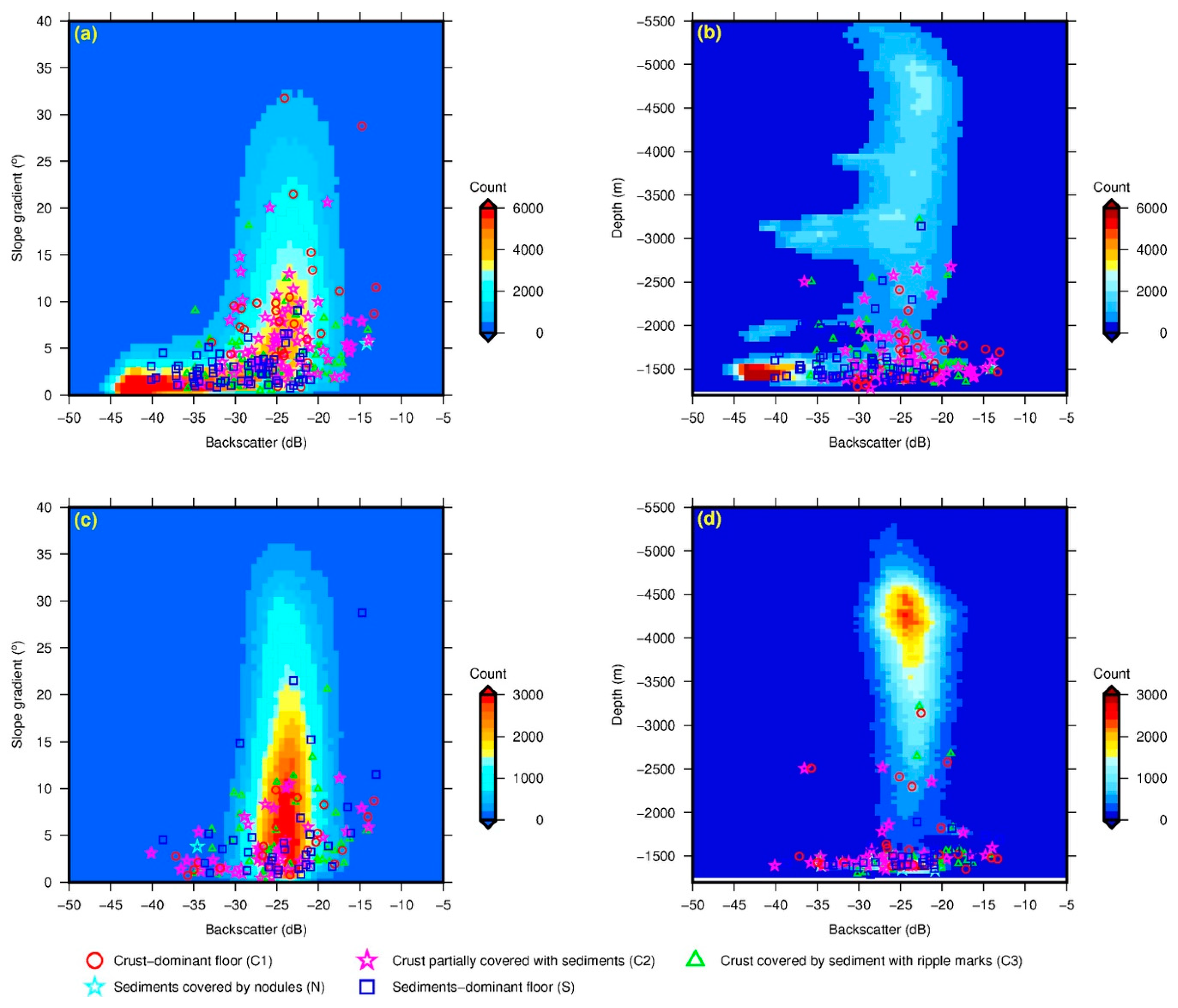
4.1. Factors Affecting MBES Backscatter
4.2. Relationship between MBES Backscatter and Occurrence of Fe–Mn Crusts
5. Conclusions
Author Contributions
Funding
Acknowledgments
Conflicts of Interest
References
- Usui, A.; Okamoto, N. Geophysical and geological exploration of Cobalt-rich ferromanganese crusts: An attempt of small-scale mapping on a Micronesian seamount. Mar. Georesour. Geotechnol. 2010, 28, 192–206. [Google Scholar] [CrossRef]
- Hein, J.R.; Mizell, K.; Koschinsky, A.; Conrad, T.A. Deep-ocean mineral deposits as a source of critical metals for high-and green-technology applications: Comparison with land-based resources. Ore Geol. Rev. 2013, 51, 1–14. [Google Scholar] [CrossRef]
- Kim, J.; Ko, Y.; Hyeong, K.; Moon, J.W. Geophysical and geological exploration of cobalt-rich ferromanganese Crusts on a seamount in the Western Pacific. Econ. Environ. Geol. 2013, 46, 569–580. [Google Scholar] [CrossRef][Green Version]
- Scheirer, D.S.; Fornari, D.J.; Humphris, S.E.; Lerner, S. High-resolution seafloor mapping using the DSL-120 sonar system: Quantitative assessment of sidescan and phase-bathymetry data from the Lucky Strike segment of the Mid-Atlantic Ridge. Mar. Geophys. Res. 2000, 21, 121–142. [Google Scholar] [CrossRef]
- Sen, A.; Ondreas, H.; Gaillot, A.; Marcon, Y.; Augustin, J.M.; Olu, K. The use of multibeam backscatter and bathymetry as a means of identifying faunal assemblages in a deep-sea cold seep. Deep Sea Res. Part I 2016, 110, 33–49. [Google Scholar] [CrossRef]
- Siwabessy, P.J.W.; Tran, M.; Picard, K.; Brooke, B.P.; Huang, Z.; Smit, N.; Williams, D.K.; Nicholas, W.A.; Nichol, S.L.; Atkinson, I. Modelling the distribution of hard seabed using calibrated multibeam acoustic backscatter data in a tropical, macrotidal embayment: Darwin Harbour, Australia. Mar. Geophys. Res. 2018, 39, 249–269. [Google Scholar] [CrossRef]
- Yoshikawa, S.; Okino, K.; Asada, M. Geomorphological variations at hydrothermal sites in the southern Mariana Trough: Relationship between hydrothermal activity and topographic characteristics. Mar. Geol. 2012, 303, 172–182. [Google Scholar] [CrossRef]
- Thornton, B.; Asada, A.; Bodenmann, A.; Sangekar, M.; Ura, T. Instruments and methods for acoustic and visual survey of manganese crusts. IEEE J. Ocean Eng. 2013, 38, 186–203. [Google Scholar] [CrossRef]
- Wilson, M.F.J.; O’Connell, B.; Brown, C.; Guinan, J.C.; Grehan, A.J. Multiscale terrain analysis of multibeam bathymetry data for habitat mapping on the continental slope. Mar. Geod. 2007, 30, 3–35. [Google Scholar] [CrossRef]
- Brown, C.J.; Smith, S.J.; Lawton, P.; Anderson, J.T. Benthic habitat mapping: A review of progress towards improved understanding of the spatial ecology of the seafloor using acoustic techniques. Estuar. Coast. Shelf Sci. 2011, 92, 502–520. [Google Scholar] [CrossRef]
- Parnum, I.M.; Gavrilov, A.N. High-frequency multibeam echo-sounder measurements of seafloor backscatter in shallow water: Part 1—Data acquisition and processing. J. Underw. Technol. 2011, 30, 3–12. [Google Scholar] [CrossRef]
- Micallef, A.; Le Bas, T.P.; Huvenne, V.A.I.; Blondel, P.; Hühnerbach, V.; Deidun, A. A multi-method approach for benthic habitat mapping of shallow coastal areas with high-resolution multibeam data. Cont. Shelf. Res. 2012, 39–40, 14–26. [Google Scholar] [CrossRef]
- De Moustier, C.P. Beyond bathymetry: Mapping acoustic backscattering from the deep seafloor with Sea Beam. J. Acoust. Soc. Am. 1986, 79, 316–331. [Google Scholar] [CrossRef]
- Weydert, M. Measurement of Acoustic Backscattering of the Deep Seafloor Using a Deeply Towed Vehicle. A Technique to Investigate the Physical and Geological Properties of the Deep Seafloor and to Assess Manganese Nodule Resources. Ph.D. Thesis, University of California, San Diego, CA, USA, 1985. [Google Scholar]
- Lee, S.H.; Kim, K.H. Side-scan sonar characteristics and manganese nodule abundance in the Clarion-Clipperton Fracture Zones NE equatorial Pacific. Mar. Georesour. Geotechnol. 2004, 22, 103–114. [Google Scholar] [CrossRef]
- Ko, Y.; Lee, S.; Kim, J.; Kim, K.H.; Jung, M.S. Relationship between Mn nodule abundance and other geological factors in the northeastern Pacific: Application of GIS and probability method. Ocean Sci. J. 2006, 41, 149–161. [Google Scholar] [CrossRef]
- Alevizos, E.; Schoening, T.; Koeser, K.; Snellen, M.; Greinert, J. Quantification of the fine-scale distribution of Mn-nodules: Insights from AUV multi-beam and optical imagery data fusion. Biogeosci. Discuss. 2018. in review. [Google Scholar] [CrossRef]
- Ferrini, V.L.; Flood, R.D. The effects of fine-scale surface roughness and grain size on 300 kHz multibeam backscatter intensity in sandy marine sedimentary environments. Mar. Geol. 2006, 228, 153–172. [Google Scholar] [CrossRef]
- Sutherland, T.F.; Galloway, J.; Loschiavo, R.; Levings, C.D.; Hare, R. Calibration techniques and sampling resolution requirements for groundtruthing multibeam acoustic backscatter (EM3000) and QTC VIEW classification technology. Estuar. Coast. Shelf Sci. 2007, 75, 447–458. [Google Scholar] [CrossRef]
- Jackson, D.R.; Winebrenner, D.P.; Ishimaru, A. Application of the composite roughness model to high-frequency bottom backscatter. J. Acoust. Soc. Am. 1986, 79, 1410–1422. [Google Scholar] [CrossRef]
- Jackson, D.R.; Briggs, K.B.; Williams, K.L.; Richardson, M.D. Tests of models for high-frequency seafloor backscatter. IEEE J. Ocean Eng. 1996, 21, 458–470. [Google Scholar] [CrossRef]
- de Moustier, C.P.; Alexandrou, D. Angular dependence of 12-kHz seafloor acoustic backscatter. J. Acoust. Soc. Am. 1991, 90, 522–531. [Google Scholar] [CrossRef]
- APL. APL-UW High-Frequency Ocean Environment Acoustic Models Handbook (APL-UW TR9407); Applied Physics Laboratory, University of Washington: Seattle, WA, USA, 1994; pp. 1–49. [Google Scholar]
- Clarke, J.E. Towards remote seafloor classification using the angular response of acoustic backscattering: A case study from multiple overlapping GLORIA data. IEEE J. Ocean Eng. 1994, 19, 112–127. [Google Scholar] [CrossRef]
- Talukdar, K.K.; Tyce, R.C.; Clay, C.S. Interpretation of Sea Beam backscatter data collected at the Laurentian fan off Nova Scotia using acoustic backscatter theory. J. Acoust. Soc. Am. 1995, 97, 1545–1558. [Google Scholar] [CrossRef]
- Novarini, J.C.; Caruthers, J.W. A simplified approach to backscattering from a rough seafloor with sediment inhomogeneities. IEEE J. Ocean Eng. 1998, 23, 157–166. [Google Scholar] [CrossRef]
- Williams, K.L.; Jackson, D.R.; Thorsos, E.I.; Tang, D.; Briggs, K.B. Acoustic backscattering experiments in a well characterized sand sediment: Data/model comparisons using sediment fluid and Biot models. IEEE J. Ocean Eng. 2002, 27, 376–387. [Google Scholar] [CrossRef]
- Fonseca, L.; Mayer, L. Remote estimation of surficial seafloor properties through the application angular range analysis to multibeam sonar data. Mar. Geophys. Res. 2007, 28, 119–126. [Google Scholar] [CrossRef]
- Parnum, I.M. Benthic Habitat Mapping Using Multibeam Sonar Systems. Ph.D. Thesis, Curtin University of Technology, Perth, Australia, 2007. [Google Scholar]
- Gavrilov, A.N.; Parnum, I.M. Fluctuations of seafloor backscatter data from multibeam sonar systems. IEEE J. Ocean Eng. 2010, 35, 209–219. [Google Scholar] [CrossRef]
- Hamilton, L.J.; Parnum, I.M. Acoustic seabed segmentation from direct statistical clustering of entire multibeam sonar backscatter curves. Cont. Shelf Res. 2011, 31, 138–148. [Google Scholar] [CrossRef]
- Hasan, R.C.; Ierodiaconou, D.; Laurenson, L. Combining angular response classification and backscatter imagery segmentation for benthic biological habitat mapping. Estuar. Coast. Shelf Sci. 2012, 97, 1–9. [Google Scholar] [CrossRef]
- Lurton, X.; Lamarche, G.; Brown, C.; Lucieer, V.L.; RIce, G.; Schimel, A.; Weber, T. Backscatter Measurements by Seafloor-Mapping Sonars. Guidelines and Recommendations. Collect. Rep. Memb. GeoHab Backscatter Work. Gr. 2015, 5, 200. [Google Scholar]
- Stewart, W.K.; Chu, D.; Malik, S.; Lerner, S.; Singh, H. Quantitative seafloor characterization using a bathymetric sidescansonar. IEEE J. Ocean Eng. 1994, 19, 599–610. [Google Scholar] [CrossRef]
- Richardson, M.D.; Briggs, K.B.; Williams, K.L.; Lyons, A.P.; Jackson, D.R. Effects of changing roughness on acoustic scattering: (2) anthropogenic changes. Proc. Inst. Acoust. 2001, 23, 343–390. [Google Scholar]
- Briggs, K.B.; Tang, D.; Williams, K.L. Characterization of interface roughness of rippled sand off Fort Walton Beach, Florida. IEEE J. Ocean Eng. 2002, 27, 505–514. [Google Scholar] [CrossRef]
- Joo, J.; Kim, J.; Ko, Y.; Kim, S.S.; Son, J.; Pak, S.J.; Ham, D.J.; Son, S.K. Characterizing geomorphological properties of western pacific seamounts for cobalt-rich ferromanganese crust resource assessment. Econ. Environ. Geol. 2016, 49, 121–134. [Google Scholar] [CrossRef][Green Version]
- Ryan, W.B.F.; Carbotte, S.M.; Coplan, J.O.; O’Hara, S.; Melkonian, A.; Arko, R.; Weissel, R.A.; Ferrini, V.; Goodwillie, A.; Nitsche, F.; et al. Global Multi-Resolution Topography synthesis. Geochem. Geophys. Geosyst. 2009, 10, Q03014. [Google Scholar] [CrossRef]
- Caress, D.W.; Chayes, D.N. MB-System: Mapping the Seafloor. 2006. Available online: http://www.mbari.org/data/mbsystem (accessed on 6 January 2014).
- Wessel, P.; Smith, W.H.F.; Scharroo, R.; Luis, J.F.; Wobbe, F. Generic mapping tools: Improved version released. Eos Trans. AGU 2013, 94, 409–410. [Google Scholar] [CrossRef]
- Hellequin, L.; Lurton, X.; Augustin, J.M. Postprocessing and signal corrections for multibeam echosounder images. In Proceedings of the Oceans ’97, MTS/IEEE Conference, Halifax, NS, Canada, 6–9 October 1997; pp. 23–26. [Google Scholar]
- Hellequin, L.; Boucher, J.M.; Lurton, X. Processing of high-frequency multibeam echo sounder data for seafloor characterization. IEEE J. Ocean Eng. 2003, 28, 78–89. [Google Scholar] [CrossRef]
- Le Gonidec, Y.; Lamarche, G.; Wright, I.C. Inhomogeneous Substrate Analysis Using EM300 Backscatter Imagery. Mar. Geophys. Res. 2003, 24, 311–327. [Google Scholar] [CrossRef]
- Lamarche, G.; Lurton, X.; Verdier, A.L.; Augustin, J.M. Quantitative characterization of seafloor substrate and bedforms using advanced processing of multibeam backscatter—Application to the Cook Strait, New Zealand. Cont. Shelf Res. 2011, 31, S93–S109. [Google Scholar] [CrossRef]
- Fonseca, L.; Calder, B. Geocoder: An efficient backscatter map constructor. In Proceedings of the U.S. Hydrographic Conference 2005, San Diego, CA, USA, 29–31 March 2005; pp. 1–9. [Google Scholar]
- Blondel, P. Handbook of Sidescan Sonar; Springer: New York, NY, USA, 2009; pp. 15–18. [Google Scholar]
- Lurton, X. An Introduction to Underwater Acoustics: Principles and Applications, 2nd ed.; Springer Praxis Publishing: London, UK, 2010; pp. 85–102. [Google Scholar]
- Innangi, S.; Passaro, S.; Tonielli, R.; Mailano, G.; Ventura, G.; Tamburrino, S. Seafloor mapping using high-resolution multibeam backscatter: The Palinuro Seamount (Eastern Tyrrhenian Sea). J. Maps 2016, 12, 736–746. [Google Scholar] [CrossRef]
- Urick, R.J. The backscattering of Sound from a Harbor Bottom. J. Acoust. Soc. Am. 1954, 26, 231–235. [Google Scholar] [CrossRef]
- Williams, K.L.; Jackson, D.A.; Tang, D.; Briggs, K.B.; Thorsos, E.I. Acoustic backscattering from a sand and a sand/mud environment: Experiments and data/model comparisons. IEEE J. Ocean Eng. 2009, 34, 388–398. [Google Scholar] [CrossRef]
- Yoo, C.H.; Joo, J.; Lee, S.H.; Ko, Y.; Chi, S.B.; Kim, H.J.; Seo, I.; Hyeong, K. Resource Assessment of Polymetallic Nodules Using Acoustic Backscatter Intensity Data from the Korean Exploration Area, Northeastern Equatorial Pacific. Ocean Sci. J. 2018, 53, 381–394. [Google Scholar] [CrossRef]
- Clarke, J.E. Multispetral acoustic backscatter from multibeam, improved classification potential. In Proceedings of the U.S. Hydrographic Conference 2015, National Harbor, MD, USA, 16–19 March 2015; pp. 1–18. [Google Scholar]
- Brown, C.J.; Beaudoin, J.; Brissette, M.; Gazzola, V. Setting the Stage for Multispectral Acoustic Backscatter Research. In Proceedings of the United States Hydrographic Conference, Galveston, TX, USA, 20–23 March 2017. [Google Scholar]
- Gaida, T.C.; Ali, T.A.; Snellen, M.; Amiri-Simkooei, A.; Dijk, T.A.; Simons, D.G. A multispectral bayesian classification method for increased acoustic discrimination of seabed sediments using multi-frequency multibeam backscatter data. Geosciences 2018, 8, 455. [Google Scholar] [CrossRef]


| Seabed Type | Depth (m) | Slope Gradients (°) | Backscatter Intensity (dB) |
|---|---|---|---|
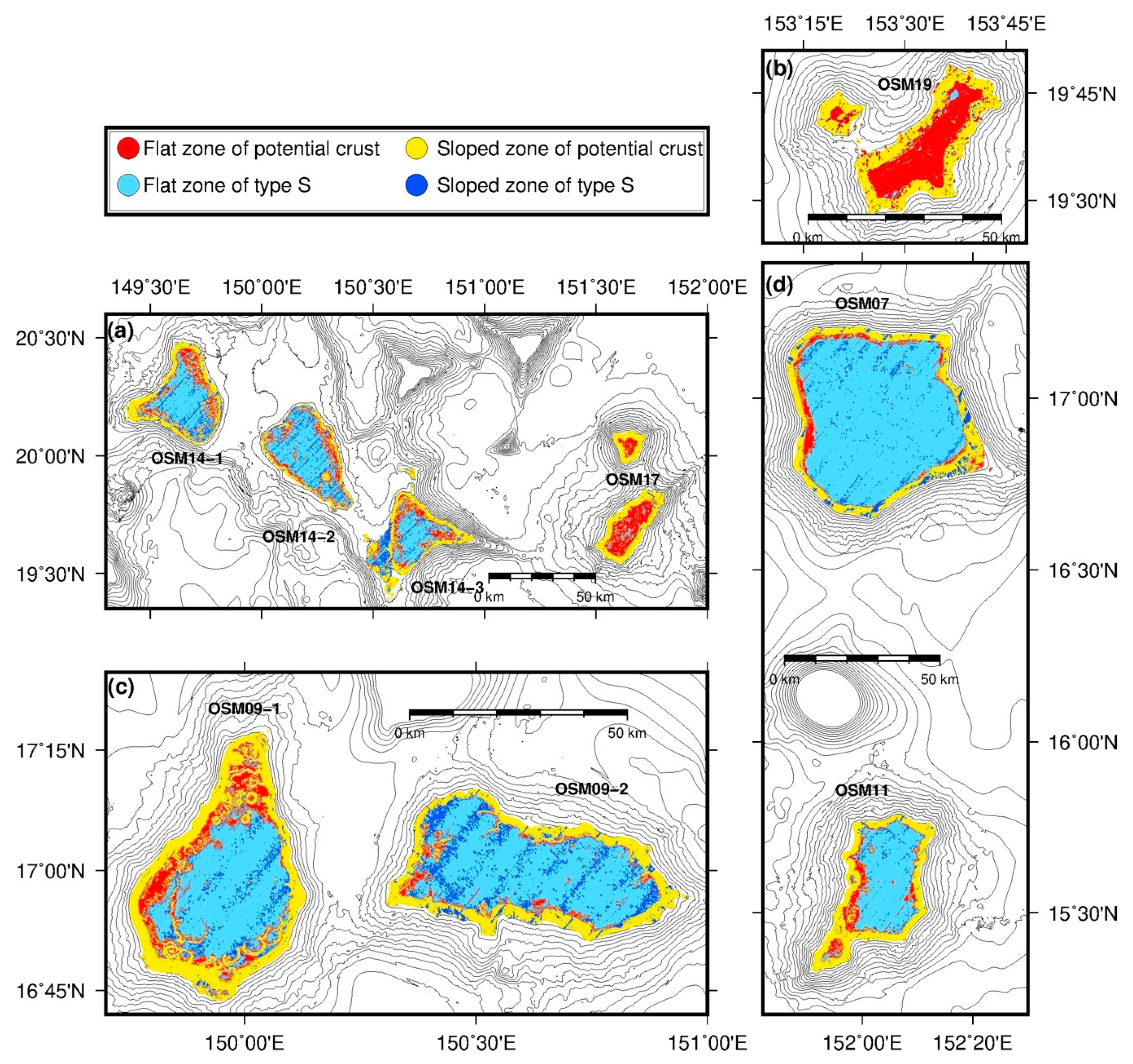
| Flat zone of type S | >2500 | <5 | <−30 |
| Flat zone of potential crust | >−30 | ||
| Sloped zone of type S | >5 | <−30 | |
| Sloped zone of potential crust | >−30 |
| Target | Potential Crust | Type S |
|---|---|---|
| Transect‘s points correctly classified | 2058 | 668 |
| Transect‘s points incorrectly classified | 617 | 471 |
| Total | 2675 | 1139 |
| Accuracy Rate | 78% | 59% |
© 2020 by the authors. Licensee MDPI, Basel, Switzerland. This article is an open access article distributed under the terms and conditions of the Creative Commons Attribution (CC BY) license (http://creativecommons.org/licenses/by/4.0/).
Share and Cite
Joo, J.; Kim, S.-S.; Choi, J.W.; Pak, S.-J.; Ko, Y.; Son, S.-K.; Moon, J.-w.; Kim, J. Seabed Mapping Using Shipboard Multibeam Acoustic Data for Assessing the Spatial Distribution of Ferromanganese Crusts on Seamounts in the Western Pacific. Minerals 2020, 10, 155. https://doi.org/10.3390/min10020155
Joo J, Kim S-S, Choi JW, Pak S-J, Ko Y, Son S-K, Moon J-w, Kim J. Seabed Mapping Using Shipboard Multibeam Acoustic Data for Assessing the Spatial Distribution of Ferromanganese Crusts on Seamounts in the Western Pacific. Minerals. 2020; 10(2):155. https://doi.org/10.3390/min10020155
Chicago/Turabian StyleJoo, Jongmin, Seung-Sep Kim, Jee Woong Choi, Sang-Joon Pak, Youngtak Ko, Seung-Kyu Son, Jai-woon Moon, and Jonguk Kim. 2020. "Seabed Mapping Using Shipboard Multibeam Acoustic Data for Assessing the Spatial Distribution of Ferromanganese Crusts on Seamounts in the Western Pacific" Minerals 10, no. 2: 155. https://doi.org/10.3390/min10020155
APA StyleJoo, J., Kim, S.-S., Choi, J. W., Pak, S.-J., Ko, Y., Son, S.-K., Moon, J.-w., & Kim, J. (2020). Seabed Mapping Using Shipboard Multibeam Acoustic Data for Assessing the Spatial Distribution of Ferromanganese Crusts on Seamounts in the Western Pacific. Minerals, 10(2), 155. https://doi.org/10.3390/min10020155