Dynamic Monitoring of Grinding Circuits by Use of Global Recurrence Plots and Convolutional Neural Networks

Abstract

Reliable control of grinding circuits is critical to more efficient operation of concentrator plants. In many cases, operators still play a key role in the supervisory control of grinding circuits but are not always able to act timely to deal with disturbances, such as changes in the mill feed. Reliable process monitoring can play a major role in assisting operators to take more timely and reliable action. These monitoring systems need to be able to deal with what could be complex nonlinear dynamic behavior of comminution circuits. To this end, a dynamic process monitoring approach is proposed based on the use of convolutional neural networks. To take advantage of the availability of pretrained neural networks, the grinding circuit variables are treated as time series which can be converted into images. Features extracted from these networks are subsequently analyzed in a multivariate process monitoring framework with an underlying principal component model. Two variants of the approach based on convolutional neural networks are compared with dynamic principal component analysis on a simulated and real-world case studies. In the first variant, the pretrained neural network is used as a feature extractor without any further training. In the second variant, features are extracted following further training of the network in a synthetic binary classification problem designed to enhance the extracted features. The second approach yielded nominally better results than what could be obtained with dynamic principal component analysis and the approach using features extracted by transfer learning.

1. Introduction

The energy efficient operation of grinding circuits remains paramount in the processing of minerals, as these circuits account for a major proportion of the energy consumed in concentrator operations. Optimal control of grinding circuits is key towards achieving these goals. Generally, the objective is to maintain a specific level of product quality (particle size) and to maximize throughput [1].

Although single loop proportional-integral-derivative (PID) controllers are still the norm for industrial milling circuit control, this approach is not always effective, as strong interactions between the loops is not accounted for [1]. As a consequence, advanced control systems have been developed, e.g., model predictive controllers [2,3,4], fuzzy logic [5], expert system controllers [6,7] and other nonlinear control systems, such as recently proposed by Inapakurthi et al. [8].

Despite these advances, the behavior of grinding circuits can be highly nonlinear and fully automated control may not be feasible in practice. This is particularly the case with autogenous grinding (AG) and semi-autogenous grinding circuits (SAG), where the behavior of the mill is strongly affected by the properties of the ore being ground.

Under these circumstances, human operators play a key role in the control of milling circuits and a sensible support strategy would be to support operator decisions, while pursuing the longer-term goal of developing fully automatic control systems. Operator support can include visualization of the mill behavior [9], rule-based or expert systems support [10,11] and multivariate statistical process control [12,13,14,15].

Process monitoring methods in particular are reinforced by the development of novel sensors to better interpret the behavior of the mill. This includes acoustic sensors [16,17], accelerometric measurement of the milling equipment [18] and the development of image processing to characterize particulate mill feed and product [19]. These sensors often have the same predictive power with regard to the performance of the grinding circuit as sets of operational variables, although interpretation of physical phenomena from these signals may be more challenging.

The use of dynamic monitoring methods exploiting key signals in mill operation have proliferated over the last few decades. One of the earliest approaches based on the use of principal component analysis was introduced by Ku et al. [20], by augmenting each process variable with a number of lagged samples before building the PCA model. While this approach can explicitly deal with dependencies in the samples in time series data, it is adversely affected by a number of issues. These include determination of a proper lag structure for the variables, where dependencies are not well captured by linear methods, such as the autocovariance of the time series. In addition, there is the challenge of dealing with a considerable increase in the dimensionality of the systems (number of variables), if the lag parameter is large. In particular, this could pose a problem in highly nonlinear systems, such as grinding circuits. Different ways of extending dynamic PCA have been investigated to address some of these problems [21]. This includes extension to nonlinear methods, such as dynamic kernel PCA [22], dynamic independent component analysis [23,24], dissimilarity methods [25,26] and support vector data description [27]. Another class of approaches is focused on distributed or decentralized models, to deal with nonlinear dynamic process behavior that arises owing to the existence of operating modes in the process [28].

Despite these advances, dynamic monitoring of nonlinear process systems remains an open research issue, and, in this paper, a dynamic monitoring methodology based on the use of convolutional neural networks is proposed. In this approach, measured signals are first converted into images, before features are extracted that can be interpreted in a classical multivariate process monitoring framework. This addresses a number of the major challenges facing dynamic process monitoring, as briefly outlined above, as it globally captures potentially highly nonlinear process dynamics within a sliding window, without suffering from the drawbacks of having to deal with high-dimensional systems in the usual way. To contextualize the performance of these approaches, they are compared with a dynamic principal component model.

In Section 2, the basic operation of convolutional neural networks is outlined, followed by Section 3, where the analytical methodology is explained. In Section 4, two illustrative case studies are considered, and the results are discussed in Section 5. The conclusions of the paper are summarized in Section 6.

2. Convolutional Neural Networks

Convolutional neural networks (CNNs) are deep neural networks that have been designed to learn features from images that can be used in a variety of pattern recognition tasks. Their architectures emulate the animal visual cortex and its powerful visual processing capabilities.

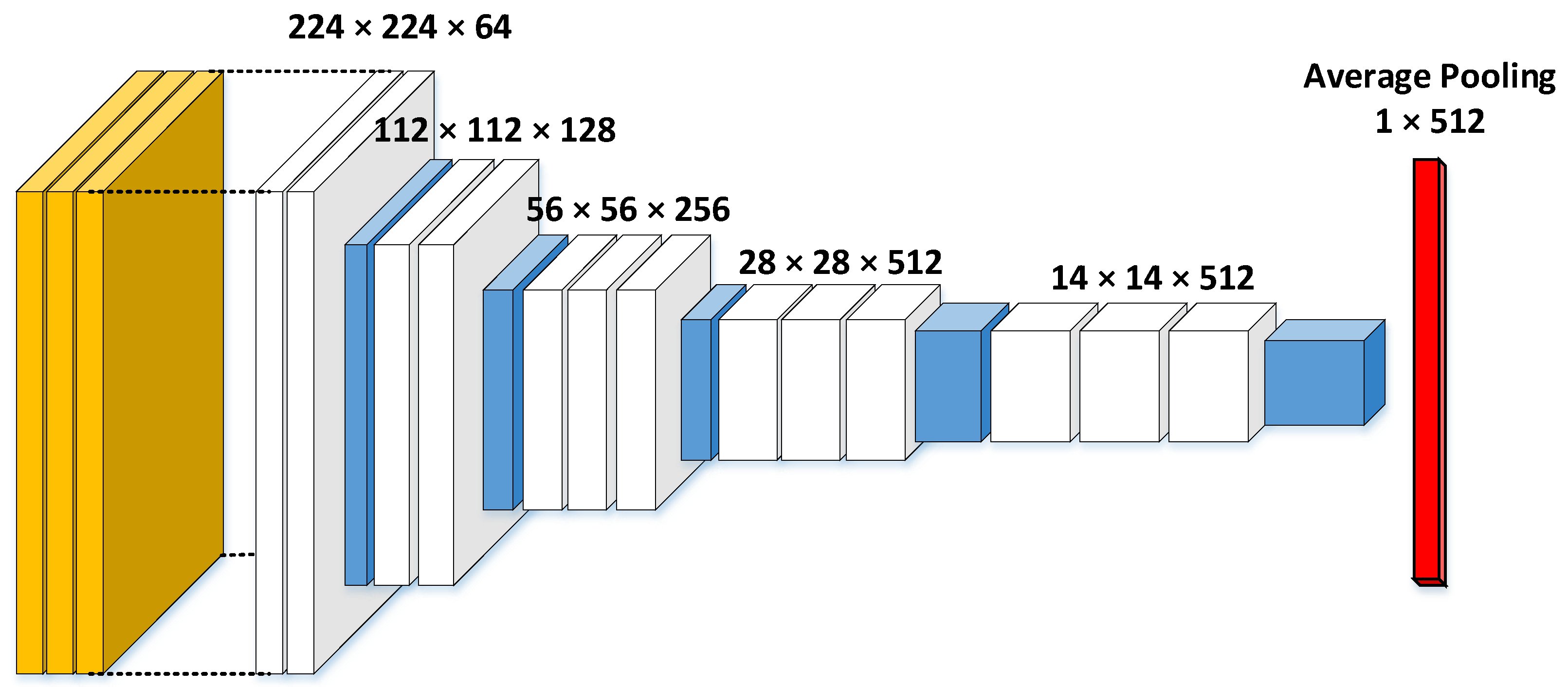
A basic CNN architecture consists of convolutional, pooling and fully connected layers. The convolutional layers generate feature maps by sliding automatically learned filters over input images. These feature maps are down-sampled by pooling layers, as indicated in Figure 1. Max-pooling is often used, in which the maximum value of the features in a local neighborhood is retained. In this way, the image is downscaled to reduce the number of weights with each layer. The final layers of the network are fully connected and relate the features generated by the preceding layers to the labels connected with the images.

Training of the networks is accomplished by means of stochastic gradient descent and back propagation. CNNs have fewer parameters to learn than equivalent fully connected neural networks and process data more efficiently. As a consequence, CNNs have become entrenched as state-of-the-art methods in a growing number of applications involving image processing [29].

Nonetheless, one of the major drawbacks of CNNs, is that their initial construction often require massive amounts of data and high-end computational resources. This problem can be circumvented by making use of CNNs that have been pretrained on data from different domains, such as the ImageNet database [30]. This process of deploying pretrained CNNs to data from domains other than on which it was trained is known as transfer learning.

Transfer learning is facilitated by the hierarchical representation of image features at different network depths. Visual inspection of such learned features revealed that the first layers respond to general image features, such as edges and different colors [31]. Deeper layers combine these features into the objects they are trained to identify. In mineral processing, transfer learning has been successfully applied to the monitoring of flotation froths [32,33], grinding circuits [19,34], ore texture analysis [35] and particle size distributions [36].

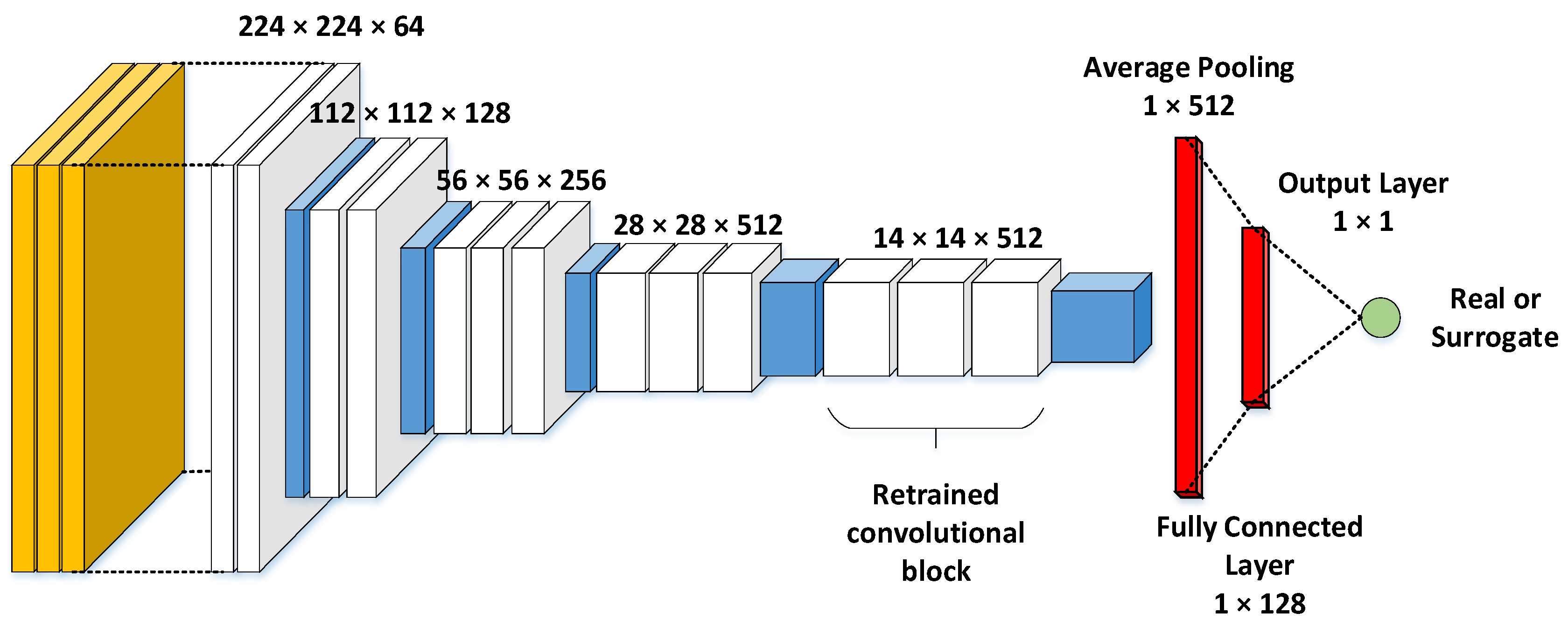
The architecture of VGG19 [37], the pretrained model used in this study, is shown in Figure 1. The shape of the feature maps output by each section of convolutional filters are shown. Images are presented to the model in RGB format. For a thorough discussion on CNNs and the various layers contained in the models, the reader is referred to Goodfellow et al. (2016) [29].

3. Dynamic Process Monitoring Methodology

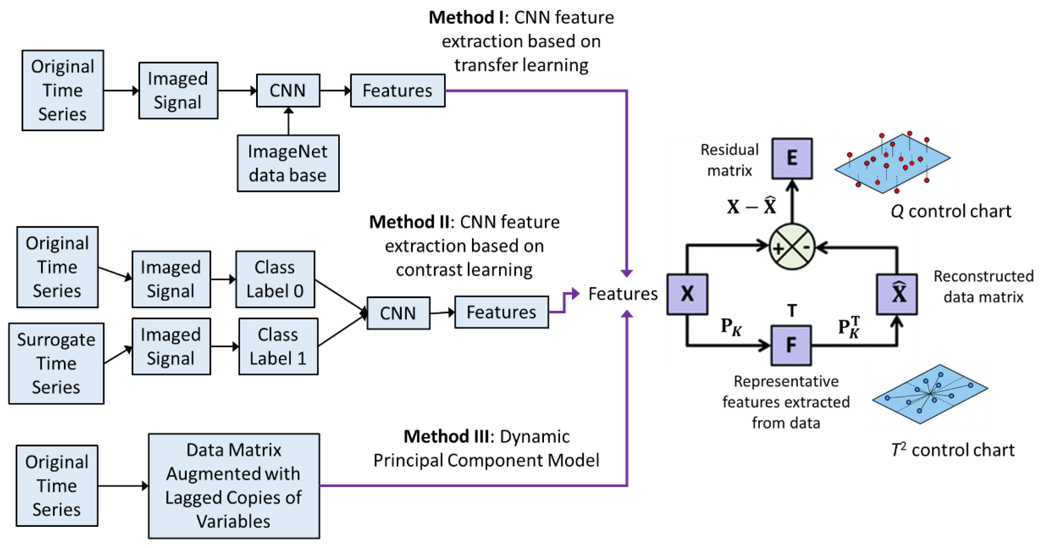
This section first describes the overall dynamic process monitoring framework, before a detailed description of each of the methodology based on the use of convolutional neural networks is given. Two variants of the methodology are considered, which are referred to as Methods I and II. In Method I, features are extracted through transfer learning only. In Method II, feature extraction is enhanced by use of an artificial classification problem that forces the CNN to extract features more descriptive of the data distributions. These approaches are compared with monitoring based on dynamic principal component analysis, which is referred as Method III, as described in more detail below.

3.1. Dynamic Process Monitoring Framework

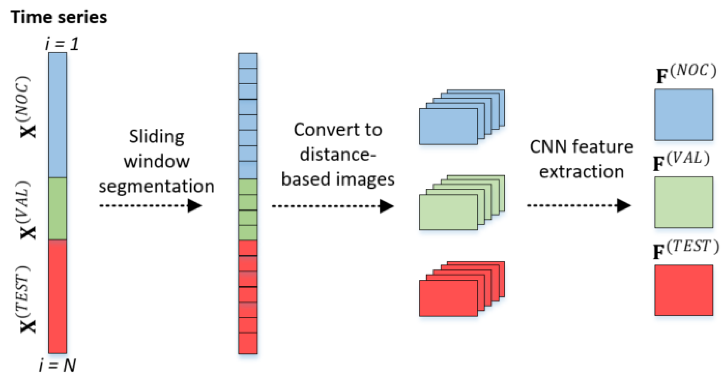
Time series data, $X\in {\mathbb{R}}^{N\times M}$, with N observations in M dimensions are divided into reference and test datasets, denoted $X^{\left(NOC\right)}$ and $X^{\left(TEST\right)}$, respectively. In practice, $X^{\left(NOC\right)}$ represents normal operating condition (NOC) data on which the monitoring algorithm is trained. $X^{\left(TEST\right)}$ represents new, unseen data which may or may not contain faults or process deviations. In contrast to $X^{\left(NOC\right)}$, $X^{\left(TEST\right)}$ is not available during the training stage of the model. As shown in Figure 2, $X^{\left(NOC\right)}$ is further subdivided into a validation set, $X^{\left(VAL\right)}$, to perform validation of the monitoring performance on data similar to $X^{\left(NOC\right)}$.

As mentioned above, both proposed monitoring approaches (Methods I and II) involve the extraction of features from segments of time series data. In both variants, the segmented time series data are transformed to images, and features are extracted from these images by use of a CNN. The feature matrices shown in Figure 2, $F$, are presented to a classical process monitoring scheme based on principal component analysis (PCA). The three methods considered in this investigation are summarized in Figure 3. Methods I–III are described in more detail in Section 3.2, Section 3.3 and Section 3.4, respectively.

After feature extraction, PCA is applied to $F^{\left(NOC\right)}$ to obtain the principal component loadings matrix, $P_K$. All three feature datasets are projected to the principal component space according to Equation (1), where K refers to the number of principal components retained to account for 90% of the variance in $F^{\left(NOC\right)}$.

$$T_K^{\left(TEST\right)}=F^{\left(TEST\right)}{P}_K^{\left(NOC\right)}$$

(1)

The principal component scores, $T_K$, calculated in Equation (1) are used to calculate Hotelling’s $T^2$-statistic, as defined in Equation (2).

$$T_K^2={\displaystyle \sum }_{i=1}^K\frac{t_i^2}{s_{t_i}^2}$$

(2)

where $t_i$ refers to column i of matrix $T_K$ and $s_{t_i}$ is the eigenvalue of the corresponding column in the PCA model. The data are projected back to the original feature space according to Equation (3):

$${\widehat{F}}_K^{\left(TEST\right)}=T_K^{\left(TEST\right)}{P}_K^{\left(NOC\right)}$$

(3)

allowing for the calculation of the $Q$-statistic, representing the reconstruction or Squared-Prediction-Error (SPE) of the model.

$$SP{E}^{\left(TEST\right)}={\displaystyle \sum }_{i=1}^R{(F_i^{\left(TEST\right)}-{\widehat{F}}_{K,i}^{\left(TEST\right)})}^2$$

(4)

where R refers to the number of samples in the feature matrix $F$. The monitoring performance of the PCA models are validated using the 95% confidence limits of the $T^2$ and Q statistics of the NOC data. These confidence limits are used as control limits on control charts, and an alarm is raised once these limits are exceeded, indicating a fault.

The performance of the algorithms was quantified by the true alarm rate (TAR), false alarm rate (FAR) and detection delay (DD). TAR is the fraction of detections flagged for known fault samples. FAR is the fraction of detections flagged on the validation dataset, which is known to be NOC data, i.e., the fraction of false positives. DD is defined as the number of consecutive known fault samples missed by the monitoring algorithm, before a detection is logged. For calculation of DD, detection was defined as three consecutive alarms.

3.2. Method I: CNN Feature Extraction Based on Transfer Learning

With Method I, sections of the time series were transformed into images and features were extracted from these images with a CNN making use of transfer learning. Any of a number of CNNs pretrained on the ImageNet database, can be used to accomplish this, but, in this investigation, the VGG19 CNN shown in Figure 1 was used.

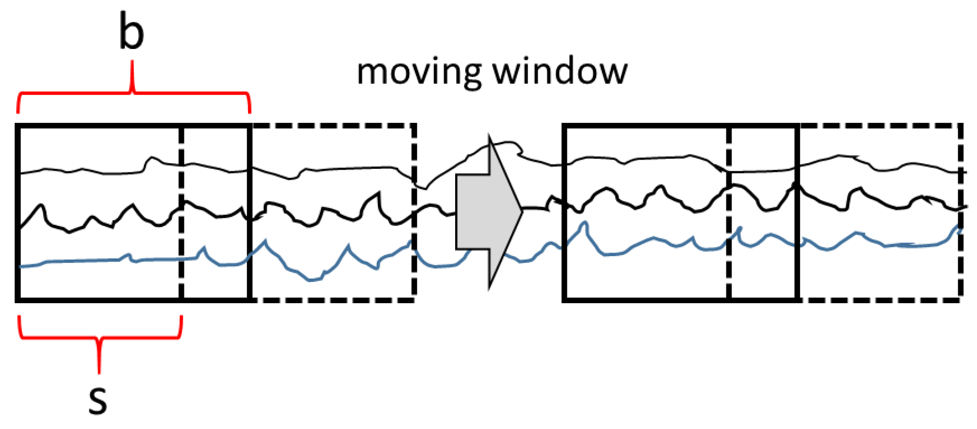
More formally, the zero mean, unit variance normalized multivariate time series data, $X\in {\mathbb{R}}^{N\times M}$ containing N measurements of M variables, were segmented by a moving window of length $b$, moving $s$ time steps at a time along the time series, as shown in Figure 4. In total, $R= floor\left(\frac{N-b+1}{s}\right)\in {\mathbb{R}}^{b\times M}$ such segments were constructed.

After segmentation of the time series, a distance matrix was constructed for each of the R time series segments. The elements of these distance matrices ($D_k\in {\mathbb{R}}^{b\times b}$) with elements $d^r\left(x_i,x_j\right), r=1,2, \dots R$ were the pairwise Euclidean distances between the points in the time series segment.

$$d^r\left(x_i,x_j\right)=\Vert x_i-x_j\Vert , for i,j=1,2,\dots ,b \& x_i,x_j\in {\mathbb{R}}^m$$

(5)

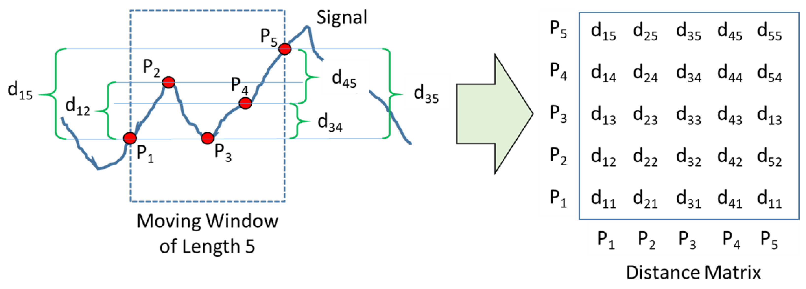
Figure 5 gives a diagrammatic representation of the calculation of a distance matrix in a window of length 5 sliding across a one-dimensional signal or time series. This gives a 5 × 5 distance matrix. Multivariate signals would be processed identically, with the distances computed in the corresponding multivariate Euclidean space. These distance matrices were presented directly to the convolutional neural networks, as equivalent to images, with the distance values equivalent to pixel intensities. These images can be considered a modified version of recurrence plots, as first proposed in [38]. Recurrence plots are a two-dimensional representation of the recurrences of state vectors in a dynamical system to local neighborhoods and are often used in the analysis of nonlinear or chaotic systems [39,40].

However, instead of confining the recurrence plot to returning trajectories in local neighborhoods, the thresholding function is removed to provide a global view of these trajectories in all neighborhood sizes. In this case, the different neighborhood sizes of the global recurrence plot (GRP) are represented as different colors in the image.

The feature extraction process is summarized in Figure 6. The distance matrices were presented to the CNN in the form of RGB color maps, instead of greyscale mappings.

The final classification layers of the VGG19 network were removed, since these layers are trained to classify images into the 1000 classes of common objects of the ImageNet dataset. As shown in Figure 1, the output of the final pooling block was downsampled and flattened using an average pooling layer. The layer reduces the output size to a 512-dimensional feature vector. Note that the output sizes in Figure 1 are given for the default image size of 224-by-224 pixels on which the network was trained. For a fixed-size convolutional filter, these output sizes change with the image size. In this work, the image size was dependent on the window length, $b$, and thus different intermediate output sizes were encountered; however, the number of feature maps remain constant, and the average pooling layer always results in a 512-dimensional vector. Implementation of the pretrained CNN models was facilitated by the Keras [41] and TensorFlow [42] libraries in Python.

In this first variant of the methodology, the CNNs pretrained on the ImageNet database were not trained any further, but simply used as feature extractors. These features, $F\in {\mathbb{R}}^{K\times n_F}$ with $n_F=512$ for the VGG19 CNN, were extracted for each of the NOC, validation and test datasets.

3.3. Method II: CNN Feature Extraction Based on Contrast Learning

Method II differs from Method I in that the pretrained networks were further trained to recognize the NOC data. An artificial training problem was set up to accomplish this. That is, in addition to the original time series, $X^{\left(NOC\right)}$, a surrogate time series was generated, $X^{\left(NOC\right)*}\in {\mathbb{R}}^{N\times M}$, with the same marginal distribution as the original time series, as well as the same autocorrelation function. This was accomplished by use of the iterated amplitude adjusted Fourier transform (IAAFT) algorithm [43].

The CNN was subsequently trained to distinguish between the real and surrogate data in a binary classification problem. Essentially, the original time series is masked or contrasted with the surrogate data, which forces the neural network to extract features that are descriptive of the distribution of the original NOC data, as it tries to discriminate between the two time series.

More formally, the surrogate time series was generated by an autoregressive moving average or Gaussian model of unidentified order. The IAAFT algorithm [43,44] used for this purpose can be summarized as follows:

(a)

Generate a sorted copy and random permutation of time series $X$, called $\tilde{X}$ and ${\mathit{S}}^{\left(0\right)}$, respectively.

(b)

Calculate the Fourier amplitudes of $X$ by the Discrete Fourier Transform (DFT):

$${\left|A_k\right|}^2={\left|\frac{1}{\sqrt{N}}{\displaystyle \sum }_{k=1}^N{X}_k{e}^{\frac{i2\pi }{N}kn}\right|}^2$$

(6)

(c)

The following steps are iterated until convergence:

(i)

Transform $S^{\left(i\right)}$ to the Fourier domain using DFT:

$$\mathcal{F}\left(S^{\left(\mathrm{i}\right)}\right)={\displaystyle \sum }_{k=1}^N{S}_k^{\left(i\right)}{e}^{-\frac{i2\pi }{N}kn}$$

(7)

(ii)

Generate $\widehat{\mathcal{F}}\left(S^{\left(\mathrm{i}\right)}\right)$ by replacing the Fourier amplitudes of $\mathcal{F}\left(S^{\left(\mathrm{i}\right)}\right)$ with ${\left|A_k\right|}^2$, while keeping the complex phases. This step ensures the original power spectrum is produced at each iteration.

(iii)

Take the inverse DFT back to the time domain:

$${\tilde{S}}^{\left(i\right)}=\frac{1}{\sqrt{N}}{\displaystyle \sum }_{k=1}^N\widehat{\mathcal{F}}{\left(S^{\left(i\right)}\right)}_k{e}^{-\frac{i2\pi }{N}kn}$$

(8)

(iv)

Generate $S^{\left(i+1\right)}$ by ranking the values of ${\tilde{S}}^{\left(i\right)}$ in ascending order and replacing them by the values of $\tilde{X}$ having the same ranking. Here, the distribution of the original series is retained.

(v)

Convergence is achieved once the ranked order of ${\tilde{S}}^{\left(i\right)}$ is identical to that of $\tilde{X}$, and ${\tilde{S}}^{\left(i\right)}$ is returned as the surrogate time series.

The original time series was labeled as 0 and the surrogate time series as 1. Both time series were segmented, and the segments were converted to GRPs, as was done with Method I. The labels associated with time series measurements were also mapped to the segments or corresponding images derived from the specific time series. These images and their associated labels were then concatenated into a single training database.

The classification section of the VGG19 network was modified to enable training to classify the real and surrogate data. Details of these modifications are summarized in

Table 1. Modified CNN architecture for contrast-based learning (Method II).

Layers	Output Shape	Description
VGG 19 pretrained feature extraction layers	$\left(w\times w\times 512\right)$	Feature map dimensions, $w$, dependent on window length
Global Average Pooling	$\left(1\times 512\right)$	Calculates average value over $w\times w$ feature map
Fully connected	$\left(1\times 128\right)$	128 nodes with Rectified Linear Units (ReLU) nonlinearity
Output node	$\left(1\right)$	Single output node with sigmoidal nonlinearity

and Figure 7. The output shapes given in the second column in Table 1 pertain to a single sample, corresponding to one segment of time series data of length $b$. The output of the sigmoidal nonlinearity in the final node distinguishes between the two classes.

Since the goal is improved feature extraction, the final section of convolutional filters were retrained, as indicated in Figure 7. Prior to retraining, this section outputs 512 feature maps, each of size $14\times 14$, trained to successfully characterize and predict the classes in the ImageNet dataset. After retraining, the convolutional filters generating these feature maps will have been repurposed to better identify the differences between the original and surrogate datasets considered here.

Once training is complete and the network can successfully discriminate between the original and surrogate data, the fully connected layers are removed. Features are again extracted for the $X^{\left(NOC\right)}$, $X^{\left(VAL\right)}$ and $X^{\left(TEST\right)}$ datasets similarly to the previous variant.

The difference between the features generated by Method II and those generated by Method I, is that, in the latter case, the features are solely derived from transfer learning from the ImageNet database. In Method II, the features are derived from contrast learning of the original time series data. In essence, the CNN is attempting to differentiate between the original time series and its surrogate mask. It accomplishes this by learning the decision boundary enclosing the features corresponding to the original NOC time series data. This decision boundary should enable not only distinguishing between original NOC data and surrogate data, but also NOC data and data from any other distribution, such as fault data.

For comparative purposes, process monitoring based on the use of dynamic principal component analysis is also considered, referred to as Method III, as discussed in the next section.

3.4. Method III: Dynamic Principal Component Analysis

Ku et al. [20] proposed a DPCA method using a time lag shift method in model building procedure. Since then, different variants of DPCA have been proposed to address different problems in industry. For example, Li and Rong [45] proposed the use of partial DPCA to obtain structured residuals and to improve the capability for fault isolation. Russel et al. [46] applied canonical variate analysis (CVA) statistics and DPCA for more sensitive fault detection. Dynamic kernel PCA was proposed by Choi and Lee [47] and Jia et al. [48], with further improvements proposed by Zhang et al. [22].

Principal component analysis can be extended to deal with dynamic process behavior by expanding the data matrix with time lagged copies of the variables [20]

$$\begin{array}{c}X=\{x_1\left(t\right),x_1\left(t-\ell \right),\dots x_1\left(t-\left(𝒹-1\right)\ell \right), x_2\left(t\right), x_2\left(t-1\right),\dots \\ x_2\left(t-\left(𝒹-1\right)\ell \right),\dots x_m\left(t-\left(𝒹-1\right)\ell \right)\}\end{array}$$

(9)

where $\ell$ is the embedding lag and $𝒹$ is the embedding dimension of the time series. In dynamic PCA models, the analyst needs to decide on the number of lags to add to each variable in addition to the number of principal components to retain in the model. Different approaches have been proposed for this, e.g., by taking into account the autocorrelational behavior of the time series [49] or the methods proposed by Rato and Reis [50], where a single lag structure ($\ell$) is determined for all the variables.

In this investigation, the objective was to detect change in the process system as rapidly as possible, so that the product of the embedding lag and the embedding dimension was minimized. For example, in a steady state system, with a lag of zero and embedding dimension of one, change can be detected as soon as a single sample on all the measurements that have been collected.

DPCA does not require analysis of segments of time series as the other two variants proposed. Instead, the time series embedded into a lag-trajectory matrix is input directly into the classical process monitoring scheme based on PCA, as shown in Figure 3.

4. Case Studies

4.1. Simulated Sinusoidal Dataset

4.1.1. Dataset Description

The analytical methodologies are demonstrated on a composite simulated signal generated by the combination of three sinusoidal signals and additive Gaussian noise, $\mathcal{N}\left(0,0.01\right),$ with zero mean and a standard deviation of 0.01, as indicated in Equation (10):

$$x\left(t\right)=\{\begin{array}{c}\sin \left(0.11t\right)+\sin \left(t\right)+0.1\sin \left(10t\right)+\mathcal{N}\left(0,0.01\right), t<1000\\ \sin \left(0.12t\right)+\sin \left(t\right)+0.1\sin \left(10t\right)+\mathcal{N}\left(0,0.01\right), t\ge 1000\end{array}$$

(10)

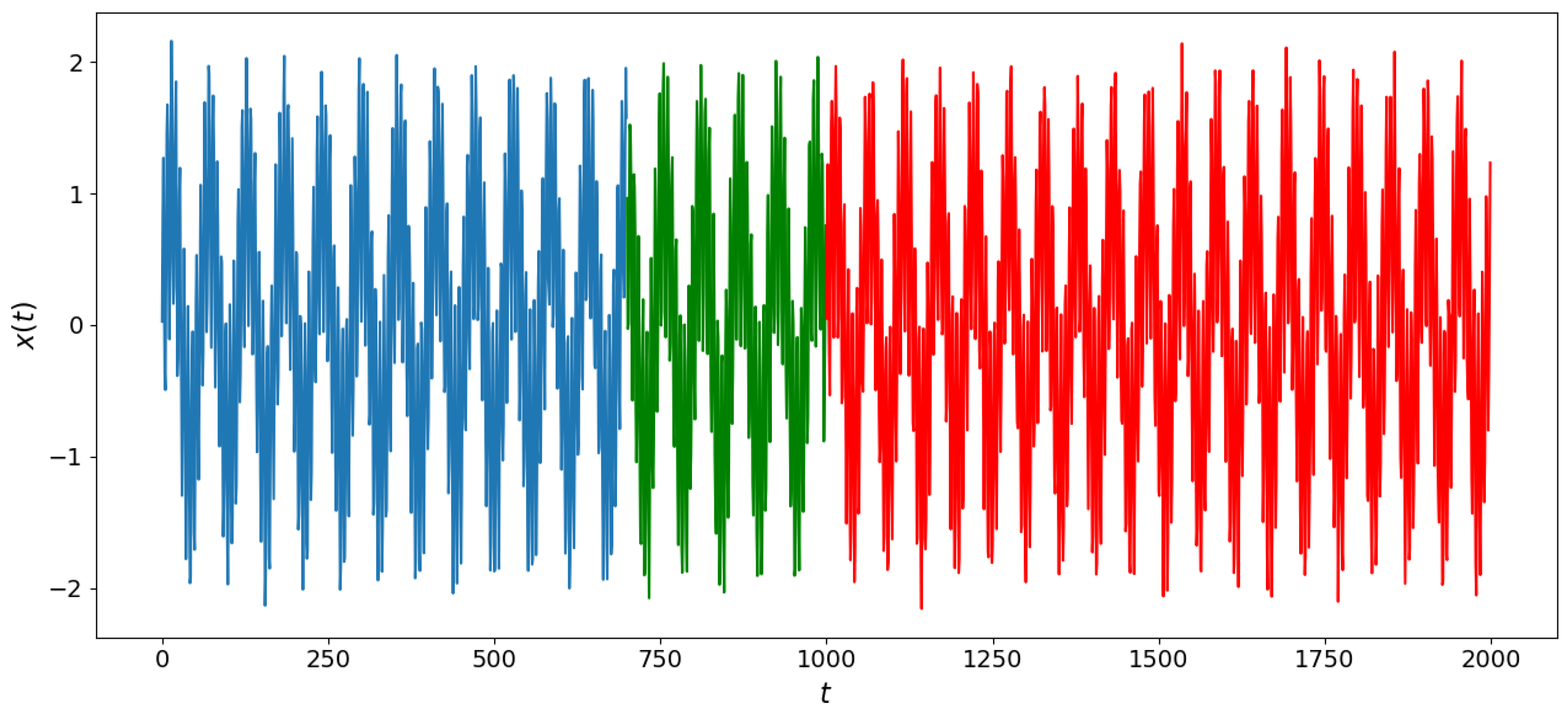
The signal was simulated for 2000 time steps, with the frequency of one of the sinusoidal components changing after 1000 time steps to mimic a fault. The simulated signal is depicted in Figure 8.

The first 1000 time steps were divided into NOC and validation data in a 70/30 ratio, with NOC data in blue and validation data in green. Test data, wherein the whole dataset contains the fault, is indicated in red. Figure 8 demonstrates that a visual inspection would not suffice to detect the parameter change. In the following sections, the process monitoring strategies described are applied to detect the parameter change in the time series.

4.1.2. Method I: CNN Feature Extraction Based on Transfer Learning

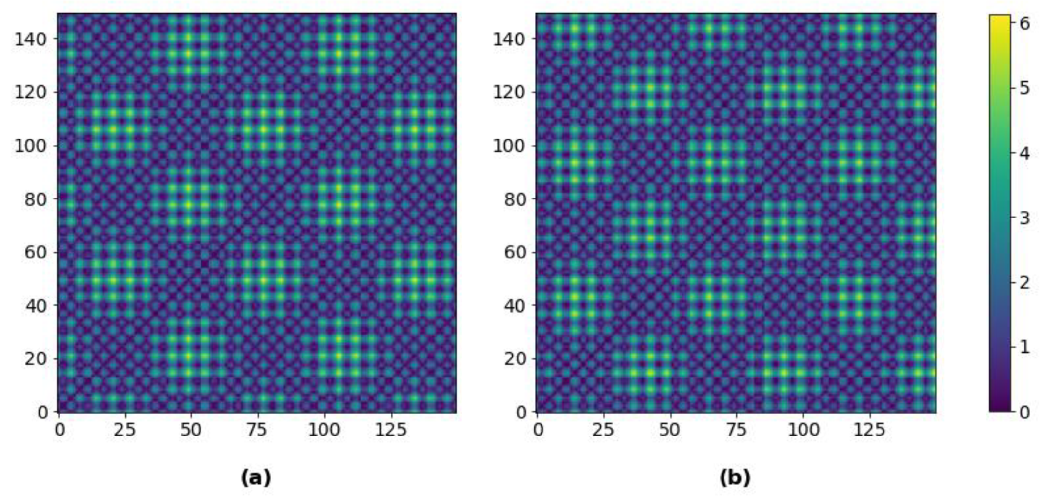
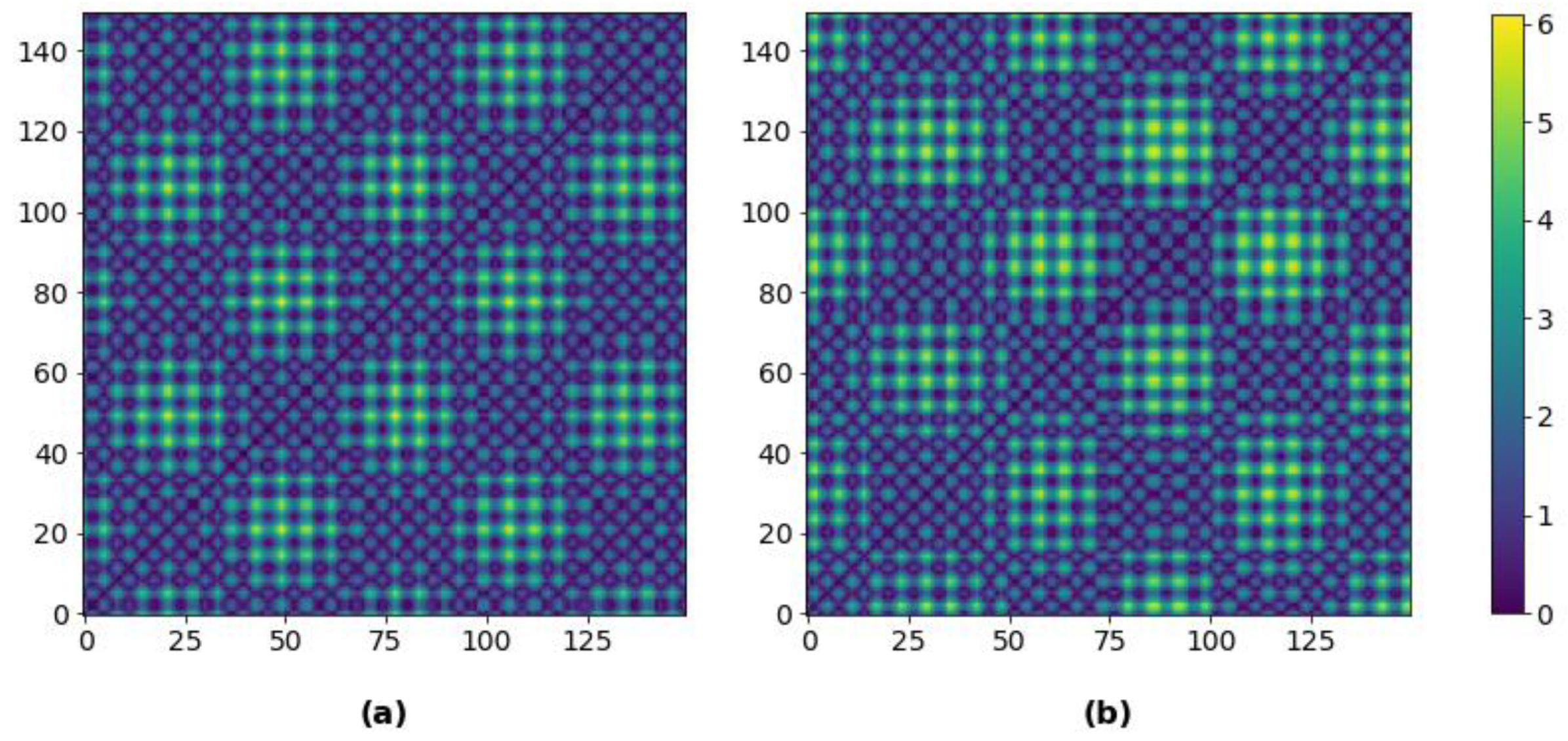
Methods I and II were both tested at four different window lengths. The stride between windows was maintained at a value of s = 1 to ensure the fault condition is detected as soon as possible. Examples of GRPs with a window length of 150 time steps are shown in Figure 9. As a final preprocessing step, the mean values of the RGB channels of the original ImageNet training dataset is subtracted from the GRP pixel matrices, to ensure that the pixel ranges of the images are similar to those the model was trained on.

After feature extraction, the principal component monitoring scheme was applied. The results in Figure 10 were used to determine the number of principal components to retain for monitoring calculations. The figure contains the cumulative sum of the normalized eigenvalues extracted from $F^{\left(NOC\right)}$, also for a window length of 150 time steps. For a window length of 150 time steps, 84 principal components were required to capture 90% of the variance in the $F^{\left(NOC\right)}\in {\mathbb{R}}^{K\times 512}$ feature matrix, as indicated in Figure 10.

The results for the simulations are summarized in

Table 2. Monitoring results on simulated dataset using Method I.

Window Length	FAR		TAR		DD
	${\mathit{T}}^{\mathbf{2}}$	Q (SPE)	${\mathit{T}}^{\mathbf{2}}$	Q (SPE)	${\mathit{T}}^{\mathbf{2}}$	Q (SPE)
50	0.063	0.035	0.062	0.076	15	16
100	0.044	0.052	0.288	0.280	10	10
150	0.047	0.031	0.481	0.487	24	24
200	0.033	0.042	0.537	0.623	23	20

. The TAR of both statistics increases with an increasing window length. The FAR in both cases approximates 0.05 (or 5%), as expected, since these data are similar to the NOC data from which the confidence limit was calculated. No clear patterns are observed in the detection delays, but the calculated values are short compared to the window lengths. According to the definition of the detection delay used, a minimum value of three time steps can be achieved. Overall, the best results were obtained with a window length of 200.

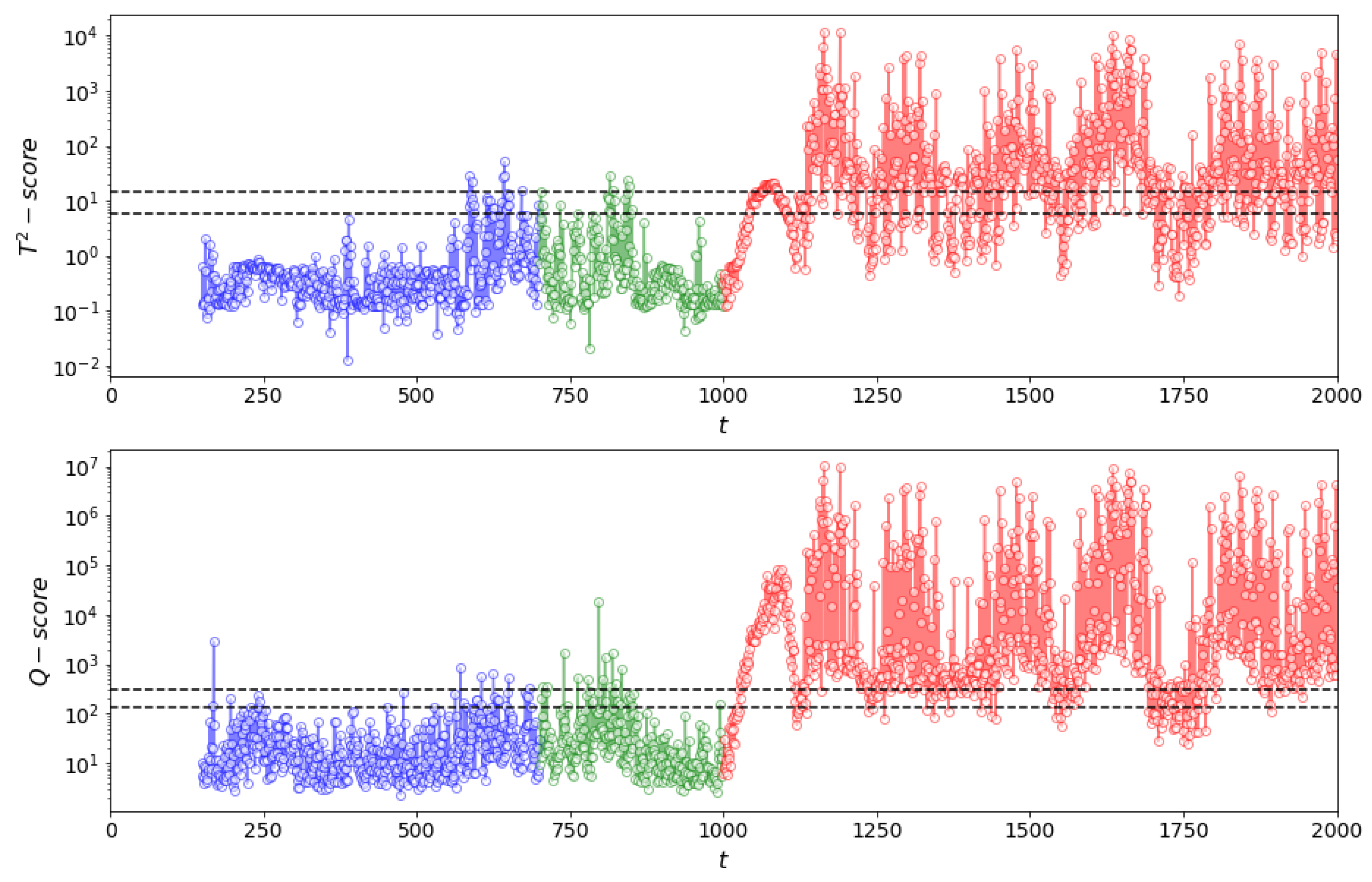
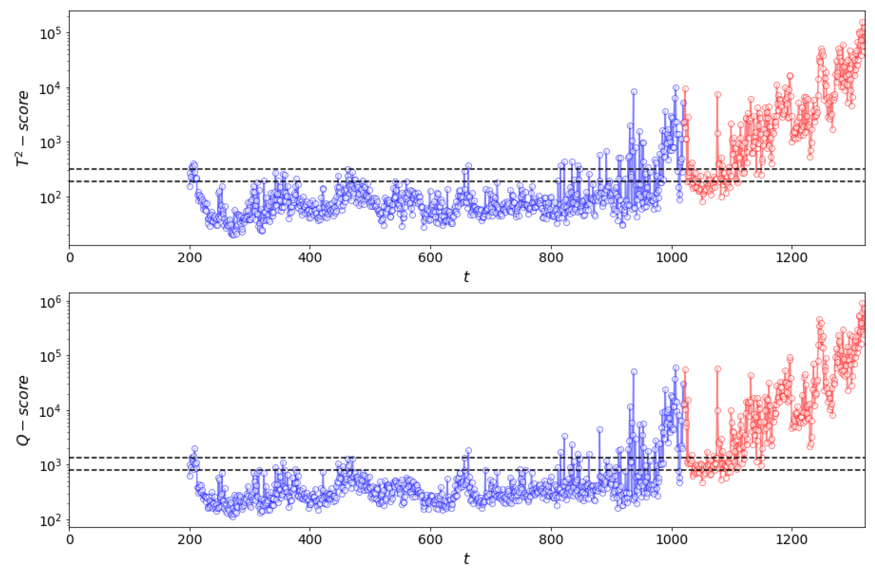
As an example, the $T^2$- and $Q$-statistic monitoring charts, for a window length of 150 time steps, are shown in Figure 11, with logarithmically scaled $T^2$- and $Q$-scores for better visualization. The 95% and 99% confidence limits are shown as broken lines. Note that the first value is plotted after 150 time steps, since the sliding window has to buffer until the window is fully populated before feature extraction can continue.

4.1.3. Method II: CNN Feature Extraction Based on Contrast-Based Learning

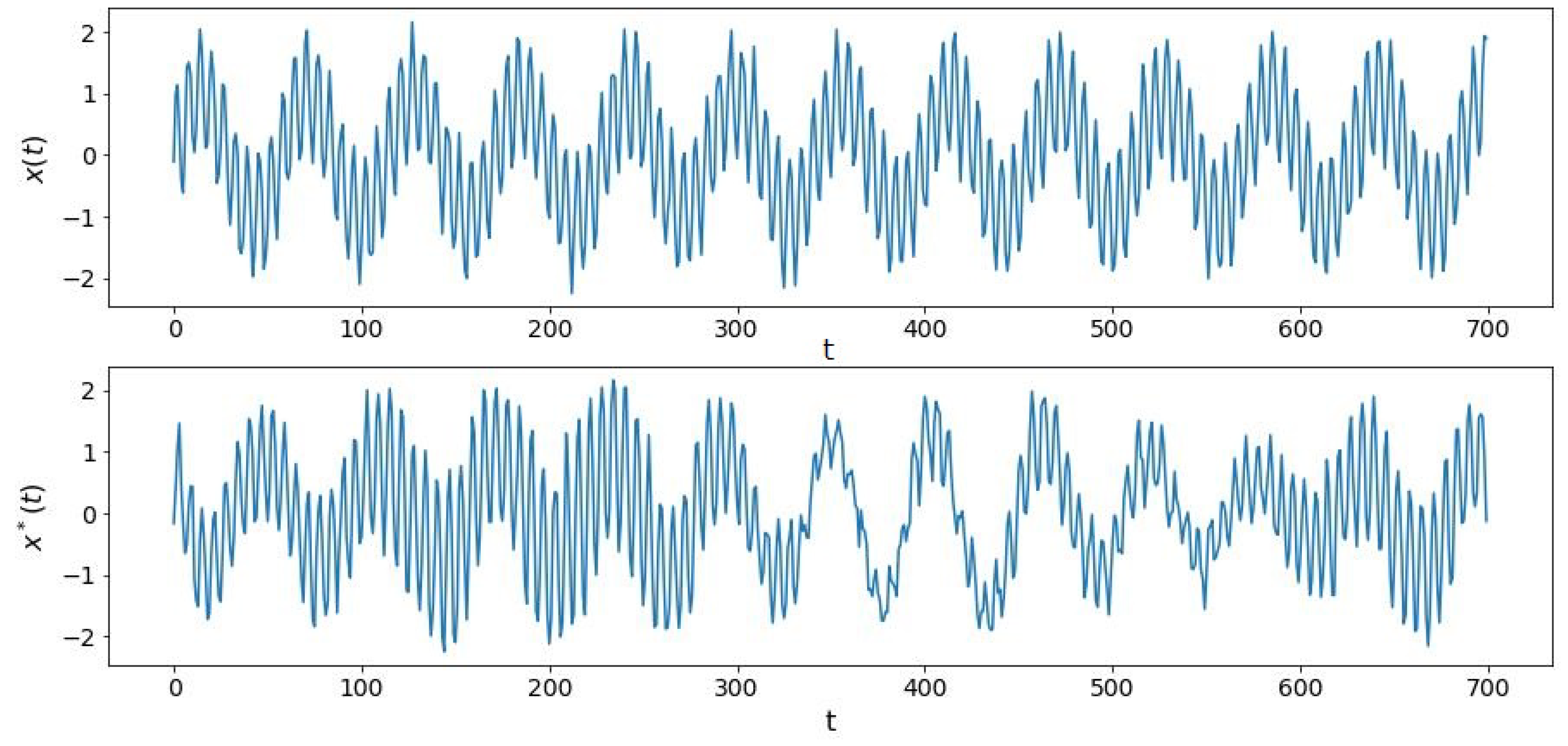
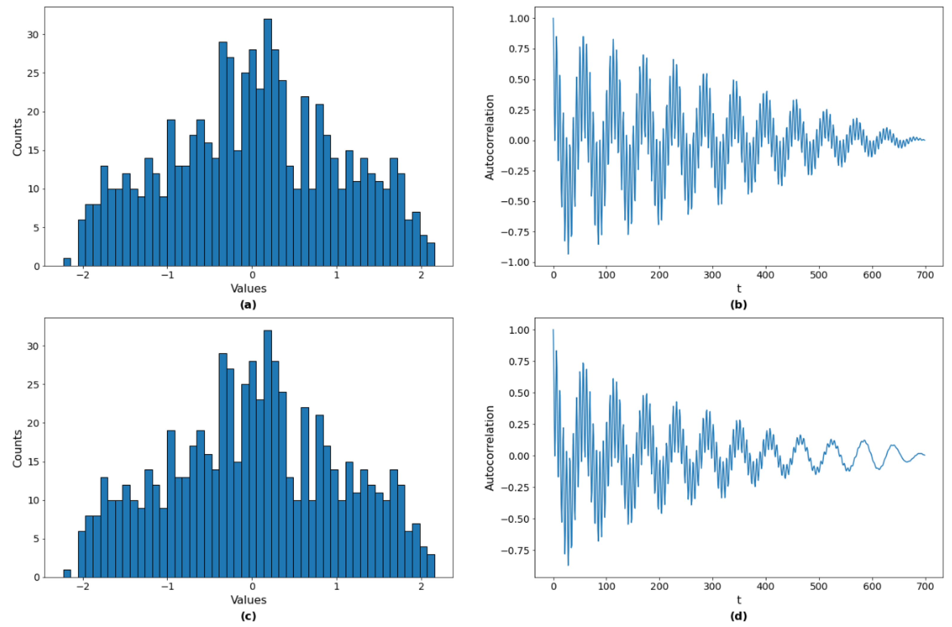
To enable contrast-based learning, an IAAFT surrogate of the simulated NOC data were generated, as shown in Figure 12. Figure 13 shows the distributions of the data in the two time series, as well as their autocorrelations functions. Examples of distance plots used during contrast-based training of the pretrained CNN are shown in Figure 14.

A CNN, with architecture as shown in Figure 7, was trained to classify the images using the parameters in

Table 3. CNN training parameters during contrast-based learning for Method II.

Parameter	Details
	Pretrain Newly-Added Classification Section	Fine-Tune Classification and Feature Extraction Sections
Loss function	Binary cross-entropy	Binary cross-entropy
Optimizer	Adam [51]	Adam [51]
Learning rate	0.01	0.0001
Training epochs	20	100

. The contrast-based learning procedure was achieved in two stages. Firstly, only the classification layers were trained with no alterations being made to convolutional filters. After 20 epochs through the training data, training of the final section of convolution filters commenced. The two-step procedure is required since the added classification layers were randomly-initialized and led to high loss function values in the first few epochs. These large losses result in high magnitude gradient updates to propagate throughout the network, causing large changes to filter weights and the benefit of using pretrained networks being lost. Thus, the initial training is necessary to reduce the loss function before changes to convolution filters are allowed. Further, a smaller learning rate is applied to the filter weights to prevent large weight adjustments resulting from slightly larger loss values. After training, the classification layers were removed, and features for NOC, validation and test data were extracted.

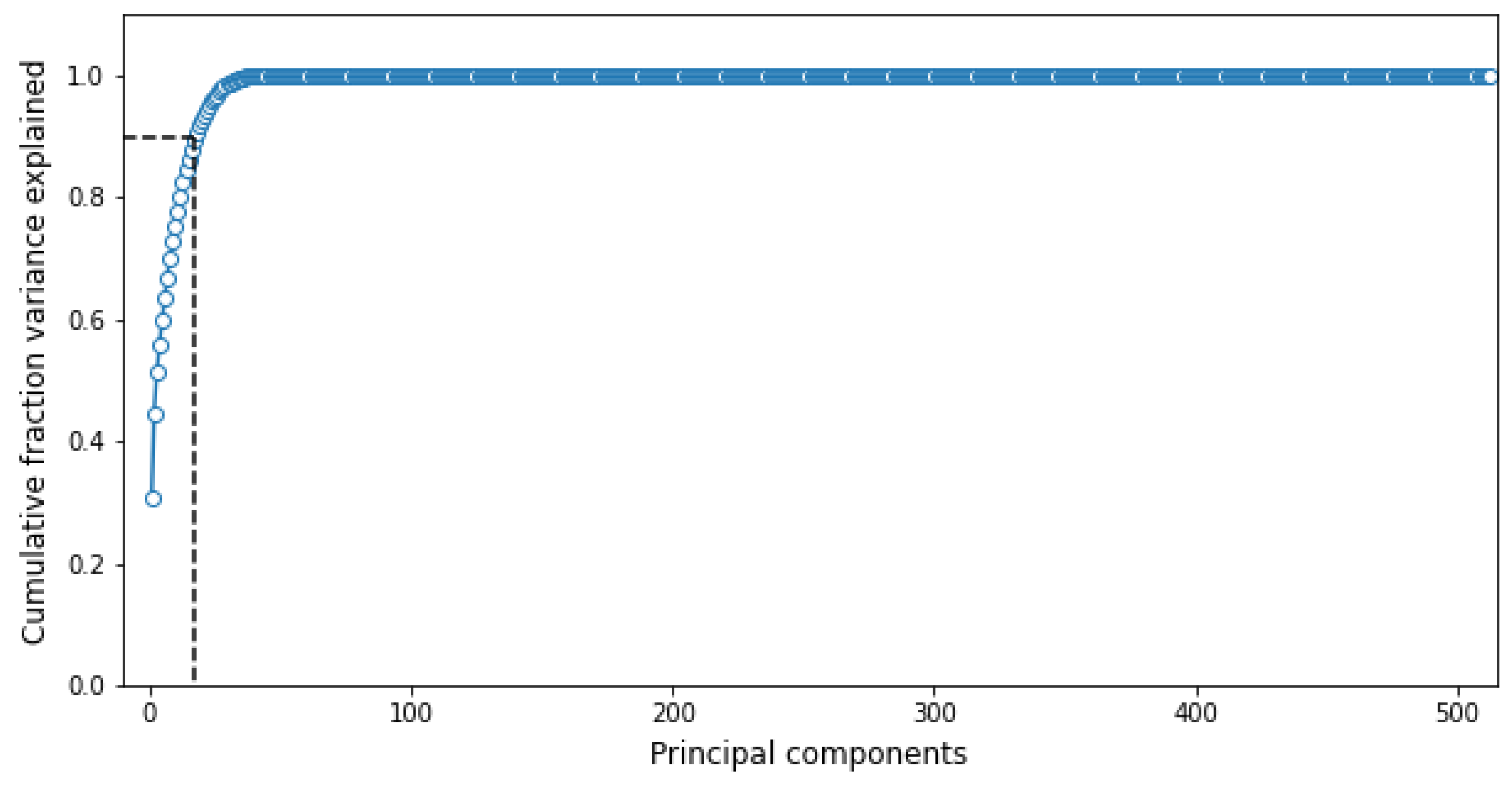
After feature extraction, the results in Figure 15 were used to determine the number of principal components to retain for monitoring purposes. Unlike the case with the first variant, only 17 principal components were required to capture 90% of the variance in the contrast-based learning features. Retraining the final section of convolutional filters adapted these filters to concentrate on discriminating between NOC and surrogate images, instead of properties of images in ImageNet dataset. Consequently, the network was able to extract a more compact feature set representing the variation in the NOC data.

The results of the monitoring simulations with different window lengths are given in

Table 4. Monitoring results on simulated dataset using Method II.

Window Length	FAR		TAR		DD
	${\mathit{T}}^{\mathbf{2}}$	Q (SPE)	${\mathit{T}}^{\mathbf{2}}$	Q (SPE)	${\mathit{T}}^{\mathbf{2}}$	Q (SPE)
50	0.050	0.050	0.109	0.142	13	13
100	0.010	0.003	0.322	0.392	15	14
150	0.013	0.040	0.849	0.880	41	31
200	0.113	0.123	0.415	0.341	3	9

. For similar window lengths, the contrast-based learning features improved monitoring performance over the transfer learning features, with the exception of the largest window length. The best result was found at a window length of 150 time steps, with the highest TARs and low FARs. The detection delay was however higher at this window length.

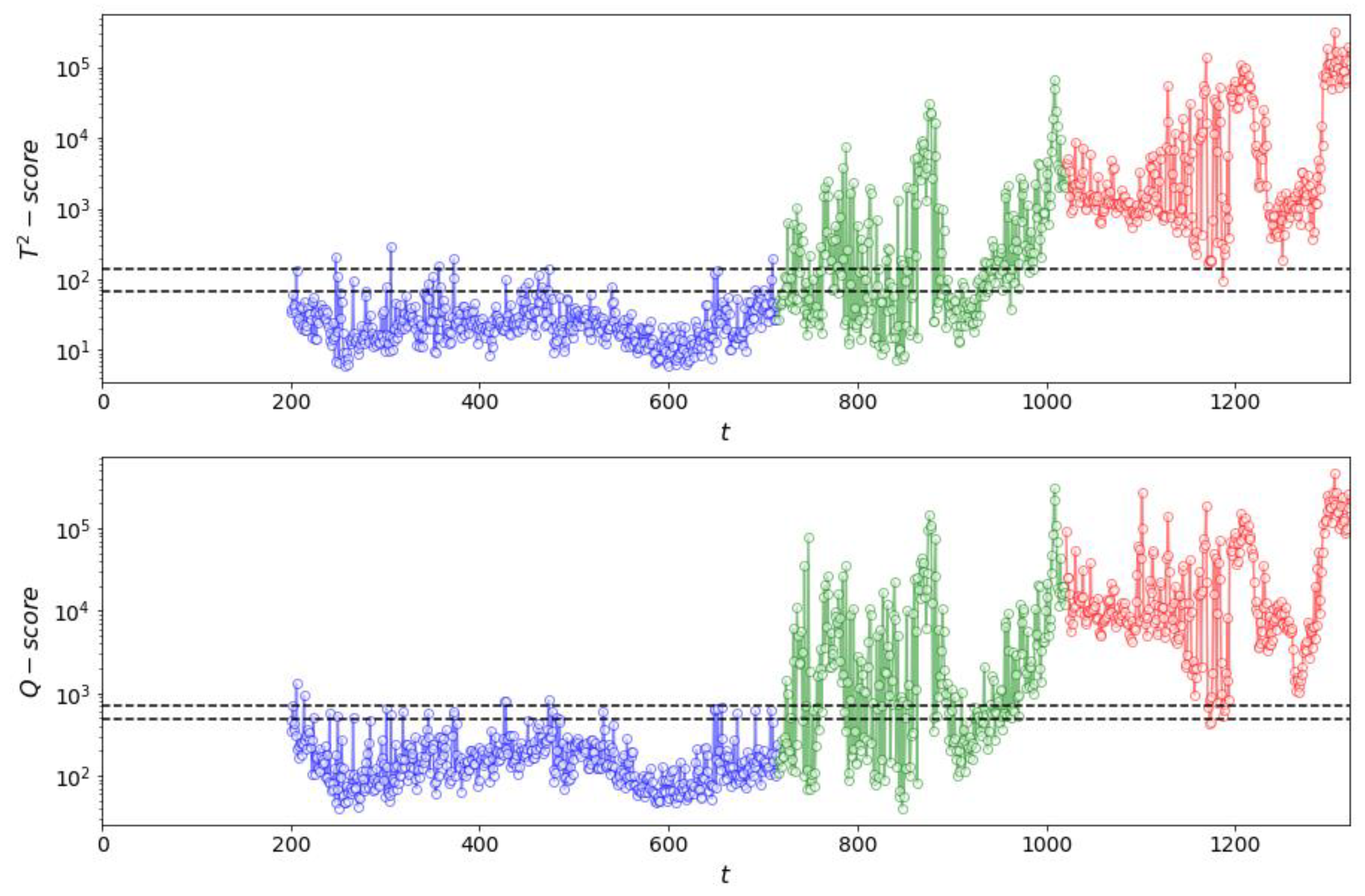
Again, the monitoring performance improved with window length, except for the largest window. The detection delay remains uncorrelated with the window length increase. The $T^2$- and $Q$-statistic monitoring charts, for a window length of 150 time steps, are shown in Figure 16. The $T^2$-values span a much lower range, since only 17 principal components are used during calculation, while the $Q$-scores are calculated on the remaining 495 principal components.

At the window length of 200, it is likely the decreased result is not because of the increase in length, but that training came to a halt while the filter weights were stuck in a suboptimal local minimum on the decision surface. Better results may have been found through longer training times, but overall it is clear that improved monitoring results can be obtained using contrast-based learning features over transfer learning features.

4.1.4. Method III: Dynamic Principal Component Analysis

DPCA results are dependent on the embedding lag and embedding dimension, according to Equation (9). For simulations, an embedding dimension was determined and results generated for a range of embedding lag values. Since the simulated signal consists of three components with added noise, an embedding dimension of four was chosen. The results are summarized in

Table 5. Monitoring results on simulated dataset using Method III with embedding dimension of four.

Embedding Lag	FAR		TAR		DD
	${\mathit{T}}^{\mathbf{2}}$	Q (SPE)	${\mathit{T}}^{\mathbf{2}}$	Q (SPE)	${\mathit{T}}^{\mathbf{2}}$	Q (SPE)
1	0.081	0.040	0.052	0.040	172	-
5	0.063	0.053	0.061	0.039	407	-
10	0.070	0.067	0.107	0.009	407	-
30	0.033	0.076	0.154	0.580	292	3
50	0.133	0.047	0.104	0.004	292	-

.

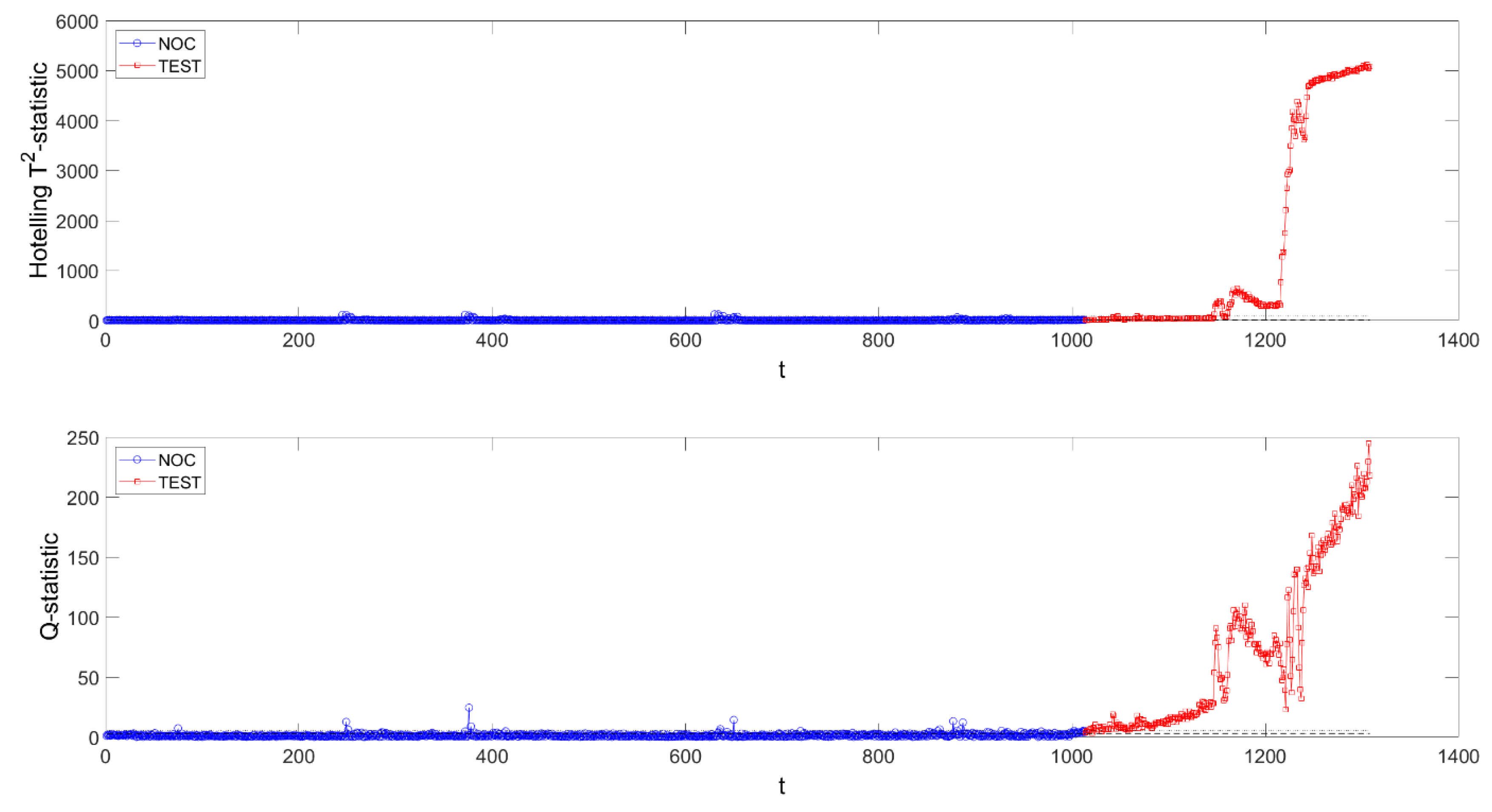
The sensitivity to the embedding parameters is clear from the results in Table 5. The only meaningful detection results were found at an embedding lag of 30. Monitoring charts for these parameters are depicted in Figure 17. On the simulated dataset, DPCA was outperformed by transfer learning features, while even more superior results were achieved when using features derived from contrast-based learning.

4.2. Monitoring the Power Draw of an Autogenous Milling Circuit

The process monitoring strategies encapsulated by Methods I–III were applied to an industrial autogenous grinding (AG) circuit on a platinum group metals concentrator. In this instance, the power draw of the AG mill was monitored, sampled at 5-s intervals. A change in the power draw generally implied a change in the mill load due to changing feed ores. Additionally, a fault was simulated in the data by gradually transforming the power draw data stream into white noise, as described by Equation (11).

$$x\left(t\right)=\{\begin{array}{cc}\hfill y\left(t\right),& t<1100\hfill \\ \hfill \left(1-\alpha \right)\times y\left(t\right)+\alpha \times y^{*}\left(t\right),& 1100\le t<1900\hfill \\ \hfill y^{*}\left(t\right),& t\ge 1900\hfill \end{array}$$

(11)

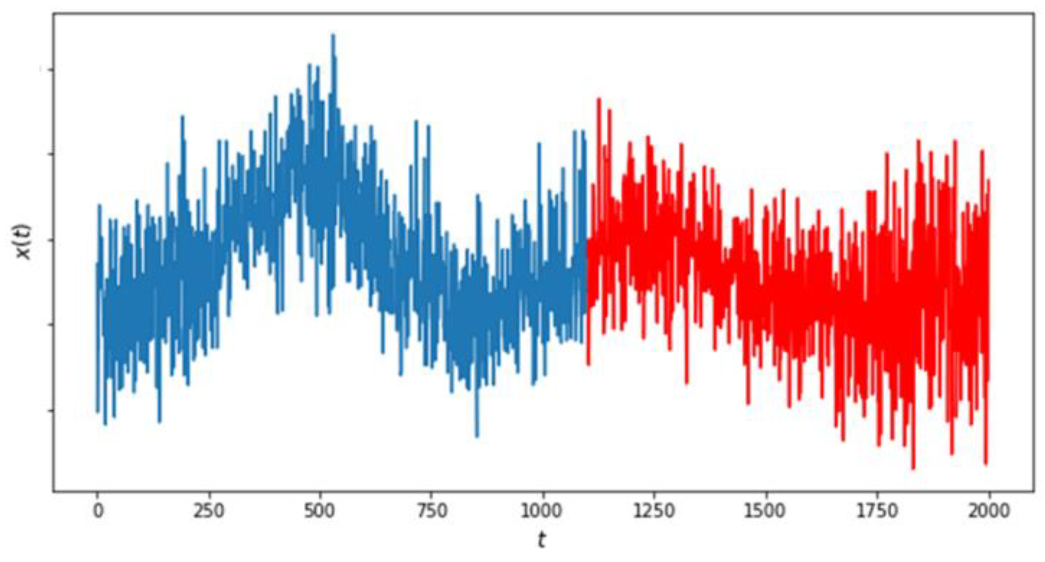
where $y\left(t\right)$ are the raw power draw data, $y^{*}\left(t\right)$ is a random permutation of $y\left(t\right)$ and $\alpha$ is a vector of evenly spaced values between 0 and 1. The power draw with simulated fault is shown in Figure 18.

Since this is in part a real dataset, the time series does not remain steady for long periods of time, and performance evaluation on a validation set necessarily leads to high FARs. Thus, the data are classified as “fault” or “non-fault” data, instead of NOC and test data. Only the true alarm rate and detection delay are used to quantify monitoring performance.

4.2.1. Method I: CNN Feature Extraction Based on Transfer Learning

Process monitoring results for detection of the fault in the mill power draw signal using CNN features extracted using transfer learning are shown in

Table 6. Monitoring results on AG mill power draw using Method I.

Window Length	TAR		DD
	${\mathit{T}}^{\mathbf{2}}$	Q (SPE)	${\mathit{T}}^{\mathbf{2}}$	Q (SPE)
50	0.061	0.067	78	79
100	0.163	0.173	20	20
150	0.350	0.392	50	50
200	0.758	0.777	3	3

.

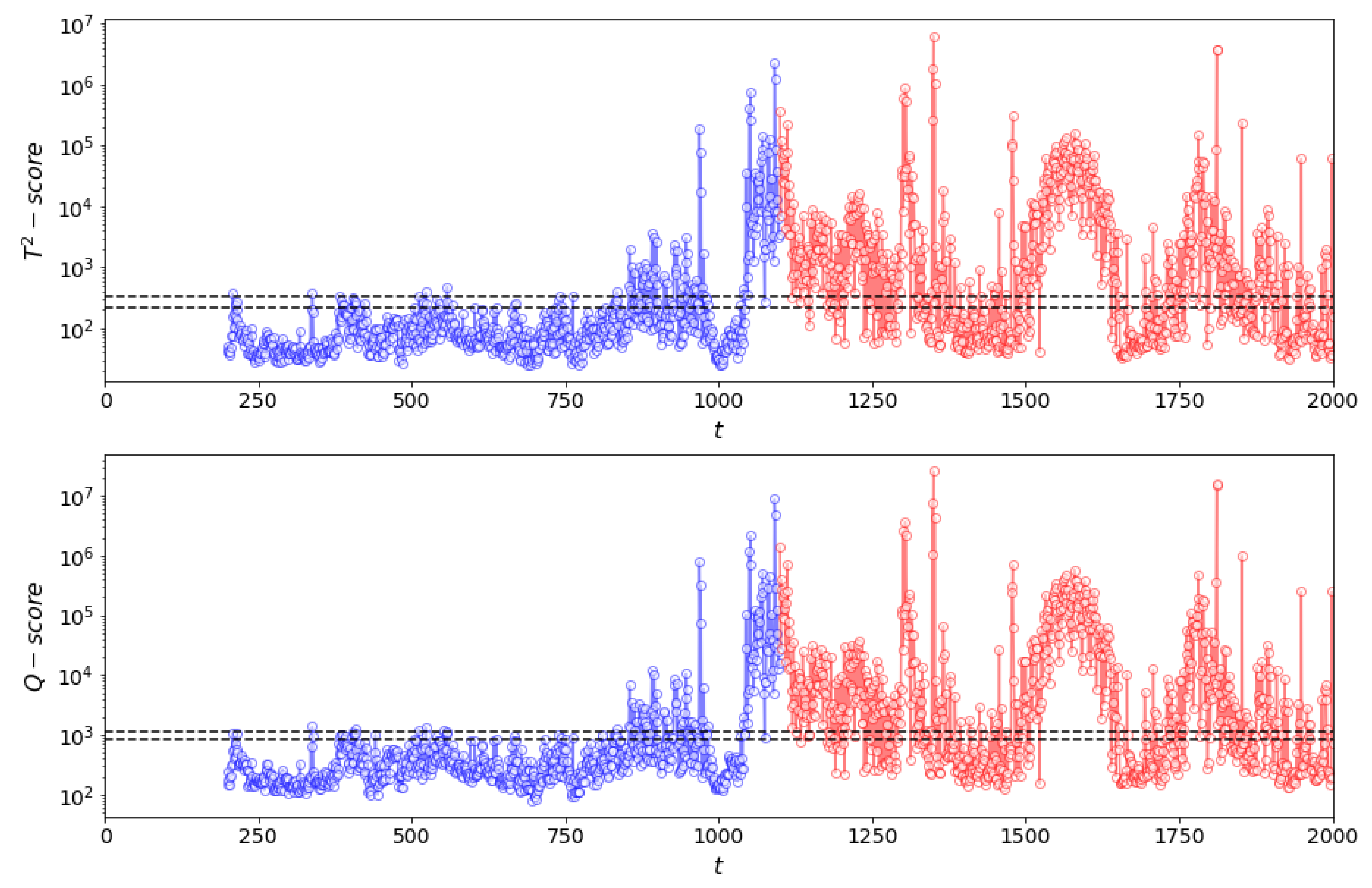
As before, the monitoring performance improves with an increasing window length, in terms of both the TAR and the detection time (DD) and the best performance is achieved at the largest window length of 200 time steps. The monitoring charts for this window length are shown in Figure 19.

4.2.2. Method II: CNN Feature Extraction Based on Contrast-Based Learning

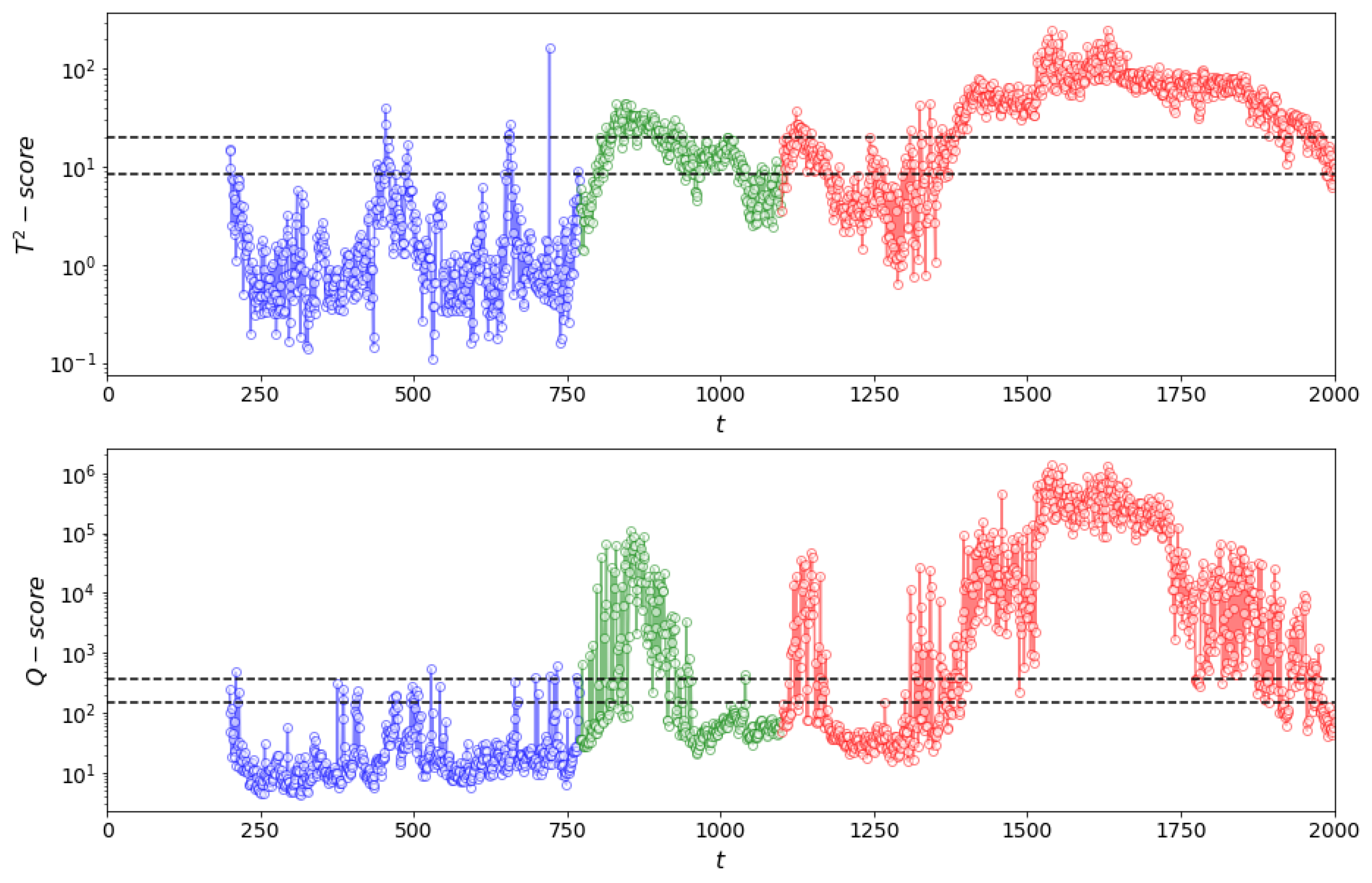
Process monitoring results for detection of the fault in the mill power draw signal using CNN features extracted through contrast-based learning are shown in

Table 7. Monitoring results on AG mill power draw using Method II.

Window Length	TAR		DD
	${\mathit{T}}^{\mathbf{2}}$	Q (SPE)	${\mathit{T}}^{\mathbf{2}}$	Q (SPE)
50	0.026	0.050	431	41
100	0.737	0.760	3	3
150	0.515	0.801	170	3
200	1.000	0.996	3	3

. The monitoring performance generally increases along with the window length, with the best results obtained at a window length of 200 time steps. At a window length of 50, the contrast-based training did not result in successful discrimination between the real and surrogate time series, leading to bad detection results. Monitoring charts at a window length of 200 are shown in Figure 20.

Figure 20 splits the non-fault data according to whether the data were seen by the model during contrast-based training. The data indicated by blue markers were seen during contrast-based learning, while the data indicated by green markers remained unseen.

Since the power draw signal was not steady over its duration, the unseen non-fault data are also flagged as faults. This could lead to the conclusion that the contrast-based learning procedure was simply overfitting the training data. However, this is countered by the low FARs achieved in Table 4 on the simulated data and the fact that the time series does not remain stationary during this period. Rather, the contrast-based learning features are correctly detecting that the time series is moving away from the training data. These results emphasize the sensitivity of the method to the training data. It is critical that a large dataset is used during training to capture the normal variation occurring during NOC periods.

4.2.3. Method III: Dynamic Principal Component Analysis

Process monitoring results for detection of the fault in the mill power draw signal using DPCA are shown in

Table 8. Monitoring results on AG mill power draw using Method III with embedding dimension of four.

Embedding Lag	TAR		DD
	${\mathit{T}}^{\mathbf{2}}$	Q (SPE)	${\mathit{T}}^{\mathbf{2}}$	Q (SPE)
2	0.0573	0.07645	-	776
5	0.0822	0.0792	797	-
10	0.0856	0.0907	791	805
30	0.0626	0.0484	-	819
50	0.0718	0.0588	803	-

. In the absence of knowing the true dimension of the underlying data generating distribution, the method of false nearest neighbors [52] was used to estimate the embedding dimension. The optimal embedding dimension was calculated to be four, where the number of false nearest neighbors decreased to zero. The monitoring simulations were run over a range of embedding lags, as seen in Table 6. Monitoring charts at an embedding lag of 10 time steps are shown in Figure 21.

The results show that DPCA was unsuccessful in detecting the simulated fault, or the movement of the unsteady time series data. Detection only occurs once the time series is close to fully consisting of white noise. This case study thus produces similar results to the first, with both Methods I and II performing better than Method III. Feature extraction based on contrast-based learning leads to additional superior monitoring performance above feature extraction based on transfer learning.

4.3. Monitoring the Operational State of an Autogenous Milling Circuit

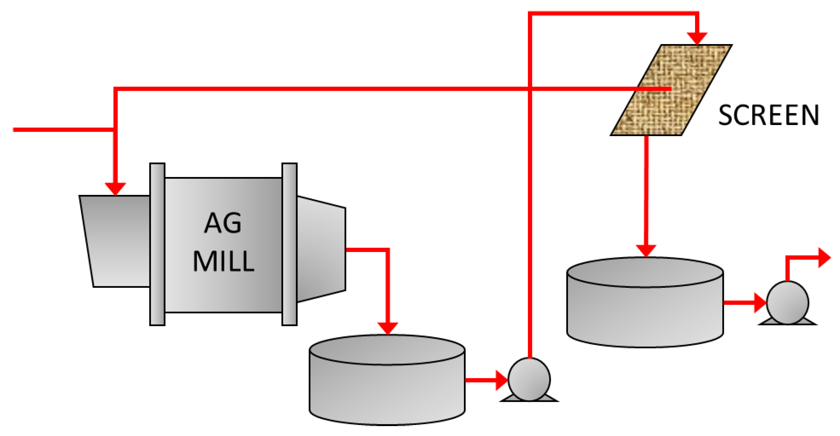
Multivariate data from an industrial grinding circuit were monitored for a change in the mill operational state. The grinding circuit consisted of a fully autogenous mill closed with a recirculating load originating from the oversize material of a screen. The grinding circuit is depicted in Figure 22.

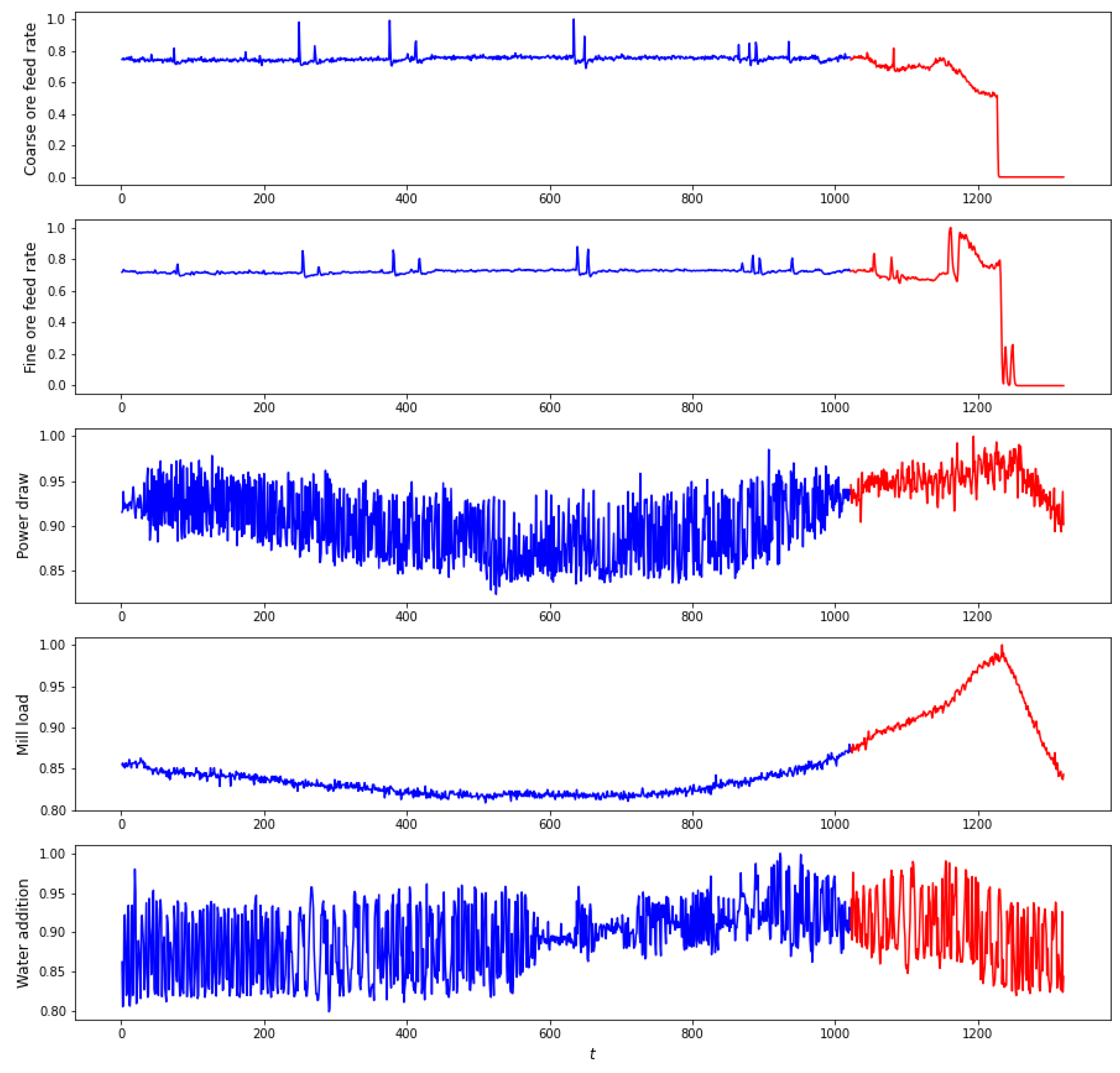
The monitored variables are the coarse ore feed rate, fine ore feed rate, mill power draw, mill load and the inlet water addition rate. Additionally, the milling circuit expert controller logged the operational state of the circuit at each sample, from a set of predefined states. The normalized samples of data collected at approximately 10 s intervals are shown in Figure 23.

For the samples considered, the mill gradually drifts from NOC to an overloaded state. The color change in Figure 23 corresponds to the exact time the expert controller identified the change in operational state. Such a change would generally result from a change in the feed ore competency or particle size distribution. The expert controller takes delayed corrective action by dropping the feed rates to return the circuit to a NOC state.

In the following sections, the monitoring methodologies are applied to the dataset to detect this change of operational state.

4.3.1. Method I: CNN Feature Extraction Based on Transfer Learning

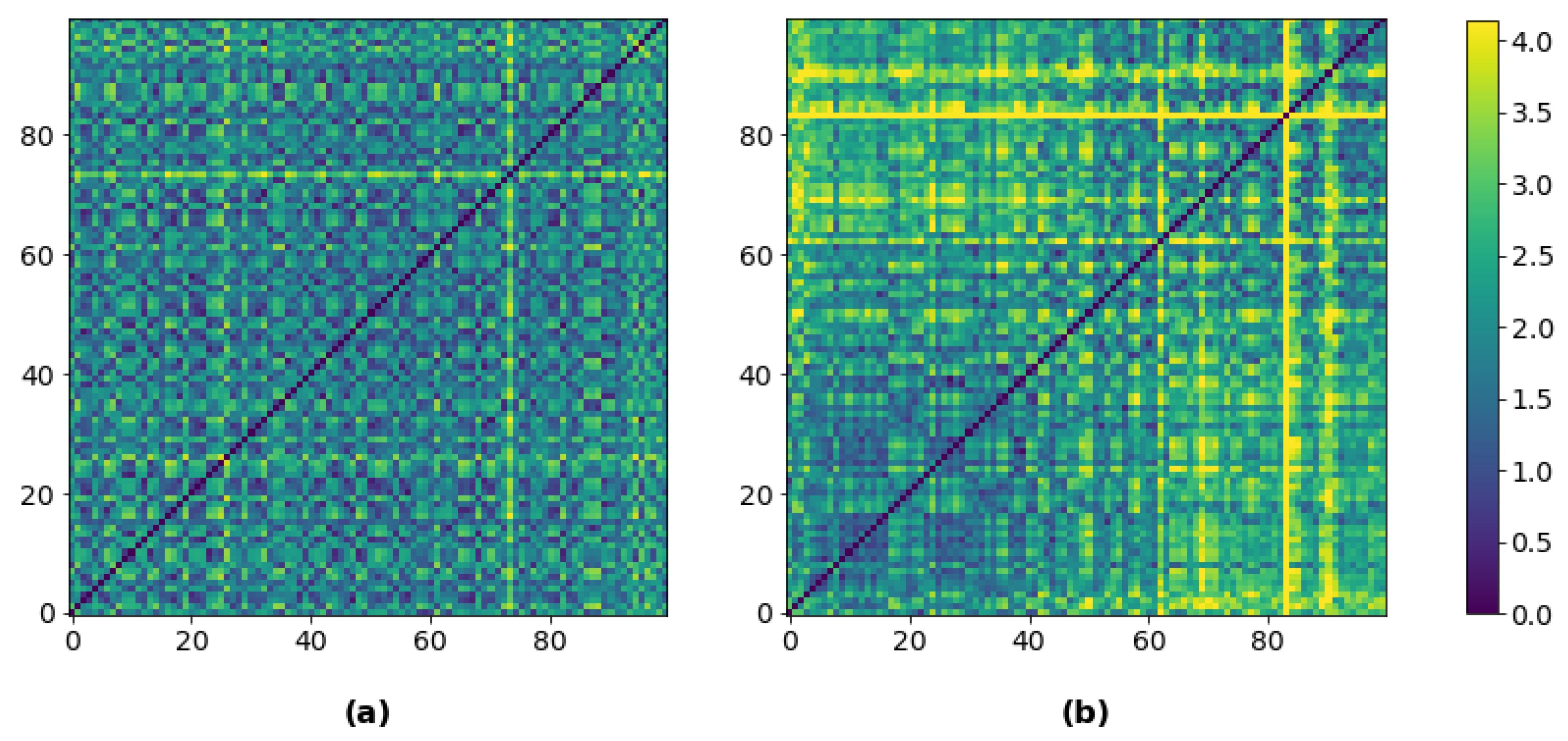
In this case study, the three methods are applied to multivariate time series data. Distance plots of the multivariate time series data for the NOC and overloaded mill state are shown in Figure 24.

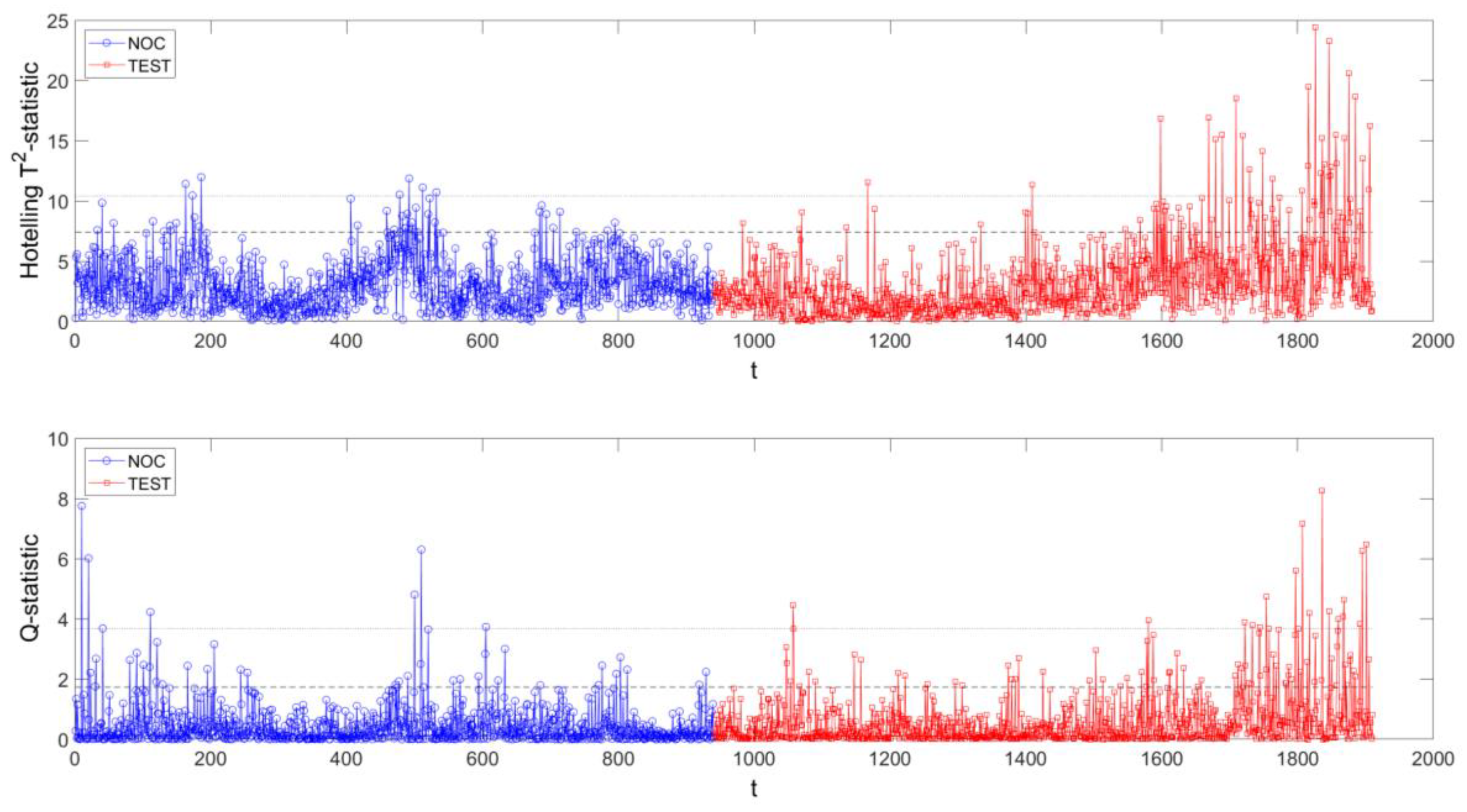
The results of the monitoring simulations are summarized in

Table 9. Monitoring AG mill operational state using Method I.

Window Length	TAR		DD
	${\mathit{T}}^{\mathbf{2}}$	Q (SPE)	${\mathit{T}}^{\mathbf{2}}$	Q (SPE)
50	0.723	0.753	3	3
100	0.965	0.975	3	3
150	0.820	0.870	62	34
200	0.900	0.937	3	3

. Again, the monitoring performance is only validated on the TAR and DD, since the circuit is not completely steady during the NOC period. Table 9 shows good detection results, with high TARs and short detection delays. Monitoring charts at a window length of 200 time steps are shown in Figure 25. From the charts, it appears the algorithm would identify the change in operational state slightly more quickly than the predefined control limits given to the expert controller.

4.3.2. Method II: CNN Feature Extraction Based on Contrast-Based Learning

For the multivariate case, a surrogate matrix was generated by first creating a surrogate for each individual time series. These surrogates were concatenated to form a surrogate matrix with the same shape as the original multivariate series. While the distribution and autocorrelation of each individual variable could be retained, any cross-correlation between variables are destroyed during surrogate creation.

The results of the monitoring simulations are summarized in

Table 10. Monitoring AG mill operational state using Method II.

Window Length	TAR		DD
	${\mathit{T}}^{\mathbf{2}}$	Q (SPE)	${\mathit{T}}^{\mathbf{2}}$	Q (SPE)
50	0.610	0.797	3	3
100	1.000	0.990	3	3
150	0.553	0.497	3	3
200	1.000	1.000	3	3

, and monitoring charts at a window length of 100 time steps are depicted in Figure 26. Again, NOC data not used for contrast-based training are displayed in green.

Better results were generally achieved using contrast-based learning features than could be achieved using transfer learning features, except at the window length of 150. At this window length, it is likely that training halted with the network weights stuck in a suboptimal local minimum. Additionally, it seems the trend towards the overloaded state is detected earlier and more pronounced than with transfer learning features.

4.3.3. Method III: Dynamic Principal Component Analysis

For DPCA, the lag-trajectory embedding of the multivariate time series was determined using the method of false nearest neighbors and the average mutual information criterion [53]. For each variable, the dimensions in which false nearest neighbors tend to zero, as well as the lag value at which the average mutual information criterion reaches a first minimum value, was calculated. The maximum of calculated embedding dimensions, as well as maximum time lag value, was used to embed all of the variables in the time series. This maximum dimension was two, with a maximum time lag of four time steps. Thus, the embedding resulted in a 10-dimensional matrix, two dimensions per variable, with time lags of four time steps between dimensions of the same variable.

The monitoring results are summarized in

Table 11. Monitoring AG mill operational state using Method III.

Embedding Dimension/Lag	TAR		DD
	${\mathit{T}}^{\mathbf{2}}$	Q (SPE)	${\mathit{T}}^{\mathbf{2}}$	Q (SPE)
2/4	0.993	1.000	6	3

and displayed in monitoring charts in Figure 27. The simulation was only run with one set of embedding parameters.

In this case, the DPCA model successfully detects the change in operational state, performing similarly to the CNN feature models. Visual inspection of the time series data in Figure 23 confirms that this detection is more trivial than the previous case studies. However, it still serves as a demonstration of the application of the methods to a multivariate problem.

5. Discussion

Convolutional neural networks were used to capture the structure of dynamic process variables in the form of sets of features that are representative of the time series behavior or process dynamics. The time series were encoded as a series of images from which features can be extracted via these networks. It is not technically necessary to convert the time series into images, as CNNs can take input of any dimension, including the time series directly.

However, conversion of the time series to images allows the user to exploit the use of pretrained CNNs that are available in the public domain, as has been done in a growing number of examples in a variety of applications [54,55]. Imaging of time series is advantageous for two reasons. First, it saves on the development cost (training time) of the CNNs, which can be considerable, and, second, it also allows the use of these models in the absence of the large datasets typically required in the development of CNN models. Mathematical transformation of the data might also reveal certain temporal correlations or interactions between variables that would otherwise be more difficult through analysis of the raw time series data. The method is easily extended to analysis of images generated from time-frequency—or multiscale transforms commonly used to analyze high frequency sensor data.

More specifically, the CNNs used in this investigation, and in a large number of other applications discussed in the literature, were trained on the ImageNet database of common objects. As a consequence, transfer learning can be used to generate features from other image datasets, as was done in Method I as applied to the case studies considered in this paper.

As informative as these features are, in principle at least, they are not necessarily optimal, especially if the images from the training and application domains are very different. Additional training could therefore go a long way towards further optimization of the features. With Method II, this is accomplished by setting up an artificial binary classification problem by generating synthetic data similar to the original data. Further training of the CNN to discriminate between these data in effect forces it to develop an internal set of features that are more specifically representative of the data in the application domain.

The efficacy of this approach is epitomized by the more compact set of features required to represent the data, as well as the comparatively favorable results that were obtained within the dynamic monitoring framework.

Both Methods I and II can be optimized in a number of ways. For example, imaging of the data based on Euclidean distance matrices may not be effective when the data lie on the convoluted low-dimensional manifold of a nonlinear dynamic system, but this could in principle be accounted for by use of more appropriate distance measures or different approaches to imaging of the data [56].

6. Conclusions

As shown in this investigation, convolutional neural networks can be used in dynamic process monitoring schemes where the time series measurements are converted to images. Two variants were proposed, based on the use of a pretrained CNN (VGG19). In the first (Method I), the network was used to extract features from data contained in a sliding window, by making use of transfer learning, which were further analyzed by a principal component model in a classical multivariate statistical process monitoring framework.

The second approach (Method II) was similar, except that the network was trained via an artificial classification problem to derive features that were more descriptive of the data. Both models performed better than a dynamic principal component model (Method III), although Method I did so only marginally, while Method II appeared to do so with a more significant margin.

Methods I and II would need to be validated further against additional case studies in different systems, but, as indicated in the previous section, there would be considerable scope for further optimization in among others, the CNN model used, the generation of images from the data and by extending the overall scheme to accommodate multiscale approaches.

References

1. Wei, D.; Craig, I.K. Grinding mill circuits—A survey of control and economic concerns. Int. J. Miner. Process. 2009, 90, 56–66. [Google Scholar] [CrossRef]
2. Muller, B.; De Vaal, P.L. Development of a model predictive controller for a milling circuit. J. South. Afr. Inst. Min. Metall. 2000, 100, 449–453. [Google Scholar]
3. Chen, X.S.; Zhai, J.Y.; Li, S.H.; Li, Q. Application of model predictive control in ball mill grinding circuit. Miner. Eng. 2007, 20, 1099–1108. [Google Scholar] [CrossRef]
4. Botha, S.; le Roux, J.D.; Craig, I.K. Hybrid non-linear model predictive control of a run-of-mine ore grinding mill circuit. Miner. Eng. 2018, 123, 49–62. [Google Scholar] [CrossRef] [Green Version]
5. Chen, X.; Zhai, J.; Li, Q.; Fei, S. Fuzzy logic based on-line efficiency optimization control of a ball mill grinding circuit. In Proceedings of the Fourth International Conference on Fuzzy Systems and Knowledge Discovery, Haikou, China, 24–27 August 2007. [Google Scholar] [CrossRef]
6. Gomez, A.; Aracena, C.; Cornejo, F.; Festa, A.; Vasquez, A. Rule and fuzzy-logic based expert control of Barrick Lagunas Norte mine. Automining 2010. In Proceedings of the 2nd International Congress on Automation in the Mining Industry, Santiago, Chile, 10–12 November 2010. [Google Scholar]
7. Van Drunick, W.I.; Penny, B. Expert mill control at AngloGold Ashanti. J. South. Afr. Inst. Min. Metall. 2005, 105, 497–506. [Google Scholar]
8. Inapakurthi, R.K.; Miriyala, S.S.; Mitra, K. Recurrent neural networks based modelling of industrial grinding operation. Chem. Eng. Sci. 2020, 219, 115585. [Google Scholar] [CrossRef]
9. Aldrich, C.; Burchell, J.J.; De, J.W.; Yzelle, C. Visualization of the controller states of an autogenous mill from time series data. Miner. Eng. 2014, 56, 1–9. [Google Scholar] [CrossRef]
10. Chen, X.S.; Li, Q.; Fei, S. min Supervisory expert control for ball mill grinding circuits. Expert Syst. Appl. 2008, 34, 1877–1885. [Google Scholar] [CrossRef]
11. Chen, X.; Li, S.; Zhai, J.; Li, Q. Expert system based adaptive dynamic matrix control for ball mill grinding circuit. Expert Syst. Appl. 2009, 36, 716–723. [Google Scholar] [CrossRef]
12. Groenewald, J.D.V.; Coetzer, L.P.; Aldrich, C. Statistical monitoring of a grinding circuit: An industrial case study. Miner. Eng. 2006, 19, 1138–1148. [Google Scholar] [CrossRef]
13. Haasbroek, A.L.; Barnard, J.P.; Auret, L. Performance Audit of a Semi-autogenous Grinding Mill Circuit. IFAC Proc. Vol. 2014, 47, 9798–9803. [Google Scholar] [CrossRef]
14. Wakefield, B.J.; Lindner, B.S.; McCoy, J.T.; Auret, L. Monitoring of a simulated milling circuit: Fault diagnosis and economic impact. Miner. Eng. 2018, 120, 132–151. [Google Scholar] [CrossRef]
15. Pekpe, K.M.; Mourot, G.; Ragot, J. Subspace method for sensor fault detection and isolation-Application to grinding circuit monitoring. IFAC Proc. Vol. 2004, 37, 47–52. [Google Scholar] [CrossRef]
16. Zeng, Y.; Forssberg, E. Monitoring grinding parameters by signal measurements for an industrial ball mill. Int. J. Miner. Process. 1993, 40, 1–16. [Google Scholar] [CrossRef]
17. Aldrich, C.; Theron, D.A. Acoustic estimation of the particle size distributions of sulphide ores in a laboratory ball mill. J. South. Afr. Inst. Min. Metall. 2000, 100, 243–248. [Google Scholar]
18. Tang, J.; Qiao, J.; Wu, Z.W.; Chai, T.; Zhang, J.; Yu, W. Vibration and acoustic frequency spectra for industrial process modeling using selective fusion multi-condition samples and multi-source features. Mech. Syst. Signal Process. 2018, 99, 142–168. [Google Scholar] [CrossRef]
19. Olivier, L.E.; Maritz, M.G.; Craig, I.K. Deep Convolutional Neural Network for Mill Feed Size Characterization. IFAC-PapersOnLine 2019, 52, 105–110. [Google Scholar] [CrossRef]
20. Ku, W.; Storer, R.H.; Georgakis, C. Disturbance detection and isolation by dynamic principal component analysis. Chemom. Intell. Lab. 1995, 30, 179–196. [Google Scholar] [CrossRef]
21. Aldrich, C.; Auret, L. Unsupervised Process Monitoring and Fault Diagnosis with Machine Learning Methods; Springer: Berlin/Heidelberg, Germany, 2013. [Google Scholar]
22. Zhang, Q.; Li, P.; Lang, X.; Miao, A. Improved dynamic kernel principal component analysis for fault detection. Meas. J. Int. Meas. Confed. 2020, 158, 107738. [Google Scholar] [CrossRef]
23. Lee, J.M.; Yoo, C.K.; Lee, I.B. Statistical monitoring of dynamic processes based on dynamic independent component analysis. Chem. Eng. Sci. 2004, 59, 2995–3006. [Google Scholar] [CrossRef]
24. Huang, J.; Yan, X. Dynamic process fault detection and diagnosis based on dynamic principal component analysis, dynamic independent component analysis and Bayesian inference. Chemom. Intell. Lab. 2015, 148, 115–127. [Google Scholar] [CrossRef]
25. Rashid, M.M.; Yu, J. A new dissimilarity method integrating multidimensional mutual information and independent component analysis for non-Gaussian dynamic process monitoring. Chemom. Intell. Lab. 2012, 115, 44–58. [Google Scholar] [CrossRef]
26. Pilario, K.E.S.; Cao, Y.; Shafiee, M. Mixed kernel canonical variate dissimilarity analysis for incipient fault monitoring in nonlinear dynamic processes. Comput. Chem. Eng. 2019, 123, 143–154. [Google Scholar] [CrossRef] [Green Version]
27. Huang, J.; Ersoy, O.K.; Yan, X. Fault detection in dynamic plant-wide process by multi-block slow feature analysis and support vector data description. ISA Trans. 2019, 85, 119–128. [Google Scholar] [CrossRef]
28. Song, B.; Ma, Y.; Shi, H. Multimode process monitoring using improved dynamic neighborhood preserving embedding. Chemom. Intell. Lab. 2014, 135, 17–30. [Google Scholar] [CrossRef]
29. Goodfellow, I.; Bengio, Y.; Courville, A. Deep Learning; MIT Press: Cambridge, MA, USA, 2016; Available online: http://www.deeplearningbook.org (accessed on 10 September 2020).
30. Russakovsky, O.; Deng, J.; Su, H.; Krause, J.; Satheesh, S.; Ma, S.; Huang, Z.; Karpathy, A.; Khosla, A.; Bernstein, M.; et al. ImageNet Large Scale Visual Recognition Challenge. Int. J. Comput. Vis. 2015, 115, 211–252. [Google Scholar] [CrossRef] [Green Version]
31. Zeiler, M.D.; Fergus, R. Visualizing and understanding convolutional networks. In Part 1, Lecture Nores in Computer Science 8689, Proceedings of the 13 European Conference on Computer Vision, Zurich, Switzerland, 6–12 September 2014; Springer: Berlin, Germany, 2014. [Google Scholar] [CrossRef] [Green Version]
32. Fu, Y.; Aldrich, C. Froth image analysis by use of transfer learning and convolutional neural networks. Miner. Eng. 2018, 115, 68–78. [Google Scholar] [CrossRef]
33. Fu, Y.; Aldrich, C. Flotation froth image recognition with convolutional neural networks. Miner. Eng. 2019, 132, 183–190. [Google Scholar] [CrossRef]
34. Bardinas, J.; Aldrich, C.; Napier, L. Predicting the Operating States of Grinding Circuits by Use of Recurrence Texture Analysis of Time Series Data. Processes 2018, 6, 17. [Google Scholar] [CrossRef] [Green Version]
35. Fu, Y.; Aldrich, C. Quantitative Ore Texture Analysis with Convolutional Neural Networks. IFAC-PapersOnLine 2019, 52, 99–104. [Google Scholar] [CrossRef]
36. Liu, X.; Zhang, Y.; Jing, H.; Wang, L.; Zhao, S. Ore image segmentation method using U-Net and Res_Unet convolutional networks. RSC Adv. 2020, 10, 9396–9406. [Google Scholar] [CrossRef] [Green Version]
37. Simonyan, K.; Zisserman, A. Very Deep Convolutional Networks for Large-Scale Image Recognition. In Proceedings of the 3rd International Conference on Learning Representations, San Diego, CA, USA, 7–9 May 2015. [Google Scholar]
38. Eckmann, J.P.; Oliffson Kamphorst, O.; Ruelle, D. Recurrence plots of dynamical systems. EPL 1987, 4, 973–977. [Google Scholar] [CrossRef] [Green Version]
39. Marwan, N.; Carmen Romano, M.; Thiel, M.; Kurths, J. Recurrence plots for the analysis of complex systems. Phys. Rep. 2007, 438, 237–329. [Google Scholar] [CrossRef]
40. Webber, C.L.; Norbert Marwan, J. Understanding Complex Systems Recurrence Quantification Analysis Theory and Best Practices; Springer: Berlin/Heidelberg, Germany, 2015. [Google Scholar]
41. Chollet, F. Keras. 2015. Available online: https://keras.io (accessed on 1 June 2020).
42. Abadi, M.; Barham, P.; Chen, J.; Chen, Z.; Davis, A.; Dean, J.; Devin, M.; Ghemawat, S.; Irving, G.; Isard, M.; et al. TensorFlow: A system for large-scale machine learning. In Proceedings of the 12th {USENIX} Symposium on Operating Systems Design and Implementation ({OSDI} 16), Savannah, GA, USA, 2–4 November 2016. [Google Scholar]
43. Schreiber, T.; Schmitz, A. Improved surrogate data for nonlinearity tests. Phys. Rev. Lett. 1996, 77, 635–638. [Google Scholar] [CrossRef] [Green Version]
44. Lancaster, G.; Iatsenko, D.; Pidde, A.; Ticcinelli, V.; Stefanovska, A. Surrogate data for hypothesis testing of physical systems. Phys. Rep. 2018, 748, 1–60. [Google Scholar] [CrossRef]
45. Li, R.; Rong, G. Fault isolation by partial dynamic principal component analysis in dynamic process. Chin. J. Chem. Eng. 2006, 14, 486–493. [Google Scholar] [CrossRef]
46. Russell, E.L.; Chiang, L.H.; Braatz, R.D. Fault detection in industrial processes using canonical variate analysis and dynamic principal component analysis. Chemom. Intell. Lab. 2000, 51, 81–93. [Google Scholar] [CrossRef]
47. Choi, S.W.; Lee, I.B. Nonlinear dynamic process monitoring based on dynamic kernel PCA. Chem. Eng. Sci. 2004, 59, 5897–5908. [Google Scholar] [CrossRef]
48. Jia, M.; Chu, F.; Wang, F.; Wang, W. On-line batch process monitoring using batch dynamic kernel principal component analysis. Chemom. Intell. Lab. 2010, 101, 110–122. [Google Scholar] [CrossRef]
49. Vanhatalo, E.; Kulahci, M.; Bergquist, B. On the structure of dynamic principal component analysis used in statistical process monitoring. Chemom. Intell. Lab. 2017, 167, 1–11. [Google Scholar] [CrossRef]
50. Rato, T.J.; Reis, M.S. Defining the structure of DPCA models and its impact on process monitoring and prediction activities. Chemom. Intell. Lab. 2013, 125, 74. [Google Scholar] [CrossRef]
51. Kingma, D.P.; Ba, J.L. Adam: A method for stochastic optimization. In Proceedings of the 3rd International Conference for Learning Representations, San Diego, CA, USA, 7–9 May 2015. [Google Scholar]
52. Rhodes, C.; Morari, M. The false nearest neighbors algorithm: An overview. Comput. Chem. Eng. 1997, 21. [Google Scholar] [CrossRef]
53. Gallager, R. Information Theory and Reliable Communication; John Wiley and Sons: Hoboken, NJ, USA, 1968. [Google Scholar]
54. Chen, W.; Shi, K. A deep learning framework for time series classification using Relative Position Matrix and Convolutional Neural Network. Neurocomputing 2019, 359, 384–394. [Google Scholar] [CrossRef]
55. Henry, Y.Y.S.; Aldrich, C.; Zabiri, H. Detection and severity identification of control valve stiction in industrial loops using integrated partially retrained CNN-PCA frameworks. Chemom. Intell. Lab. 2020, 206, 104143. [Google Scholar] [CrossRef]
56. Garcia, G.R.; Michau, G.; Ducoffe, M.; Gupta, J.S.; Fink, O. Time Series to Images: Monitoring the Condition of Industrial Assets with Deep Learning Image Processing Algorithms. arXiv 2020, arXiv:2005.07031. [Google Scholar]
Figure 1. VGG19 network architecture adapted for transfer learning. Layers include convolutional (white), pooling (blue) and an average pooling layer (red). Classification layers were replaced with an average pooling layer to output a flat vector of extracted features.
Minerals 10 00958 g001
Figure 2. General approach to feature extraction from time series data with CNNs, showing normal operating condition (NOC) and validation (VAL) data used for training, as well as independent test data (TEST) not used in the construction of the model.
Minerals 10 00958 g002
Figure 3. Three approaches to dynamic process monitoring: Method I is based on the use of a principal component model derived from the features extracted from the time series with convolutional neural networks and transfer learning; Method II is the same as Method I, except for extraction of enhanced features; and Method III is based on dynamic principal component analysis.
Minerals 10 00958 g003
Figure 4. Time series segmentation using a sliding window algorithm.
Minerals 10 00958 g004
Figure 5. Generation of a distance matrix associated with a window sliding across a univariate process signal.
Minerals 10 00958 g005
Figure 6. CNN feature extraction from global recurrence plots.
Minerals 10 00958 g006
Figure 7. VGG19 CNN modified for contrast-based learning.
Minerals 10 00958 g007
Figure 8. Simulated sinusoidal signal with parameter change occurring in the red region.
Minerals 10 00958 g008
Figure 9. GRPs for CNN feature extraction through transfer learning: (a) NOC data (occurring before t = 1000); and (b) fault data (occurring after t = 1000 in Figure 8). The color scale defines the Euclidean distances represented by different RGB pixel values.
Minerals 10 00958 g009
Figure 10. Cumulative fraction variance explained by each principal component from CNN feature extraction with transfer learning, for a window length of 150 time steps.
Minerals 10 00958 g010
Figure 11. T 2 (top) and Q (bottom) process monitoring charts of simulated dataset for a window length of 150 time steps using Method I. NOC data are shown in blue (up to index 749), validation data in green (indices 750–999) and test (fault) data in red (indices 1000–2000).
Minerals 10 00958 g011
Figure 12. Simulated data (top) and IAAFT surrogate of the simulated data (bottom).
Minerals 10 00958 g012
Figure 13. Distribution (a) and autocorrelation function (b) of the simulated data and the distribution (c) and autocorrelation function (d) of the IAAFT surrogate data.
Minerals 10 00958 g013
Figure 14. Distance plots for training the CNN in Method II, with a window length of 150 time steps: (a) original time series; and (b) surrogate time series.
Minerals 10 00958 g014
Figure 15. Cumulative fraction variance explained by each principal component from CNN feature extraction with contrast-based learning (Method II), for a window length of 150 time steps.
Minerals 10 00958 g015
Figure 16. T 2 (top) and Q (bottom) process monitoring charts of simulated dataset for a window length of 150 time steps using Method II. NOC data are shown in blue (up to index 749), validation data in green (indices 750–999) and test (fault) data in red (indices 1000–2000).
Minerals 10 00958 g016
Figure 17. T 2 (top) and Q (bottom) process monitoring charts of simulated dataset using Method III, with an embedding dimension of four and an embedding lag of 30. NOC data are shown in blue (indices 0–600), validation data in green (indices 601–800) and test (fault) data in red (indices 800–1720).
Minerals 10 00958 g017
Figure 18. AG mill power draw gradually transforming from non-fault data (blue) into white noise through the fault region (red).
Minerals 10 00958 g018
Figure 19. T 2 (top) and Q (bottom) process monitoring charts of AG mill power draw for a window length of 200 time steps using Method I. NOC data are shown in blue and test (fault) data in red.
Minerals 10 00958 g019
Figure 20. T 2 (top) and Q (bottom) process monitoring charts of AG mill power draw for a window length of 200 time steps using Method II. Training non-fault data are shown in blue, untrained non-fault data in green and test (fault) data in red.
Minerals 10 00958 g020
Figure 21. T 2 (top) and Q (bottom) process monitoring charts of simulated dataset using Method III, with embedding dimension of four and embedding lag of 10. NOC data are shown in blue and test (fault) data in red.
Minerals 10 00958 g021
Figure 22. Fully autogenous grinding circuit flow diagram.
Minerals 10 00958 g022
Figure 23. Scaled multivariate grinding circuit data. Circuit operational state changes from NOC (blue) to overloaded mill (red), as logged by the expert mill controller.
Minerals 10 00958 g023
Figure 24. Distance plots for CNN feature extraction, with a window length of 100 time steps: (a) NOC state; and (b) overloaded mill state.
Minerals 10 00958 g024
Figure 25. T 2 (top) and Q (bottom) process monitoring charts of multivariate grinding circuit data for a window length of 200 time steps using Method I. NOC (trained) data are shown in blue and test (fault) data in red.
Minerals 10 00958 g025
Figure 26. T 2 (top) and Q (bottom) process monitoring charts of multivariate grinding circuit data for a window length of 100 time steps using Method II. Training non-fault data are shown in blue, untrained non-fault data in green and test (fault) data in red.
Minerals 10 00958 g026
Figure 27. T 2 (top) and Q (bottom) process monitoring charts of multivariate grinding circuit data using Method III. NOC data are shown in blue and test (fault) data in red.
Minerals 10 00958 g027