Parallel Simulation of Audio- and Radio-Magnetotelluric Data


Abstract
1. Introduction
2. Three-Dimensional Simulation of CSAMT/CSAMT Data
2.1. Efficient Finite-Difference Simulation
2.2. Applicability of Quasi-Statinary Simulation
2.3. Implementation
- Modeling grid preparation,
- Resistivity model resampling,
- Right-hand side computation,
- Secondary electric field computation, and
- Computation of the total electric field, recovery of the magnetic field.
3. Numerical Experiments
3.1. Code Verification on Simple Models
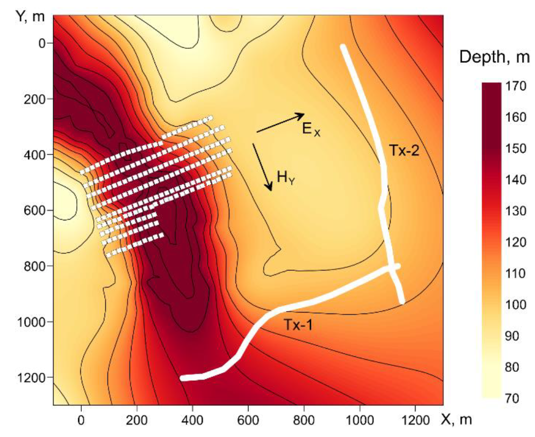
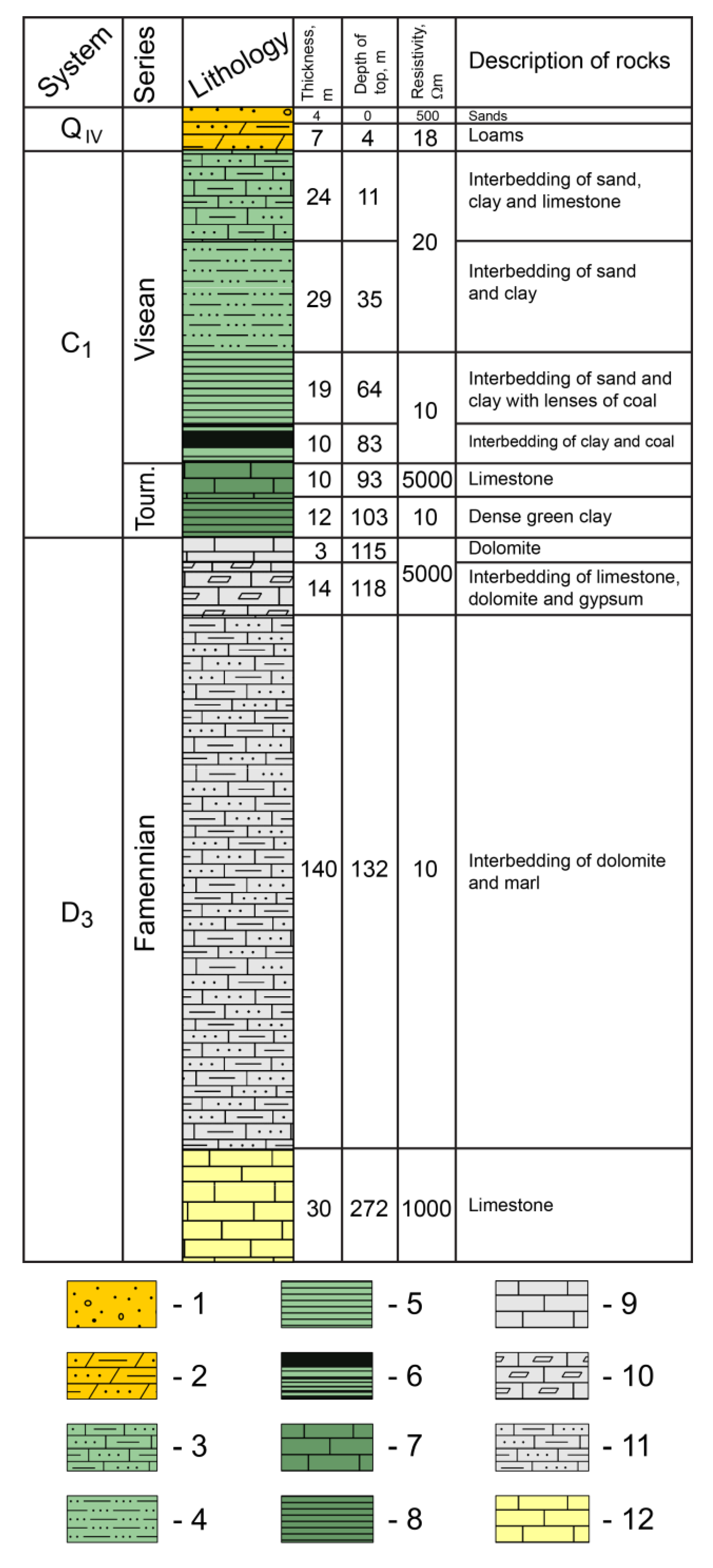
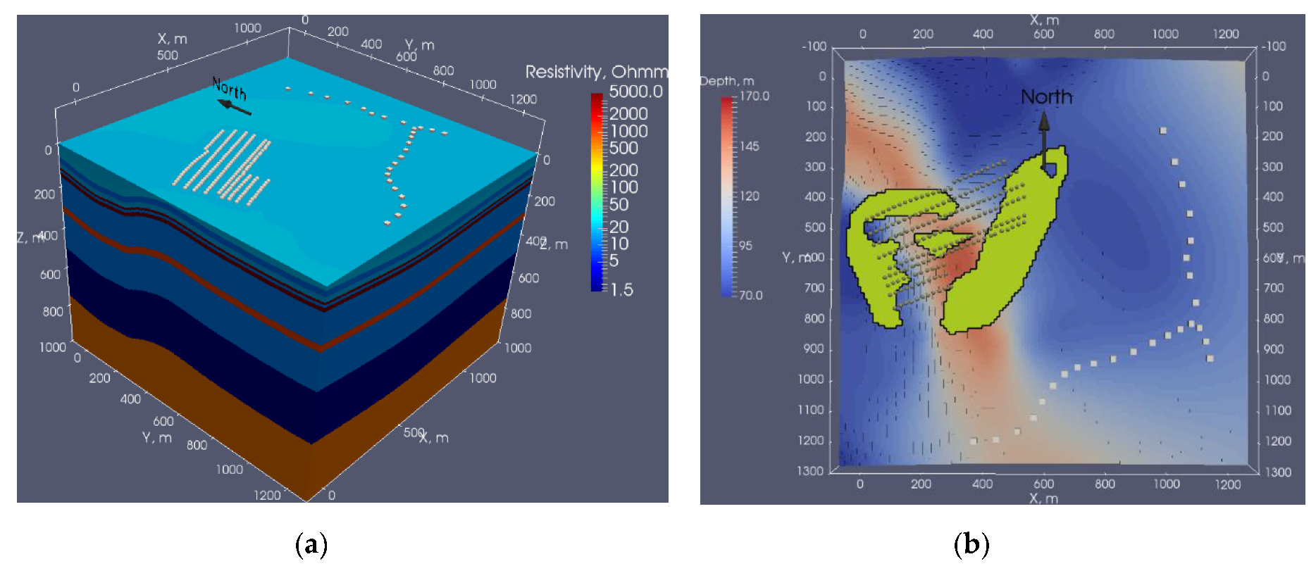
3.2. Conductivity Model of Aleksadrovka
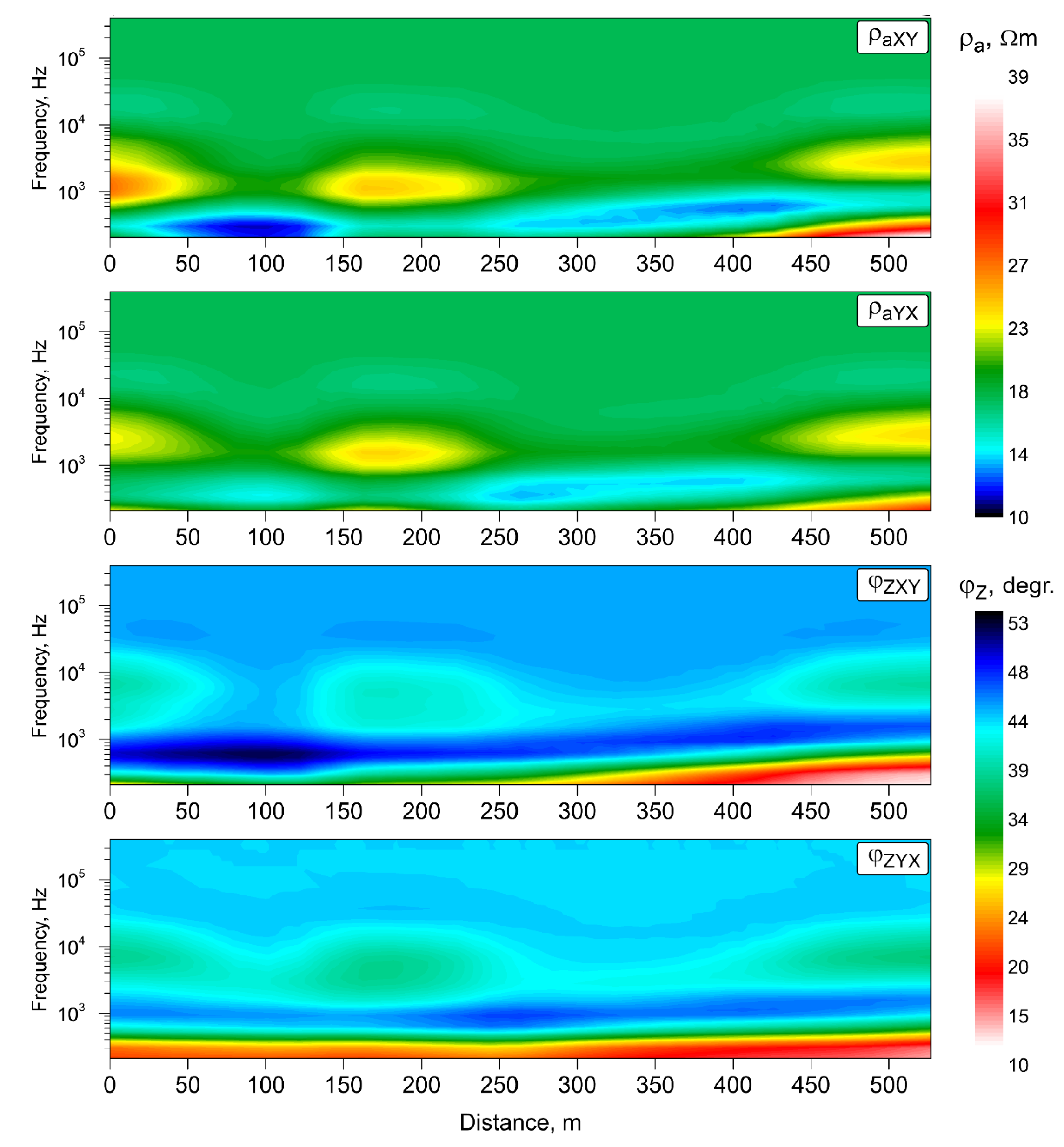
3.3. Numerical Simulation of Aleksadrovka
4. Discussion
Supplementary Materials
Author Contributions
Funding
Acknowledgments
Conflicts of Interest
Appendix A
References
- Hu, Y.-C.; Li, T.-L.; Fan, C.-S.; Wang, D.-Y.; Li, J.-P. Three-dimensional tensor controlled-source electromagnetic modeling based on the vector finite-element method. Appl. Geophys. 2015, 12, 35–46. [Google Scholar] [CrossRef]
- Li, X.; Pedersen, L.B. Controlled source tensor magnetotellurics. Geophysics 1991, 56, 1456–1462. [Google Scholar] [CrossRef]
- McMillan, M.S.; Oldenburg, D.W. Cooperative constrained inversion of multiple electromagnetic data sets. Geophysics 2014, 79, B173–B185. [Google Scholar] [CrossRef]
- Wang, T.; Wang, K.-P.; Tan, H.-D. Forward modeling and inversion of tensor CSAMT in 3D anisotropic media. Appl. Geophys. 2017, 14, 590–605. [Google Scholar] [CrossRef]
- Zonge, K.L.; Hughes, L.J. Controlled source audio-frequency magnetotellurics. In Electromagnetic Methods in Applied Geophysics; Applications, Series: Investigations in geophysics, No 3; SEG Library: Tulsa, OK, USA, 1991; Volume 2, pp. 713–809. [Google Scholar]
- Grayver, A.V.; Streich, R.; Ritter, O. Three-dimensional parallel distributed inversion of CSEM data using a direct forward solver. Geophys. J. Int. 2013, 193, 1432–1446. [Google Scholar] [CrossRef]
- Bastani, M. EnviroMT: A new Controlled Source/Radio Magnetotelluric System. Ph.D. Thesis, ACTA Universitatis Upsaliensis, Uppsala, Sweden, 2001; p. 179. [Google Scholar]
- Newman, G.A.; Recher, S.; Tezkan, B.; Neubauer, F.M. 3D inversion of a scalar radio magnetotelluric field data set. Geophysics 2003, 68, 791–802. [Google Scholar] [CrossRef]
- Saraev, A.; Simakov, A.; Shlykov, A.; Tezkan, B. Controlled-source radiomagnetotellurics: A tool for near surface investigations in remote regions. J. Appl. Geophys. 2017, 146, 228–237. [Google Scholar] [CrossRef]
- Tezkan, B. Radiomagnetotellurics, in Groundwater Geophysics—A Tool for Hydrogeology; Springer: Berlin/Heidelberg, Germany, 2008; pp. 295–317. [Google Scholar]
- Turberg, P.; Müller, I.; Flury, F. Hydrogeological investigation of porous environments by radio magnetotelluric-resistivity (RMT-R 12240 kHz). J. Appl. Geophys. 1994, 31, 133–143. [Google Scholar] [CrossRef]
- Spies, B.R.; Frischknecht, F.C. Electromagnetic Sounding. In Electromagnetic Methods in Applied Geophysics; Applications, Series: Investigations in geophysics, No 3; SEG Library: Tulsa, OK, USA, 1991; Volume 2. [Google Scholar]
- Shlykov, A.; Saraev, A. Estimating the Macroanisotropy of a Horizontally Layered Section from Controlled-Source Radiomagnetotelluric Soundings. Izv. Phys. Solid Earth 2015, 51, 583–601. [Google Scholar] [CrossRef]
- Kalscheuer, T.; Pedersen, L.B.; Siripunvaraporn, W. Radiomagnetotelluric two-dimensional forward and inverse modelling accounting for displacement currents. Geophys. J. Int. 2008, 175, 486–514. [Google Scholar] [CrossRef]
- Persson, L.; Pedersen, L.B. The importance of displacement currents in RMT measurements in high resistivity environments. J. Appl. Geophys. 2002, 51, 11–20. [Google Scholar] [CrossRef]
- Yavich, N.; Pushkarev, P.; Zhdanov, M. Application of a Finite-difference Solver with a Contraction Preconditioner to 3D EM Modeling in Mineral Exploration. In Proceedings of the Near Surface Geoscience 2016—First Conference on Geophysics for Mineral Exploration and Mining, EAGE, Barcelona, Spain, 4–8 September 2016. [Google Scholar]
- Cai, H.; Hu, X.; Li, J.; Endo, M.; Xiong, B. Parallelized 3D CSEM modeling using edge-based finite element with total field formulation and unstructured mesh. Comput. Geosci. 2017, 99, 125–134. [Google Scholar] [CrossRef]
- Grayver, A.V.; Bürg, M. Robust and scalable 3-D geo-electromagnetic modelling approach using the finite element method. Geophys. J. Int. 2014, 198, 110–125. [Google Scholar] [CrossRef]
- Streich, R. 3D finite-difference frequency-domain modeling of controlled-source electromagnetic data: Direct solution and optimization for high accuracy. Geophysics 2009, 74, F95–F105. [Google Scholar] [CrossRef]
- Mackie, R.L.; Smith, J.T.; Madden, T.R. Three-dimensional electromagnetic modeling using finite difference equations: The magnetotelluric example. Radio Sci. 1994, 29, 923–935. [Google Scholar] [CrossRef]
- Mulder, W.A. A robust solver for CSEM modelling on stretched grids. In Proceedings of the 69th EAGE Conference and Exhibition, London, UK, 11–14 June 2007. [Google Scholar]
- Yavich, N.; Scholl, C. Advances in multigrid solution of 3D forward MCSEM problem. In Proceedings of the 5th EAGE St. Petersburg International Conference and Exhibition on Geosciences, EAGE, Saint Petersburg, Russia, 2–5 April 2012. [Google Scholar]
- Yavich, N.; Zhdanov, M. Contraction pre-conditioner in finite-difference electromagnetic modelling. Geophys. J. Int. 2016, 206, 1718–1729. [Google Scholar] [CrossRef]
- Malovichko, M.; Tarasov, A.; Yavich, N.; Zhdanov, M. Mineral exploration with 3-D controlled-source electromagnetic method: A synthetic study of Sukhoi Log gold deposit. Geophys. J. Int. 2019, 219, 1698–1716. [Google Scholar] [CrossRef]
- Čuma, M.; Zhdanov, M.S.; Yoshioka, K. Parallel integral equation 3d (pie3d). In Proceedings of the Consortium for Electromagnetic Modeling and Inversion Annual Meeting, Salt Lake City, UT, USA, 22–27 March 2013. [Google Scholar]
- Monk, P.; Süli, E. A convergence analysis of Yee’s scheme on nonuniform grids. SIAM J. Numer. Anal. 1994, 31, 393–412. [Google Scholar] [CrossRef]
- Weiss, C.J.; Newman, G.A. Electromagnetic induction in a fully 3-D anisotropic earth. Geophysics 2002, 67, 1104–1114. [Google Scholar] [CrossRef]
- Zaslavsky, M.; Druskin, V.; Davydycheva, S.; Knizhnerman, L.; Abubakar, A.; Habashy, T. Hybrid finite-difference integral equation solver for 3D frequency domain anisotropic electromagnetic problems. Geophysics 2011, 76, F123–F137. [Google Scholar] [CrossRef]
- Van der Vorst, H.A. Bi-CGSTAB: A fast and smoothly converging variant of Bi-CG for the solution of nonsymmetric linear systems. SIAM J. Sci. Stat. Comput. 1992, 13, 631–644. [Google Scholar] [CrossRef]
- Zhdanov, M. Geophysical Electromagnetic Theory and Methods; Elsevier: Amsterdam, The Netherlands, 2009. [Google Scholar]
- Zhdanov, M. Foundations of Geophysical Electromagnetic Theory and Methods; Elsevier: Amsterdam, The Netherlands, 2018. [Google Scholar]
- Yavich, N.; Malovichko, M.; Khokhlov, N.; Zhdanov, M. Advanced Method of FD Electromagnetic Modeling Based on Contraction Operator. In Proceedings of the 79th EAGE Conference and Exhibition, Paris, France, 12–15 June 2017. [Google Scholar]
- Yoshika, K.; Zdanov, M.S. Electromagnetiv forward modeling based on the integral equation method using parallel computers. In Proceedings of the 75th Annual Inetrnational Meeting, Houston, TX, USA, 6–11 November 2005; pp. 550–553. [Google Scholar]
- Čuma, M.; Gribenko, A.; Zhdanov, M.S. Inversion of magnetotelluric data using integral equation approach with variable sensitivity domain: Application to EarthScope MT data. Phys. Earth Planet. Inter. 2017, 260, 113–127. [Google Scholar] [CrossRef]
- Modin, I.N.; Yakovleva, A.G. (Eds.) Electrical Exploration: A Guide to Electrical Exploration Practices for Students of Geophysical Specialties, 2nd ed.; PolisPRESS: Tver, Russia, 2018; Volume 1, p. 274. [Google Scholar]
- Zacharov, I.; Arslanov, R.; Gunin, M.; Stefonishin, D.; Bykov, A.; Pavlov, S.; Panarin, O.; Maliutin, A.; Rykovanov, S.; Fedorov, M. “Zhores”—Petaflops supercomputer for data-driven modeling, machine learning and artificial intelligence installed in Skolkovo Institute of Science and Technology. Open Eng. 2019, 9, 512–520. [Google Scholar] [CrossRef]


| # | Top, m | Thickness, m | Resistivity, Ωm |
|---|---|---|---|
| 1 | 108 | ||
| 2 | 0 | 8 | 500 |
| 3 | 8 | 92 | 20 |
| 4 | 100 | 10 | 104 |
| 5 | 110 | 10 | 20 |
| 6 | 120 | 104 |
| # | Top, m | Thickness, m | Resistivity, Ωm |
|---|---|---|---|
| 1 | 108 | ||
| 2 | 0 | 12 | 18 |
| 3 | 12 | 32 | 20 |
| 4 | 44 | 26 | 10 |
| 5 | 70 | 23 | 16 |
| 6 | 93 | 10 | 5000 |
| 7 | 103 | 12 | 11 |
| 8 | 115 | 17 | 5000 |
| 9 | 132 | 140 | 11 |
| 10 | 272 | 32 | 1000 |
| 11 | 304 | 176 | 11 |
| 12 | 480 | 250 | 1.5 |
| 13 | 730 | 670 |
| Grid Parameters | 192 Hz | 320 Hz | 576 Hz |
|---|---|---|---|
| FD grid dimensions | 114 × 110 × 151 | 136 × 128 × 183 | 166 × 158 × 138 |
| Num of discrete unknowns | 5.6 M | 9.4 M | 10.7 M |
| Grid step size in core domain, m | 7.4 | 5.7 | 4.3 |
| Core domain, m | 526 × 497 × 807 | 534 × 488 × 800 | 527 × 492 × 400 |
| Solver | Solver Step | 192 Hz | 320 Hz | 576 Hz |
|---|---|---|---|---|
| CO | RHS computation, sec | 2994 | 5762 | 9239 |
| Iteration count | 346 | 389 | 480 | |
| Iterative solver, sec | 3658 | 8177 | 13,673 | |
| Single iteration, sec | 10.6 | 21.0 | 28.5 | |
| GF | RHS computation, sec | 2993 | 5759 | 9258 |
| Iteration count | 3042 | 3713 | 5000 (*) | |
| Iterative solver, sec | 31,932 | 77,253 | 141,133 (*) | |
| Single iteration, sec | 10.5 | 20.8 | 28.2 |
| Frequency, Hz | Core Domain, m | Grid Step in Core Domain, m | Discrete Unknowns |
|---|---|---|---|
| 192 | 526 × 497 × 800 | 3.00 | 11.7 M |
| 320 | 534 × 488 × 800 | 3.00 | 16.2 M |
| 576 | 527 × 492 × 397 | 2.99 | 14.0 M |
| 960 | 524 × 497 × 300 | 3.00 | 10.9 M |
| 1500 | 525 × 493 × 200 | 2.99 | 11.0 M |
| 2500 | 530 × 489 × 150 | 3.00 | 13.5 M |
| 3500 | 531 × 490 × 150 | 3.00 | 17.1 M |
| 5500 | 529 × 490 × 147 | 2.73 | 25.2 M |
| 7500 | 529 × 491 × 148 | 2.34 | 34.5 M |
| 15,000 | 528 × 492 × 148 | 1.67 | 70.2 M |
| 25,000 | 528 × 493 × 150 | 1.95 | 47.5 M |
| 35,000 | 530 × 491 × 147 | 3.26 | 17.7 M |
| 55,000 | 528 × 491 × 97 | 2.56 | 23.4 M |
| 75,000 | 529 × 493 × 78 | 2.22 | 29.2 M |
| 150,000 | 530 × 492 × 38 | 1.54 | 45.9 M |
| 250,000 | 529 × 492 × 40 | 1.21 | 76.0 M |
| 350,000 | 528 × 493 × 19 | 1.00 | 86.9 M |
| 550,000 | 529 × 492 × 10 | 0.91 | 93.0 M |
| Frequency, Hz | Discrete Unknowns | RHS Computation, Sec | Iteration Count | Iterative Solver, Sec |
|---|---|---|---|---|
| 192 | 11.7 M | 398 | 459 | 732 |
| 320 | 16.2 M | 572 | 479 | 1076 |
| 576 | 14.0 M | 729 | 460 | 1043 |
| 960 | 10.9 M | 318 | 502 | 845 |
| 1500 | 11.0 M | 380 | 535 | 934 |
| 2500 | 13.5 M | 561 | 443 | 1052 |
| 3500 | 17.1 M | 765 | 447 | 1568 |
| 5500 | 25.2 M | 1208 | 665 | 3555 |
| 7500 | 34.5 M | 1795 | 553 | 4700 |
| 15,000 | 70.2 M | 4489 | 578 | 12,741 |
| 25,000 | 47.5 M | 3006 | 619 | 7264 |
| 35,000 | 17.7 M | 768 | 495 | 1766 |
| 55,000 | 23.4 M | 1122 | 436 | 2269 |
| 75,000 | 29.2 M | 1362 | 227 | 1947 |
| 150,000 | 45.9 M | 2304 | 64 | 956 |
| 250,000 | 76.0 M | 4140 | 21 | 855 |
| 350,000 | 86.9 M | 4120 | 17 | 1048 |
| 550,000 | 93.0 M | 3994 | 14 | 1108 |
© 2019 by the authors. Licensee MDPI, Basel, Switzerland. This article is an open access article distributed under the terms and conditions of the Creative Commons Attribution (CC BY) license (http://creativecommons.org/licenses/by/4.0/).
Share and Cite
Yavich, N.; Malovichko, M.; Shlykov, A. Parallel Simulation of Audio- and Radio-Magnetotelluric Data. Minerals 2020, 10, 42. https://doi.org/10.3390/min10010042
Yavich N, Malovichko M, Shlykov A. Parallel Simulation of Audio- and Radio-Magnetotelluric Data. Minerals. 2020; 10(1):42. https://doi.org/10.3390/min10010042
Chicago/Turabian StyleYavich, Nikolay, Mikhail Malovichko, and Arseny Shlykov. 2020. "Parallel Simulation of Audio- and Radio-Magnetotelluric Data" Minerals 10, no. 1: 42. https://doi.org/10.3390/min10010042
APA StyleYavich, N., Malovichko, M., & Shlykov, A. (2020). Parallel Simulation of Audio- and Radio-Magnetotelluric Data. Minerals, 10(1), 42. https://doi.org/10.3390/min10010042