Reference-Dependent Aggregation in Multi-AttributeGroup Decision-Making


Abstract
:1. Introduction
- (1)
- To investigate the impact of DMs psychological factors on the decision-making result, we propose for the first time two new operators based on RUs: the S-shaped and non-S-shaped operators. The DM can choose different RU operators to get the result according to his/her attitude toward the relative losses. To be specific, if the attitude of the DM is risk-seeking for relative losses, he/she can use the S-shaped operators (see Equation (11)) to select the optimal alternative. If the attitude of the DM is risk-averse for relative losses, he/she can apply the non-S-shaped operators (see, Equation (16)) in the decision-making process. If the attitude of a DM is risk-neutral, he/she can make decisions via the generalized ordered weighted multiple averaging (GOWMA) operator (see, Equation (18)) which is degenerated by the non-S-shaped operator. The main advantage of the RU operators is that they not only reflect the psychological character of the DM while the aforementioned aggregation methods fail to capture in the aggregation process, but also generate a family of aggregation operators by taking different parameters. Specifically, the RU operators can degenerate to the existing aggregation operators (see Table A1, Table A2 and Table A3 in Appendix A.3), which can be seen as the particular case of the RU operators.
- (2)
- To determine the associated weights for the multiple attributes and DMs, we propose an attribute- deviation weight model and a DMs-deviation weight model (see, models (19) and (20)). Going beyond the framework of existing weight models which ignored the dependence on the attribute variation (deviation), our new weight models consider the variations impacts of the attribute values on the determination of the weight in aggregation process. In addition, the attributes weights and the DMs weights are calculated by using attribute-deviation and DM-deviation models respectively, while the most research uses the same model to determine the associated weights for both attributes and DMs, sometimes leading to biased decision results.
- (3)
- We develop a new approach for MAGDM based on the RU operators and the weight models. In addition, the numerical examples are given to illustrate the application of the approach. Two novel findings emerge from the numerical analysis in Section 6. First, the optimal alternative will change to a relatively prudent alternative with the absolute risk aversion coefficient increasing. Second, the optimal alternative changes to a relatively risky one with the reference point (or, loss aversion coefficient) increasing.
2. Aggregation Operators for Risk-Seeking DMs Regarding Relative Losses
2.1. General Framework
- (1)
- v is strictly increasing;
- (2)
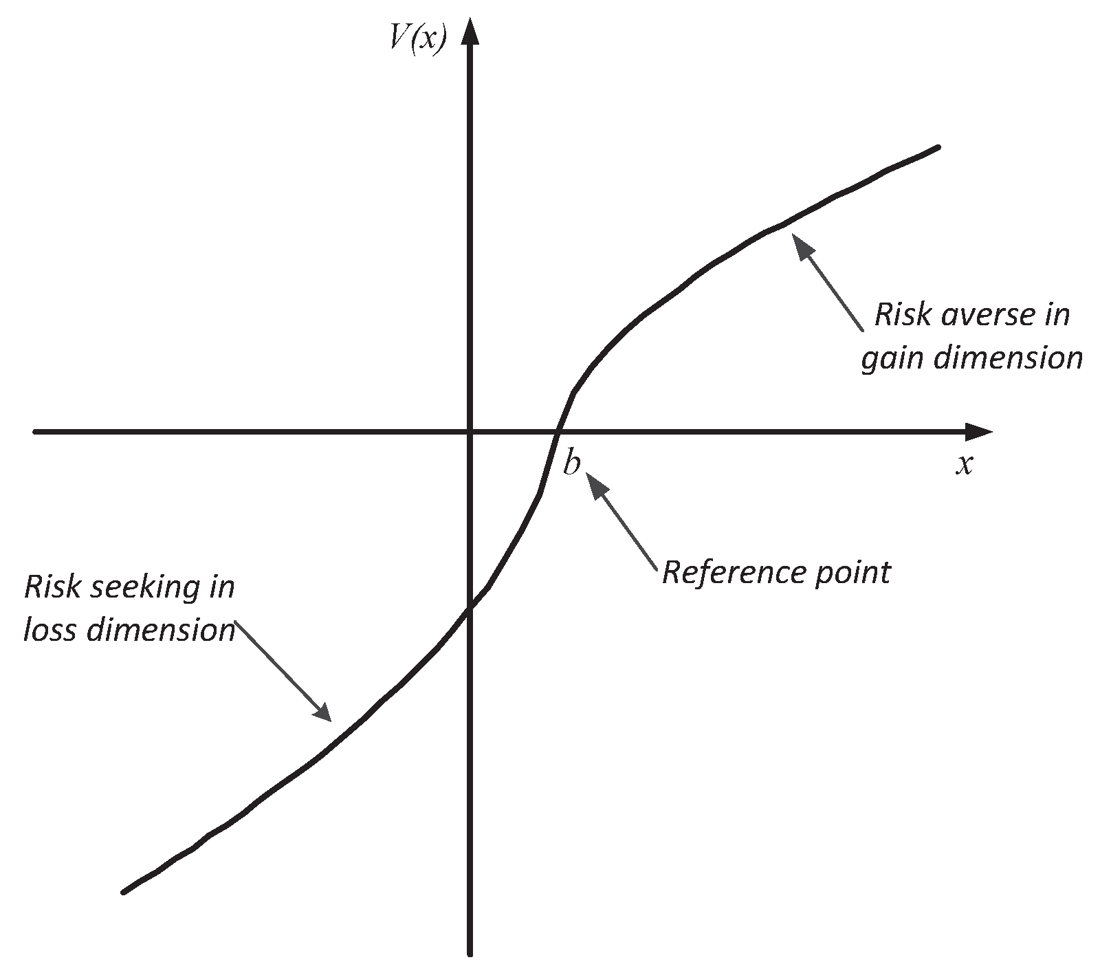
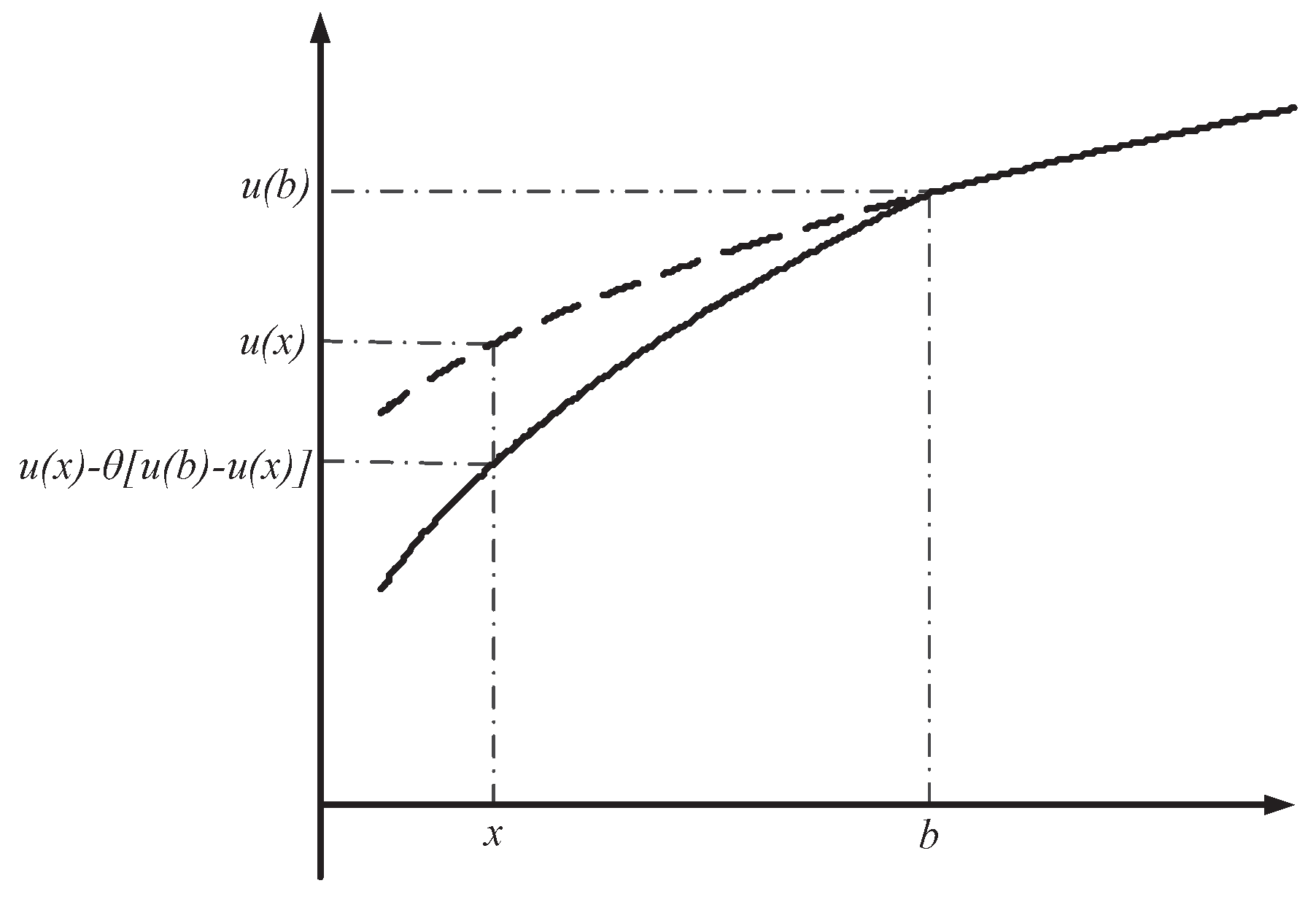
- v is convex for and concave for ;
- (3)
- v is asymmetry for : ;
- (4)
- for all , and .
- (1)
- (Monotonicity) For two vectors and with and the same reference points, then .
- (2)
- (Boundedness) If and , then .
- (3)
- (Commutativity) If is a permutation of , then .
- (4)
- (Idempotency) If for all , then .
2.2. Prospect Reference-Dependent Aggregation Operator
2.3. S-Shaped Hyperbolic Absolute Risk Aversion (HARA) Reference-Dependent Aggregation Operator
3. Aggregation Operators for Risk-Averse DMs Regarding Relative Losses
3.1. General Framework
3.2. Non-S-Shaped HARA Reference-Dependent Aggregation Operator
4. New Weight Models for Reference-Dependent Aggregation Operators
4.1. Weight Model for Attributes
- A weak ranking: ;
- A strict ranking: ;
- A ranking with multiples: ;
- An interval form: ;
- A ranking of differences: , for , , 0.
4.2. Weight Model for Decision Makers
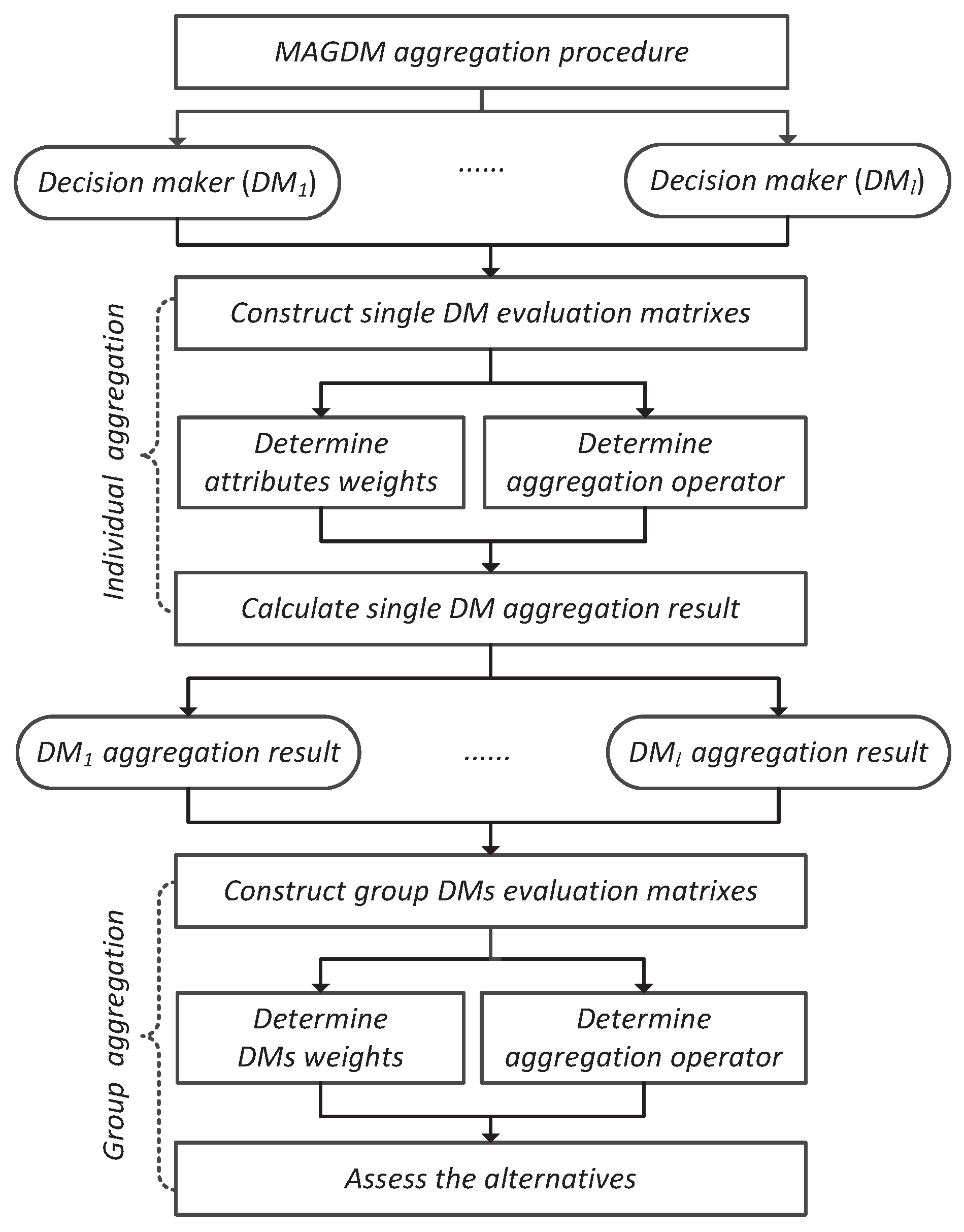
5. A New Reference-Dependent Aggregation Approach for MAGDM
- Step 1
- Transform the decision matrixes to the corresponding normalized version [8]:where is a set of profit attributes and is a set of cost attribute.
- Step 2
- Calculate the attribute weight vector of the decision matrix by solving the optimization problem in model (19) for .
- Step 3
- Step 4
- Calculate the DMs weights by solving the optimization problem in model (20).
- Step 5
- Aggregate all attribute values to obtain an overall preference value of the alternative by using the DM weight vector and the HOM operator given in Equation (17).
- Step 6
- Rank the collective overall preference values in the descending order and consequently, select the optimal alternative(s) (e.g., the one(s) with the greatest value ).
6. Numerical Examples
6.1. An Investment Selection Problem
- (1)
- The SHOMR operators (see, Equation (11)) and NHOMR operators (see, Equation (16)) can capture the psychological preference of the DM with regard to the input argument information, while the aggregation operators in Merigó & Casanovas [7] fail to consider in the decision-making process. Specifically, the above three cases clearly show that the optimal alternative highly depends on the reference point and the loss aversion coefficient θ; this confirms the significance of capturing psychological factors of DMs in the aggregation process. The DMs can choose different and θ based on their risk preference to select the optimal alternative.
- (2)
- The attribute-deviation weight model (see, model (19)) and DM-deviation weight model (see, model (20)) are constructed to determine the associated weights of the attributes and DMs, while the weights of the attributes and DMs are completely known in Merigó & Casanovas [7]. In fact, owing to the complexity and uncertainty of things in reality, the weights of the attributes and DMs are generally incomplete known.
- (3)
- The new aggregation operators can degenerate to the traditional aggregation operators including the OWGA operator [4], OWMA operator [8], CC-OWGA operator [32] and GOWMA operator [8], etc. (see, Table A1, Table A2 and Table A3 in Appendix A.3). In this way, the new aggregation approach can consider a wide range of scenarios according to the interests of the DM and select the alternative which is closest to his/her real interests.
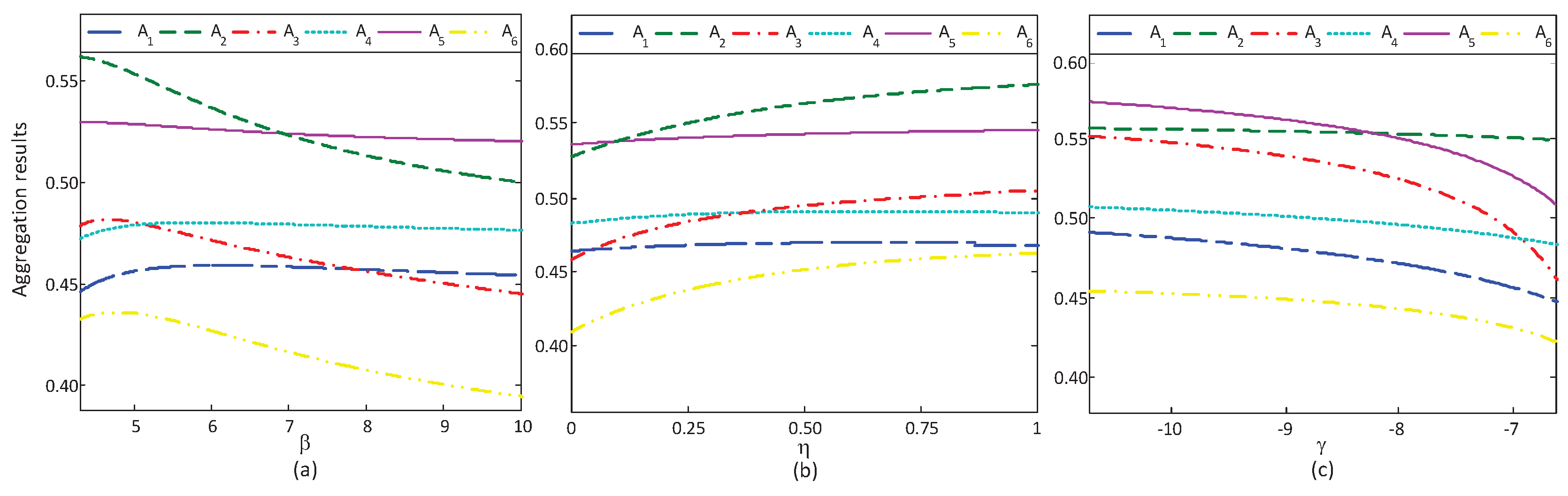
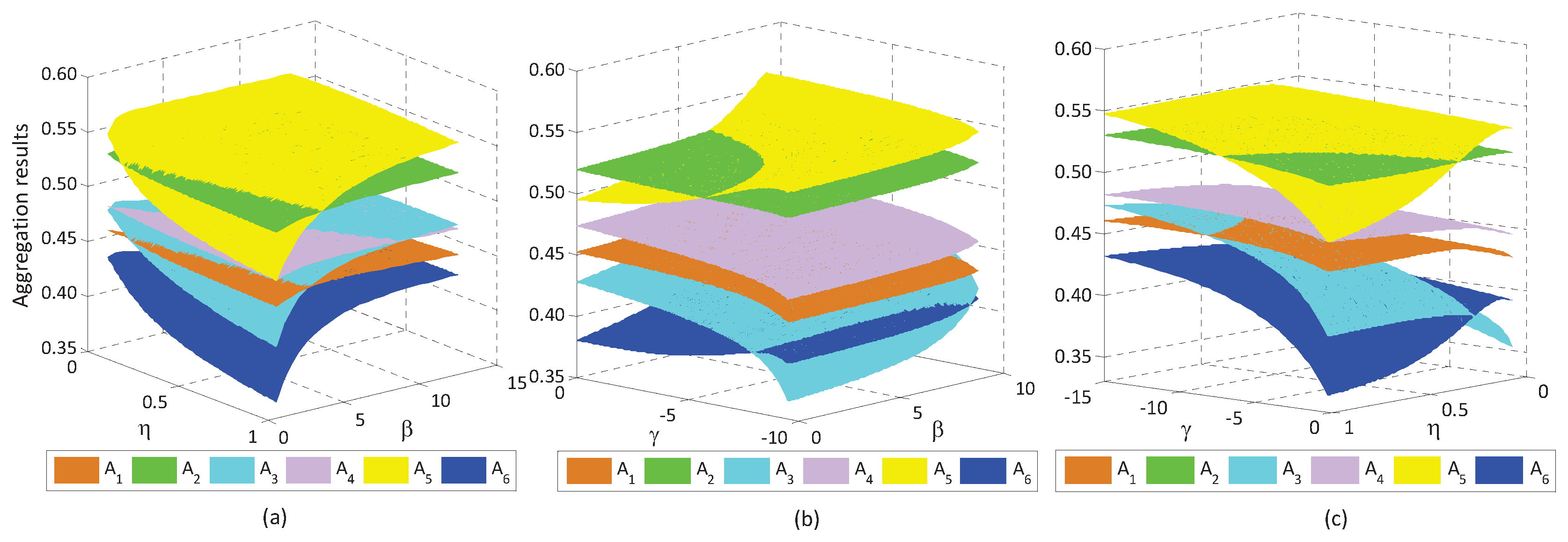
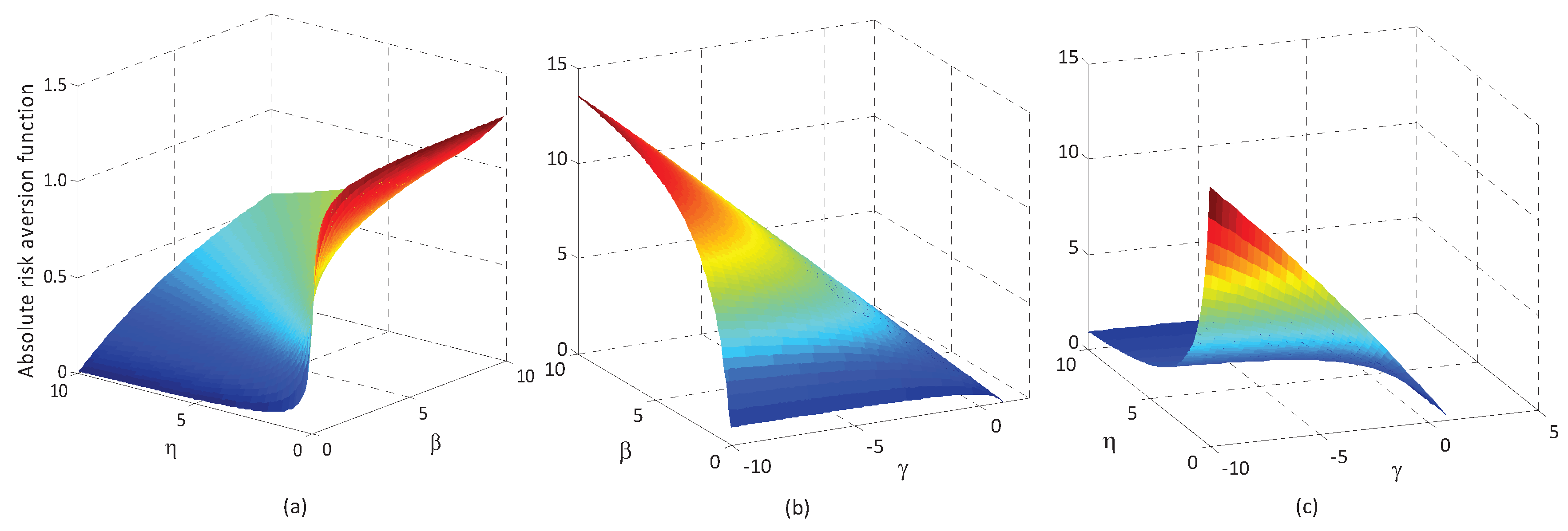
6.2. Sensitive Analysis of Reference-Dependent Aggregation Operators
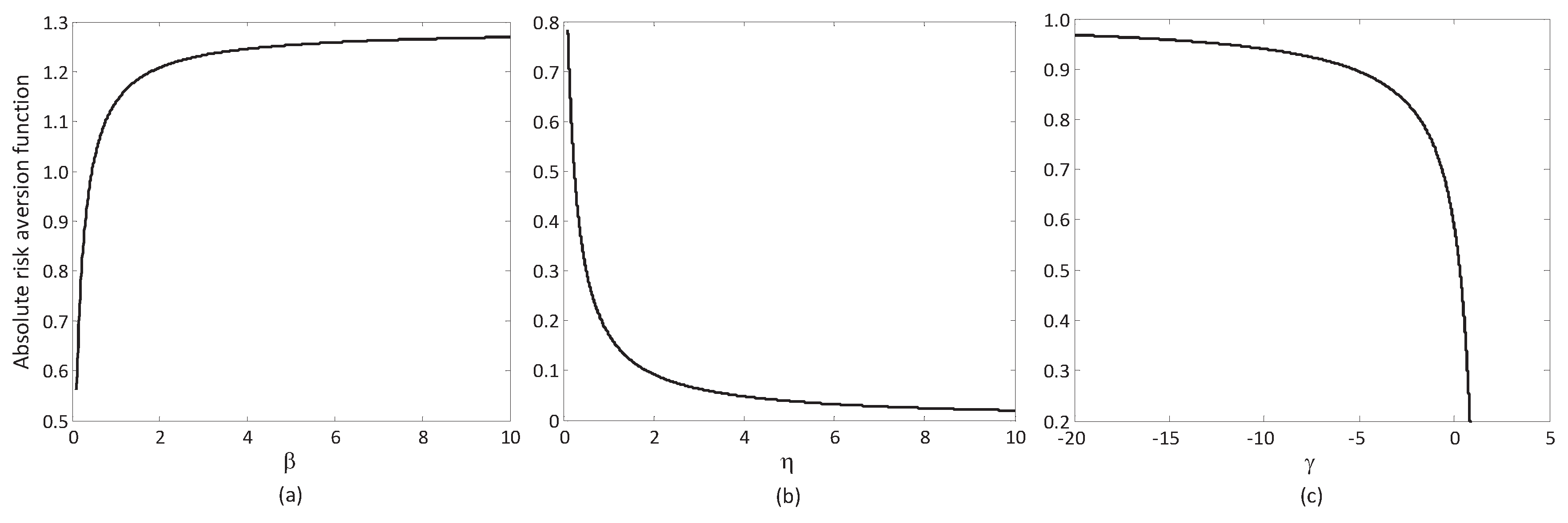
6.2.1. Sensitive Analysis of Parameters in the Basic Utility Function
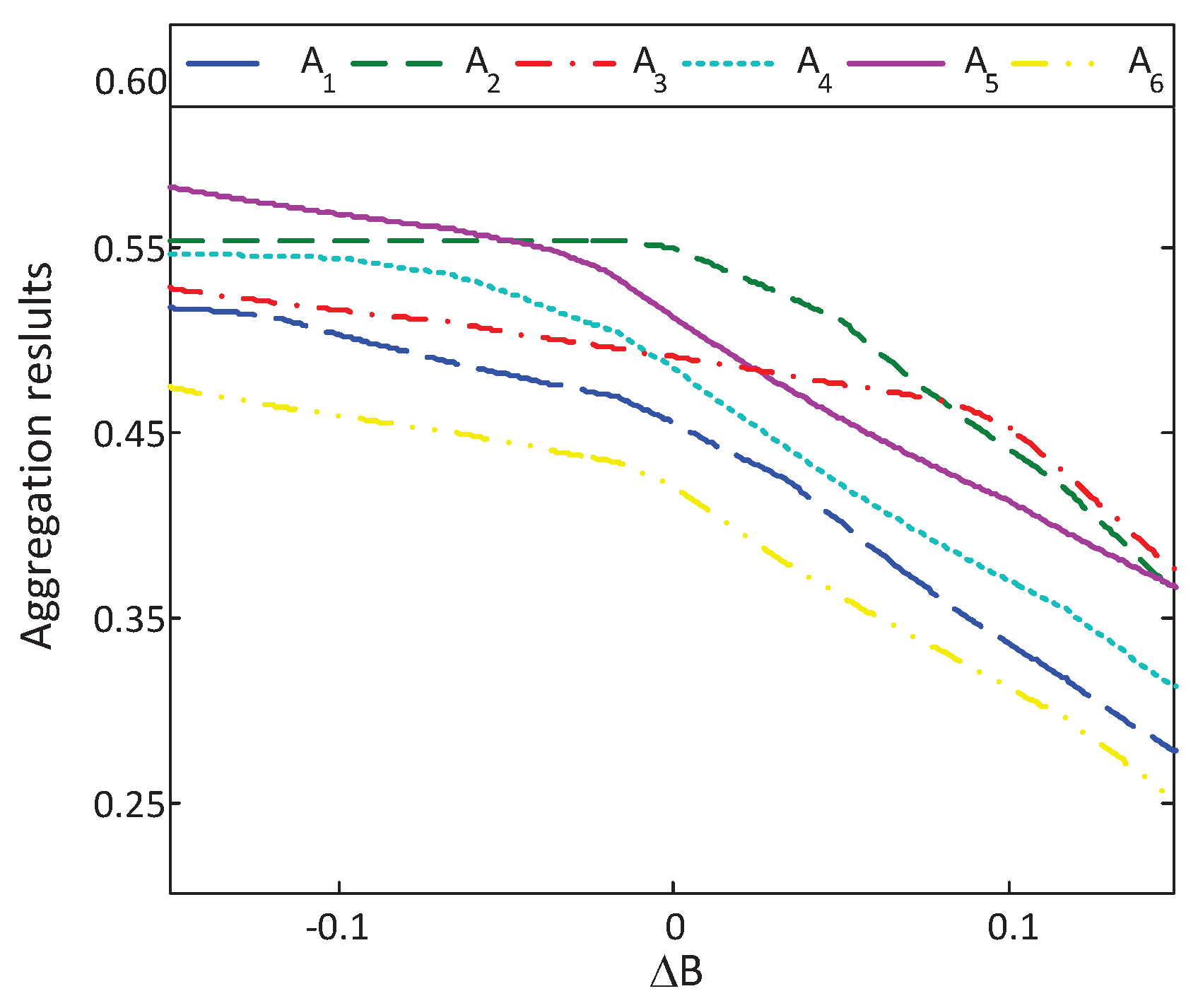
6.2.2. Sensitive Analysis of Reference Points
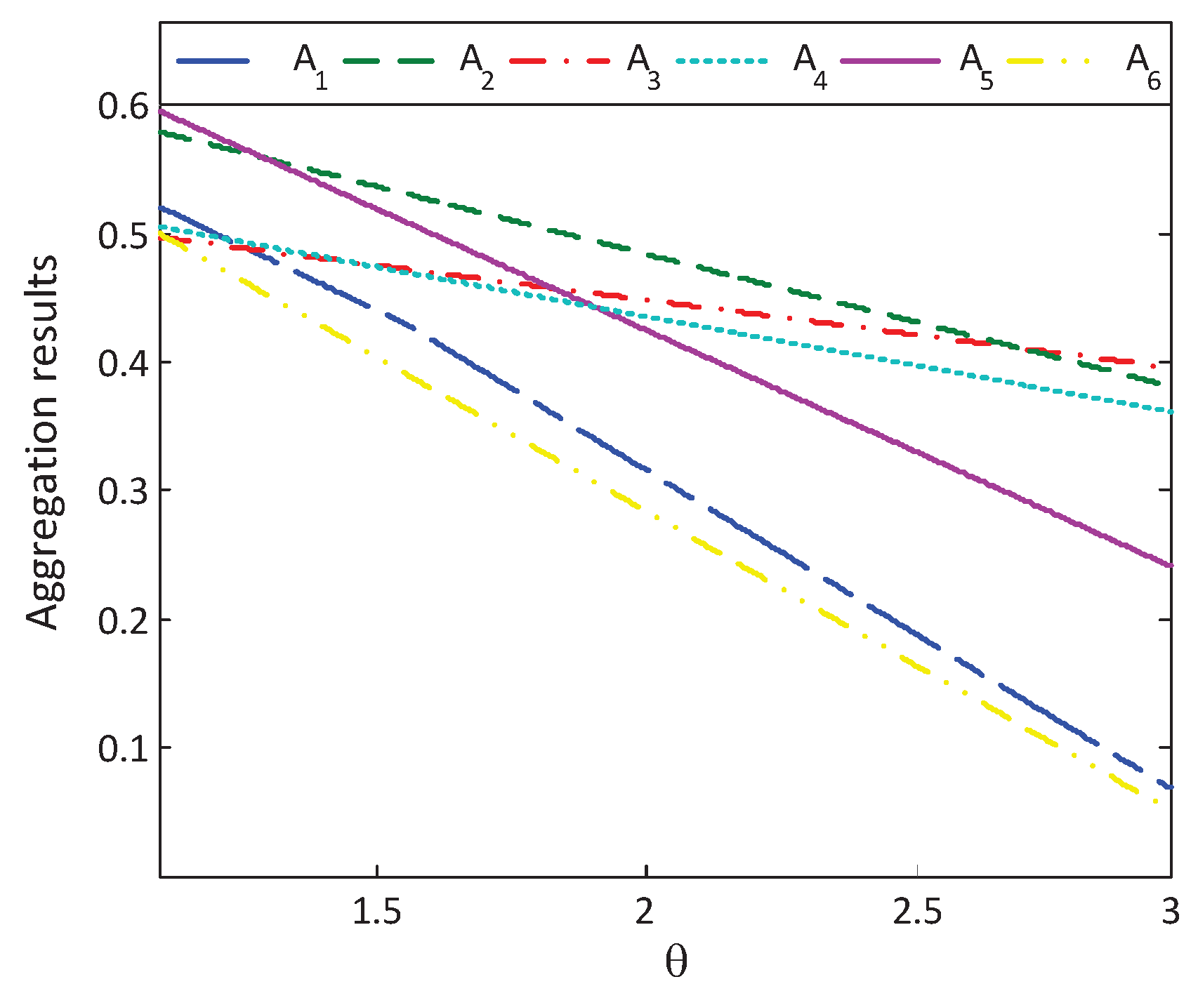
6.2.3. Sensitive Analysis of the Loss Aversion Coefficient
7. Conclusions
Acknowledgments
Author Contributions
Conflicts of Interest
Appendix A
Appendix A.1. Proof for Properties of SOMR Operator
- (1)
- (Monotonicity) For two vectors and with and the same reference points, then .
- (2)
- (Boundedness) If and , then .
- (3)
- (Commutativity) If is a permutation of , then .
- (4)
- (Idempotency) If for all , then .
- For , by taking the first-order condition of S with respect to , we have that,
- For , by taking the first-order condition of S with respect to , we have that,
Appendix A.2. Proof for Properties of NOMR Operator
- (1)
- (Monotonicity) For two vectors and with and the same reference points, then .
- (2)
- (Boundedness) If and , then . Especially, while .
- (3)
- (Commutativity) If is a permutation of , then .
- (4)
- (Idempotency). If for all , then .
- For , the first-order condition of N with respect to implies that,
- For , the first-order condition of N with respect to implies that,
Appendix A.3. Families of the Reference-Dependent Aggregation Operators

| λ | Formulation | The Name of Aggregation Operator | ||
|---|---|---|---|---|
| λ is odd and | Prospect gain ordered multiple reference-dependent operator (PGOMR) | |||
| Prospect gain ordered multiple operator (PGOM) | ||||
| Prospect loss ordered multiple reference-dependent operator (PLOMR) | ||||
| Prospect loss ordered multiple operator (PLOM) | ||||
| Ordered multiple reference-dependent operator (OMR) | ||||
| GOWMA operator [8] | ||||
| Prospect ordered multiple geometric reference-dependent operator (POMGR) | ||||
| Prospect ordered multiple geometric operator (POMG) | ||||
| Ordered multiple geometric reference-dependent aggregation operator (OMGR) | ||||
| Ordered multiple geometric aggregation operator (OMG) | ||||
| Constant prospect ordered multiple reference-dependent operator (CPOMR) | ||||
| Constant prospect ordered multiple dependent operator (CPOM) | ||||
| Constant ordered multiple reference-dependent operator (COMR) | ||||
| OWMA operator [8] | ||||
| Constant prospect ordered multiple geometric reference-dependent operator (CPOMGR) | ||||
| Constant prospect ordered multiple geometric operator (CPOMG) |
| λ | Formulation | The Name of Aggregation Operator | ||
|---|---|---|---|---|
| λ is odd and | S-shaped ordered multiple reference-dependent operator (SOMR) | |||
| S-shaped ordered multiple operator (SOM) | ||||
| Ordered multiple reference-dependent operator (OMR) | ||||
| GOWMA operator [8] | ||||
| S-shaped HARA ordered geometric reference-dependent operator (SHOGR) | ||||
| S-shaped HARA ordered geometric operator (SHOG) | ||||
| S-shaped ordered geometric reference-dependent operator (SOGR) | ||||
| S-shaped ordered geometric operator (SOG) | ||||
| Ordered multiple geometric reference-dependent operator (OMGR) | ||||
| Ordered multiple geometric operator (OMG) | ||||
| Constant HARA ordered multiple reference-dependent operator(CHOMR) | ||||
| Constant HARA ordered multiple operator (CHOM) | ||||
| Constant ordered multiple reference- dependent operator (COMR) | ||||
| Constant ordered multiple operator (COM) | ||||
| Constant ordered multiple reference-dependent operator (COMR) | ||||
| OWMA operator [8] |
| λ | θ | Formulation | The Name of Aggregation Operator | |
|---|---|---|---|---|
| , | Non-S-shaped ordered multiple reference-dependent basic operator (NOMRB) | |||
| GOWMA operator [8] | ||||
| Non-S-shaped HARA ordered reference-dependent geometric operator (NHORG) | ||||
| Ordered weighted utility geometric averaging-HARA operator (OWUGA-HARA) [32] | ||||
| Non-S-shaped ordered geometric operator (NOG) | ||||
| OWGA operator [4] | ||||
or | Constant non-S-shaped HARA ordered multiple reference-dependent operator (CNHOMR) | |||
| Constant HARA ordered multiple operator (CHOM) | ||||
| Constant non-S-shaped HARA orderedreference-dependent power operator(CNHORP) | ||||
| Constant ordered power operator (COP) | ||||
| Constant non-S-shaped ordered reference-dependent operator (CNOR) | ||||
| OWMA operator [8] | ||||
| Constant non-S-shaped HARA ordered geometric operator (CNHOG) | ||||
| CC-OWGA operator [32] | ||||
| Constant non-S-shaped ordered geometric operator (CNOG) | ||||
| OWGA operator [4] |
References
- Lu, J.; Zhang, G.Q.; Ruan, D.; Wu, F.J. Multi-Objective Group Decision Making: Methods, Software and Applications with Fuzzy Set Techniques; Imperial College Press: London, UK, 2007. [Google Scholar]
- Kahraman, C.; Onar, S.C.; Oztaysi, B. Fuzzy multicriteria decision-making: A literature review. Int. J. Comput. Intell. Syst. 2015, 8, 637–666. [Google Scholar] [CrossRef]
- Yager, R.R. On ordered weighted averaging aggregation operators in multicriteria decision making. IEEE Trans. Syst. Man Cybern. B 1988, 18, 183–190. [Google Scholar] [CrossRef]
- Xu, Z.S.; Da, Q.L. The ordered weighted geometric averaging operator. Int. J. Intell. Syst. 2002, 17, 709–716. [Google Scholar] [CrossRef]
- Yager, R.R.; Engemann, K.J.; Filev, D.P. On the concept of immediate probabilities. Int. J. Intell. Syst. 1995, 10, 373–397. [Google Scholar] [CrossRef]
- Merigó, J.M. Probabilities in the OWA operator. Expert Syst. Appl. 2012, 39, 11456–11467. [Google Scholar] [CrossRef]
- Merigó, J.M.; Casanovas, M. Decision-making with distance measures and induced aggregation operators. Comput. Ind. Eng. 2011, 60, 66–76. [Google Scholar] [CrossRef]
- Zhou, L.G.; Chen, H.Y.; Liu, J.P. Generalized multiple averaging operators and their applications to group decision making. Group Decis. Negot. 2013, 22, 331–358. [Google Scholar] [CrossRef]
- Dacey, R. The S-shaped utility function. Synthese 2003, 135, 243–272. [Google Scholar] [CrossRef]
- Kahneman, D.; Tversky, A. Prospect theory: An analysis of decision under risk. Econometrica 1979, 47, 263–291. [Google Scholar] [CrossRef]
- Shalev, J. Loss aversion equilibrium. Int. J. Game Theory 2000, 29, 269–287. [Google Scholar] [CrossRef]
- Meng, F.Y.; Tan, C.Q.; Chen, X.H. An approach to Atanassov’s interval-valued intuitionistic fuzzy multi-attribute decision making based on prospect theory. Int. J. Comput. Intell. Syst. 2015, 8, 591–605. [Google Scholar] [CrossRef]
- Zhang, H.Y.; Zhou, R.; Wang, J.Q.; Chen, X.H. An FMCDM approach to purchasing decision-making based on cloud model and prospect theory in e-commerce. Int. J. Comput. Intell. Syst. 2016, 9, 676–688. [Google Scholar] [CrossRef]
- Malul, M.; Rosenboim, M.; Shavit, T. So when are you loss averse? Testing the S-shaped function in pricing and allocation tasks. J. Econ. Psychol. 2013, 39, 101–112. [Google Scholar] [CrossRef]
- Driesen, B.; Perea, A.; Peters, H. On loss aversion in bimatrix games. Theory Decis. 2010, 68, 367–391. [Google Scholar] [CrossRef]
- Peters, H. A preference foundation for constant loss aversion. J. Math. Econ. 2012, 48, 21–25. [Google Scholar] [CrossRef]
- Abdellaoui, M.; Kemel, E. Eliciting prospect theory when consequences are measured in time units: Time is not money. Manag. Sci. 2014, 60, 1844–1859. [Google Scholar] [CrossRef]
- Shi, Y.; Cui, X.Y.; Yao, J.; Li, D. Dynamic trading with reference point adaptation and loss aversion. Oper. Res. 2015, 63, 789–806. [Google Scholar] [CrossRef]
- Fullér, R.; Majlender, P. On obtaining minimal variability OWA operator weights. Fuzzy Set. Syst. 2003, 136, 203–215. [Google Scholar] [CrossRef]
- Wang, Y.M.; Parkan, C. A preemptive goal programming method for aggregating OWA operator weights in group decision making. Inf. Sci. 2007, 177, 1867–1877. [Google Scholar] [CrossRef]
- Wang, Y.M.; Luo, Y.; Liu, X.W. Two new models for determining OWA operator weights. Comput. Ind. Eng. 2007, 52, 203–209. [Google Scholar] [CrossRef]
- Emrouznejad, A.; Amin, G.R. Improving minimax disparity model to determine the OWA operator weights. Inf. Sci. 2010, 180, 1477–1485. [Google Scholar] [CrossRef]
- Yari, G.; Chaji, A.R. Maximum Bayesian entropy method for determining ordered weighted averaging operator weights. Comput. Ind. Eng. 2012, 63, 338–342. [Google Scholar] [CrossRef]
- Ahn, B.S. Programming-based OWA operator weights with quadratic objective function. IEEE Trans. Fuzzy Syst. 2012, 20, 986–992. [Google Scholar] [CrossRef]
- Bustince, H.; Jurio, A.; Pradera, A.; Mesiar, R.; Beliakov, G. Generalization of the weighted voting method using penalty functions constructed via faithful restricted dissimilarity functions. Eur. J. Oper. Res. 2013, 225, 472–478. [Google Scholar] [CrossRef]
- Tohidi, G.; Khodadadi, M. The OWA weights of improved minimax disparity Model. Int. J. Intell. Syst. 2015, 30, 781–797. [Google Scholar] [CrossRef]
- Calvo, T.; Mayor, G.; Mesiar, R. Aggregation Operators: New Trends and Applications; Physica-Verlag: New York, NY, USA, 2002. [Google Scholar]
- Merton, R.C. Optimum consumption and portfolio rules in a continuous-time model. J. Econ. Theory 1971, 3, 373–413. [Google Scholar] [CrossRef]
- Grasselli, M. A stability result for the HARA class with stochastic interest rates. Insur. Math. Econ. 2003, 33, 611–627. [Google Scholar] [CrossRef]
- Jung, E.J.; Kim, J.H. Optimal investment strategies for the HARA utility under the constant elasticity of variance model. Insur. Math. Econ. 2012, 51, 667–673. [Google Scholar] [CrossRef]
- Cox, J.C.; Huang, C.F. Optimal consumption and portfolio policies when asset prices follow a diffusion process. J. Econ. Theory 1989, 49, 33–83. [Google Scholar] [CrossRef]
- Gao, J.W.; Li, M.; Liu, H.H. Generalized ordered weighted utility averaging-hyperbolic absolute risk aversion operators and their applications to group decision-making. Eur. J. Oper. Res. 2015, 243, 258–270. [Google Scholar] [CrossRef]
- Yager, R.R. Generalized OWA aggregation operators. Fuzzy Optim. Decis. Mak. 2004, 3, 93–107. [Google Scholar] [CrossRef]
- Aggarwal, M. Compensative weighted averaging aggregation operators. Appl. Soft Comput. 2015, 28, 368–378. [Google Scholar] [CrossRef]
- Ahn, B.S. Extreme point-based multi-attribute decision analysis with incomplete information. Eur. J. Oper. Res. 2015, 240, 748–755. [Google Scholar] [CrossRef]
- Kim, S.H.; Ahn, B.S. Interactive group decision making procedure under incomplete information. Eur. J. Oper. Res. 1999, 116, 498–507. [Google Scholar] [CrossRef]
- Guiso, L.; Paiella, M. Risk aversion, wealth, and background risk. J. Eur. Econ. Assoc. 2008, 6, 1109–1150. [Google Scholar] [CrossRef]


| Operator | z | |
|---|---|---|
| MR | ||
| PR | ||
| SR |
| Notations | Alternatives | Notations | Attributes |
|---|---|---|---|
| A chemical company | Benefits in the short term | ||
| A food company | Benefits in the mid-term | ||
| A computer company | Benefits in the long term | ||
| A car company | Risk of the investment | ||
| A furniture company | Difficulty of the investment | ||
| A pharmaceutical company | Other factors |
| 0.7 | 0.8 | 0.6 | 0.7 | 0.5 | 0.9 | 0.6 | 0.8 | 0.5 | 0.6 | 0.4 | 0.8 | 0.7 | 0.6 | 0.6 | 0.6 | 0.4 | 0.7 | |
| 0.8 | 0.6 | 0.9 | 0.7 | 0.6 | 0.7 | 0.7 | 0.6 | 0.8 | 0.6 | 0.7 | 0.7 | 0.7 | 0.6 | 0.7 | 0.6 | 0.6 | 0.7 | |
| 0.5 | 0.4 | 0.8 | 0.3 | 0.8 | 0.8 | 0.7 | 0.6 | 0.8 | 0.7 | 0.8 | 0.8 | 0.6 | 0.5 | 0.8 | 0.5 | 0.8 | 0.8 | |
| 0.6 | 0.7 | 0.6 | 0.7 | 0.8 | 0.6 | 0.6 | 0.7 | 0.5 | 0.6 | 0.8 | 0.7 | 0.6 | 0.7 | 0.7 | 0.5 | 0.8 | 0.6 | |
| 0.9 | 0.8 | 0.4 | 0.7 | 0.7 | 0.8 | 0.7 | 0.8 | 0.7 | 0.7 | 0.6 | 0.8 | 0.7 | 0.8 | 0.6 | 0.7 | 0.6 | 0.8 | |
| 0.8 | 0.3 | 0.7 | 0.7 | 0.6 | 0.7 | 0.6 | 0.4 | 0.8 | 0.7 | 0.6 | 0.7 | 0.4 | 0.5 | 0.9 | 0.7 | 0.6 | 0.6 | |
| β | η | γ | Overall Preference Value | Ordering | ||||||
|---|---|---|---|---|---|---|---|---|---|---|
| 1 | 12 | 0.5 | 0.0746 | 0.4502 | 0.5226 | 0.3793 | 0.4783 | 0.4539 | 0.3361 | |
| 3 | 5 | −3 | 0.5430 | 0.4557 | 0.5235 | 0.4110 | 0.4804 | 0.4709 | 0.3630 | |
| 4 | 2 | −5 | 1.6216 | 0.4598 | 0.5252 | 0.4395 | 0.4825 | 0.4907 | 0.3881 | |
| 5 | 0.5 | −7 | 5.3333 | 0.4613 | 0.5384 | 0.4854 | 0.4839 | 0.5336 | 0.4406 | |
| 6 | 0.45 | −6 | 5.7143 | 0.4597 | 0.5327 | 0.4815 | 0.4801 | 0.5329 | 0.4371 | |
| 7 | 0.3 | −9 | 8.8608 | 0.4578 | 0.5298 | 0.4795 | 0.4769 | 0.5307 | 0.4329 | |
| 9 | 0.1 | −11 | 14.400 | 0.4418 | 0.5241 | 0.4725 | 0.4711 | 0.5279 | 0.4290 | |
| 12 | 0.05 | −12 | 17.238 | 0.4388 | 0.5125 | 0.4688 | 0.4695 | 0.5210 | 0.4258 | |
© 2017 by the authors. Licensee MDPI, Basel, Switzerland. This article is an open access article distributed under the terms and conditions of the Creative Commons Attribution (CC BY) license ( http://creativecommons.org/licenses/by/4.0/).
Share and Cite
Gao, J.; Liu, H.
Reference-Dependent Aggregation in Multi-AttributeGroup Decision-Making
. Symmetry 2017, 9, 43.
https://doi.org/10.3390/sym9030043
Gao J, Liu H.
Reference-Dependent Aggregation in Multi-AttributeGroup Decision-Making
. Symmetry. 2017; 9(3):43.
https://doi.org/10.3390/sym9030043
Gao, Jianwei, and Huihui Liu.
2017. "Reference-Dependent Aggregation in Multi-AttributeGroup Decision-Making
" Symmetry 9, no. 3: 43.
https://doi.org/10.3390/sym9030043
Gao, J., & Liu, H.
(2017). Reference-Dependent Aggregation in Multi-AttributeGroup Decision-Making
. Symmetry, 9(3), 43.
https://doi.org/10.3390/sym9030043