Determinant Formulae of Matrices with Certain Symmetry and Its Applications

Abstract

In this paper, we introduce formulae for the determinants of matrices with certain symmetry. As applications, we will study the Alexander polynomial and the determinant of a periodic link which is presented as the closure of an oriented 4-tangle.

1. Introduction

A block matrix is a matrix which is partitioned into submatrices, called blocks, such that the subscripts of the blocks are defined in the same fashion as those for the elements of a matrix [1].

$$\left(\begin{array}{ccccc}{a}_{11}& a_{12}& a_{13}& a_{14}& a_{15}\\ a_{21}& a_{22}& a_{23}& a_{24}& a_{25}\\ a_{31}& a_{32}& a_{33}& a_{34}& a_{35}\\ a_{41}& a_{42}& a_{43}& a_{44}& a_{45}\\ a_{51}& a_{52}& a_{11}& a_{54}& a_{55}\end{array}\right)=\left(\begin{array}{cc}{A}_{11}& A_{12}\\ A_{21}& A_{22}\end{array}\right).$$

Let us consider periodic subject that consists of finite number of units with the same properties, see Figure 1. There are 5 subjects with the same properties which are arranged periodically. The brown color is used to depict their periodical placement, while the green color in the second and third figure presents an extra relationship which is acting between neighbouring two subjects.

Figure 1. Type of periodic subject.

The matrix encoding the properties of the whole subject can be presented by block matrices. In the first picture in Figure 1, there are a finite number of units which are placed periodically but there are no interaction between units as seen. The matrix for the periodic subject will be of the form

$$\left(\begin{array}{cccc}A& O& \cdots & O\\ O& A& \cdots & O\\ ⋮& ⋮& \ddots & ⋮\\ O& O& \dots & A\end{array}\right).$$

(1)

Indeed, the determinant of the matrix is ${(detA)}^n$.

In the second picture in Figure 1, there are a finite number of units which are placed periodically and each unit is affected by neighbouring units as seen. The matrix for such a periodic subject is of the form

$$\left(\begin{array}{ccccc}A& O& \cdots & O& B\\ O& A& \cdots & O& B\\ ⋮& ⋮& \ddots & ⋮& ⋮\\ O& O& \cdots & A& B\\ C& C& \cdots & C& nD\end{array}\right).$$

(2)

In [2], the authors showed that the determinant of such a matrix is given by $n^r{(det\left(A\right))}^{n-1}det\left(\begin{array}{cc}A& B\\ C& D\end{array}\right)$, where D is an $r\times r$ matrix.

On the other hand, in the last picture in Figure 1, there are a finite number of units which are placed periodically and each unit is affected by the periodic structure itself (rather than neighbouring units). The matrix for such a periodic object can be presented by a matrix of the form

$$\left(\begin{array}{ccccccccc}A& O& O& \cdots & O& -B& -B& \cdots & -B\\ O& A& O& \cdots & O& B& O& \cdots & O\\ O& O& A& \cdots & O& O& B& \cdots & O\\ ⋮& ⋮& ⋮& \ddots & ⋮& ⋮& ⋮& \ddots & ⋮\\ O& O& O& \cdots & A& O& O& \cdots & B\\ -C& C& O& \cdots & O& 2D& D& \cdots & D\\ -C& O& C& \cdots & O& D& 2D& \cdots & D\\ ⋮& ⋮& ⋮& \ddots & ⋮& ⋮& ⋮& \ddots & ⋮\\ -C& O& O& \cdots & C& D& D& \cdots & 2D\end{array}\right)$$

(3)

or a matrix of the form

$$\left(\begin{array}{ccccccccc}A& O& O& \cdots & O& -B& -B& \cdots & -B\\ O& A& O& \cdots & O& B& O& \cdots & O\\ O& O& A& \cdots & O& O& B& \cdots & O\\ ⋮& ⋮& ⋮& \ddots & ⋮& ⋮& ⋮& \ddots & ⋮\\ O& O& O& \cdots & A& O& O& \cdots & B\\ -C& C& O& \cdots & O& D+E& D& \cdots & D\\ -C& O& C& \cdots & O& E& D+E& \cdots & D\\ ⋮& ⋮& ⋮& \ddots & ⋮& ⋮& ⋮& \ddots & ⋮\\ -C& O& O& \cdots & C& E& E& \cdots & D+E\end{array}\right).$$

(4)

The applications in the last section will be helpful to understand the difference between (3) and (4).

In this paper, we will show that the determinant of the matrix (3) is

$$n^{r}det\left(A\right){\left\{det\left(\begin{array}{cc}A& B\\ C& D\end{array}\right)\right\}}^{n-1},$$

while the determinant of the matrix (4) is

$$det\left(A\right)\sum _{k=1}^n{\left\{det\left(\begin{array}{cc}A& B\\ C& D\end{array}\right)\right\}}^{n-k}{\left\{det\left(\begin{array}{cc}A& B\\ C& E\end{array}\right)\right\}}^{k-1}.$$

As an application, we will find the Alexander polynomial and the determinant of a periodic link (Theorems 4–7). Notice that, if a matrix M is singular, then we define ${(det\left(M\right))}^0=1$.

2. Determinants

In this section, we introduce formulae for the determinants of block matrices (3) and (4).

Theorem 1.

Let $A,B,C,$ and D be matrices of size $m\times m,m\times r,r\times m$ and $r\times r$, respectively and O the zero-matrix. Then

$$det\left(\begin{array}{ccccccccc}A& O& O& \cdots & O& -B& -B& \cdots & -B\\ O& A& O& \cdots & O& B& O& \cdots & O\\ O& O& A& \cdots & O& O& B& \cdots & O\\ ⋮& ⋮& ⋮& \ddots & ⋮& ⋮& ⋮& \ddots & ⋮\\ O& O& O& \cdots & A& O& O& \cdots & B\\ -C& C& O& \cdots & O& 2D& D& \cdots & D\\ -C& O& C& \cdots & O& D& 2D& \cdots & D\\ ⋮& ⋮& ⋮& \ddots & ⋮& ⋮& ⋮& \ddots & ⋮\\ -C& O& O& \cdots & C& D& D& \cdots & 2D\end{array}\right)=n^{r}det\left(A\right){\left\{det\left(\begin{array}{cc}A& B\\ C& D\end{array}\right)\right\}}^{n-1},$$

where the number of A’s in the diagonal is n and the number of $\left(2D\right)$’s in the diagonal is $n-1$ $(n\ge 2)$.

Proof. 

The identity can be obtained by elementary determinant calculation. We put the detailed proof at Appendix A for the convenience of readers. ☐

Theorem 2.

Let $A,B,C,D$ and E be matrices of size $m\times m,m\times 1,1\times m,1\times 1$ and $1\times 1$, respectively and O the zero-matrix. Then

$$det\left(\begin{array}{ccccccccc}A& O& O& \cdots & O& -B& -B& \cdots & -B\\ O& A& O& \cdots & O& B& O& \cdots & O\\ O& O& A& \cdots & O& O& B& \cdots & O\\ ⋮& ⋮& ⋮& \ddots & ⋮& ⋮& ⋮& \ddots & ⋮\\ O& O& O& \cdots & A& O& O& \cdots & B\\ -C& C& O& \cdots & O& D+E& D& \cdots & D\\ -C& O& C& \cdots & O& E& D+E& \cdots & D\\ ⋮& ⋮& ⋮& \ddots & ⋮& ⋮& ⋮& \ddots & ⋮\\ -C& O& O& \cdots & C& E& E& \cdots & D+E\end{array}\right)$$

$$=det\left(A\right)\sum _{k=1}^n{\left\{det\left(\begin{array}{cc}A& B\\ C& D\end{array}\right)\right\}}^{n-k}{\left\{det\left(\begin{array}{cc}A& B\\ C& E\end{array}\right)\right\}}^{k-1},$$

where the number of A’s in the diagonal is n and the number of $D+E$’s in the diagonal is $n-1(n\ge 2)$.

Proof. 

$$\begin{array}{ccc}\hfill LHS& \begin{array}{c}=\\ \left(1\right)\end{array}& det\left(\begin{array}{|ccccccccc|}\hline A& O& O& \cdots & O& -B& -B& \cdots & -B\\ O& A& O& \cdots & O& 2B& B& \cdots & B\\ O& O& A& \cdots & O& B& 2B& \cdots & B\\ ⋮& ⋮& ⋮& \ddots & ⋮& ⋮& ⋮& \ddots & ⋮\\ O& O& O& \cdots & A& B& B& \cdots & 2B\\ O& C& O& \cdots & O& D+E& D& \cdots & D\\ O& O& C& \cdots & O& E& D+E& \cdots & D\\ ⋮& ⋮& ⋮& \ddots & ⋮& ⋮& ⋮& \ddots & ⋮\\ O& O& O& \cdots & C& E& E& \cdots & D+E\\ \hline\end{array}\right)\hfill \\ & \begin{array}{c}=\\ \left(2\right)\end{array}& det\left(A\right){\displaystyle \sum _{k=1}^n}{\left\{det\left(\begin{array}{cc}A& B\\ C& D\end{array}\right)\right\}}^{n-k}{\left\{det\left(\begin{array}{cc}A& B\\ C& E\end{array}\right)\right\}}^{k-1}.\hfill \end{array}$$

The identity can be obtained by elementary determinant calculation. The identity $\left(1\right)$ comes by adding the kth column to the first column and then, adding the $(-1)$(the first row) to the kth row for any $k=2,3,\cdots ,n$, while the identity $\left(2\right)$ can be found in Appendix A. ☐

Remark 1.

If A is invertible, then Theorems 1 and 2 can be proved by using the Schur complement. We put those proofs at Appendix B. The Authors appreciate such valuable comments given by our reviewer.

3. Application: Alexander Polynomials and the Determinants of Periodic Links

We start this section by reviewing results of knot theory which are related with the calculation of the Alexander polynomial and the determinant of a link, see [2,3,4] in detail.

A knot K is an embedding $K:S^1\hookrightarrow {\mathbb{R}}^3$ of $S^1$ into the 3-space ${\mathbb{R}}^3$. A link is a finite disjoint union of knots: $L=K_1\cup \cdots \cup K_n$. Each knot $K_i$ is called a component of the link L. Two links L and $L^{\prime }$ are equivalent (or ambient isotopic) if one can be transformed into the other via a deformation of ${\mathbb{R}}^3$ upon itself. 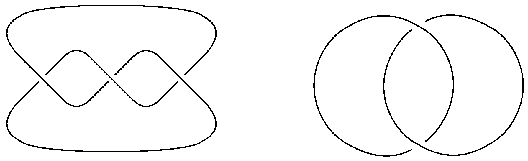A diagram of a link L is a regular projection image $p\left(L\right)$ from the link L into ${\mathbb{R}}^2$ such that the over-path and the under-path at each double points of $p\left(L\right)$ are distinguished. 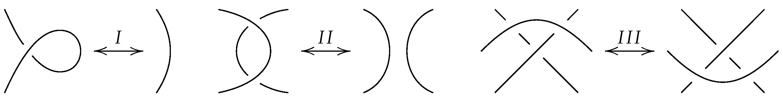There are examples of a knot and a link in Figure 2. Two link diagrams are equivalent if one can be transformed into another by a finite sequence of Reidemeister moves in Figure 3.

Figure 2. A trefoil knot diagram and a Hopf link diagram.

Figure 3. Reidemeister moves.

A Seifert surface for an oriented link L in $S^3$ is a connected compact oriented surface contained in $S^3$ which has L as its boundary. The following Seifert algorithm is one way to get a Seifert surface from a diagram D of L.

Let D be a diagram of an oriented link L. In a small neighborhood of each crossing, make the following local change to the diagram;

• Delete the crossing and reconnect the loose ends in the only way compatible with the orientation.

When this has been done at every crossing, the diagram becomes a set of disjoint simple loops in the plane. It is a diagram with no crossings. These loops are called Seifert circles. By attaching a disc to each Seifert circle and by connecting a half-twisted band at the place of each crossing of D according to the crossing sign, we get a Seifert surface F for L.

The Seifert graph $\mathsf{\Gamma }$ of F is constructed as follows;

• Associate a vertex with each Seifert circle and connect two vertices with an edge if their Seifert circles are connected by a twisted band.

Note that the Seifert graph $\mathsf{\Gamma }$ is planar, and that if D is connected, so does $\mathsf{\Gamma }$. Since $\mathsf{\Gamma }$ is a deformation retract of a Seifert surface F, their homology groups are isomorphic: $H_1\left(F\right)\cong H_1\left(\mathsf{\Gamma }\right)$. Let T be a spanning tree for $\mathsf{\Gamma }$. For each edge $e\in E\left(\mathsf{\Gamma }\right)\backslash E\left(T\right)$, $T\cup \left\{e\right\}$ contains the unique simple closed circuit $T_e$ which represents an 1-cycle in $H_1\left(F\right)$. The set $\{T_e|e\in E\left(\mathsf{\Gamma }\right)\backslash E\left(T\right)\}$ of these 1-cycles is a homology basis for F. For such a circuit $T_e$, let $T_e^{+}$ denote the circuit in $S^3$ obtained by lifting slightly along the positive normal direction of F. For $E\left(\mathsf{\Gamma }\right)\backslash E\left(T\right)=\{e_1,\cdots ,e_n\}$, the linking number between $T_{e_i}$ and $T_{e_j}^{+}$ is defined by

$$lk(T_{e_i},T_{e_j}^{+})=\frac{1}{2}\sum _{\mathrm{crossing}c\in T_{e_i}\cap T_{e_j}^{+}}sign\left(c\right).$$

A Seifert matrix of L associated to F is the $n\times n$ matrix $M=\left(m_{ij}\right)$ defined by

$$m_{ij}=lk(T_{e_i},T_{e_j}^{+}),$$

where $E\left(\mathsf{\Gamma }\right)\backslash E\left(T\right)=\{e_1,\cdots ,e_n\}$. A Seifert matrix of L depends on the Seifert surface F and the choice of generators of $H_1\left(F\right)$.

Let M be any Seifert matrix for an oriented link L. The Alexander polynomial ${\mathsf{\Delta }}_L\left(t\right)\in \mathbb{Z}[t,t^{-1}]$ and determinant of L are defined by

$$\begin{array}{ccc}\hfill {\mathsf{\Delta }}_L\left(t\right)& \doteq & det(t^{\frac{1}{2}}M-t^{-\frac{1}{2}}{M}^T)\hfill \\ \hfill det\left(L\right)& =& |det(M+M^T)|\hfill \end{array}$$

For details, see [4,5].

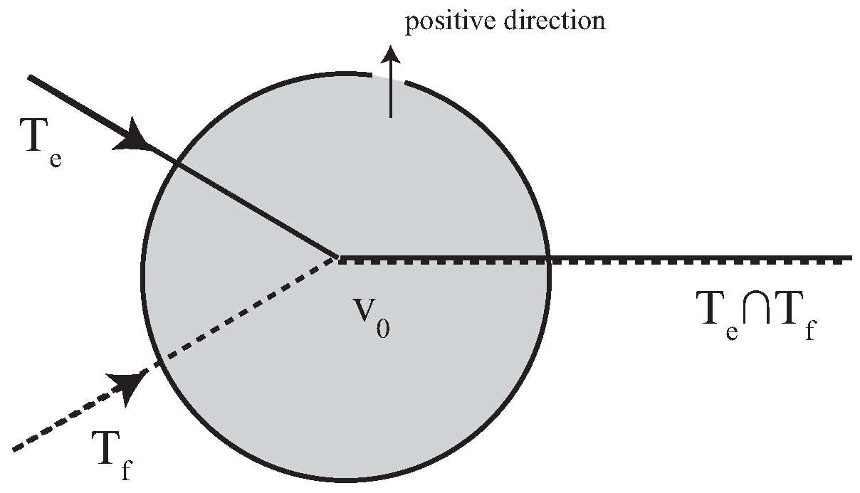
For $e,f\in E\left(\mathsf{\Gamma }\right)\backslash E\left(T\right)$, $T_e\cap T_f$ is either an empty set, one vertex or a simple path in the spanning tree T. If $T_e\cap T_f$ is a simple path, $v_0$ and $v_1$ are two ends of $T_e\cap T_f$, we may assume that the neighborhood of $v_0$ looks like Figure 4. In other words, the cyclic order of edges incident to $v_0$ is given by $T_e\cap T_f,T_e,T_f$ with respect to the positive normal direction of the Seifert surface. Also we may assume that the directions of $T_e$ and $T_f$ are given so that $v_0$ is the starting point of $T_e\cap T_f$. For, if the direction is reversed, one can change the direction to adapt to our setting so that the resulting linking number changes its sign.

Figure 4. $T_e\cap T_f$.

In [6], the authors showed the following proposition which is the key tool to calculate the linking numbers for Seifert matrix of a link.

The Alexander polynomial of a knot or a link is the first polynomial of the knot theory [7]. The polynomial was reformulate and derived in several different ways over the next 50 years. Perhaps the most satisfying of these is from the homology of the branched cyclic covering space of the knot complement. This reveals the underlying geometry and generalizes to higher dimensions and to a multi-variable version for links. See [4]. Many researchers reformulate the Alexander polynomial as a state sum, Kauffman [8] and Conway [9], etc. Recently, many authors interested in the twisted Alexander polynomial and Knot Floer homology, it provides geometric information of a knot or a link, see [10,11,12,13]. The Alexander polynomial is categorified by Knot Floer homology, see [14,15]. Furthermore, since Alexander polynomial is a topological content of quantum invariants, Alexander polynomial is one of the most important invarinat of knot theory, see [16].

Proposition 1

([6]). For $e,f\in E\left(\mathsf{\Gamma }\right)\backslash E\left(T\right)$, let p and q denote the numbers of edges in $T_e\cap T_f$ corresponding to positive crossings and negative crossings, respectively. Suppose that the local shape of $T_e\cap T_f$ in F looks like Figure 4. Then,

$$lk(T_e,T_f^{+})=\left\{\begin{array}{cc}-\frac{1}{2}(p-q),\hfill & \mathit{if}p+q\mathit{is}\mathit{even};\hfill \\ -\frac{1}{2}(p-q+1),\hfill & \mathit{if}p+q\mathit{is}\mathit{odd},\mathrm{and}\hfill \end{array}\right.$$

$$lk(T_f,T_e^{+})=\left\{\begin{array}{cc}-\frac{1}{2}(p-q),\hfill & \mathit{if}p+q\mathit{is}\mathit{even};\hfill \\ -\frac{1}{2}(p-q-1),\hfill & \mathit{if}p+q\mathit{is}\mathit{odd}.\hfill \end{array}\right.$$

A link L in the 3-sphere $S^3$ is called a periodic link of order n $(n\ge 2)$ if there is an orientation preserving auto-homeomorphism $\psi$ of $S^3$ which satisfies the following conditions; $\psi \left(L\right)=L$, $\mathrm{Fix}\left(\psi \right)$, the fixed-point set of $\psi$, is a 1-sphere disjoint from L and $\psi$ is of period n. The link $L/\psi =L_{\ast }$ is called the factor link of the periodic link L. We denote $\mathrm{Fix}\left(\psi \right)/\psi$ by ${\mathrm{F}}_{\ast }$. One of an important concern of knot theory is to find the relationship between periodic links and their factor links, see [17,18]. In 2011, the authors expressed the Seifert matrix of a periodic link which is presented as the closure of a 4-tangle with some extra restrictions, in terms of the Seifert matrix of quotient link in [2].

Let I be a closed interval $[a,b]$ and k a positive integer. Fix k points in the upper plane $I^2\times \left\{b\right\}$ of the cube $I^3$ and the corresponding k points in the lower plane $I^2\times \left\{a\right\}$. A $(k,k)$-tangle is obtained by embedding oriented curves and some oriented circles in $I^3$ so that the end points of the curves are the fixed $2k$-points. 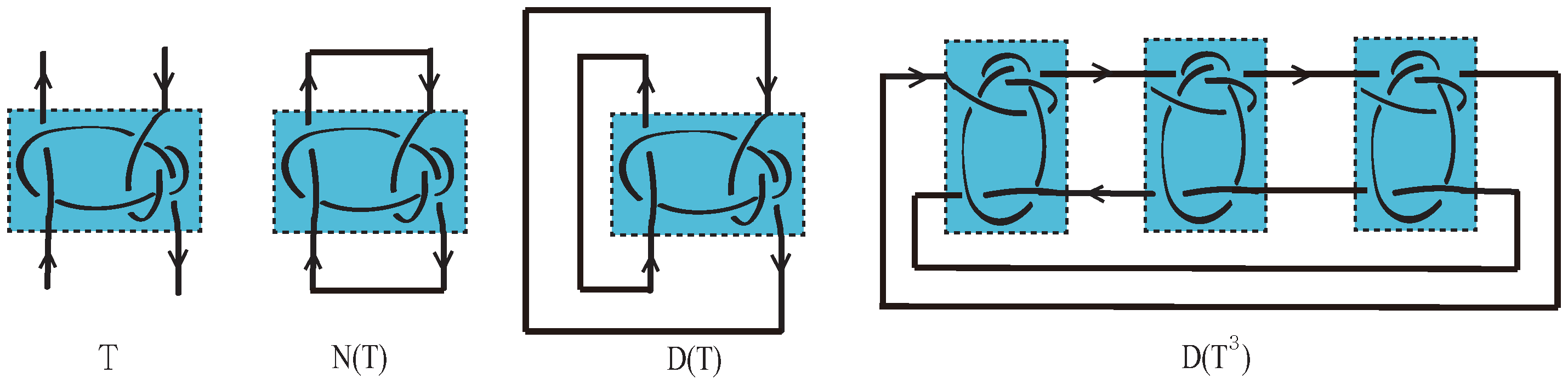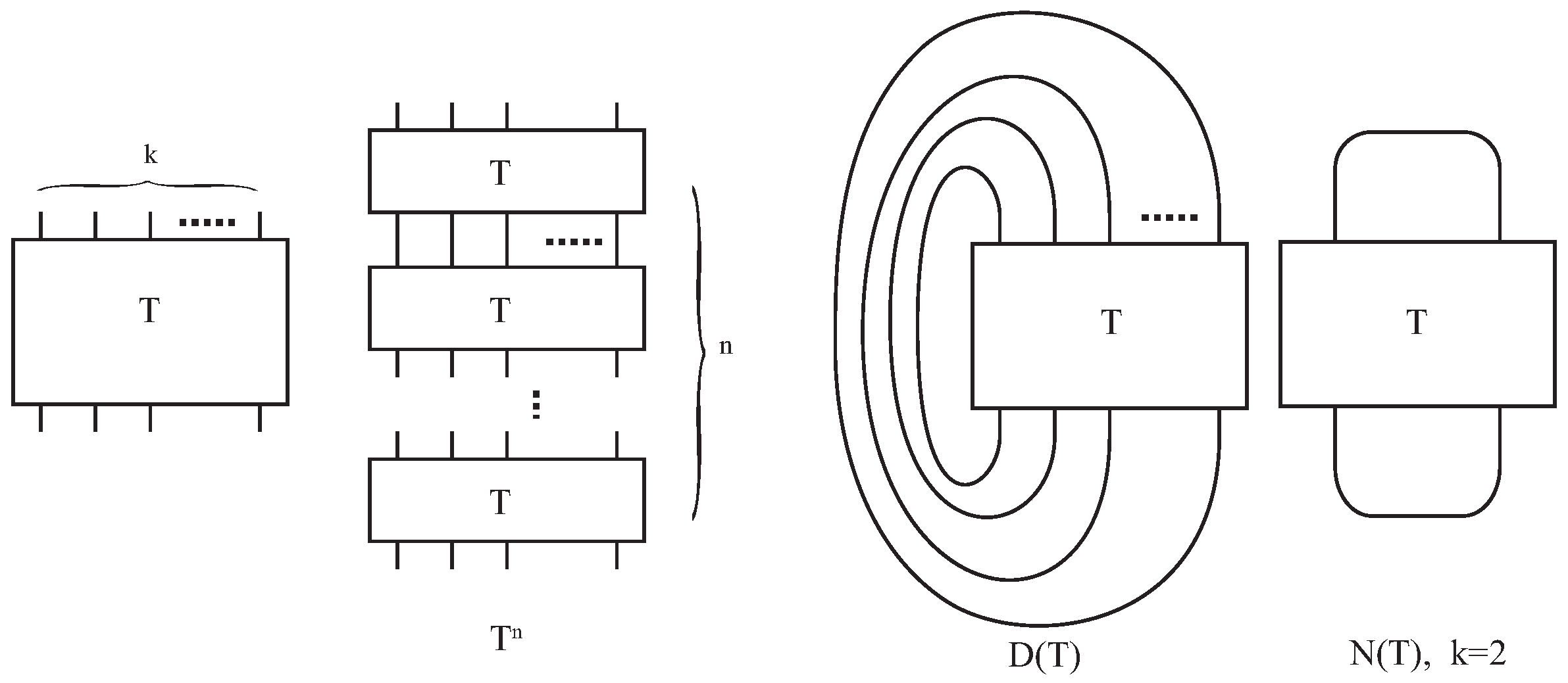By a $2k$-tangle, we mean a $(k,k)$-tangle. Let T be a $2k$-tangle. For an integer $n\ge 2$, let $T^n$ denote the $2k$-tangle obtained by stacking Tn-times. The denominator$D\left(T\right)$ of T is defined by connecting the top ends of T to the bottom ends by parallel lines, see Figure 5. In particular, if T is a 4-tangle, then the numerator $N\left(T\right)$ of T is defined as the last picture in Figure 5. Clearly, $D\left(T^n\right)$ is a periodic link of order n whose factor link is $D\left(T\right)$. If an orientation is given on $D\left(T\right)$, then it induces an orientation of $D\left(T^n\right)$. Notice that every (oriented) periodic link can be constructed in this way.

Figure 5. $(k,k)$-tangle, denominator and numerator.

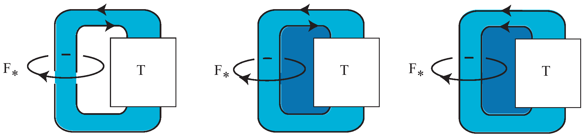
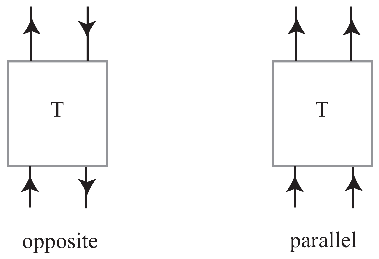
Let T be a 4-tangle and let $D\left(T\right)$ denote the denominator of T which is obtained by connecting the top ends and the bottom ends of T by parallel curves $\alpha$ and $\beta$. Suppose that $D\left(T\right)$ is oriented. Note that the induced orientation at $\alpha$ and $\beta$ are either opposite or parallel, see Figure 6.

Figure 6. Orientation of a tangle.

If the induced orientation at $\alpha$ and $\beta$ are parallel, then $\alpha$ and $\beta$ are contained in different Seifert circles of $D\left(T\right)$. Hence we have the following three cases.

Case I:

The orientations at the end points of the curves in T are opposite and the two outer arcs $\alpha$ and $\beta$ of $D\left(T\right)$ are contained in the same Seifert circle, see the first picture in Figure 7.

Figure 7. Three types of denominator $D\left(T\right)$.

Case II:

The orientations at the end points of the curves in T are opposite and the two outer arcs of $D\left(T\right)$ are contained in different Seifert circles, see the second picture in Figure 7.

Case III:

The orientations at the end points of the curves in T are parallel, see the last picture in Figure 7.

3.1. Periodic Links with Periodicity in Case I

In Case I and Case II, the numerator $N\left(T\right)$ of T is well-defined as an oriented link. In particular, in Case I, the linking number between any Seifert circle of $D\left(T\right)$ and the periodic axis $F_{\ast }$ is always 0, which is equivalent to that $lk(C,F_{\ast })=0$ for any Seifert circle C of $D\left(T\right)$. For Case I, the authors gave the following criteria for Alexander polynomial of the periodic link $D\left(T^n\right)$ by using those of the denominator $D\left(T\right)$ and the numerator $N\left(T\right)$ of a 4-tangle T.

Proposition 2

([2]). Let L be a periodic link of order n with the factor link $L_{\ast }$. Suppose that $L=D\left(T^n\right)$ and $L_{\ast }=D\left(T\right)$ for a 4-tangle T. If $lk(C,F_{\ast })=0$ for any Seifert circle C of $D\left(T\right)$, then the Alexander polynomials of L, $L_{\ast }$ and $N\left(T\right)$ are related as follows;

$$\begin{array}{ccc}\hfill {\mathsf{\Delta }}_L\left(t\right)& =& n{\mathsf{\Delta }}_{L_{\ast }}\left(t\right){\left({\mathsf{\Delta }}_{N\left(T\right)}\left(t\right)\right)}^{n-1}.\hfill \end{array}$$

Indeed, to get the result, the authors showed the following proposition and then applied the determinant formula for the matrix (1).

Proposition 3.

If T is a 4-tangle in Case I, then there exist Seifert matrices $M_{D\left(T\right)},M_{N\left(T\right)},$ and $M_{D\left(T^n\right)}$ of $D\left(T\right),N\left(T\right),$ and $D\left(T^n\right)$, respectively, such that

$$\begin{array}{ccc}\hfill M_{D\left(T\right)}& =& \left(\begin{array}{cc}{M}_{N\left(T\right)}& B\\ C& D\end{array}\right)and\hfill \end{array}$$

$$\begin{array}{ccc}\hfill M_{D\left(T^n\right)}& =& \left(\begin{array}{ccccc}{M}_{N\left(T\right)}& O& \cdots & O& B\\ O& M_{N\left(T\right)}& \cdots & O& B\\ ⋮& ⋮& \ddots & ⋮& ⋮\\ O& O& \cdots & M_{N\left(T\right)}& B\\ C& C& \cdots & C& nD\end{array}\right),\hfill \end{array}$$

where B is a column vector, C is a row vector, O is the zero-matrix and the number of block $M_{N\left(T\right)}$ is n.

3.2. Periodic Links with Periodicity in Case II

In Case II, there is a Seifert circle C of $D\left(T\right)$ such that $lk(C,F_{\ast })\ne 0$. In fact $lk(C_1,F_{\ast })=-lk(C_2,F_{\ast })(=\pm 1)$ where $C_1$ and $C_2$ denote Seifert circles in $D\left(T\right)$ containing $\alpha$ and $\beta$, respectively.

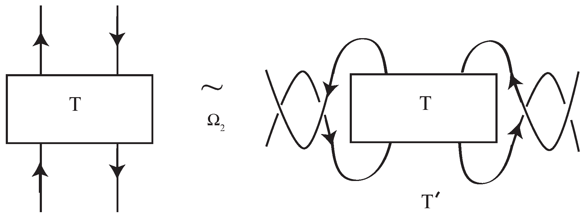
Lemma 1.

If T is a 4-tangle in Case II, then there exist Seifert matrices $M_{D\left(T\right)},M_{N\left(T\right)}$ and $M_{D\left(T^n\right)}$ of $D\left(T\right),N\left(T\right)$ and $D\left(T^n\right)$, respectively, such that

$$\begin{array}{ccc}\hfill M_{N\left(T\right)}& =& \left(\begin{array}{cc}{M}_{D\left(T\right)}& B\\ C& D\end{array}\right)\mathrm{and}\hfill \\ \hfill M_{D\left(T^n\right)}& =& \left(\begin{array}{ccccccccc}{M}_{D\left(T\right)}& O& O& \cdots & O& -B& -B& \cdots & -B\\ O& M_{D\left(T\right)}& O& \cdots & O& B& O& \cdots & O\\ O& O& M_{D\left(T\right)}& \cdots & O& O& B& \cdots & O\\ ⋮& ⋮& ⋮& \ddots & ⋮& ⋮& ⋮& ⋮& ⋮\\ O& O& O& \cdots & M_{D\left(T\right)}& O& O& \cdots & B\\ -C& C& O& \cdots & O& 2D& D& \cdots & D\\ -C& O& C& \cdots & O& D& 2D& \cdots & D\\ ⋮& ⋮& ⋮& \ddots & ⋮& ⋮& ⋮& ⋮& ⋮\\ -C& O& O& \cdots & C& D& D& \cdots & 2D\end{array}\right),\hfill \end{array}$$

where B is a row vector, C is a column vector, O is the zero-matrix, the number of block $M_{D\left(T\right)}$ is n, and the number of block $2D$ is $n-1$ $(n\ge 2)$.

Proof. 

Suppose that the orientations at the end points of the curves in T are opposite and the two outer arcs of $D\left(T\right)$ are contained in different Seifert circles. Without loss of generality, we may assume that T looks like $T^{\prime }$ as seen in Figure 8 that obtained from T by applying the Reidemeister move II between the left two outer curves and the right two outer curves of T, respectively. Note that $D\left(T^{\prime }\right)$, $N\left(T^{\prime }\right)$ and $D\left(T^{\prime n}\right)$ are ambient isotopic to $D\left(T\right)$, $N\left(T\right)$ and $D\left(T^n\right)$, respectively.

Figure 8. Applying Reidemeister Move II.

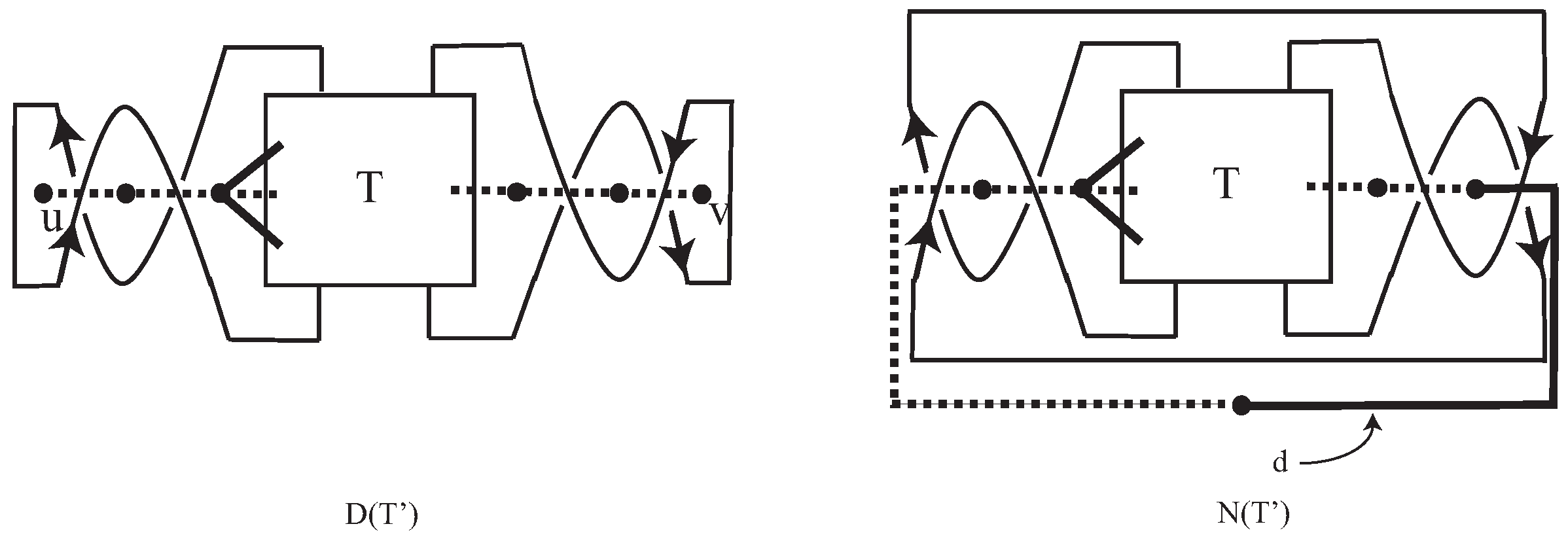
The Seifert graphs ${\mathsf{\Gamma }}_{D\left(T^{\prime }\right)}$ and ${\mathsf{\Gamma }}_{N\left(T^{\prime }\right)}$ of $D\left(T^{\prime }\right)$ and $N\left(T^{\prime }\right)$ are of the form in Figure 9, in which spanning trees ${\tau }_{D\left(T^{\prime }\right)}$ and ${\tau }_{N\left(T^{\prime }\right)}$ of ${\mathsf{\Gamma }}_{D\left(T^{\prime }\right)}$ and ${\mathsf{\Gamma }}_{N\left(T^{\prime }\right)}$ are given by dotted edges in Figure 9. Notice that ${\mathsf{\Gamma }}_{N\left(T^{\prime }\right)}$ is obtained from ${\mathsf{\Gamma }}_{D\left(T^{\prime }\right)}$ by identifying the left vertex u to the right vertex v in ${\mathsf{\Gamma }}_{D\left(T^{\prime }\right)}$ as shown in the right picture in Figure 9. If $E\left({\mathsf{\Gamma }}_{D\left(T^{\prime }\right)}\right)\backslash E\left({\tau }_{D\left(T^{\prime }\right)}\right)=\{e_1,\cdots ,e_k\}$, then $E\left({\mathsf{\Gamma }}_{N\left(T^{\prime }\right)}\right)\backslash E\left({\tau }_{N\left(T^{\prime }\right)}\right)=\{e_1,\cdots ,$$e_k\}\cup \left\{d\right\},$ where d is the new edge of ${\mathsf{\Gamma }}_{D\left(T^{\prime }\right)}$ as shown in Figure 9.

Figure 9. Seifert graphs for $D\left(T\right)$ and $N\left(T\right)$.

The corresponding Seifert matrix $M_{D\left(T^{\prime }\right)}=\left[m_{ij}\left(D\left(T^{\prime }\right)\right)\right]$ of $D\left(T^{\prime }\right)$ is a $k\times k$ matrix, while the Seifert matrix $M_{N\left(T^{\prime }\right)}=\left[m_{ij}\left(N\left(T^{\prime }\right)\right)\right]$ of $N\left(T^{\prime }\right)$ is a $(k+1)\times (k+1)$ matrix. Furthermore, the linking number between $T_{e_i}$ and $T_{e_j}^{+}$ in $N\left(T^{\prime }\right)$ is equal to the linking number between $T_{e_i}$ and $T_{e_j}^{+}$ in $D\left(T^{\prime }\right)$ for all $i,j=1,2,\cdots ,k$, by Proposition 1. Indeed, $m_{ij}\left(D\left(T^{\prime }\right)\right)=m_{ij}\left(N\left(T^{\prime }\right)\right)$ for all $i,j=1,2,\cdots ,k$. Hence the Seifert matrix $M_{N\left(T^{\prime }\right)}$ of $N\left(T^{\prime }\right)$ is given by

$$M_{N\left(T^{\prime }\right)}=\left(\begin{array}{cc}{M}_{D\left(T^{\prime }\right)}& B\\ C& D\end{array}\right),$$

where $B={(lk(T_{e_1},T_d^{+}),\cdots ,lk(T_{e_k},T_d^{+}))}^T,C=(lk(T_d,T_{e_1}^{+}),\cdots ,lk(T_d,T_{e_k}^{+}))$ and $D=lk(T_d,T_d^{+}).$

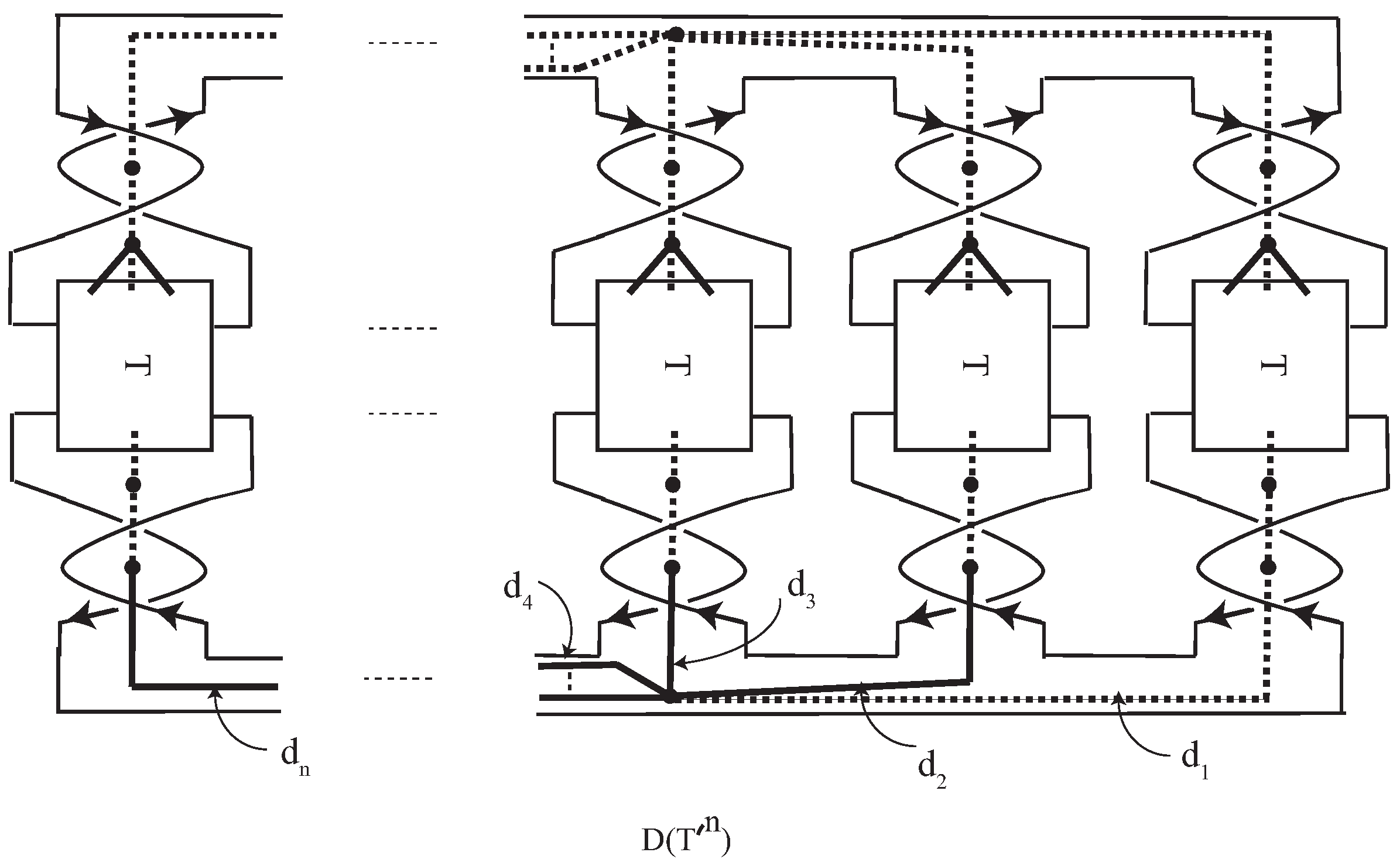
From now on, we will try to find a Seifert matrix $M_{D\left(T^{\prime n}\right)}$ of $D\left(T^{\prime n}\right)$. The Seifert graph ${\mathsf{\Gamma }}_{D\left(T^{\prime n}\right)}$ of $D\left(T^{\prime n}\right)$ consists of n copies of ${\mathsf{\Gamma }}_{D\left(T^{\prime }\right)}$ whose final vertices u and v are used to connect the copies of ${\mathsf{\Gamma }}_{D\left(T^{\prime }\right)}$ as shown in Figure 10. Let $d_p$ be the corresponding pth copy of d for all $p=1,2,\cdots ,n$ in ${\mathsf{\Gamma }}_{D\left(T^{\prime n}\right)}$. By removing $(n-1)$-copies of the edge d, e.g., $d_2,d_3,\cdots ,d_n$ in Figure 10, we get a spanning tree ${\tau }_{D\left(T^{\prime n}\right)}$ of ${\mathsf{\Gamma }}_{D\left(T^{\prime n}\right)}$. Indeed,

$$E({\mathsf{\Gamma }}_{D\left(T^{\prime n}\right)})\backslash E\left(\tau \left(D\left(T^{\prime n}\right)\right)\right)={\cup }_{p=1}^n\{e_1^p,\cdots ,e_k^p\}\cup \{d_2,d_3,\cdots ,d_n\},$$

where $\{e_1^p,\cdots ,e_k^p\}$ is the corresponding pth copy of $\{e_1,\cdots ,e_k\}$.

Figure 10. Seifert graph for $D\left(T^n\right)$.

Since the linking number between $T_{e_i^p}$ and $T_{e_j^p}^{+}$ in $D\left(T^{\prime n}\right)$ is equal to the linking number between $T_{e_i}$ and $T_{e_j}^{+}$ in $D\left(T^{\prime }\right)$ for all $i,j=1,2,\cdots ,k$ and $p=1,\cdots ,n,$ we have $m_{i^p{j}^p}\left(D\left(T^{\prime n}\right)\right)=m_{ij}(D\left(T^{\prime }\right)),$ where $m_{i^p{j}^p}\left(D\left(T^{\prime n}\right)\right)=lk(T_{e_i^p},T_{e_j^p}^{+})$. If $p\ne q$, since $T_{e_i^p}$ and $T_{e_j^q}$ do not intersect, $m_{i^p{j}^q}\left(D\left(T^{\prime n}\right)\right)=0$ for all $i,j=1,2,\cdots ,k,$ by Proposition 1. Hence,

$$m_{i^p{j}^q}\left(D\left(T^{\prime n}\right)\right)=\left\{\begin{array}{cc}{m}_{ij}\left(D\left(T^{\prime }\right)\right),\hfill & \mathrm{if}p=q;\hfill \\ 0,\hfill & \mathrm{if}p\ne q.\hfill \end{array}\right.$$

On the other hand, since $T_{d_p}$ lies in the 1st copy and pth copy of $T_{e_i}\cap T_{d_p}$, we have $lk(T_{e_i^1},T_{d_p}^{+})=-lk(T_{e_i},T_d^{+})=-B$, $lk(T_{d_p},T_{e_i^1}^{+})=-lk(T_d,T_{e_i}^{+})=-C$, $lk(T_{e_i^p},T_{d_p}^{+})=lk(T_{e_i},T_d^{+})=B$ and $lk(T_{d_p},T_{e_i^p}^{+})=lk(T_d,T_{e_i}^{+})=C$ for all $p=2,3,\cdots ,n$. For $p\ne q$ and $p,q=2,3,\cdots ,n$, $lk(T_{e_i^p},T_{d_q}^{+})=0$ and $lk(T_{d_q},T_{e_i^p}^{+})=0$ since $T_{e_i^p}$ and $T_{d_q}$ do not intersect in $D\left(T^{\prime n}\right)$.

Since T is connected, the generator $T_{d_p}$ runs through 2 copies, in each of which the self linking number of $T_d$ is equal to D for all $p=2,3,\cdots ,n$. Furthermore, since the orientations at the end points of the curves in T are opposite, D is even. Hence, $lk(T_{d_p},T_{d_p}^{+})=2·lk(T_d,T_d^{+})=2D$ for all $p=2,3,\cdots ,n$, by Proposition 1. For all $p,q=2,3,\cdots ,n$ and $p\ne q$, $lk(T_{d_p},T_{d_q}^{+})=lk(T_d,T_d^{+})=D.$ Because generators $T_{d_p}$ and $T_{d_q}$ meet in the just 1st copy. ☐

Hence by using Theorem 1, we get the following result.

Theorem 3.

Let L be a periodic link of order n $(n\ge 2)$ with the factor link $L_{\ast }$. Suppose that $L=D\left(T^n\right)$ and $L_{\ast }=D\left(T\right)$ for a 4-tangle T in Case II. Then the Alexander polynomials of $D\left(T^n\right)$, $D\left(T\right)$ and $N\left(T\right)$ are related as follows;

$${\mathsf{\Delta }}_L\left(t\right)=n{\mathsf{\Delta }}_{L_{\ast }}\left(t\right){\left({\mathsf{\Delta }}_{N\left(T\right)}\left(t\right)\right)}^{n-1}.$$

Proof. 

By the definition of the Alexander polynomial of a link and by Lemma 1, we have

$$\begin{array}{ccc}\hfill {\mathsf{\Delta }}_{N\left(T\right)}\left(t\right)& =& det\left(\begin{array}{cc}{t}^{\frac{1}{2}}{M}_{D\left(T\right)}-t^{-\frac{1}{2}}{M_{D\left(T\right)}}^T& t^{\frac{1}{2}}B-t^{-\frac{1}{2}}{C}^T\\ t^{\frac{1}{2}}C-t^{-\frac{1}{2}}{B}^T& (t^{\frac{1}{2}}-t^{-\frac{1}{2}})D\end{array}\right),\hfill \\ \hfill {\mathsf{\Delta }}_{D\left(T^n\right)}\left(t\right)& =& ndet(t^{\frac{1}{2}}{M}_{D\left(T\right)}-t^{-\frac{1}{2}}{M_{D\left(T\right)}}^T)\hfill \\ & & \times det{\left(\begin{array}{cc}{t}^{\frac{1}{2}}{M}_{D\left(T\right)}-t^{-\frac{1}{2}}{M_{D\left(T\right)}}^T& t^{\frac{1}{2}}B-t^{-\frac{1}{2}}{C}^T\\ t^{\frac{1}{2}}C-t^{-\frac{1}{2}}{B}^T& (t^{\frac{1}{2}}-t^{-\frac{1}{2}})D\end{array}\right)}^{n-1}\hfill \\ & =& n{\mathsf{\Delta }}_{D\left(T\right)}\left(t\right){\left({\mathsf{\Delta }}_{N\left(T\right)}\left(t\right)\right)}^{n-1}.\hfill \end{array}$$

☐

Since the result in Theorem 3 (Case II) equals that in Proposition 2 (Case I), we can summarize them as

Theorem 4.

Let L be a periodic link of order n $(n\ge 2)$ with the factor link $L_{\ast }$. Suppose that $L=D\left(T^n\right)$ and $L_{\ast }=D\left(T\right)$ for a 4-tangle T whose numerator $N\left(T\right)$ is defined. Then the Alexander polynomials of L, $L_{\ast }$ and $N\left(T\right)$ are related as follows;

$${\mathsf{\Delta }}_L\left(t\right)=n{\mathsf{\Delta }}_{L_{\ast }}\left(t\right){\left({\mathsf{\Delta }}_{N\left(T\right)}\left(t\right)\right)}^{n-1}.$$

Theorem 5.

Let L be a periodic link of order n $(n\ge 2)$ with the factor link $L_{\ast }$. Suppose that $L=D\left(T^n\right)$ and $L_{\ast }=D\left(T\right)$ for a 4-tangle T whose numerator $N\left(T\right)$ is defined. Then the determinants of L, $L_{\ast }$ and $N\left(T\right)$ are related as follows;

$$det\left(L\right)=ndet\left(L_{\ast }\right){\{det\left(N\left(T\right)\right)\}}^{n-1}.$$

Proof. 

Note that $det\left(L\right)=|{\mathsf{\Delta }}_L(-1)|$ for any oriented link L. By Theorem 4, we have

$$\begin{array}{ccc}\hfill detD\left(T^n\right)& =& |{\mathsf{\Delta }}_{D\left(T^n\right)}(-1)|\hfill \\ & =& |n{\mathsf{\Delta }}_{D\left(T\right)}(-1){\left\{{\mathsf{\Delta }}_{N\left(T\right)}(-1)\right\}}^{n-1}|\hfill \\ & =& n|{\mathsf{\Delta }}_{D\left(T\right)}(-1)||\left\{{\mathsf{\Delta }}_{N\left(T\right)}(-1)\right\}{|}^{n-1}\hfill \\ & =& ndet\left(D\left(T\right)\right){\{detN\left(T\right)\}}^{n-1}.\hfill \end{array}$$

☐

Example 1.

Consider the oriented 4-tangle T in Figure 11, which is a 4-tangle in Case II.

Figure 11. Example for Case II.

The Seifert matrices of $N\left(T\right)$ and $D\left(T\right)$ are given by

$$M_{D\left(T\right)}=\left(\begin{array}{ccc}\hfill -1& \hfill 0& \hfill 0\\ \hfill 0& \hfill -1& \hfill -1\\ \hfill 0& \hfill 0& \hfill -2\end{array}\right)and{M}_{N\left(T\right)}=\left(\begin{array}{cccc}\hfill -1& \hfill 0& \hfill 0& \hfill 0\\ \hfill 0& \hfill -1& \hfill -1& \hfill 0\\ \hfill 0& \hfill 0& \hfill -2& \hfill -1\\ \hfill -1& \hfill -1& \hfill -1& \hfill -2\end{array}\right),$$

while

$$M_{D\left(T^3\right)}=\left(\begin{array}{ccccccccccc}\hfill -1& \hfill 0& \hfill 0& \hfill 0& \hfill 0& \hfill 0& \hfill 0& \hfill 0& \hfill 0& \hfill 0& \hfill 0\\ \hfill 0& \hfill -1& \hfill -1& \hfill 0& \hfill 0& \hfill 0& \hfill 0& \hfill 0& \hfill 0& \hfill 0& \hfill 0\\ \hfill 0& \hfill 0& \hfill -2& \hfill 0& \hfill 0& \hfill 0& \hfill 0& \hfill 0& \hfill 0& \hfill 1& \hfill 1\\ \hfill 0& \hfill 0& \hfill 0& \hfill -1& \hfill 0& \hfill 0& \hfill 0& \hfill 0& \hfill 0& \hfill 0& \hfill 0\\ \hfill 0& \hfill 0& \hfill 0& \hfill 0& \hfill -1& \hfill -1& \hfill 0& \hfill 0& \hfill 0& \hfill 0& \hfill 0\\ \hfill 0& \hfill 0& \hfill 0& \hfill 0& \hfill 0& \hfill -2& \hfill 0& \hfill 0& \hfill 0& \hfill -1& \hfill 0\\ \hfill 0& \hfill 0& \hfill 0& \hfill 0& \hfill 0& \hfill 0& \hfill -1& \hfill 0& \hfill 0& \hfill 0& \hfill 0\\ \hfill 0& \hfill 0& \hfill 0& \hfill 0& \hfill 0& \hfill 0& \hfill 0& \hfill -1& \hfill -1& \hfill 0& \hfill 0\\ \hfill 0& \hfill 0& \hfill 0& \hfill 0& \hfill 0& \hfill 0& \hfill 0& \hfill 0& \hfill -2& \hfill 0& \hfill -1\\ \hfill 1& \hfill 1& \hfill 1& \hfill -1& \hfill -1& \hfill -1& \hfill 0& \hfill 0& \hfill 0& \hfill -4& \hfill -2\\ \hfill 1& \hfill 1& \hfill 1& \hfill 0& \hfill 0& \hfill 0& \hfill -1& \hfill -1& \hfill -1& \hfill -2& \hfill -4\end{array}\right).$$

By the direct calculation, one can see that the Alexander polynomials of $D\left(T\right)$ and $N\left(T\right)$ are

$$\begin{array}{ccc}\hfill {\mathsf{\Delta }}_{D\left(T\right)}\left(t\right)& =& -2t^{\frac{3}{2}}+5t^{\frac{1}{2}}-5t^{-\frac{1}{2}}+2t^{-\frac{3}{2}}\mathrm{and}\hfill \\ \hfill {\mathsf{\Delta }}_{N\left(T\right)}\left(t\right)& =& 4t^2-8t+9-8t^{-1}+4t^{-2}.\hfill \end{array}$$

By using Theorem 3, we get the Alexander polynomial of $D\left(T^3\right)$;

$$\begin{array}{ccc}\hfill {\mathsf{\Delta }}_{D\left(T^3\right)}\left(t\right)& =& 3(-2t^{\frac{3}{2}}+5t^{\frac{1}{2}}-5t^{-\frac{1}{2}}+2t^{-\frac{3}{2}}){(4t^2-8t+9-8t^{-1}+4t^{-2})}^2\hfill \\ & =& -96t^{\frac{11}{2}}+624t^{\frac{9}{2}}-2016t^{\frac{7}{2}}+4344t^{\frac{5}{2}}-6990t^{\frac{3}{2}}+8799t^{\frac{1}{2}}-8799t^{-\frac{1}{2}}\hfill \\ & & +6990t^{-\frac{3}{2}}-4344t^{\frac{5}{2}}+2016t^{-\frac{7}{2}}-624t^{-\frac{9}{2}}+96t^{-\frac{11}{2}}.\hfill \end{array}$$

Finally, one can get $det\left(D\left(T^3\right)\right)=3\left(14\right){\left(33\right)}^2=45738$ by Theorem 5 because $det\left(D\right(T\left)\right)=14$ and $det\left(N\right(T\left)\right)=33$.

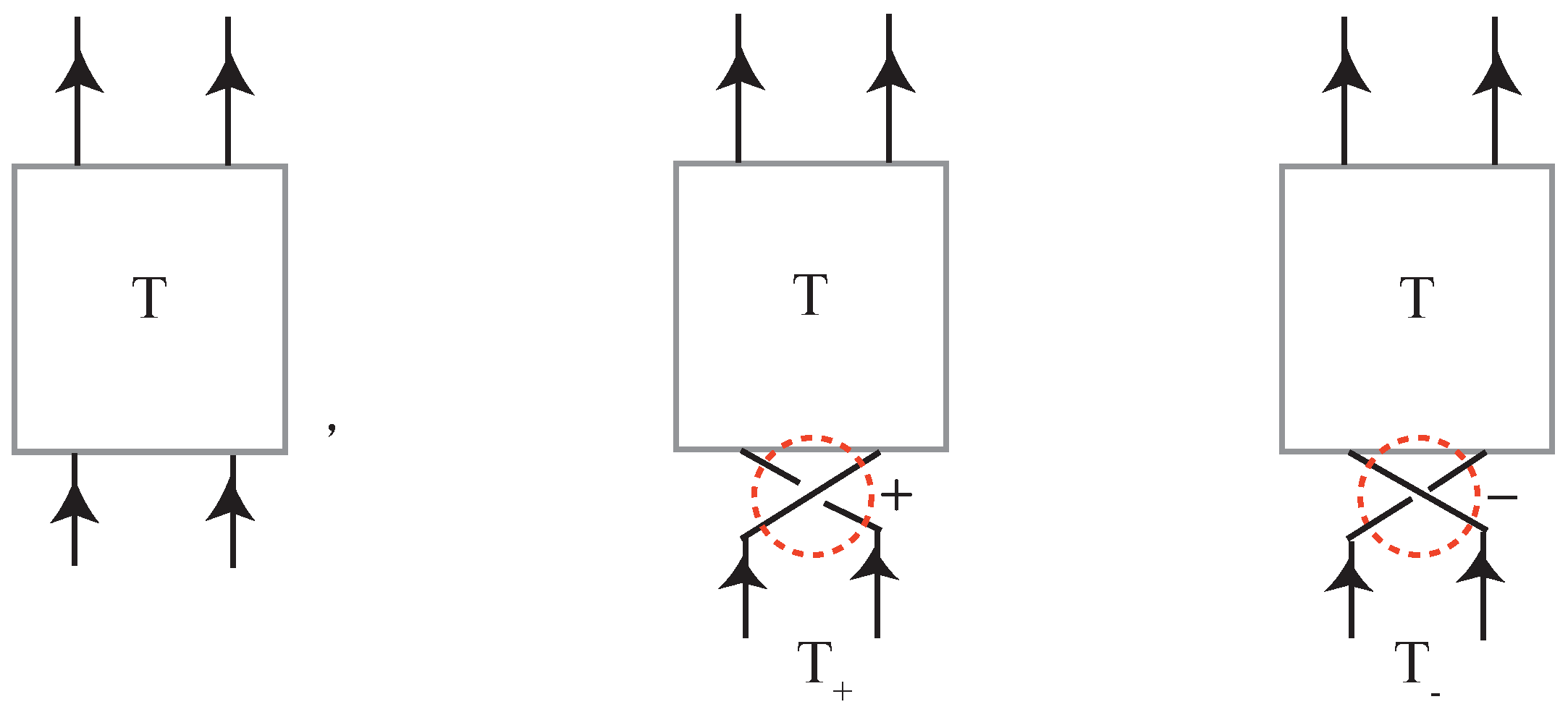
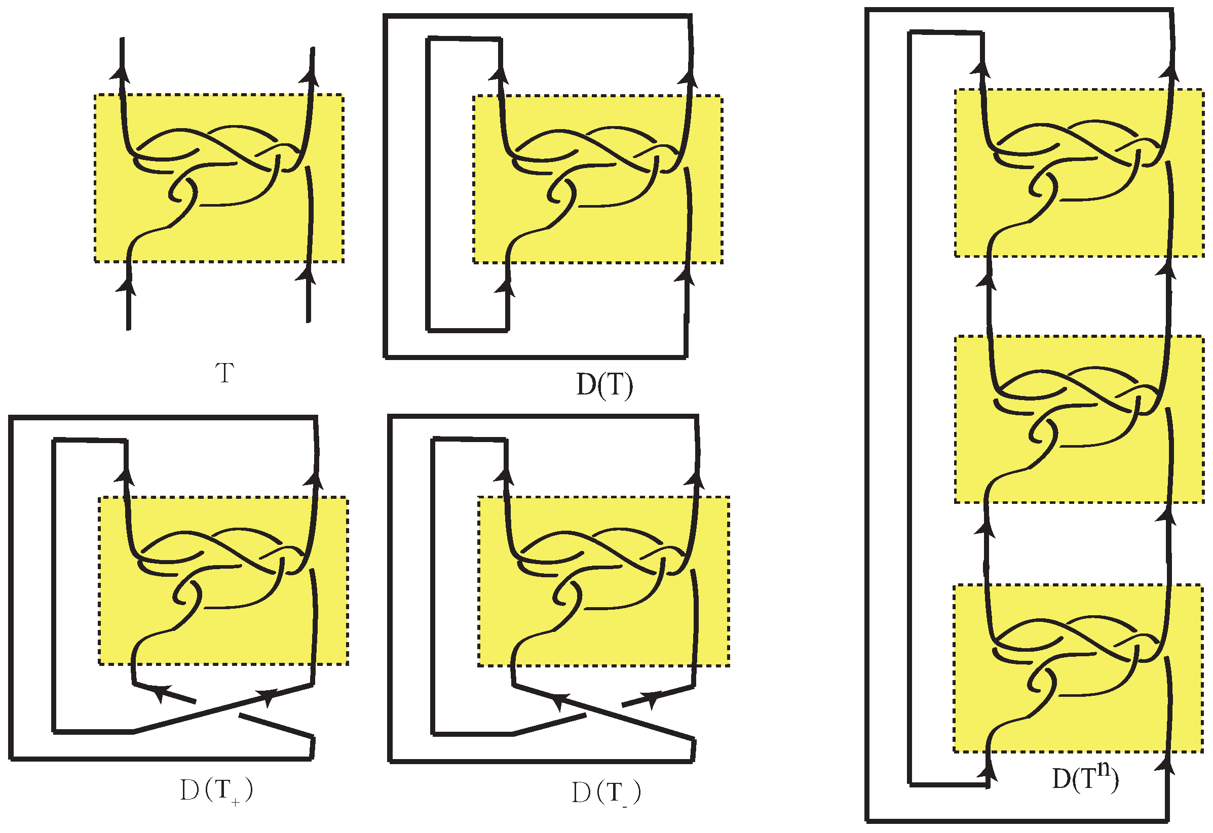
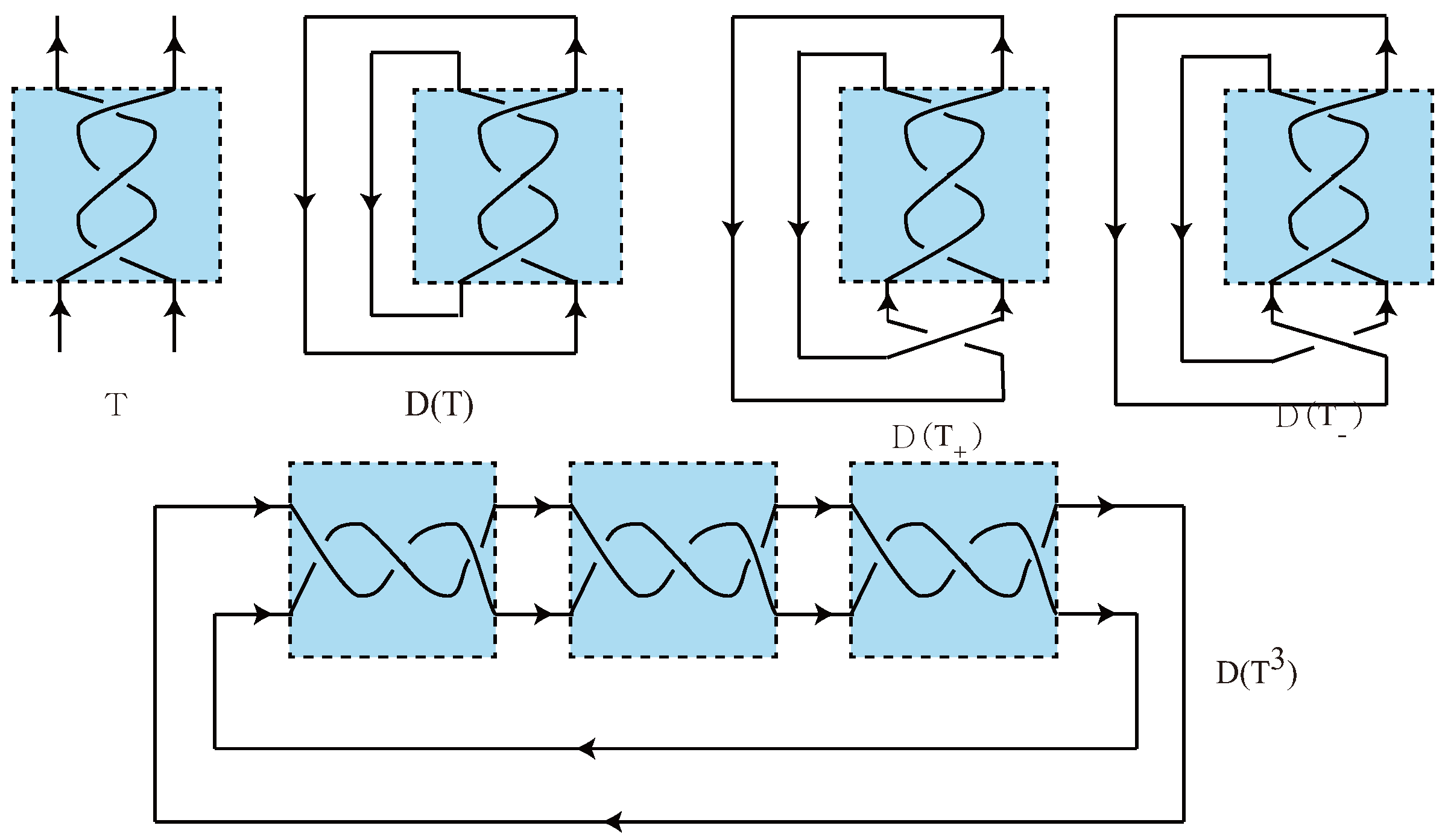
3.3. Periodic Links with Periodicity in Case III

In Case III, recall that the orientation of T is given as the left of Figure 12 so that there exist exactly two Seifert circles $C_1$ and $C_2$ in $D\left(T\right)$ such that $lk(C_1,F_{\ast })=lk(C_2,F_{\ast })(=\pm 1)$. Note that the orientation of T cannot be extended to an orientation of $N\left(T\right)$. Define $T_{+}$ and $T_{-}$ by adding a positive crossing and a negative crossing at the bottom of T respectively, as shown in Figure 12.

Figure 12. T₊ and T₋.

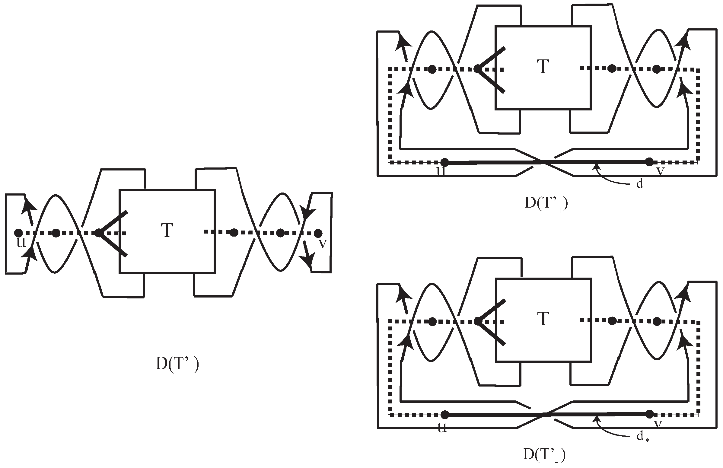
Lemma 2.

If T is a 4-tangle in Case III, then there exist Seifert matrices $M_{D\left(T\right)},M_{D\left(T_{+}\right)},M_{D\left(T_{-}\right)}$ and $M_{D\left(T^n\right)}$ of $D\left(T\right),D\left(T_{+}\right),D\left(T_{-}\right)$ and $D\left(T^n\right)$, respectively, such that

$$\begin{array}{ccc}\hfill M_{D\left(T_{+}\right)}& =& \left(\begin{array}{cc}{M}_{D\left(T\right)}& B\\ C& D\end{array}\right),\hfill \\ \hfill M_{D\left(T_{-}\right)}& =& \left(\begin{array}{cc}{M}_{D\left(T\right)}& B\\ C& E\end{array}\right)\mathrm{and}\hfill \\ \hfill M_{D\left(T^n\right)}& =& \left(\begin{array}{ccccccccc}{M}_{D\left(T\right)}& O& O& \cdots & O& -B& -B& \cdots & -B\\ O& M_{D\left(T\right)}& O& \cdots & O& B& O& \cdots & O\\ O& O& M_{D\left(T\right)}& \cdots & O& O& B& \cdots & O\\ ⋮& ⋮& ⋮& \ddots & ⋮& ⋮& ⋮& \ddots & ⋮\\ O& O& O& \cdots & M_{D\left(T\right)}& O& O& \cdots & B\\ -C& C& O& \cdots & O& D+E& D& \cdots & D\\ -C& O& C& \cdots & O& E& D+E& \cdots & D\\ ⋮& ⋮& ⋮& \ddots & ⋮& ⋮& ⋮& \ddots & ⋮\\ -C& O& O& \cdots & C& E& E& \cdots & D+E\end{array}\right),\hfill \end{array}$$

where B is a row vector, C is a column vector, O is the zero-matrix, $E=D+1$, the number of block $M_{D\left(T\right)}$ is n and the number of block $(D+E)$ is $n-1$.

Proof. 

Since the process of the proof is similar to that of Theorem 3, we will give briefly sketch of the proof.

The Seifert graphs ${\mathsf{\Gamma }}_{D\left(T^{\prime }\right)}$, ${\mathsf{\Gamma }}_{D\left(T_{+}^{\prime }\right)}$ and ${\mathsf{\Gamma }}_{D\left(T_{-}^{\prime }\right)}$ of $D\left(T^{\prime }\right)$, $D\left(T_{+}^{\prime }\right)$ and $D\left(T_{-}^{\prime }\right)$ are of the form in Figure 13, in which spanning trees ${\tau }_{D\left(T^{\prime }\right)}$, ${\tau }_{D\left(T_{+}^{\prime }\right)}$ and ${\tau }_{D\left(T_{-}^{\prime }\right)}$ of ${\mathsf{\Gamma }}_{D\left(T^{\prime }\right)}$ ${\mathsf{\Gamma }}_{D\left(T_{+}^{\prime }\right)}$ and ${\mathsf{\Gamma }}_{D\left(T_{-}^{\prime }\right)}$ are given by dotted edges in Figure 13.

Figure 13. Seifert graphs of $D\left(T^{\prime }\right)$, $D\left(T_{+}^{\prime }\right)$ and $D\left(T_{-}^{\prime }\right)$.

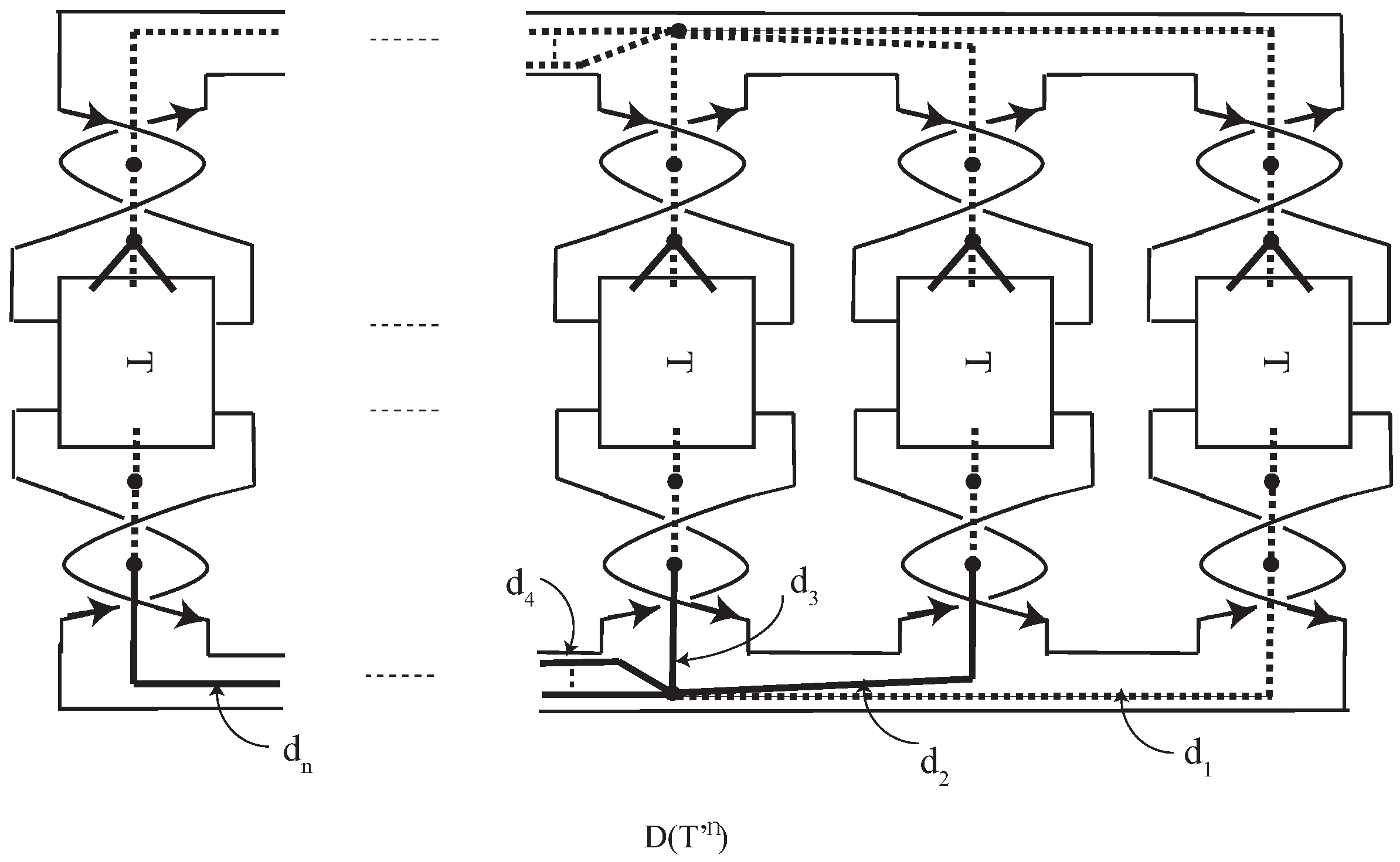
The Seifert graph ${\mathsf{\Gamma }}_{D\left(T^{\prime n}\right)}$ of $D\left(T^{\prime n}\right)$ consists of n copies of ${\mathsf{\Gamma }}_{D\left(T^{\prime }\right)}$ whose the end vertices u and v are used to connect the copies of ${\mathsf{\Gamma }}_{D\left(T^{\prime }\right)}$ as shown in Figure 14. Let $d_p$ be the corresponding pth copy of d for all $p=1,2,\cdots ,n$ in $D\left(T^{\prime n}\right)$. Notice that by the construction of $D\left(T^{\prime n}\right)$, d and $d_{\ast }$ correspond to the same edge in $D\left(T^{\prime n}\right)$, where d and $d_{\ast }$ were new edges in Figure 13. By removing $(n-1)$-copies of the edge d (or $d_{\ast }$) in ${\mathsf{\Gamma }}_{D\left(T^{\prime }\right)}$, e.g., $d_2,d_3,\cdots ,d_n$ in Figure 14, we get a spanning tree ${\tau }_{D\left(T^{\prime n}\right)}$ of $D\left(T^{\prime n}\right)$. ☐

Figure 14. Seifert graph of $D\left(T^{\prime n}\right)$.

By using the determinant formula in Theorem 2, we get the following theorem.

Theorem 6.

Let L be a periodic link of order n $(n\ge 2)$ with the factor link $L_{\ast }$. Suppose that $L=D\left(T^n\right)$ and $L_{\ast }=D\left(T\right)$ for a 4-tangle T in Case III. Then the Alexander polynomials of L, $L_{\ast }$, $D\left(T_{+}\right)$ and $D\left(T_{-}\right)$ are related as follows;

$$\begin{array}{ccc}\hfill {\mathsf{\Delta }}_L\left(t\right)& =& {\mathsf{\Delta }}_{L_{\ast }}\left(t\right)\sum _{k=1}^n{\left({\mathsf{\Delta }}_{D\left(T_{+}\right)}\left(t\right)\right)}^{n-k}{\left({\mathsf{\Delta }}_{D\left(T_{-}\right)}\left(t\right)\right)}^{k-1}.\hfill \end{array}$$

Proof. 

By the definition of the Alexander polynomial of a link and by Lemma 2, we have

$$\begin{array}{ccc}\hfill {\mathsf{\Delta }}_{D\left(T_{+}\right)}\left(t\right)& =& det\left(\begin{array}{cc}{t}^{\frac{1}{2}}{M}_{D\left(T\right)}-t^{-\frac{1}{2}}{M_{D\left(T\right)}}^T& t^{\frac{1}{2}}B-t^{-\frac{1}{2}}{C}^T\\ t^{\frac{1}{2}}C-t^{-\frac{1}{2}}{B}^T& (t^{\frac{1}{2}}-t^{-\frac{1}{2}})D\end{array}\right),\hfill \\ \hfill {\mathsf{\Delta }}_{D\left(T_{-}\right)}\left(t\right)& =& det\left(\begin{array}{cc}{t}^{\frac{1}{2}}{M}_{D\left(T\right)}-t^{-\frac{1}{2}}{M_{D\left(T\right)}}^T& t^{\frac{1}{2}}B-t^{-\frac{1}{2}}{C}^T\\ t^{\frac{1}{2}}C-t^{-\frac{1}{2}}{B}^T& (t^{\frac{1}{2}}-t^{-\frac{1}{2}})E\end{array}\right),\hfill \end{array}$$

$$\begin{array}{ccc}\hfill {\mathsf{\Delta }}_{D\left(T^n\right)}\left(t\right)& =& det(t^{\frac{1}{2}}{M}_{D\left(T\right)}-t^{-\frac{1}{2}}{M_{D\left(T\right)}}^T)\hfill \\ & & \times \sum _{k=1}^n[{\left\{det\left(\begin{array}{cc}{t}^{\frac{1}{2}}{M}_{D\left(T\right)}-t^{-\frac{1}{2}}{M_{D\left(T\right)}}^T& t^{\frac{1}{2}}B-t^{-\frac{1}{2}}{C}^T\\ t^{\frac{1}{2}}C-t^{-\frac{1}{2}}{B}^T& (t^{\frac{1}{2}}-t^{-\frac{1}{2}})D\end{array}\right)\right\}}^{n-k}\hfill \\ & & \times {\left\{det\left(\begin{array}{cc}{t}^{\frac{1}{2}}{M}_{D\left(T\right)}-t^{-\frac{1}{2}}{M_{D\left(T\right)}}^T& t^{\frac{1}{2}}B-t^{-\frac{1}{2}}{C}^T\\ t^{\frac{1}{2}}C-t^{-\frac{1}{2}}{B}^T& (t^{\frac{1}{2}}-t^{-\frac{1}{2}})E\end{array}\right)\right\}}^{k-1}]\hfill \\ & =& {\mathsf{\Delta }}_{D\left(T\right)}\left(t\right)\sum _{k=1}^n{\left\{{\mathsf{\Delta }}_{D\left(T_{+}\right)}\left(t\right)\right\}}^{n-k}{\left\{{\mathsf{\Delta }}_{D\left(T_{-}\right)}\left(t\right)\right\}}^{k-1}.\hfill \end{array}$$

☐

In general, the determinant of $D\left(T^n\right)$ cannot be calculated by using Theorem 6 because $\left|det(A+B)\right|\ne \left|detA\right|+\left|detB\right|$. But we can calculate the determinant of $D\left(T^n\right)$ under certain conditions.

Theorem 7.

Let L be a periodic link of order n $(n\ge 2)$ with the factor link $L_{\ast }$. Suppose that $L=D\left(T^n\right)$ and $L_{\ast }=D\left(T\right)$ for a 4-tangle T in Case III. If ${(-1)}^{m+1}{\mathsf{\Delta }}_{D\left(T_{+}\right)}(-1)·{\mathsf{\Delta }}_{D\left(T_{-}\right)}(-1)\ge 0$, then

$$det\left(D\left(T^n\right)\right)=det\left(D\left(T\right)\right)\sum _{k=1}^n{\left\{det\left(D\left(T_{+}\right)\right)\right\}}^{n-k}{\left\{det\left(D\left(T_{-}\right)\right)\right\}}^{k-1},$$

where m is the size of a Seifert matrix of $D\left(T\right)$.

Proof. 

Notice that, ${\mathsf{\Delta }}_L(-1)=i^{m}det(M+M^T)$ for a Seifert matrix $M_{m\times m}$ of a link L.

From the definition of the determinant of a link, Theorem 2 and Lemma 2, if the Seifert matrix $M_{D\left(T\right)}$ of $D\left(T\right)$ is an $m\times m$ matrix and ${(-1)}^{m+1}{\mathsf{\Delta }}_{D\left(T_{+}\right)}(-1)·{\mathsf{\Delta }}_{D\left(T_{-}\right)}(-1)\ge 0$, then the determinant of $D\left(T^n\right)$ is

$$\begin{array}{cc}& |det({(-1)}^{\frac{1}{2}}{M}_{D\left(T\right)}-{(-1)}^{-\frac{1}{2}}{M_{D\left(T\right)}}^T)\hfill \\ & \times \sum _{k=1}^n[{\left\{det\left(\begin{array}{cc}{(-1)}^{\frac{1}{2}}{M}_{D\left(T\right)}-{(-1)}^{-\frac{1}{2}}{M_{D\left(T\right)}}^T& {(-1)}^{\frac{1}{2}}B-{(-1)}^{-\frac{1}{2}}{C}^T\\ {(-1)}^{\frac{1}{2}}C-{(-1)}^{-\frac{1}{2}}{B}^T& ({(-1)}^{\frac{1}{2}}-{(-1)}^{-\frac{1}{2}})D\end{array}\right)\right\}}^{n-k}\hfill \\ & \times {\left\{\left(\begin{array}{cc}{(-1)}^{\frac{1}{2}}{M}_{D\left(T\right)}-{(-1)}^{-\frac{1}{2}}{M_{D\left(T\right)}}^T& {(-1)}^{\frac{1}{2}}B-{(-1)}^{-\frac{1}{2}}{C}^T\\ {(-1)}^{\frac{1}{2}}C-{(-1)}^{-\frac{1}{2}}{B}^T& ({(-1)}^{\frac{1}{2}}-{(-1)}^{-\frac{1}{2}})E\end{array}\right)\right\}}^{k-1}]|\hfill \\ =& |{\mathsf{\Delta }}_{D\left(T\right)}(-1)|\times |\sum _{k=1}^n{\left\{{\mathsf{\Delta }}_{D\left(T_{+}\right)}(-1)\right\}}^{n-k}{\left\{{\mathsf{\Delta }}_{D\left(T_{-1}\right)}(-1)\right\}}^{k-1}|\hfill \\ =& |{\mathsf{\Delta }}_{D\left(T\right)}(-1)|\times |\sum _{k=1}^n{\{i^{m+1}det(M_{D\left(T_{+}\right)}+{M_{D\left(T_{+}\right)}}^T)\}}^{n-k}{\{i^{m+1}det(M_{D\left(T_{-}\right)}+{M_{D\left(T_{-}\right)}}^T)\}}^{k-1}|\hfill \\ =& |{\mathsf{\Delta }}_{D\left(T\right)}(-1)|\times |\sum _{k=1}^n{\{det(M_{D\left(T_{+}\right)}+{M_{D\left(T_{+}\right)}}^T)\}}^{n-k}{\{det(M_{D\left(T_{-}\right)}+{M_{D\left(T_{-}\right)}}^T)\}}^{k-1}|\hfill \\ \begin{array}{c}=\\ \left(1\right)\end{array}& |{\mathsf{\Delta }}_{D\left(T\right)}(-1)|\sum _{k=1}^n|det(M_{D\left(T_{+}\right)}+{M_{D\left(T_{+}\right)}}^T){|}^{n-k}{|det(M_{D\left(T_{-}\right)}+{M_{D\left(T_{-}\right)}}^T)|}^{k-1}\hfill \\ =& det\left(D\left(T\right)\right)\sum _{k=1}^n{\left\{det\left(D\left(T_{+}\right)\right)\right\}}^{n-k}{\left\{det\left(D\left(T_{-}\right)\right)\right\}}^{k-1}.\hfill \end{array}$$

The identity (1) comes by the condition ${(-1)}^{m+1}{\mathsf{\Delta }}_{D\left(T_{+}\right)}(-1)·{\mathsf{\Delta }}_{D\left(T_{-}\right)}(-1)\ge 0$ because

$$\begin{array}{cc}& det(M_{D\left(T_{+}\right)}+{M_{D\left(T_{+}\right)}}^T)det(M_{D\left(T_{-}\right)}+{M_{D\left(T_{-}\right)}}^T)\ge 0\hfill \\ \iff & {\left(i\right)}^{-(m+1)}{\mathsf{\Delta }}_{D\left(T_{+}\right)}(-1)·{\left(i\right)}^{-(m+1)}{\mathsf{\Delta }}_{D\left(T_{-}\right)}(-1)\ge 0\hfill \\ \iff & {(-1)}^{m+1}{\mathsf{\Delta }}_{D\left(T_{+}\right)}(-1)·{\mathsf{\Delta }}_{D\left(T_{-}\right)}(-1)\ge 0.\hfill \end{array}$$

☐

Example 2.

Consider the oriented 4-tangle T in Figure 15, which is a 4-tangle in Case III.

Figure 15. Example for Case III.

The Seifert matrices of $D\left(T\right)$, $D\left(T_{+}\right)$ and $D\left(T_{-}\right)$ are given by

$$M_{D\left(T\right)}=\left(\begin{array}{cccc}\hfill 1& \hfill 0& \hfill 0& \hfill 0\\ \hfill -1& \hfill 1& \hfill 0& \hfill 0\\ \hfill -1& \hfill 0& \hfill 1& \hfill 0\\ \hfill 0& \hfill 0& \hfill 1& \hfill 1\end{array}\right),M_{D\left(T_{+}\right)}=\left(\begin{array}{ccccc}\hfill 1& \hfill 0& \hfill 0& \hfill 0& \hfill 0\\ \hfill -1& \hfill 1& \hfill 0& \hfill 0& \hfill 1\\ \hfill -1& \hfill 0& \hfill 1& \hfill 0& \hfill 1\\ \hfill 0& \hfill 0& \hfill 1& \hfill 1& \hfill 1\\ \hfill 0& \hfill 0& \hfill 0& \hfill 0& \hfill 0\end{array}\right)\mathrm{and}{M}_{D\left(T_{-}\right)}=\left(\begin{array}{ccccc}\hfill 1& \hfill 0& \hfill 0& \hfill 0& \hfill 0\\ \hfill -1& \hfill 1& \hfill 0& \hfill 0& \hfill 1\\ \hfill -1& \hfill 0& \hfill 1& \hfill 0& \hfill 1\\ \hfill 0& \hfill 0& \hfill 1& \hfill 1& \hfill 1\\ \hfill 0& \hfill 0& \hfill 0& \hfill 0& \hfill 1\end{array}\right),$$

while

$$M_{D\left(T^3\right)}=\left(\begin{array}{cccccccccccccc}\hfill 1& \hfill 0& \hfill 0& \hfill 0& \hfill 0& \hfill 0& \hfill 0& \hfill 0& \hfill 0& \hfill 0& \hfill 0& \hfill 0& \hfill 0& \hfill 0\\ \hfill -1& \hfill 1& \hfill 0& \hfill 0& \hfill 0& \hfill 0& \hfill 0& \hfill 0& \hfill 0& \hfill 0& \hfill 0& \hfill 0& \hfill -1& \hfill -1\\ \hfill -1& \hfill 0& \hfill 1& \hfill 0& \hfill 0& \hfill 0& \hfill 0& \hfill 0& \hfill 0& \hfill 0& \hfill 0& \hfill 0& \hfill -1& \hfill -1\\ \hfill 0& \hfill 0& \hfill 1& \hfill 1& \hfill 0& \hfill 0& \hfill 0& \hfill 0& \hfill 0& \hfill 0& \hfill 0& \hfill 0& \hfill -1& \hfill -1\\ \hfill 0& \hfill 0& \hfill 0& \hfill 0& \hfill 1& \hfill 0& \hfill 0& \hfill 0& \hfill 0& \hfill 0& \hfill 0& \hfill 0& \hfill 0& \hfill 0\\ \hfill 0& \hfill 0& \hfill 0& \hfill 0& \hfill -1& \hfill 1& \hfill 0& \hfill 0& \hfill 0& \hfill 0& \hfill 0& \hfill 0& \hfill 1& \hfill 0\\ \hfill 0& \hfill 0& \hfill 0& \hfill 0& \hfill -1& \hfill 0& \hfill 1& \hfill 0& \hfill 0& \hfill 0& \hfill 0& \hfill 0& \hfill 1& \hfill 0\\ \hfill 0& \hfill 0& \hfill 0& \hfill 0& \hfill 0& \hfill 0& \hfill 1& \hfill 1& \hfill 0& \hfill 0& \hfill 0& \hfill 0& \hfill 1& \hfill 0\\ \hfill 0& \hfill 0& \hfill 0& \hfill 0& \hfill 0& \hfill 0& \hfill 0& \hfill 0& \hfill 1& \hfill 0& \hfill 0& \hfill 0& \hfill 0& \hfill 0\\ \hfill 0& \hfill 0& \hfill 0& \hfill 0& \hfill 0& \hfill 0& \hfill 0& \hfill 0& \hfill -1& \hfill 1& \hfill 0& \hfill 0& \hfill 0& \hfill 1\\ \hfill 0& \hfill 0& \hfill 0& \hfill 0& \hfill 0& \hfill 0& \hfill 0& \hfill 0& \hfill -1& \hfill 0& \hfill 1& \hfill 0& \hfill 0& \hfill 1\\ \hfill 0& \hfill 0& \hfill 0& \hfill 0& \hfill 0& \hfill 0& \hfill 0& \hfill 0& \hfill 0& \hfill 0& \hfill 1& \hfill 1& \hfill 0& \hfill 1\\ \hfill 0& \hfill 0& \hfill 0& \hfill 0& \hfill 0& \hfill 0& \hfill 0& \hfill 0& \hfill 0& \hfill 0& \hfill 0& \hfill 0& \hfill 1& \hfill 0\\ \hfill 0& \hfill 0& \hfill 0& \hfill 0& \hfill 0& \hfill 0& \hfill 0& \hfill 0& \hfill 0& \hfill 0& \hfill 0& \hfill 0& \hfill 1& \hfill 1\end{array}\right).$$

By direct calculation, one can see that the Alexander polynomials of $D\left(T\right)$, $D\left(T_{+}\right)$ and $D\left(T_{-}\right)$ are

$$\begin{array}{ccc}\hfill {\mathsf{\Delta }}_{D\left(T\right)}\left(t\right)& =& t^2-t+1-t^{-1}+t^{-2},\hfill \\ \hfill {\mathsf{\Delta }}_{D\left(T_{+}\right)}\left(t\right)& =& 2t^{\frac{3}{2}}-3t^{\frac{1}{2}}+3t^{-\frac{1}{2}}-2t^{-\frac{3}{2}}\mathrm{and}\hfill \\ \hfill {\mathsf{\Delta }}_{D\left(T_{-}\right)}\left(t\right)& =& t^{\frac{5}{2}}-t^{\frac{1}{2}}+t^{-\frac{1}{2}}-t^{-\frac{5}{2}}.\hfill \end{array}$$

By using Theorem 6, we get the Alexander polynomial of $D\left(T^3\right)$;

$$\begin{array}{cc}\hfill & (t^2-t+1-t^{-1}+t^{-2})\{{(2t^{\frac{3}{2}}-3t^{\frac{1}{2}}+3t^{-\frac{1}{2}}-2t^{-\frac{3}{2}})}^2\hfill \\ \hfill & +(2t^{\frac{3}{2}}-3t^{\frac{1}{2}}+3t^{-\frac{1}{2}}-2t^{-\frac{3}{2}})(t^{\frac{5}{2}}-t^{\frac{1}{2}}+t^{-\frac{1}{2}}-t^{-\frac{5}{2}})+{(t^{\frac{5}{2}}-t^{\frac{1}{2}}+t^{-\frac{1}{2}}-t^{-\frac{5}{2}})}^2\}\hfill \\ \hfill & =t^7+t^6+4t^5-19t^4+38t^3-61t^2+82t-92+82t^{-1}-61t^{-2}+38t^{-3}\hfill \\ \hfill & -19t^{-4}+4t^{-5}+t^{-6}+t^{-7}.\hfill \end{array}$$

Remark 2.

In Theorem 7, the condition ${(-1)}^{m+1}{\mathsf{\Delta }}_{D\left(T_{+}\right)}(-1)·{\mathsf{\Delta }}_{D\left(T_{-}\right)}(-1)\ge 0$ is essential. Consider the oriented 4-tangle T in Figure 15, which is a 4-tangle in Case III. By direct calculation, one can see that the determinant of $D\left(T^3\right)=500$. The result is the same with $det(D(T^3))=5\{{(-10)}^2+(-10)(0)+{(0)}^2\}$ in Theorem 7. We can easily check this example satisfies the condition. Consider the oriented 4-tangle T in Figure 16, which is a 4-tangle in Case III.

Figure 16. ${(-1)}^3{\mathsf{\Delta }}_{D\left(T_{+}\right)}(-1){\mathsf{\Delta }}_{D\left(T_{-}\right)}(-1)=-8$.

The Seifert matrices of $D\left(T\right)$, $D\left(T_{+}\right)$ and $D\left(T_{-}\right)$ are given by

$$M_{D\left(T\right)}=\left(\begin{array}{cc}-1& -1\\ 0& -1\end{array}\right),M_{D\left(T_{+}\right)}=\left(\begin{array}{ccc}-1& -1& -1\\ 0& -1& -1\\ 0& 0& -1\end{array}\right)\mathrm{and}{M}_{D\left(T_{-}\right)}=\left(\begin{array}{ccc}-1& -1& -1\\ 0& -1& -1\\ 0& 0& 0\end{array}\right),$$

while

$$M_{D\left(T^3\right)}=\left(\begin{array}{cccccccc}\hfill -1& \hfill -1& \hfill 0& \hfill 0& \hfill 0& \hfill 0& \hfill 1& \hfill 1\\ \hfill 0& \hfill 1& \hfill 0& \hfill 0& \hfill 0& \hfill 0& \hfill 1& \hfill 1\\ \hfill 0& \hfill 0& \hfill -1& \hfill -1& \hfill 0& \hfill 0& \hfill -1& \hfill 0\\ \hfill 0& \hfill 0& \hfill 0& \hfill 1& \hfill 0& \hfill 0& \hfill -1& \hfill 0\\ \hfill 0& \hfill 0& \hfill 0& \hfill 0& \hfill -1& \hfill -1& \hfill 0& \hfill -1\\ \hfill 0& \hfill 0& \hfill 0& \hfill 0& \hfill 0& \hfill 1& \hfill 0& \hfill -1\\ \hfill 0& \hfill 0& \hfill 0& \hfill 0& \hfill 0& \hfill 0& \hfill -1& \hfill -1\\ \hfill 0& \hfill 0& \hfill 0& \hfill 0& \hfill 0& \hfill 0& \hfill 0& \hfill -1\end{array}\right).$$

By direct calculation, one can see that the Alexander polynomials of $D\left(T\right)$, $D\left(T_{+}\right)$ and $D\left(T_{-}\right)$ are

$$\begin{array}{ccc}\hfill {\mathsf{\Delta }}_{D\left(T\right)}\left(t\right)& =& t^{-1}-1+t,\hfill \\ \hfill {\mathsf{\Delta }}_{D\left(T_{+}\right)}\left(t\right)& =& t^{-\frac{3}{2}}-t^{-\frac{1}{2}}+t^{\frac{1}{2}}-t^{\frac{3}{2}}\mathrm{and}\hfill \\ \hfill {\mathsf{\Delta }}_{D\left(T_{-}\right)}\left(t\right)& =& t^{-\frac{1}{2}}-t^{\frac{1}{2}}.\hfill \end{array}$$

By using Theorem 6, we get the Alexander polynomial of $D\left(T^3\right)$;

$$\begin{array}{cc}\hfill & (t^{-1}-1+t)\{{(t^{-\frac{3}{2}}-t^{-\frac{1}{2}}+t^{\frac{1}{2}}-t^{\frac{3}{2}})}^2+(t^{-\frac{3}{2}}-t^{-\frac{1}{2}}+t^{\frac{1}{2}}-t^{\frac{3}{2}})(t^{-\frac{1}{2}}-t^{\frac{1}{2}})+{(t^{-\frac{1}{2}}-t^{\frac{1}{2}})}^2\}\hfill \\ =& t^4-2t^3+4t^2-7t+8-7t^{-1}+4t^{-2}-2t^{-3}+t^{-4}.\hfill \end{array}$$

Finally, one can see that $det\left(D\left(T^3\right)\right)=9$ by direct calculation. The result is not equal to $det\left(D\left(T\right)\right)\{det{\left(D\left(T_{+}\right)\right)}^2+det(D\left(T_{+}\right)det(D\left(T_{-}\right)+det{\left(D\left(T_{-}\right)\right)}^2\}=3\{{\left(4\right)}^2+\left(4\right)2+2^2\}$ since $det\left(D\right(T\left)\right)=3,$$det\left(D\left(T_{+}\right)\right)=4$ and $det\left(D\left(T_{-}\right)\right)=2$. We can check that this example doesn’t satisfy the condition since ${(-1)}^3{\mathsf{\Delta }}_{D\left(T_{+}\right)}(-1){\mathsf{\Delta }}_{D\left(T_{-}\right)}(-1)=-\left(4i\right)(-2i)=-8<0$.