Decomposition and Intersection of Two Fuzzy Numbers for Fuzzy Preference Relations

Abstract

In fuzzy decision problems, the ordering of fuzzy numbers is the basic problem. The fuzzy preference relation is the reasonable representation of preference relations by a fuzzy membership function. This paper studies Nakamura’s and Kołodziejczyk’s preference relations. Eight cases, each representing different levels of overlap between two triangular fuzzy numbers are considered. We analyze the ranking behaviors of all possible combinations of the decomposition and intersection of two fuzzy numbers through eight extensive test cases. The results indicate that decomposition and intersection can affect the fuzzy preference relations, and thereby the final ranking of fuzzy numbers.

1. Introduction

For solving decision-making problems in a fuzzy environment, the overall utilities of a set of alternatives are represented by fuzzy sets or fuzzy numbers. A fundamental problem of a decision-making procedure involves ranking a set of fuzzy sets or fuzzy numbers. Ranking functions, reference sets and preference relations are three categories with which to rank a set of fuzzy numbers. For a detailed discussion, we refer the reader to surveys by Chen and Hwang [1] and Wang and Kerre [2,3]. For ranking a set of fuzzy numbers, this paper concentrates on those fuzzy preference relations that are able to represent preference relations in linguistic or fuzzy terms and to make pairwise comparisons. To propose the fuzzy preference relation, Nakamura [4] employed a fuzzy minimum operation followed by the Hamming distance. Kołodziejczyk [5] considered the common part of two membership functions and used the fuzzy maximum and Hamming distance. Yuan [6] compared the fuzzy subtraction of two fuzzy numbers with real number zero and indicated that the desirable properties of a fuzzy ranking method are the fuzzy preference presentation, rationality of fuzzy ordering, distinguishability and robustness. Li [7] included the influence of levels of possibility of dominance. Lee [8] presented a counterexample to Li’s method [7] and proposed an additional comparable property. The methods of Wang et al. [9] and Asady [10] were based on deviation degree. Zhang et al. [11] presented a fuzzy probabilistic preference relation. Zhu et al. [12] proposed hesitant fuzzy preference relations. Wang [13] adopted the relative preference degrees of the fuzzy numbers over average.

This paper evaluates and compares two fundamental fuzzy preference relations—one is proposed by Nakamura [4] and the other by Kołodziejczyk [5]. The intersection of two membership functions and the decomposition of two fuzzy numbers are main differences between these two preference relations. Since the desirable criteria cannot easily be represented in mathematical forms, their performance measures are often tested by using test examples and judged intuitively. To this end, we consider eight complex cases that represent all the possible cases the way two fuzzy numbers can overlap with each other. For Nakamura’s and Kołodziejczyk’s fuzzy preference relations, this paper analyzes and compares the ordering behaviors of the decomposition and intersection through a group of extensive cases.

The organization of this paper is as follows—Section 2 briefly reviews the fuzzy sets and fuzzy preference relations and presents the eight test cases. Section 3 analyzes Nakamura’s fuzzy preference relation and presents an algorithm. Section 4 presents the behaviors of Kołodziejczyk’s fuzzy preference relation. Section 5 analyzes the effect of the decomposition and intersection on fuzzy preference relations. Finally, some concluding remarks and suggestions for future research are presented.

2. Fuzzy Sets and Test Problems

We first review the basic notations of fuzzy sets and fuzzy preference relations. Consider a fuzzy set A defined by a universal set of real numbers $ℛ$ by the membership function $A\left(\mathrm{x}\right)$, where $A(x):\Re \to [0,1]$.

Definition 1.

Let A be a fuzzy set. The support of A is the crisp set $S_A=\{x\in \Re |A(x)>0\}$. A is called normal when ${\sup }_{x\in S_A}A(x)=1$. An $\alpha$-cut of A is a crisp set $A_{\alpha }=\{x\in \Re |A(x)\ge \alpha \}$. A is convex if, and only if, each of its $\alpha$-cut is a convex set.

Definition 2.

A normal and convex fuzzy set whose membership function is piecewise continuous is called a fuzzy number.

Definition 3.

A triangular fuzzy number A, denoted $A=(a,b,c)$, is a fuzzy number with membership function given by:

$$A(x)=\{\begin{array}{cc}\frac{x-a}{b-a}\hfill & \hfill \mathrm{if}a\le x\le b\\ & \\ \frac{c-x}{c-b}\hfill & \hfill \mathrm{if}b\le x\le c\\ & \\ 0\hfill & \hfill \mathrm{otherwise}\end{array}$$

where $-\infty <a\le b\le c<\infty$. The set of all triangular fuzzy numbers on $ℛ$ is denoted by $\mathrm{TF}(\Re )$.

Definition 4.

For a fuzzy number A, the upper boundary set $\overline{A}$ of A and the lower boundary set $\underset{¯}{A}$ of A are respectively defined as:

$$\overline{A}\left(x\right)={\sup }_{y\ge x}A\left(y\right)$$

and:

$$\underset{¯}{A}\left(x\right)={\sup }_{y\le x}A\left(y\right).$$

Definition 5.

The Hamming distance between two fuzzy numbers A and B is defined by:

$$\begin{gathered} \mathrm{d}\left(A,B\right)={{\displaystyle \int }}_R\left|A\left(x\right)-B\left(x\right)\right|dx \\ ={{\displaystyle \int }}_{A\left(x\right)\ge B\left(x\right)}A\left(x\right)-B\left(x\right)dx+{{\displaystyle \int }}_{B\left(x\right)\ge A\left(x\right)}B\left(x\right)-A\left(x\right)dx. \end{gathered}$$

Definition 6.

Let A and B be two fuzzy numbers and $\times$ be an operation on$ℛ$ , such as +, ─, *, $÷$ …. By extension principle, the extended operation $\otimes$ on fuzzy numbers can be defined by:

$${\mu }_{A\otimes B}(z)=\underset{x,y:z=x\times y}{\sup }\min \{A(x),B(y)\}.$$

Definition 7.

A fuzzy preference relation R is a fuzzy binary relation with membership function $R(A,B)$ indicating the degree of preference of fuzzy number A over fuzzy number B.

• R is reciprocal if, and only if, $R(A,B)=1-R(B,A)$ for all fuzzy numbers A and B.
• R is transitive if, and only if, $R(A,B)\ge 0.5$ and $R(B,C)\ge 0.5$ implies $R(A,C)\ge 0.5$ for all fuzzy numbers A, B and C.
• R is a fuzzy total ordering if, and only if, R is both reciprocal and transitive.
• R is robust if, and only if, for any given fuzzy numbers $A,B$ and $\mathsf{\epsilon }>0$, there exists $\mathsf{\delta }>0$ for which $\left|R\left(A,B\right)-R\left(A^{\prime },B\right)\right|<\epsilon$, for all fuzzy number $A\prime$ and $\underset{\alpha >0}{\max }\left(\left|\inf A_{\alpha }-\inf B_{\alpha }\right|,\left|\sup A_{\alpha }-\sup B_{\alpha }\right|\right)<\delta$.

For simplicity, we denote $R\prime (A,B)$ for the degree of preference of fuzzy number B over fuzzy number A.

The evaluation criteria for the comparison of two fuzzy numbers cannot easily be represented in mathematical forms therefore it is often tested on a group of selected examples. The membership functions of two fuzzy numbers can be overlapping/nonovelapping, convex/nonconvex, and normal/non-normal. All the approaches proposed in the literature seem to suffer from some questionable examples, especially for the portion of overlap between two membership functions.

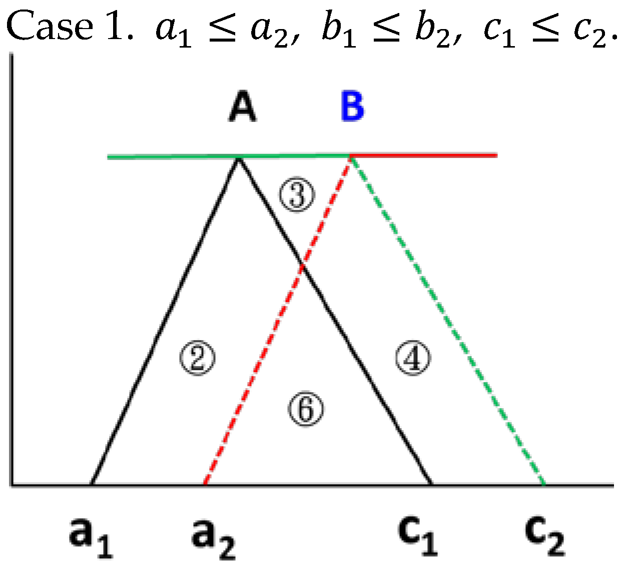
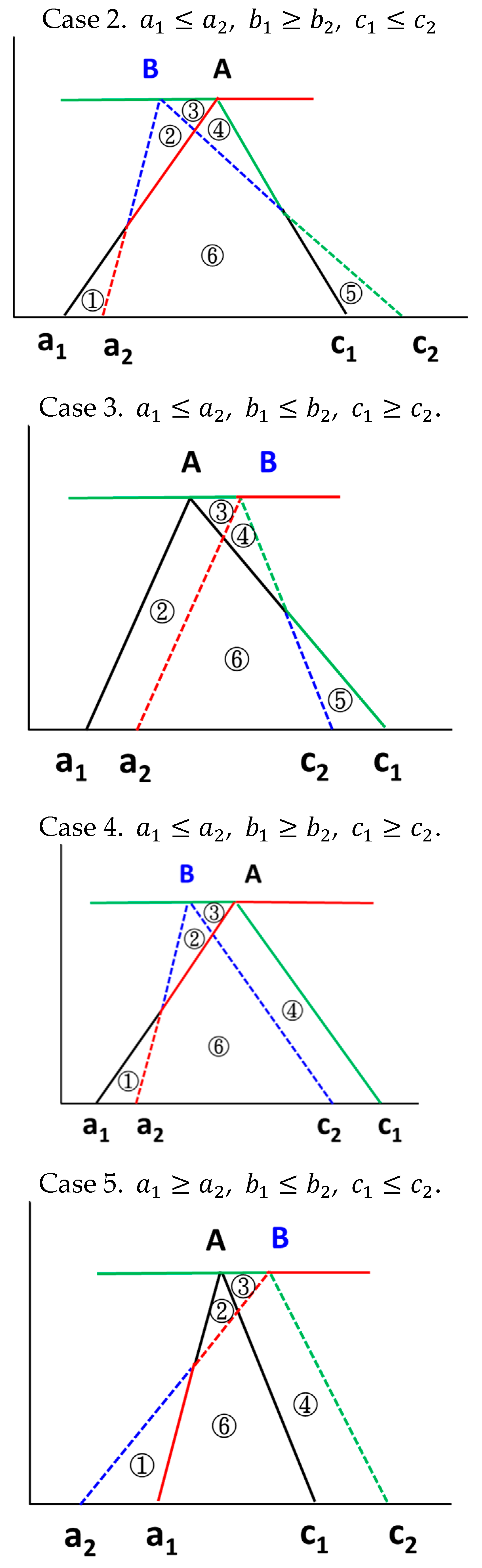
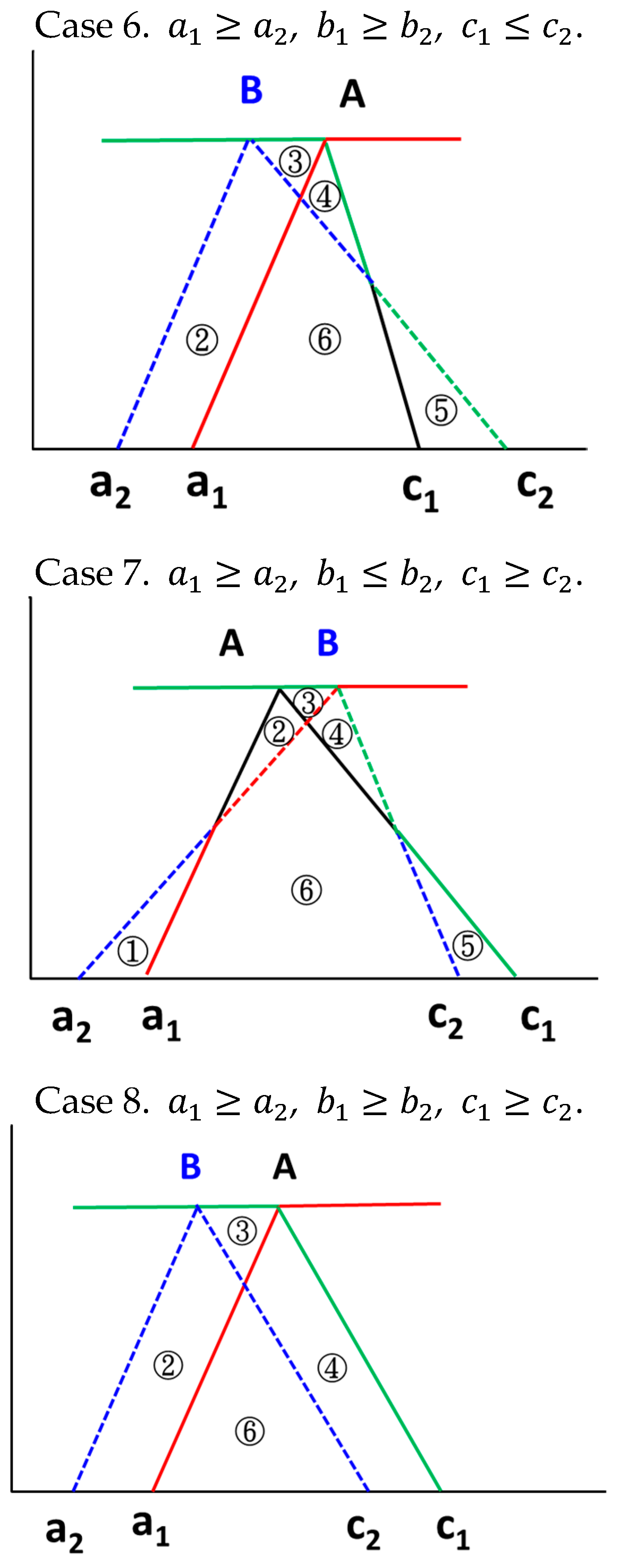
Let $A\left(a_1,b_1,c_1\right)$ and $B\left(a_2,b_2,c_2\right)$ be two triangular fuzzy numbers. Figure 1 displays eight test cases of representing all the possible cases the way two fuzzy numbers A and B can overlap with each other.

Table 1. The area $Q_i$ of i-th region for eight cases.

Case	Area
1	$Q_3={{\displaystyle \int }}_{\left(c_1-a_2\right)/\left(c_1-b_1+b_2-a_2\right)}^1-\left(c_1-a_2-\left(c_1-b_1+b_2-a_2\right)\alpha \right)d\alpha$ $Q_2={{\displaystyle \int }}_0^1{a}_2-a_1+\left(b_2-a_2-b_1+a_1\right)\alpha d\alpha -Q_3$ $Q_4={{\displaystyle \int }}_0^1{c}_2-c_1-\left(c_2-b_2-c_1+b_1\right)\alpha d\alpha -Q_3$ $Q_6={{\displaystyle \int }}_0^{\left(c_1-a_2\right)/\left(c_1-b_1+b_2-a_2\right)}(c_1-a_2-\left(c_1-b_1+b_2-a_2\right)\alpha d\alpha$
2	$Q_1={{\displaystyle \int }}_0^{\left(-a_2+a_1\right)/\left(b_2-a_2-b_1+a_1\right)}{a}_2-a_1+\left(b_2-a_2-b_1+a_1\right)\alpha d\alpha$ $Q_3={{\displaystyle \int }}_{\left(c_2-a_1\right)/\left(c_2-b_2+b_1-a_1\right)}^1-\left(c_2-a_1-\left(c_2-b_2+b_1-a_1\right)\alpha \right)d\alpha$ $Q_2={{\displaystyle \int }}_{(-a_1+a_2)/\left(b_1-a_1-b_2+a_2\right)}^1{a}_1-a_2+\left(b_1-a_1-b_2+a_2\right)\alpha d\alpha -Q_3$ $Q_4={{\displaystyle \int }}_{\left(c_1-c_2\right)/\left(c_1-b_1-c_2+b_2\right)}^1{c}_1-c_2-\left(c_1-b_1-c_2+b_2\right)\alpha d\alpha -Q_3$ $Q_5={{\displaystyle \int }}_0^{\left(c_2-c_1\right)/\left(c_2-b_2-c_1+b_1\right)}{c}_2-c_1-\left(c_2-b_2-c_1+b_1\right)\alpha d\alpha$ $Q_6={{\displaystyle \int }}_0^{\left(c_2-a_1\right)/\left(c_2-b_2+b_1-a_1\right)}\left(c_2-a_1-\left(c_2-b_2+b_1-a_1\right)\alpha \right)d\alpha -Q_1-Q_5$
3	$Q_3={{\displaystyle \int }}_{\left(c_1-a_2\right)/\left(c_1-b_1+b_2-a_2\right)}^1-\left(c_1-a_2-\left(c_1-b_1+b_2-a_2\right)\alpha \right)d\alpha$ $Q_2={{\displaystyle \int }}_0^1{a}_2-a_1+\left(b_2-a_2-b_1+a_1\right)\alpha d\alpha -Q_3$ $Q_4={{\displaystyle \int }}_{\left(c_2-c_1\right)/\left(c_2-b_2-c_1+b_1\right)}^1{c}_2-c_1-\left(c_2-b_2-c_1+b_1\right)\alpha d\alpha -Q_3$ $Q_5={{\displaystyle \int }}_0^{\left(c_1-c_2\right)/\left(c_1-b_1-c_2+b_2\right)}{c}_1-c_2-\left(c_1-b_1-c_2+b_2\right)\alpha d\alpha$ $Q_6={{\displaystyle \int }}_0^{\left(c_1-a_2\right)/\left(c_1-b_1+b_2-a_2\right)}(c_1-a_2-\left(c_1-b_1+b_2-a_2\right)\alpha d\alpha -Q_5$
4	$Q_1={{\displaystyle \int }}_0^{\left(-a_2+a_1\right)/\left(b_2-a_2-b_1+a_1\right)}{a}_2-a_1+\left(b_2-a_2-b_1+a_1\right)\alpha d\alpha$ $Q_3={{\displaystyle \int }}_{\left(c_2-a_1\right)/\left(c_2-b_2+b_1-a_1\right)}^1-\left(c_2-a_1-\left(c_2-b_2+b_1-a_1\right)\alpha \right)d\alpha$ $Q_2={{\displaystyle \int }}_{(-a_1+a_2)/\left(b_1-a_1-b_2+a_2\right)}^1{a}_1-a_2+\left(b_1-a_1-b_2+a_2\right)\alpha d\alpha -Q_3$ $Q_4={{\displaystyle \int }}_0^1{c}_1-c_2-\left(c_1-b_1-c_2+b_2\right)\alpha d\alpha -Q_3$ $Q_6={{\displaystyle \int }}_0^{\left(c_2-a_1\right)/\left(c_2-b_2+b_1-a_1\right)}\left(c_2-a_1-\left(c_2-b_2+b_1-a_1\right)\alpha \right)d\alpha -Q_1$
5	$Q_1={{\displaystyle \int }}_0^{(-a_1+a_2)/\left(b_1-a_1-b_2+a_2\right)}{a}_1-a_2+\left(b_1-a_1-b_2+a_2\right)\alpha d\alpha$ $Q_3={{\displaystyle \int }}_{\left(c_1-a_2\right)/\left(c_1-b_1+b_2-a_2\right)}^1-\left(c_1-a_2-\left(c_1-b_1+b_2-a_2\right)\alpha \right)d\alpha$ $Q_2={{\displaystyle \int }}_{\left(-a_2+a_1\right)/\left(b_2-a_2-b_1+a_1\right)}^1{a}_2-a_1+\left(b_2-a_2-b_1+a_1\right)\alpha d\alpha -Q_3$ $Q_4={{\displaystyle \int }}_0^1{c}_2-c_1-\left(c_2-b_2-c_1+b_1\right)\alpha d\alpha -Q_3$ $Q_6={{\displaystyle \int }}_0^{\left(c_1-a_2\right)/\left(c_1-b_1+b_2-a_2\right)}(c_1-a_2-\left(c_1-b_1+b_2-a_2\right)\alpha d\alpha -Q_1$
6	$Q_3={{\displaystyle \int }}_{\left(c_2-a_1\right)/\left(c_2-b_2+b_1-a_1\right)}^1-\left(c_2-a_1-\left(c_2-b_2+b_1-a_1\right)\alpha \right)d\alpha$ $Q_2={{\displaystyle \int }}_0^1{a}_1-a_2+\left(b_1-a_1-b_2+a_2\right)\alpha d\alpha -Q_3$ $Q_4={{\displaystyle \int }}_{\left(c_1-c_2\right)/\left(c_1-b_1-c_2+b_2\right)}^1{c}_1-c_2-\left(c_1-b_1-c_2+b_2\right)\alpha d\alpha -Q_3$ $Q_5={{\displaystyle \int }}_0^{\left(c_2-c_1\right)/\left(c_2-b_2-c_1+b_1\right)}{c}_2-c_1-\left(c_2-b_2-c_1+b_1\right)\alpha d\alpha$ $Q_6={{\displaystyle \int }}_0^{\left(c_2-a_1\right)/\left(c_2-b_2+b_1-a_1\right)}\left(c_2-a_1-\left(c_2-b_2+b_1-a_1\right)\alpha \right)d\alpha -Q_5$
7	$Q_1={{\displaystyle \int }}_0^{(-a_1+a_2)/\left(b_1-a_1-b_2+a_2\right)}{a}_1-a_2+\left(b_1-a_1-b_2+a_2\right)\alpha d\alpha$ $Q_3={{\displaystyle \int }}_{\left(c_1-a_2\right)/\left(c_1-b_1+b_2-a_2\right)}^1-\left(c_1-a_2-\left(c_1-b_1+b_2-a_2\right)\alpha \right)d\alpha$ $Q_2={{\displaystyle \int }}_{\left(-a_2+a_1\right)/\left(b_2-a_2-b_1+a_1\right)}^1{a}_2-a_1+\left(b_2-a_2-b_1+a_1\right)\alpha d\alpha -Q_3$ $Q_4={{\displaystyle \int }}_{\left(c_2-c_1\right)/\left(c_2-b_2-c_1+b_1\right)}^1{c}_2-c_1-\left(c_2-b_2-c_1+b_1\right)\alpha d\alpha -Q_3$ $Q_5={{\displaystyle \int }}_0^{\left(c_1-c_2\right)/\left(c_1-b_1-c_2+b_2\right)}{c}_1-c_2-\left(c_1-b_1-c_2+b_2\right)\alpha d\alpha$ $Q_6={{\displaystyle \int }}_0^{\left(c_1-a_2\right)/\left(c_1-b_1+b_2-a_2\right)}(c_1-a_2-\left(c_1-b_1+b_2-a_2\right)\alpha d\alpha -Q_1-Q_5$
8	$Q_3={{\displaystyle \int }}_{\left(c_2-a_1\right)/\left(c_2-b_2+b_1-a_1\right)}^1-\left(c_2-a_1-\left(c_2-b_2+b_1-a_1\right)\alpha \right)d\alpha$ $Q_2={{\displaystyle \int }}_0^1{a}_1-a_2+\left(b_1-a_1-b_2+a_2\right)\alpha d\alpha -Q_3$ $Q_4={{\displaystyle \int }}_0^1{c}_1-c_2-\left(c_1-b_1-c_2+b_2\right)\alpha d\alpha -Q_3$ $Q_6={{\displaystyle \int }}_0^{\left(c_2-a_1\right)/\left(c_2-b_2+b_1-a_1\right)}\left(c_2-a_1-\left(c_2-b_2+b_1-a_1\right)\alpha \right)d\alpha$

shows the area $Q_i$ of i-th region in each case. More precisely, the eight extensive test cases are as follows:

Case 1.

$a_1\le a_2$, $b_1\le b_2$, $c_1\le c_2.$

Case 2.

$a_1\le a_2$, $b_1\ge b_2$, $c_1\le c_2.$

Case 3.

$a_1\le a_2$, $b_1\le b_2$, $c_1\ge c_2.$

Case 4.

$a_1\le a_2$, $b_1\ge b_2$, $c_1\ge c_2.$

Case 5.

$a_1\ge a_2$, $b_1\le b_2$, $c_1\le c_2.$

Case 6.

$a_1\ge a_2$, $b_1\ge b_2$, $c_1\le c_2.$

Case 7.

$a_1\ge a_2$, $b_1\le b_2$, $c_1\ge c_2.$

Case 8.

$a_1\ge a_2$, $b_1\ge b_2$, $c_1\ge c_2$.

3. Nakamura’s Fuzzy Preference Relation

Using fuzzy minimum, fuzzy maximum, and Hamming distance, Nakamura’s fuzzy preference relations [4] are defined as follows:

Definition 8.

For two fuzzy numbers A and B, Nakamura [4] defines $N\left(A,B\right)$ and $N\prime \left(A,B\right)$ as fuzzy preference relations by the following membership functions:

$$N\left(A,B\right)=\frac{d\left(\underset{¯}{A},\widetilde{min}\left(\underset{¯}{A},\underset{¯}{B}\right)\right)+d\left(\overline{A},\widetilde{min}\left(\overline{A},\overline{B}\right)\right)}{d\left(\underset{¯}{A},\underset{¯}{B}\right)+d\left(\overline{A},\overline{B}\right)}$$

and:

$$N\prime \left(A,B\right)=\frac{d\left(A{{\displaystyle \cap }}^{}B,0\right)+d\left(\mathrm{A},\widetilde{max}\left(A,\mathrm{B}\right)\right)}{d\left(A,0\right)+d\left(B,0\right)}$$

respectively. Yuan [6] showed that N$\left(A,B\right)$ is reciprocal and transitive, but not robust. Wang and Kerre [3] derived that:

$$\begin{gathered} d\left(\underset{¯}{A},\widetilde{min}\left(\underset{¯}{A},\underset{¯}{B}\right)\right)=d\left(\underset{¯}{B},\widetilde{max}\left(\underset{¯}{A},\underset{¯}{B}\right)\right) \\ d\left(\overline{A},\widetilde{max}\left(\overline{A},\overline{B}\right)\right)=d\left(\overline{B},\widetilde{min}\left(\overline{A},\overline{B}\right)\right) \\ d\left(\underset{¯}{A},\widetilde{min}\left(\underset{¯}{A},\underset{¯}{B}\right)\right)+d\left(\underset{¯}{A},\widetilde{max}\left(\underset{¯}{A},\underset{¯}{B}\right)\right)=d\left(\underset{¯}{A},\underset{¯}{B}\right) \\ d\left(\overline{A},\widetilde{min}\left(\overline{A},\overline{B}\right)\right)+d\left(\overline{A},\widetilde{max}\left(\overline{A},\overline{B}\right)\right)=d\left(\overline{A},\overline{B}\right) \end{gathered}$$

and:

$$2d\left(\mathrm{A}{{\displaystyle \cap }}^{}\mathrm{B},0\right)+d\left(\mathrm{A},\widetilde{max}\left(A,\mathrm{B}\right)\right)+d\left(\mathrm{B},\widetilde{max}\left(A,\mathrm{B}\right)\right)=d\left(A,0\right)+d\left(B,0\right).$$

It follows that:

$$N\left(A,B\right)+N\left(B,A\right)=1$$

and:

$$N\prime \left(A,B\right)+N\prime \left(B,A\right)=1.$$

For two triangular fuzzy numbers $A\left(a_1,b_1,c_1\right)$ and $B\left(a_2,b_2,c_2\right)$, then:

$$\begin{gathered} A_{\alpha }=\left[L_1,U_1\right]=\left[a_1+\left(b_1-a_1\right)\alpha ,c_1-\left(c_1-b_1\right)\alpha \right] \\ {B}_{\alpha }=\left[L_2,U_2\right]=\left[a_2+\left(b_2-a_2\right)\alpha ,c_2-\left(c_2-b_2\right)\alpha \right] \end{gathered}$$

so:

$$\begin{gathered} N\left(A,B\right)=\frac{d\left(\underset{¯}{A},\widetilde{min}\left(\underset{¯}{A},\underset{¯}{B}\right)\right)+d\left(\overline{A},\widetilde{min}\left(\overline{A},\overline{B}\right)\right)}{d\left(\underset{¯}{A},\underset{¯}{B}\right)+d\left(\overline{A},\overline{B}\right)} \\ =\frac{{{\displaystyle \int }}_{L_1\ge L_2}{L}_1-L_{2}d\alpha +{{\displaystyle \int }}_{U_1\ge U_2}{U}_1-U_{2}d\alpha }{{{\displaystyle \int }}_{L_1\ge L_2}{L}_1-L_{2}d\alpha +{{\displaystyle \int }}_{L_2\ge L_1}{L}_2-L_{1}d\alpha +{{\displaystyle \int }}_{U_1\ge U_2}{U}_1-U_{2}d\alpha +{{\displaystyle \int }}_{U_2\ge U_1}{U}_2-U_{1}d\alpha }. \end{gathered}$$

Define:

$$\begin{gathered} S_1={{\displaystyle \int }}_{L_1\ge L_2}{L}_1-L_{2}d\alpha ={{\displaystyle \int }}_{a_1-a_2+\left(b_1-a_1-b_2+a_2\right)\alpha \ge 0}{a}_1-a_2+\left(b_1-a_1-b_2+a_2\right)\alpha d\alpha \\ {S}_2={{\displaystyle \int }}_{L_2\ge L_1}{L}_2-L_{1}d\alpha ={{\displaystyle \int }}_{a_2-a_1+\left(b_2-a_2-b_1+a_1\right)\alpha \ge 0}{a}_2-a_1+\left(b_2-a_2-b_1+a_1\right)\alpha d\alpha \\ {S}_3={{\displaystyle \int }}_{U_1\ge U_2}{U}_1-U_{2}d\alpha ={{\displaystyle \int }}_{c_1-c_2-\left(c_1-b_1-c_2+b_2\right)\alpha \ge 0}{c}_1-c_2-\left(c_1-b_1-c_2+b_2\right)\alpha d\alpha \\ {S}_4={{\displaystyle \int }}_{U_2\ge U_1}{U}_2-U_{1}d\alpha ={{\displaystyle \int }}_{c_2-c_1-\left(c_2-b_2-c_1+b_1\right)\alpha \ge 0}{c}_2-c_1-\left(c_2-b_2-c_1+b_1\right)\alpha d\alpha , \end{gathered}$$

then:

$$N\left(A,B\right)=\frac{S_1+S_3}{S_1+S_2+S_3+S_4}.$$

Let $\mathcal{A}=a_2-a_1$, $ℬ=b_2-b_1$ and $\mathcal{C}=c_2-c_1$. The steps for implementing the Nakamura’s fuzzy preference relation $N\left(A,B\right)$ are as in Algorithm 1:

Algorithm 1. Nakamura’s fuzzy preference relation

If $\mathcal{A}\ge 0$

If $\mathcal{C}\ge 0$

If $ℬ\ge 0$, then $N\left(A,B\right)=0$ else $N\left(A,B\right)=\frac{{ℬ}^2\left(\mathcal{A}-2ℬ+\mathcal{C}\right)}{\left({\mathcal{A}}^2+{ℬ}^2\right)\left(-ℬ+\mathcal{C}\right)+\left({ℬ}^2+{\mathcal{C}}^2\right)\left(\mathcal{A}-ℬ\right)}$.

else if $ℬ\ge 0$, then $N\left(A,B\right)=\frac{{\mathcal{C}}^2}{\left(\mathcal{A}+ℬ\right)\left(ℬ-\mathcal{C}\right)+{ℬ}^2+{\mathcal{C}}^2}$ else

$N\left(A,B\right)=1-\frac{{\mathcal{A}}^2}{\left(\mathcal{A}-ℬ\right)\left(-ℬ-\mathcal{C}\right)+{\mathcal{A}}^2+{ℬ}^2}$.

else if $\mathcal{C}\ge 0$

If $ℬ\ge 0$, then $N\left(A,B\right)=\frac{{\mathcal{A}}^2}{\left(-\mathcal{A}+ℬ\right)\left(ℬ+\mathcal{C}\right)+{\mathcal{A}}^2+{ℬ}^2}$ else

$N\left(A,B\right)=1-\frac{{\mathcal{C}}^2}{\left(\mathcal{A}+ℬ\right)\left(ℬ-\mathcal{C}\right)+{ℬ}^2+{\mathcal{C}}^2}$.

else if $ℬ\ge 0$, then $N\left(A,B\right)=1-\frac{{ℬ}^2\left(\mathcal{A}-2ℬ+\mathcal{C}\right)}{\left({\mathcal{A}}^2+{ℬ}^2\right)\left(-ℬ+\mathcal{C}\right)+\left({ℬ}^2+{\mathcal{C}}^2\right)\left(\mathcal{A}-ℬ\right)}$ else $N\left(A,B\right)=1$.

Table 2. $N\left(A,B\right)$ and $N\prime \left(A,B\right)$ for eight cases.

Case	$\mathit{N}\left(\mathit{A},\mathit{B}\right)$	${\mathit{N}}^{\prime }\left(\mathit{A},\mathit{B}\right)$
1	0	$1+\frac{{\left(a_2-c_1\right)}^2}{\left(a_2+b_1-b_2-c_1\right)\left(-a_1-a_2+c_1+c_2\right)}$
2	$\frac{{\left(b_2-b_1\right)}^2\left(a_2-a_1-2\left(b_2-b_1\right)+\left(c_2-c_1\right)\right)}{\left({\left(a_2-a_1\right)}^2+{\left(b_2-b_1\right)}^2\right)\left(b_1-b_2+c_2-c_1\right)+\left({\left(b_2-b_1\right)}^2+{\left(c_2-c_1\right)}^2\right)\left(a_2-a_1-b_2+b_1\right)}$	$\frac{{\left(a_1-c_2\right)}^2}{\left(a_1-b_1+b_2-c_2\right)\left(a_1+a_2-c_1-c_2\right)}$
3	$\frac{{\left(c_2-c_1\right)}^2}{\left(a_2-a_1+b_2-b_1\right)\left(b_2-b_1-c_2+c_1\right)+{\left(b_2-b_1\right)}^2+{\left(c_2-c_1\right)}^2}$	$1+\frac{{\left(a_2-c_1\right)}^2}{\left(a_2+b_1-b_2-c_1\right)\left(-a_1-a_2+c_1+c_2\right)}$
4	$1-\frac{{\left(a_2-a_1\right)}^2}{\left(a_2-a_1-b_2+b_1\right)\left(-b_2+b_1-c_2+c_1\right)+{\left(a_2-a_1\right)}^2+{\left(b_2-b_1\right)}^2}$	$\frac{{\left(a_1-c_2\right)}^2}{\left(a_1-b_1+b_2-c_2\right)\left(a_1+a_2-c_1-c_2\right)}$
5	$\frac{{\left(a_2-a_1\right)}^2}{\left(a_2-a_1-b_2+b_1\right)\left(-b_2+b_1-c_2+c_1\right)+{\left(a_2-a_1\right)}^2+{\left(b_2-b_1\right)}^2}$	$1+\frac{{\left(a_2-c_1\right)}^2}{\left(a_2+b_1-b_2-c_1\right)\left(-a_1-a_2+c_1+c_2\right)}$
6	$1-\frac{{\left(c_2-c_1\right)}^2}{\left(a_2-a_1+b_2-b_1\right)\left(b_2-b_1-c_2+c_1\right)+{\left(b_2-b_1\right)}^2+{\left(c_2-c_1\right)}^2}$	$\frac{{\left(a_1-c_2\right)}^2}{\left(a_1-b_1+b_2-c_2\right)\left(a_1+a_2-c_1-c_2\right)}$
7	$1-\frac{{\left(b_2-b_1\right)}^2\left(a_2-a_1-2b_2+2b_1+c_2-c_1\right)}{\left({\left(a_2-a_1\right)}^2+{\left(b_2-b_1\right)}^2\right)\left(b_1-b_2+c_2-c_1\right)+\left({\left(b_2-b_1\right)}^2+{\left(c_2-c_1\right)}^2\right)\left(a_2-a_1-b_2+b_1\right)}$	$1+\frac{{\left(a_2-c_1\right)}^2}{\left(a_2+b_1-b_2-c_1\right)\left(-a_1-a_2+c_1+c_2\right)}$
8	1	$\frac{{\left(a_1-c_2\right)}^2}{\left(a_1-b_1+b_2-c_2\right)\left(a_1+a_2-c_1-c_2\right)}$

shows the values of $N\left(A,B\right)$ and $N\prime \left(A,B\right)$ for each test case. The first observation of this table is that:

$$\begin{gathered} N_1\left(A,B\right)+N_8\left(A,B\right)=1 \\ {N}_2\left(A,B\right)+N_7\left(A,B\right)=1 \\ {N}_3\left(A,B\right)+N_6\left(A,B\right)=1 \\ {N}_4\left(A,B\right)+N_5\left(A,B\right)=1. \end{gathered}$$

Secondly, comparing the values of $N\left(A,B\right)$ with that of $N\prime \left(A,B\right)$, we have that $1-N_1^{\prime }\left(A,B\right)\ge N_1\left(A,B\right)$ and $1-N_8^{\prime }\left(A,B\right)\le N_8\left(A,B\right)$. If $a_2+2b_2+c_2\ge a_1-2b_1-c_1$, we obtain that $1-N_2^{\prime }\left(A,B\right)\le N_2\left(A,B\right)$, $1-N_3^{\prime }\left(A,B\right)\ge N_3\left(A,B\right)$, $1-N_4^{\prime }\left(A,B\right)\le N_4\left(A,B\right)$, $1-N_5^{\prime }\left(A,B\right)\ge N_5\left(A,B\right)$, $1-N_6^{\prime }\left(A,B\right)\le N_6\left(A,B\right)$ and $1-N_7^{\prime }\left(A,B\right)\ge N_7\left(A,B\right)$.

4. Kołodziejczyk’s Fuzzy Preference Relation

By considering the common part of two membership functions, Kołodziejczyk’s method [5] is based on fuzzy maximum and Hamming distance to propose the following fuzzy preference relations:

Definition 9.

For two fuzzy numbers A and B, Kołodziejczyk [5] defines $K1\prime \left(A,B\right)$ and $K2\prime \left(A,B\right)$ as fuzzy preference relations by the following membership functions:

$$K1\prime \left(A,B\right)=\frac{d\left(\underset{¯}{A},\widetilde{max}\left(\underset{¯}{A},\underset{¯}{B}\right)\right)+d\left(\overline{A},\widetilde{max}\left(\overline{A},\overline{B}\right)\right)+d\left(A{{\displaystyle \cap }}^{}B,0\right)}{d\left(\underset{¯}{A},\underset{¯}{B}\right)+d\left(\overline{A},\overline{B}\right)+2d\left(A{{\displaystyle \cap }}^{}B,0\right)}$$

and:

$$K2\prime \left(A,B\right)=\frac{d\left(\underset{¯}{A},\tilde{\max }\left(\underset{¯}{A},\underset{¯}{B}\right)\right)+d\left(\overline{A},\tilde{\max }\left(\overline{A},\overline{B}\right)\right)}{d\left(\underset{¯}{A},\underset{¯}{B}\right)+d\left(\overline{A},\overline{B}\right)}$$

respectively. $K1\prime \left(A,B\right)$ is reciprocal, transitive and robust [3,5]. Since:

$$K2\prime \left(A,B\right)=1-N\left(A,B\right)$$

the results of $K2\prime \left(A,B\right)$ can be obtained from those of $N\left(A,B\right)$.

For two triangular fuzzy numbers $A\left(a_1,b_1,c_1\right)$ and $B\left(a_2,b_2,c_2\right)$, then:

$$\begin{gathered} A_{\alpha }=\left[L_1,U_1\right]=\left[a_1+\left(b_1-a_1\right)\alpha ,c_1-\left(c_1-b_1\right)\alpha \right] \\ {B}_{\alpha }=\left[L_2,U_2\right]=\left[a_2+\left(b_2-a_2\right)\alpha ,c_2-\left(c_2-b_2\right)\alpha \right]. \end{gathered}$$

Define:

$$\begin{gathered} S_1=d\left(\underset{¯}{A},\widetilde{max}\left(\underset{¯}{A},\underset{¯}{B}\right)\right)={{\displaystyle \int }}_{L_2\ge L_1}{L}_2-L_{1}d\alpha \\ {S}_2={{\displaystyle \int }}_{L_1\ge L_2}{L}_1-L_{2}d\alpha \\ d\left(\underset{¯}{A},\underset{¯}{B}\right)=S_1+S_2 \\ {S}_3=d\left(\overline{A},\widetilde{max}\left(\overline{A},\overline{B}\right)\right)={{\displaystyle \int }}_{U_2\ge U_1}{U}_2-U_{1}d\alpha \\ {S}_4={{\displaystyle \int }}_{U_1\ge U_2}{U}_1-U_{2}d\alpha \\ d\left(\overline{A},\overline{B}\right)=S_3+S_4 \end{gathered}$$

and:

$$S_5=d\left(A{{\displaystyle \cap }}^{}B,0\right)={{\displaystyle \int }}_{U_1\ge L_2}{U}_1-L_{2}d\alpha -{{\displaystyle \int }}_{U_1\ge U_2}{U}_1-U_{2}d\alpha -{{\displaystyle \int }}_{L_1\ge L_2}{L}_1-L_{2}d\alpha .$$

Then:

$$K1\prime \left(A,B\right)=\frac{S_1+S_3+S_5}{S_1+S_2+S_3+S_4+2S_5}$$

and:

$$K2\prime \left(A,B\right)=\frac{S_1+S_3}{S_1+S_2+S_3+S_4}.$$

In

Table 3. $K1\prime \left(A,B\right)$ and $K2\prime \left(A,B\right)$ for eight cases.

Case	$\mathit{K}{1}^{\prime }\left(\mathit{A},\mathit{B}\right)$	$\mathit{K}{2}^{\prime }\left(\mathit{A},\mathit{B}\right)$
1	$1-\frac{{\left(c_1-a_2\right)}^2}{\left(c_1-a_2+c_2-a_1\right)\left(c_1-a_2-b_1+b_2\right)+2{\left(b_2-b_1\right)}^2}$	1
2	$\frac{{\left(c_2-a_1\right)}^2}{{\left(c_2-a_1\right)}^2+\left(c_2-a_1-b_2+b_1\right)\left(c_1-a_2-b_2+b_1\right)+{\left(b_2-b_1\right)}^2}$	$1-\frac{{\left(b_2-b_1\right)}^2\left(a_2-a_1-2\left(b_2-b_1\right)+\left(c_2-c_1\right)\right)}{\left({\left(a_2-a_1\right)}^2+{\left(b_2-b_1\right)}^2\right)\left(b_1-b_2+c_2-c_1\right)+\left({\left(b_2-b_1\right)}^2+{\left(c_2-c_1\right)}^2\right)\left(a_2-a_1-b_2+b_1\right)}$
3	$1-\frac{{\left(c_1-a_2\right)}^2}{\left(c_1-a_2+c_2-a_1\right)\left(c_1-a_2-b_1+b_2\right)+2{\left(b_2-b_1\right)}^2}$	$1-\frac{{\left(c_2-c_1\right)}^2}{\left(a_2-a_1+b_2-b_1\right)\left(b_2-b_1-c_2+c_1\right)+{\left(b_2-b_1\right)}^2+{\left(c_2-c_1\right)}^2}$
4	$\frac{{\left(c_2-a_1\right)}^2}{{\left(c_2-a_1\right)}^2+\left(c_2-a_1-b_2+b_1\right)\left(c_1-a_2-b_2+b_1\right)+{\left(b_2-b_1\right)}^2}$	$\frac{{\left(a_2-a_1\right)}^2}{\left(a_2-a_1-b_2+b_1\right)\left(-b_2+b_1-c_2+c_1\right)+{\left(a_2-a_1\right)}^2+{\left(b_2-b_1\right)}^2}$
5	$1-\frac{{\left(c_1-a_2\right)}^2}{\left(c_1-a_2+c_2-a_1\right)\left(c_1-a_2-b_1+b_2\right)+2{\left(b_2-b_1\right)}^2}$	$1-\frac{{\left(a_2-a_1\right)}^2}{\left(a_2-a_1-b_2+b_1\right)\left(-b_2+b_1-c_2+c_1\right)+{\left(a_2-a_1\right)}^2+{\left(b_2-b_1\right)}^2}$
6	$\frac{{\left(c_2-a_1\right)}^2}{{\left(c_2-a_1\right)}^2+\left(c_2-a_1-b_2+b_1\right)\left(c_1-a_2-b_2+b_1\right)+{\left(b_2-b_1\right)}^2}$	$\frac{{\left(c_2-c_1\right)}^2}{\left(a_2-a_1+b_2-b_1\right)\left(b_2-b_1-c_2+c_1\right)+{\left(b_2-b_1\right)}^2+{\left(c_2-c_1\right)}^2}$
7	$1-\frac{{\left(c_1-a_2\right)}^2}{\left(c_1-a_2+c_2-a_1\right)\left(c_1-a_2-b_1+b_2\right)+2{\left(b_2-b_1\right)}^2}$	$\frac{{\left(b_2-b_1\right)}^2\left(a_2-a_1-2b_2+2b_1+c_2-c_1\right)}{\left({\left(a_2-a_1\right)}^2+{\left(b_2-b_1\right)}^2\right)\left(b_1-b_2+c_2-c_1\right)+\left({\left(b_2-b_1\right)}^2+{\left(c_2-c_1\right)}^2\right)\left(a_2-a_1-b_2+b_1\right)}$
8	$\frac{{\left(c_2-a_1\right)}^2}{{\left(c_2-a_1\right)}^2+\left(c_2-a_1-b_2+b_1\right)\left(c_1-a_2-b_2+b_1\right)+{\left(b_2-b_1\right)}^2}$	0

, we display the values of $K1\prime \left(A,B\right)$ and $K2\prime \left(A,B\right)$ for each test case. An examination of the table reveals that:

$$\begin{gathered} K{1}_1^{\prime }\left(A,B\right)=K{1}_3^{\prime }\left(A,B\right)=K{1}_5^{\prime }\left(A,B\right)=K{1}_7^{\prime }\left(A,B\right) \\ =1-\frac{{\left(c_1-a_2\right)}^2}{\left(c_1-a_2+c_2-a_1\right)\left(c_1-a_2-b_1+b_2\right)+2{\left(b_2-b_1\right)}^2} \end{gathered}$$

and:

$$K{1}_2^{\prime }\left(A,B\right)=K{1}_4^{\prime }\left(A,B\right)=K{1}_6^{\prime }\left(A,B\right)=K{1}_8^{\prime }\left(A,B\right)=\frac{{\left(c_2-a_1\right)}^2}{{\left(c_2-a_1\right)}^2+\left(c_2-a_1-b_2+b_1\right)\left(c_1-a_2-b_2+b_1\right)+{\left(b_2-b_1\right)}^2}.$$

If $b_1=b_2$, we have:

$$K{1}_1^{\prime }\left(A,B\right)=1-\frac{c_1-a_2}{\left(c_1-a_2+c_2-a_1\right)}=\frac{c_2-a_1}{\left(c_1-a_2+c_2-a_1\right)}$$

and:

$$K{1}_2^{\prime }\left(A,B\right)=\frac{c_2-a_1}{\left(c_1-a_2+c_2-a_1\right)}$$

so:

$$K{1}_1^{\prime }\left(A,B\right)=K{1}_2^{\prime }\left(A,B\right)$$

and:

$$K{1}_1^{\prime }\left(A,B\right)+K{1}_2^{\prime }\left(A,B\right)=\frac{2\left(c_2-a_1\right)}{\left(c_1-a_2+c_2-a_1\right)}.$$

It follows that:

$$K{1}_1^{\prime }\left(A,B\right)+K{1}_2^{\prime }\left(A,B\right)=0\mathrm{for}{b}_1=b_2\mathrm{and}{c}_2=a_1.$$

and:

$$K{1}_1^{\prime }\left(A,B\right)+K{1}_2^{\prime }\left(A,B\right)=1\mathrm{for}{b}_1=b_2\mathrm{and}{c}_1-a_2=c_2-a_1.$$

5. Two Comparative Studies of Decomposition and Intersection of Two Fuzzy Numbers

If the fuzzy number A is less than the fuzzy number B, then the Hamming distance between A and $\widetilde{max}\left(A,B\right)$ is large. Two representations are adopted. One is $\mathrm{d}\left(A,\widetilde{max}\left(A,B\right)\right)$. The other is $d\left(\underset{¯}{A},\widetilde{max}\left(\underset{¯}{A},\underset{¯}{B}\right)\right)+d\left(\overline{A},\widetilde{max}\left(\overline{A},\overline{B}\right)\right)$ which decomposes A into $\overline{A}$ and $\underset{¯}{A}$. To analyze the effect of decomposition, we consider the following preference relations without decomposition:

$$T1\prime \left(A,B\right)=\frac{d\left(A,\tilde{\max }\left(A,B\right)\right)+d\left(A{{\displaystyle \cap }}^{}B,0\right)}{d\left(A,0\right)+d\left(B,0\right)}$$

and:

$$T2\prime \left(A,B\right)=\frac{d\left(A,\tilde{\max }\left(A,B\right)\right)}{d\left(A,B\right)}$$

which are the counterparts of the Kołodziejczyk’s preference relations $K1\prime \left(A,B\right)$ and $K2\prime \left(A,B\right)$. Therefore, the preference relations $K1\prime \left(A,B\right)$ and $K2\prime \left(A,B\right)$ consider the decomposition of fuzzy numbers, while $T1\prime \left(A,B\right)$ and $T2\prime \left(A,B\right)$ do not. The preference relations $K1\prime \left(A,B\right)$ and $T1\prime \left(A,B\right)$ consider the intersection of two membership functions, while $K2\prime \left(A,B\right)$ and $T2\prime \left(A,B\right)$ do not. For completeness,

Table 4. $N\left(A,B\right)$ , $N\prime \left(A,B\right)$, $K1\prime \left(A,B\right)$, $K2\prime \left(A,B\right)$, $T1\prime \left(A,B\right)$ and $T2\prime \left(A,B\right)$ for eight cases.

Case	$\mathit{N}\left(\mathit{A},\mathit{B}\right)$	${\mathit{N}}^{\prime }\left(\mathit{A},\mathit{B}\right)$	$\mathit{K}{1}^{\prime }\left(\mathit{A},\mathit{B}\right)$	$\mathit{K}{2}^{\prime }\left(\mathit{A},\mathit{B}\right)$	$\mathit{T}{1}^{\prime }\left(\mathit{A},\mathit{B}\right)$	$\mathit{T}{2}^{\prime }\left(\mathit{A},\mathit{B}\right)$
1	0	$\frac{Q_2+Q_4+Q_6}{Q_2+Q_4+2Q_6}$	$\frac{Q_2+2Q_3+Q_4+Q_6}{Q_2+2Q_3+Q_4+2Q_6}$	1	$\frac{Q_2+Q_4+Q_6}{Q_2+Q_4+2Q_6}$	1
2	$\frac{Q_2+2Q_3+Q_4}{Q_1+Q_2+2Q_3+Q_4+Q_5}$	$\frac{Q_1+Q_5+Q_6}{Q_1+Q_2+Q_4+Q_5+2Q_6}$	$\frac{Q_1+Q_5+Q_6}{Q_1+Q_2+2Q_3+Q_4+Q_5+2Q_6}$	$\frac{Q_1+Q_5}{Q_1+Q_2+2Q_3+Q_4+Q_5}$	$\frac{Q_1+Q_5+Q_6}{Q_1+Q_2+Q_4+Q_5+2Q_6}$	$\frac{Q_1+Q_5}{Q_1+Q_2+Q_4+Q_5}$
3	$\frac{Q_5}{Q_2+2Q_3+Q_4+Q_5}$	$\frac{Q_2+Q_4+Q_6}{Q_2+Q_4+Q_5+2Q_6}$	$\frac{Q_2+2Q_3+Q_4+Q_6}{Q_2+2Q_3+Q_4+Q_5+2Q_6}$	$\frac{Q_2+2Q_3+Q_4}{Q_2+2Q_3+Q_4+Q_5}$	$\frac{Q_2+Q_4+Q_6}{Q_2+Q_4+Q_5+2Q_6}$	$\frac{Q_2+Q_4}{Q_2+Q_4+Q_5}$
4	$\frac{Q_2+2Q_3+Q_4}{Q_1+Q_2+2Q_3+Q_4}$	$\frac{Q_1+Q_6}{Q_1+Q_2+Q_4+2Q_6}$	$\frac{Q_1+Q_6}{Q_1+Q_2+2Q_3+Q_4+2Q_6}$	$\frac{Q_1}{Q_1+Q_2+2Q_3+Q_4}$	$\frac{Q_1+Q_6}{Q_1+Q_2+Q_4+2Q_6}$	$\frac{Q_1}{Q_1+Q_2+Q_4}$
5	$\frac{Q_1}{Q_1+Q_2+2Q_3+Q_4}$	$\frac{Q_2+Q_4+Q_6}{Q_1+Q_2+Q_4+2Q_6}$	$\frac{Q_2+2Q_3+Q_4+Q_6}{Q_1+Q_2+2Q_3+Q_4+2Q_6}$	$\frac{Q_2+2Q_3+Q_4}{Q_1+Q_2+2Q_3+Q_4}$	$\frac{Q_2+Q_4+Q_6}{Q_1+Q_2+Q_4+2Q_6}$	$\frac{Q_2+Q_4}{Q_1+Q_2+Q_4}$
6	$\frac{Q_2+2Q_3+Q_4}{Q_2+2Q_3+Q_4+Q_5}$	$\frac{Q_5+Q_6}{Q_2+Q_4+Q_5+2Q_6}$	$\frac{Q_5+Q_6}{Q_2+2Q_3+Q_4+Q_5+2Q_6}$	$\frac{Q_5}{Q_2+2Q_3+Q_4+Q_5}$	$\frac{Q_5+Q_6}{Q_2+Q_4+Q_5+2Q_6}$	$\frac{Q_5}{Q_2+Q_4+Q_5}$
7	$\frac{Q_1+Q_5}{Q_1+Q_2+2Q_3+Q_4+Q_5}$	$\frac{Q_2+Q_4+Q_6}{Q_1+Q_2+Q_4+Q_5+2Q_6}$	$\frac{Q_2+2Q_3+Q_4+Q_6}{Q_1+Q_2+2Q_3+Q_4+Q_5+2Q_6}$	$\frac{Q_2+2Q_3+Q_4}{Q_1+Q_2+2Q_3+Q_4+Q_5}$	$\frac{Q_2+Q_4+Q_6}{Q_1+Q_2+Q_4+Q_5+2Q_6}$	$\frac{Q_2+Q_4}{Q_1+Q_2+Q_4+Q_5}$
8	1	$\frac{Q_6}{Q_2+Q_4+2Q_6}$	$\frac{Q_6}{Q_2+2Q_3+Q_4+2Q_6}$	0	$\frac{Q_6}{Q_2+Q_4+2Q_6}$	0

displays the values of $N\left(A,B\right)$, $N\prime \left(A,B\right)$, $K1\prime \left(A,B\right)$, $K2\prime \left(A,B\right)$, $T1\prime \left(A,B\right)$ and $T2\prime \left(A,B\right)$ of each test case in terms of the values of $Q_i$. The $K1\prime \left(A,B\right)$ considers both decomposition and intersection of two fuzzy numbers, while $T2\prime \left(A,B\right)$ do not. From $K1\prime \left(A,B\right)$ to $T2\prime \left(A,B\right)$, two representations are:

$$K1\prime \left(A,B\right)\to K2\prime \left(A,B\right)\to T2\prime \left(A,B\right)$$

and:

$$K1\prime \left(A,B\right)\to T1\prime \left(A,B\right)\to T2\prime \left(A,B\right).$$

The first feature of Table 4 is that the differences between $K1\prime \left(A,B\right)$ and $T1\prime \left(A,B\right)$ and between $K2\prime \left(A,B\right)$ and $T2\prime \left(A,B\right)$ are $Q_3$. More precisely, the numerators and denominators of both $K1\prime \left(A,B\right)$ and $K2\prime \left(A,B\right)$ include $2Q_3$ for cases 1, 3, 5 and 7, the denominators of both $K1\prime \left(A,B\right)$ and $K2\prime \left(A,B\right)$ include $2Q_3$ for cases 2, 4, 6 and 8. Therefore, $2Q_3$ represents the effect of the decomposition of fuzzy numbers. The differences between $K1\prime \left(A,B\right)$ and $K2\prime \left(A,B\right)$ and between $T1\prime \left(A,B\right)$ and $T2\prime \left(A,B\right)$ are $Q_6$. More precisely, the numerators and denominators of both $K1\prime \left(A,B\right)$ and $T1\prime \left(A,B\right)$ include $Q_6$ and $2Q_6$, respectively. Therefore, $Q_6$ represents the effect of the intersection of two membership functions. After some computations, the characteristics of $K1\prime \left(A,B\right)$, $K2\prime \left(A,B\right)$, $T1\prime \left(A,B\right)$ and $T2\prime \left(A,B\right)$ are described as follows:

Theorem 1.

Let $T2\prime \left(A,B\right)=\frac{\alpha }{\alpha +\beta }$.

(1)

If $b_1\le b_2$, $\mathsf{\beta }\le 2Q_3+\alpha$ or $b_1\ge b_2$, $\mathsf{\beta }+2Q_3\le \alpha$, then $K1\prime \left(A,B\right)\le K2\prime \left(A,B\right)$. If $b_1\le b_2$, $\mathsf{\beta }\ge 2Q_3+\alpha$ or $b_1\ge b_2$, $\mathsf{\beta }+2Q_3\ge \alpha$, then $K1\prime \left(A,B\right)\ge K2\prime \left(A,B\right)$.

(2)

If $b_1\le b_2$, then $K2\prime \left(A,B\right)\ge T2\prime \left(A,B\right)$. If $b_1\ge b_2$, then $K2\prime \left(A,B\right)\le T2\prime \left(A,B\right)$.

(3)

If $\mathsf{\alpha }\ge \mathsf{\beta }$, then $T1\prime \left(A,B\right)\le T2\prime \left(A,B\right)$. If $\mathsf{\alpha }\le \mathsf{\beta }$, then $T1\prime \left(A,B\right)\ge T2\prime \left(A,B\right)$.

(4)

If $b_1\le b_2$, then $K1\prime \left(A,B\right)\ge T1\prime \left(A,B\right)$. If $b_1\ge b_2$, then $K1\prime \left(A,B\right)\le T1\prime \left(A,B\right)$.

(5)

If $b_1\le b_2$, $\mathsf{\beta }\left(2Q_3+Q_6\right)\le \alpha Q_6$ or $b_1\ge b_2$, $\mathsf{\beta }{Q}_6\le \alpha \left(Q_3+2Q_6\right)$, then $K1\prime \left(A,B\right)\le T2\prime \left(A,B\right)$. If $b_1\le b_2$, $\mathsf{\beta }\left(2Q_3+Q_6\right)\ge \alpha Q_6$ or $b_1\ge b_2$, $\mathsf{\beta }{Q}_6\ge \alpha \left(Q_3+2Q_6\right)$, then $K1\prime \left(A,B\right)\ge T2\prime \left(A,B\right)$.

For each test case of two triangular fuzzy numbers $A\left(a_1,b_1,c_1\right)$ and $B\left(a_2,b_2,c_2\right)$, we analyze the behaviors of $K1\prime \left(A,B\right)$, $K2\prime \left(A,B\right)$, $T1\prime \left(A,B\right)$ and $T2\prime \left(A,B\right)$ by applying Theorem 1 as follows: Firstly, for $b_1\le b_2$, we have:

$$T1\prime \left(A,B\right)\le K1\prime \left(A,B\right)\le K2\prime \left(A,B\right)=T2\prime \left(A,B\right)=1$$

for case 1. For cases 3, 5 and 7, we have the following results.

(1)

From $2Q_3+\alpha -\mathsf{\beta }=\frac{1}{2}\left(a_2+2b_2+c_2-a_1-2b_1-c_1\right)$, we have that if $a_2+2b_2+c_2\ge a_1+2b_1+c_1$, then $K1\prime \left(A,B\right)\le K2\prime \left(A,B\right)$; if $a_2+2b_2+c_2\le a_1+2b_1+c_1$, then $K1\prime \left(A,B\right)\ge K2\prime \left(A,B\right).$

(2)

$K2\prime \left(A,B\right)\ge T2\prime \left(A,B\right)$.

(3)

From $\mathsf{\alpha }-\mathsf{\beta }=\frac{\left(a_2-c_1\right)\left(a_2-b_1+b_2-c_1+c_2-a_1\right)+\left(b_1-b_2\right)\left(c_2-a_1\right)}{2\left(a_2+b_1-b_2-c_1\right)}$, it follows that if $a_2+b_2+c_2\ge a_1+b_1+c_1$, then $T1\prime \left(A,B\right)\le T2\prime \left(A,B\right);$ if $a_2+b_2+c_2\le a_1+b_1+c_1$, then $T1\prime \left(A,B\right)\ge T2\prime \left(A,B\right)$.

(4)

$K1\prime \left(A,B\right)\ge T1\prime \left(A,B\right)$.

(5)

If $a_2+2b_2+c_2\ge a_1+2b_1+c_1$, then $K1\prime \left(A,B\right)\ge T2\prime \left(A,B\right)$. If $a_2+2b_2+c_2\le a_1+2b_1+c_1$, then $K1\prime \left(A,B\right)\le T2\prime \left(A,B\right)$.

Therefore, for the cases 3, 5 and 7, if $a_2+2b_2+c_2\le a_1+2b_1+c_1$, then:

$$K1\prime \left(A,B\right)\ge K2\prime \left(A,B\right)\ge T2\prime \left(A,B\right)$$

and:

$$K1\prime \left(A,B\right)\ge T1\prime \left(A,B\right)\ge T2\prime \left(A,B\right).$$

Secondly, for $b_1\ge b_2$, we have:

$$K2\prime \left(A,B\right)=T2\prime \left(A,B\right)=0\le K1\prime \left(A,B\right)\le T1\prime \left(A,B\right)$$

for case 8. For cases 2, 4 and 6, we have the following results.

(1)

From $\alpha -2Q_3-\mathsf{\beta }=\frac{1}{2}\left(a_2+2b_2+c_2-a_1-2b_1-c_1\right)$, we obtain if $a_2+2b_2+c_2\ge a_1+2b_1+c_1$, then $K1\prime \left(A,B\right)\le K2\prime \left(A,B\right)$; if $a_2+2b_2+c_2\le a_1+2b_1+c_1$, then $K1\prime \left(A,B\right)\ge K2\prime \left(A,B\right)$.

(2)

$K2\prime \left(A,B\right)\le T2\prime \left(A,B\right)$.

(3)

From $\mathsf{\alpha }-\mathsf{\beta }=\frac{1}{2}\left(-a_1+a_2-2b_1+2b_2-c_1+c_2+\frac{2{\left(b_1-b_2\right)}^2}{-a_1+b_1-b_2+c_2}\right)$, it follows thatif $a_2+2b_2+c_2\ge a_1+2b_1+c_1$, then $T1\prime \left(A,B\right)\le T2\prime \left(A,B\right)$; if $a_2+2b_2+c_2\le a_1+2b_1+c_1$, then $T1\prime \left(A,B\right)\ge T2\prime \left(A,B\right)$.

(4)

$K1\prime \left(A,B\right)\le T1\prime \left(A,B\right)$.

(5)

If $a_2+2b_2+c_2\ge a_1+2b_1+c_1$, then $K1\prime \left(A,B\right)\le T2\prime \left(A,B\right)$. If $a_2+2b_2+c_2\le a_1+2b_1+c_1$, then $K1\prime \left(A,B\right)\ge T2\prime \left(A,B\right)$.

Therefore, for the cases 2, 4 and 6, if $a_2+2b_2+c_2\ge a_1+2b_1+c_1$, then:

$$K1\prime \left(A,B\right)\le K2\prime \left(A,B\right)\le T2\prime \left(A,B\right)$$

and:

$$K1\prime \left(A,B\right)\le T1\prime \left(A,B\right)\le T2\prime \left(A,B\right).$$

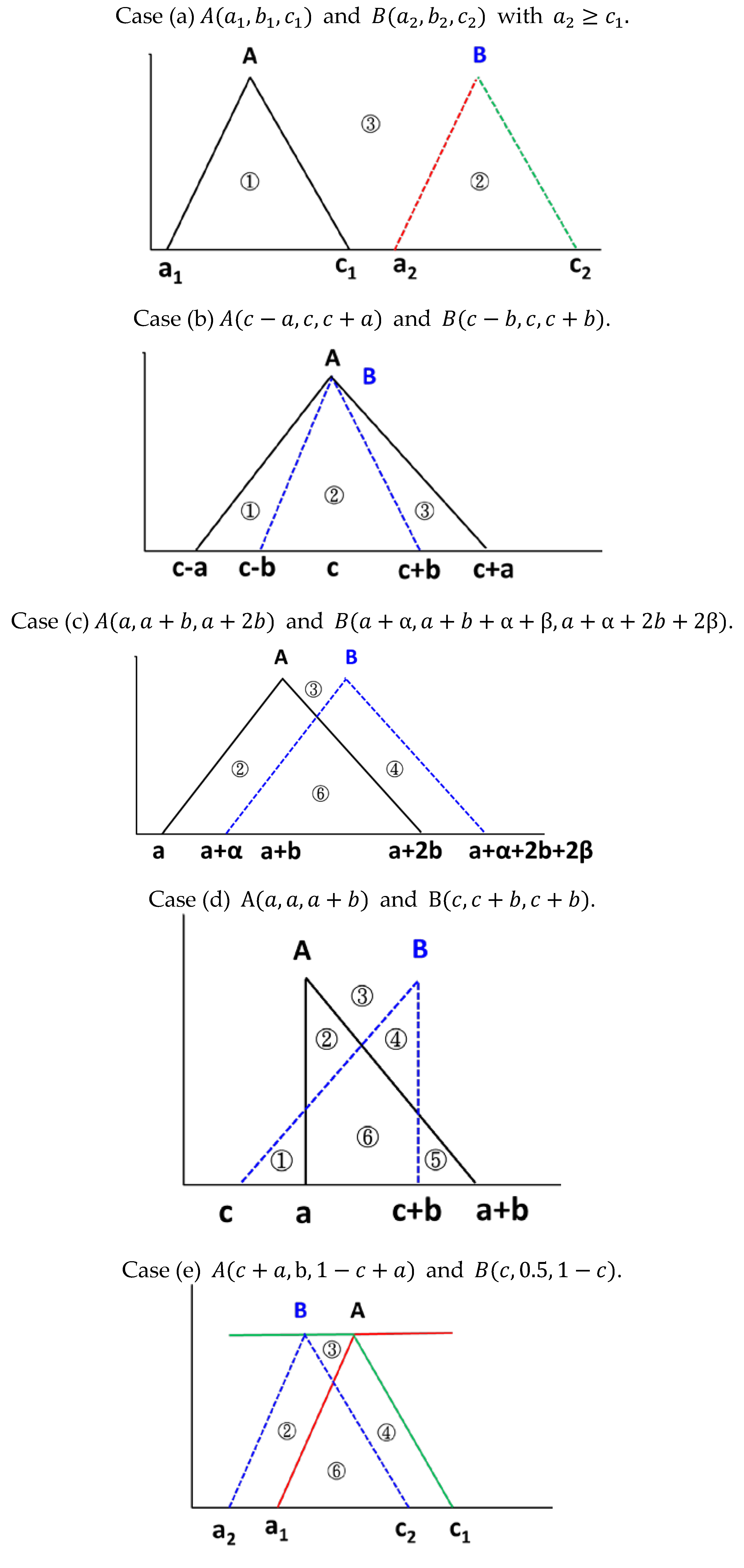
For the two triangular fuzzy numbers $A\left(a_1,b_1,c_1\right)$ and $B\left(a_2,b_2,c_2\right)$, the second comparative study is comprised of the five case studies shown in Figure 2, which compares the fuzzy preference relations $K1\prime \left(A,B\right)$, $K2\prime \left(A,B\right)$, $T1\prime \left(A,B\right)$ and $T2\prime \left(A,B\right)$.

Case (a) $A\left(a_1,b_1,c_1\right)$ and $B\left(a_2,b_2,c_2\right)$ with $a_2\ge c_1$.

It follows that:

$$\begin{gathered} K1\prime \left(A,B\right)=\frac{\left(Q_1+Q_3\right)+\left(Q_2+Q_3\right)+0}{\left(Q_1+Q_3\right)+\left(Q_2+Q_3\right)+0}=1 \\ K{2}^{\prime }\left(A,B\right)=\frac{\left(Q_1+Q_3\right)+\left(Q_2+Q_3\right)}{\left(Q_1+Q_3\right)+\left(Q_2+Q_3\right)}=1 \\ T1\prime \left(A,B\right)=\frac{0+\left(Q_1+Q_2\right)}{\left(Q_1+Q_2\right)}=1 \end{gathered}$$

and:

$$T2\prime \left(A,B\right)=\frac{\left(Q_1+Q_2\right)}{\left(Q_1+Q_2\right)}=1.$$

(1)

For this simple case, all the preference relations give the same degree of preference of B over A.

Case (b) $A\left(c-a,c,c+a\right)$ and $B\left(c-b,c,c+b\right)$.

We have:

$$\begin{gathered} K1\prime \left(A,B\right)=\frac{Q_1+0+Q_2}{Q_1+Q_3+2Q_2}=1/2 \\ K{2}^{\prime }\left(A,B\right)=\frac{Q_1+0}{Q_1+Q_3}=1/2 \\ T1\prime \left(A,B\right)=\frac{Q_2+Q_1}{(Q_1+Q_2+Q_3)+Q_2}=1/2 \end{gathered}$$

and:

$$T2\prime \left(A,B\right)=\frac{Q_1}{Q_1+Q_3}=1/2.$$

From the viewpoint of probability, the fuzzy numbers A and B have the same mean, but B has a smaller standard deviation. The results indicate that the differences between the decomposition and intersection of A and B cannot affect the degree of preference for B over A.

Case (c) $A\left(a,a+b,a+2b\right)$ and $B\left(a+\mathsf{\alpha },a+b+\mathsf{\alpha }+\mathsf{\beta },a+\mathsf{\alpha }+2b+2\mathsf{\beta }\right)$.

For this case, the fuzzy number B is a right shift of A. Therefore, B should have a higher ranking than A based on the intuition criterion. We obtain:

$$\begin{gathered} K1\prime \left(A,B\right)=\frac{(Q_2+Q_3)+\left(Q_3+Q_4\right)+Q_6}{(Q_2+Q_3)+\left(Q_3+Q_4\right)+2Q_6}=\frac{{\left(2b+\alpha +2\beta \right)}^2}{2\left({\alpha }^2+4b^2+4b\beta +2b\alpha +2{\beta }^2\right)}>1/2 \\ K{2}^{\prime }\left(A,B\right)=\frac{(Q_2+Q_3)+\left(Q_3+Q_4\right)}{(Q_2+Q_3)+\left(Q_3+Q_4\right)}=1 \\ T1\prime \left(A,B\right)=\frac{Q_6+\left(Q_2+Q_4\right)}{(Q_2+Q_6)+\left(Q_6+Q_4\right)}=1-\frac{{\left(-2b+\alpha \right)}^2}{2{(2b+\beta )}^2} \end{gathered}$$

and:

$$T2\prime \left(A,B\right)=\frac{Q_2+Q_4}{Q_2+Q_4}=1.$$

All methods prefer B, but $T1\prime \left(A,B\right)$ is indecisive. More precisely,

• If $2b+\beta <\alpha$, then $T1\prime \left(A,B\right)<1/2$, so $A>B$
• If $2b+\beta =\alpha$, then $T1\prime \left(A,B\right)=1/2$, so $A=B$
• If $2b+\beta >\alpha$, then $T1\prime \left(A,B\right)>1/2$, so $A<B$.

Hence, a conflicting ranking order of $T1\prime \left(A,B\right)$ exists in this case.

Case (d) $A\left(a,a,a+b\right)$ and $B\left(c,c+b,c+b\right)$ with $a\ge c$.

This case is more complex for the partial overlap of A and B. The membership function of B has the right peak, B expands to the left of A for the left membership function, and A expands to the right of B for the right membership function. We have:

$$\begin{gathered} K1\prime \left(A,B\right)=\frac{(Q_2+Q_3)+\left(Q_3+Q_4\right)+Q_6}{(Q_1+Q_2+Q_3)+\left(Q_3+Q_4+Q_5\right)+2Q_6}=0.5+\frac{b\left(-2a+b+2c\right)}{a^2+3b^2+2bc+c^2-2ab-2ac} \\ K{2}^{\prime }\left(A,B\right)=\frac{(Q_2+Q_3)+\left(Q_3+Q_4\right)}{(Q_1+Q_2+Q_3)+\left(Q_3+Q_4+Q_5\right)}=\frac{{(-a+b+c)}^2}{2a^2+b^2+2bc+2c^2-2ab-4ac} \\ T1\prime \left(A,B\right)=\frac{Q_6+\left(Q_2+Q_4\right)}{(Q_2+Q_5+Q_6)+\left(Q_1+Q_6+Q_4\right)}=\frac{\left(a+3b-c\right)\left(-a+b+c\right)}{4b^2} \end{gathered}$$

and:

$$T2\prime \left(A,B\right)=\frac{Q_2+Q_4}{Q_1+Q_2+Q_4+Q_5}=\frac{{(-a+b+c)}^2}{3a^2+b^2+2bc+3c^2-2ab-6ac}.$$

It follows that:

• If $-2a+b+2c<0$, then $K1\prime \left(A,B\right)<1/2$ and $K{2}^{\prime }\left(A,B\right)<1/2$, so $A>B$;
• If $-2a+b+2c=0$, then $K1\prime \left(A,B\right)=1/2$ and $K{2}^{\prime }\left(A,B\right)=1/2$, so $A=B$;
• If $-2a+b+2c>0$, then $K1\prime \left(A,B\right)>1/2$ and $K{2}^{\prime }\left(A,B\right)>1/2$, so $A<B$;
• If $b<\left(1+\sqrt{2}\right)\left(a-c\right)$, then $T1\prime \left(A,B\right)<1/2$ and $T2\prime \left(A,B\right)<1/2$, so $A>B$;
• If $b=\left(1+\sqrt{2}\right)\left(a-c\right)$, then $T1\prime \left(A,B\right)=1/2$ and $T2\prime \left(A,B\right)=1/2$, so $A=B$;
• If $b>\left(1+\sqrt{2}\right)\left(a-c\right)$, then $T1\prime \left(A,B\right)>1/2$ and $T2\prime \left(A,B\right)>1/2$, so $A<B$.

Three special subcases are considered as follows:

(1)

Subcase (d1) If $b=\left(1+\sqrt{2}\right)\left(a-c\right)$, then $A\left(a,a,\left(2+\sqrt{2}\right)a-\left(1+\sqrt{2}\right)c\right)$ and $B\left(c,\left(1+\sqrt{2}\right)a-\sqrt{2}c,\left(1+\sqrt{2}\right)a-\sqrt{2}c\right)$, therefore $T1\prime \left(A,B\right)=T2\prime \left(A,B\right)=0.5$, so $A=B$. However, $K1\prime \left(A,B\right)=\frac{6-\sqrt{2}}{8}$, $K{2}^{\prime }\left(A,B\right)=2/3$ and $A<B$.

(2)

Subcase (d2) If $b=2\left(a-c\right)$, then $A\left(a,a,3a-2c\right)$ and $B\left(c,2a-c,2a-c\right)$, therefore $T1\prime \left(A,B\right)=7/16$, $T2\prime \left(A,B\right)=1/3$, so $A>B$. However, $K1\prime \left(A,B\right)=K{2}^{\prime }\left(A,B\right)=0.5$ and $A=B$.

(3)

Subcase (d3) If $A\left(0.3,0.3,0.9\right)$ and $B\left(0.1,0.7,0.7\right)$, then $K1\prime \left(A,B\right)=0.5556$, $K{2}^{\prime }\left(A,B\right)=0.6667$, $T1\prime \left(A,B\right)=0.5556$, $T2\prime \left(A,B\right)=0.6667$, so $A<B$.

Therefore, if $b<2\left(a-c\right)$, then $K1\prime \left(A,B\right)<1/2$, $K{2}^{\prime }\left(A,B\right)<1/2$, $T1\prime \left(A,B\right)<1/2$ and $T2\prime \left(A,B\right)<1/2$, so $A>B$; if $b>\left(1+\sqrt{2}\right)\left(a-c\right)$, then $K1\prime \left(A,B\right)>1/2$, $K{2}^{\prime }\left(A,B\right)>1/2$, $T1\prime \left(A,B\right)>1/2$ and $T2\prime \left(A,B\right)>1/2$, so $A<B$.

Case (e) $A\left(c+a,\mathrm{b},1-c+a\right)$ and $B\left(c,0.5,1-c\right)$.

For this case, the membership function B is symmetric with respect to $x=0.5$. The membership function of A is parallel translation of that of B except its peak. We have the following results:

(1)

$K1\prime \left(A,B\right)=\frac{(Q_2+Q_3)+\left(Q_3+Q_4\right)+Q_6}{(Q_1+Q_2+Q_3)+\left(Q_3+Q_4+Q_5\right)+2Q_6}=\frac{5-8b-12c+8bc-2a^2+4b^2+8c^2}{7+4a-8b-20c-8ac+8bc+4b^2+16c^2}$. If $(1-2a-2b)(3+2a-2b-4c)<0$, then $K{1}^{\prime }\left(A,B\right)<1/2$, so $A>B$. For simplicity, the other two conditions are omitted.

(2)

$K{2}^{\prime }\left(A,B\right)=\frac{(Q_2+Q_3)+\left(Q_3+Q_4\right)}{(Q_1+Q_2+Q_3)+\left(Q_3+Q_4+Q_5\right)}=\frac{{(1-2b)}^2}{4a^2+{(1-2b)}^2}$. If $2a+2b-1>0$, then $K{2}^{\prime }\left(A,B\right)<1/2$, so $A>B$.

(3)

$T1\prime \left(A,B\right)=\frac{Q_6+\left(Q_2+Q_4\right)}{(Q_2+Q_5+Q_6)+\left(Q_1+Q_6+Q_4\right)}=\frac{2(1-b-c)(1-2c)-a^2}{2(1+2a-2b)(3+2a-2b-4c)(1-2c)}$ and $T2\prime \left(A,B\right)=\frac{Q_2+Q_4}{Q_1+Q_2+Q_4+Q_5}=\frac{{(1-2b)}^2\left(1-2c\right)}{4a^3+{(1-2b)}^2\left(1-2c\right)+a^2\left(6-4b-8c\right)}$. If $>-0.5+c+$ $\frac{1}{2}\sqrt{\left(1-2c\right)\left(3-4b-2c\right)}$, then $T1\prime \left(A,B\right)<1/2$ and $T2\prime \left(A,B\right)<1/2$, so $A>B$.

Four special subcases are considered as follows:

(1)

Subcase (e1) If $a=-0.5+c+\frac{1}{2}\sqrt{\left(1-2c\right)\left(3-4b-2c\right)}$, then $T1\prime \left(A,B\right)=T2\prime \left(A,B\right)=0.5$, so $A=B$. However, $K1\prime \left(A,B\right)>0.5$, $K{2}^{\prime }\left(A,B\right)>0.5$ and $A<B$.

(2)

Subcase (e2) If $2a+2b-1=0$, then $T1\prime \left(A,B\right)=0.5-\frac{{\left(1-2b\right)}^2}{16\left(1-b-c\right)\left(1-2c\right)}<0.5$, $T2\prime \left(A,B\right)=\frac{\left(1-2c\right)}{\left(3-2b-4c\right)}<0.5$, so $A>B$. However, $K1\prime \left(A,B\right)=K{2}^{\prime }\left(A,B\right)=0.5$ and $A=B$.

(3)

Subcase (e3) If $\mathrm{A}\left(0.3,0.4,0.9\right)$ and $\mathrm{B}\left(0.2,0.5,0.8\right)$, then $K1\prime \left(A,B\right)=0.4896$, $K{2}^{\prime }\left(A,B\right)=0.4286$, $T1\prime \left(A,B\right)=0.4896$, $T2\prime \left(A,B\right)=0.4286$, so $A>B$.

(4)

Subcase (e4) If $b\ge 0.5$, then $(1-2a-2b)(3+2a-2b-4c)<0$, $2a+2b-1>0$ and $a>-0.5+c+\frac{1}{2}\sqrt{\left(1-2c\right)\left(3-4b-2c\right)}$, so $K{1}^{\prime }\left(A,B\right)<1/2$, $K{2}^{\prime }\left(A,B\right)<1/2$, $T1\prime \left(A,B\right)<1/2$ and $T2\prime \left(A,B\right)<1/2$, hence $A>B$.

6. Conclusions

This paper analyzes and compares two types of Nakamura’s fuzzy preference relations—($N\left(A,B\right)$ and $N\prime \left(A,B\right)$)—two types of Kołodziejczyk’s fuzzy preference relations—($K1\prime \left(A,B\right)$ and $K2\prime \left(A,B\right)$)—and the counterparts of the Kołodziejczyk’s fuzzy preference relations—($T1\prime \left(A,B\right)$ and $T2\prime \left(A,B\right)$)—on a group of eight selected cases, with all the possible levels of overlap between two triangular fuzzy numbers $A\left(a_1,b_1,c_1\right)$ and $B\left(a_2,b_2,c_2\right)$. First, for $N\left(A,B\right)$ and $N\prime \left(A,B\right)$ we obtain that $N_j\left(A,B\right)+N_{8-j}\left(A,B\right)=1$, $j=1,2,3,4$. If $a_2+2b_2+c_2\ge a_1-2b_1-c_1$, we have that $1-N_j^{\prime }\left(A,B\right)\ge N_j\left(A,B\right)$ for $j=1,3,5,7$ and $1-N_j^{\prime }\left(A,B\right)\le N_j\left(A,B\right)$ for $j=2,4,6,8$. Secondly, for $K1\prime \left(A,B\right)$ and $K2\prime \left(A,B\right)$, we have that $K{1}_1^{\prime }\left(A,B\right)=K{1}_j^{\prime }\left(A,B\right)$ for $j=3,5,7$ and $K{1}_2^{\prime }\left(A,B\right)=K{1}_j^{\prime }\left(A,B\right)$ for $j=4,6,8$. Furthermore, $K{1}_1^{\prime }\left(A,B\right)+K{1}_2^{\prime }\left(A,B\right)=0$ for $b_1=b_2$ and $c_2=a_1$ and $K{1}_1^{\prime }\left(A,B\right)+K{1}_2^{\prime }\left(A,B\right)=1$ for $b_1=b_2$ and $c_1-a_2=c_2-a_1$. Thirdly, for test case 1, $T1\prime \left(A,B\right)\le K1\prime \left(A,B\right)\le K2\prime \left(A,B\right)=T2\prime \left(A,B\right)=1$. For the test cases 3, 5 and 7, if $a_2+2b_2+c_2\le a_1+2b_1+c_1$, then $K1\prime \left(A,B\right)\ge K2\prime \left(A,B\right)\ge T2\prime \left(A,B\right)$ and $K1\prime \left(A,B\right)\ge T1\prime \left(A,B\right)\ge T2\prime \left(A,B\right)$. For the test case 8, we have $K2\prime \left(A,B\right)=T2\prime \left(A,B\right)=0\le K1\prime \left(A,B\right)\le T1\prime \left(A,B\right)$. For the test cases 2, 4 and 6, if $a_2+2b_2+c_2\ge a_1+2b_1+c_1$, then $K1\prime \left(A,B\right)\le K2\prime \left(A,B\right)\le T2\prime \left(A,B\right)$ and $K1\prime \left(A,B\right)\le T1\prime \left(A,B\right)\le T2\prime \left(A,B\right)$. These results provide insights into the decomposition and intersection of fuzzy numbers. Among the six fuzzy preference relations, the appropriate fuzzy preference relation can be chosen from the decision-maker’s perspective. Given this fuzzy preference relation, the final ranking of a set of alternatives is derived.

Worthy of future research is extending the analysis to other types of fuzzy numbers. First, the analysis can be easily extended to the trapezoidal fuzzy numbers. Second, for the hesitant fuzzy set lexicographical ordering method, Liu et al. [14] modified the method of Farhadinia [15] and this was more reasonable in more general cases. Recently, Alcantud and Torra [16] provided the necessary tools for the hesitant fuzzy preference relations. Thus, the analysis of hesitant fuzzy preference relations is a subject of considerable ongoing research.

References

1. Chen, S.J.; Hwang, C.L. Fuzzy Multiple Attribute Decision-Making; Springer: Berlin, Germany, 1992. [Google Scholar]
2. Wang, X.; Kerre, E.E. Reasonable properties for the ordering of fuzzy quantities (I). Fuzzy Sets Syst. 2001, 118, 375–385. [Google Scholar] [CrossRef]
3. Wang, X.; Kerre, E.E. Reasonable properties for the ordering of fuzzy quantities (II). Fuzzy Sets Syst. 2001, 118, 387–405. [Google Scholar] [CrossRef]
4. Nakamura, K. Preference relations on a set of fuzzy utilities as a basis for decision-making. Fuzzy Sets Syst. 1986, 20, 147–162. [Google Scholar] [CrossRef]
5. Kolodziejczyk, W. Orlovsky’s concept of decision-making with fuzzy preference relation-further results. Fuzzy Sets Syst. 1990, 19, 197–212. [Google Scholar] [CrossRef]
6. Yuan, Y. Criteria for evaluating fuzzy ranking methods. Fuzzy Sets Syst. 1991, 44, 139–157. [Google Scholar] [CrossRef]
7. Li, R.J. Fuzzy method in group decision-making. Comput. Math. Appl. 1999, 38, 91–101. [Google Scholar] [CrossRef]
8. Lee, H.S. On fuzzy preference relation in group decision-making. Int. J. Comput. Math. 2005, 82, 133–140. [Google Scholar] [CrossRef]
9. Wang, Z.X.; Liu, Y.J.; Fan, Z.P.; Feng, B. Ranking LR fuzzy number based on deviation degree. Inf. Sci. 2009, 179, 2070–2077. [Google Scholar] [CrossRef]
10. Asady, B. The revised method of ranking LR fuzzy number based on deviation degree. Expert Syst. Appl. 2010, 37, 5056–5060. [Google Scholar] [CrossRef]
11. Zhang, F.; Ignatius, J.; Lim, C.P.; Zhao, Y. A new method for ranking fuzzy numbers and its application to group decision-making. Appl. Math. Model. 2014, 38, 1563–1582. [Google Scholar] [CrossRef]
12. Zhu, B.; Xu, Z.; Xu, J. Deriving a ranking from hesitant fuzzy preference relations under group decision-making. IEEE Tran. Cyber. 2014, 44, 1328–1337. [Google Scholar] [CrossRef] [PubMed]
13. Wang, Y.J. Ranking triangle and trapezoidal fuzzy numbers based on the relative preference relation. Appl. Math. Model. 2015, 39, 586–599. [Google Scholar] [CrossRef]
14. Liu, X.; Wang, Z.; Zhang, S. A modification on the hesitant fuzzy set lexicographical ranking method. Symmetry 2016, 8, 153. [Google Scholar] [CrossRef]
15. Farhadinia, B. Hesitant fuzzy set lexicographical ordering and its application to multi-attribute decision-making. Inf. Sci. 2016, 327, 233–245. [Google Scholar] [CrossRef]
16. Alcantud, J.C.R.; Torra, V. Decomposition theorems and extension principles for hesitant fuzzy sets. Inf. Fus. 2018, 41, 48–56. [Google Scholar] [CrossRef]
Figure 1. Eight test cases for two fuzzy numbers A ( a 1 , b 1 , c 1 ) and B ( a 2 , b 2 , c 2 ) .
Symmetry 09 00228 g001aSymmetry 09 00228 g001bSymmetry 09 00228 g001c
Figure 2. Five case studies of A and B for K 1 ( A , B ) , K 2 ( A , B ) , T 1 ( A , B ) and T 2 ( A , B ) .
Symmetry 09 00228 g002