
Analytical Solutions of Temporal Evolution of Populations in Optically-Pumped Atoms with Circularly Polarized Light

Abstract
:1. Introduction
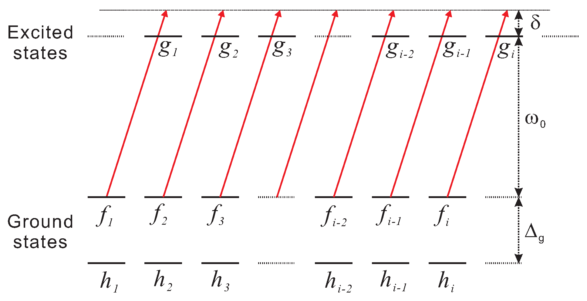
2. Theory
3. Calculated Results
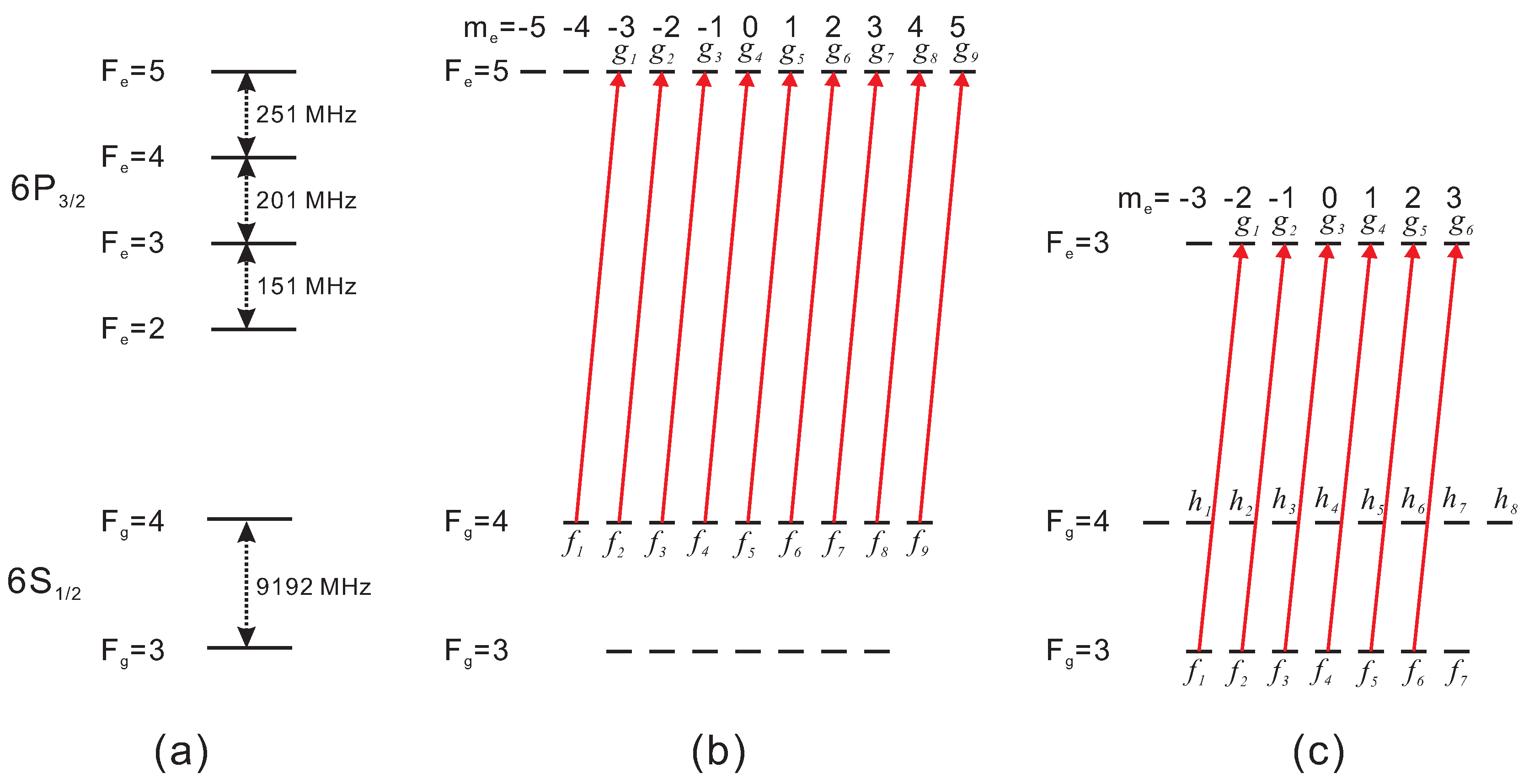
3.1. Results for the Transition
3.2. Results for the Transition
4. Conclusions
Acknowledgments
Conflicts of Interest
Appendix
References
- Happer, W. Optical pumping. Rev. Mod. Phys. 1972, 44, 169–249. [Google Scholar] [CrossRef]
- McClelland, J.J. Optical State Preparation of Atoms. In Atomic, Molecular, and Optical Physics: Atoms and Molecules; Dunning, F.B., Hulet, R.G., Eds.; Academic Press: San Diego, CA, USA, 1995; pp. 145–170. [Google Scholar]
- Smith, D.A.; Hughes, I.G. The role of hyperfine pumping in multilevel systems exhibiting saturated absorption. Am. J. Phys. 2004, 72, 631–637. [Google Scholar] [CrossRef]
- Magnus, F.; Boatwright, A.L.; Flodin, A.; Shiell, R.C. Optical pumping and electromagnetically induced transparency in a lithium vapour. J. Opt. B: Quantum Semiclass. Opt. 2005, 7, 109–118. [Google Scholar] [CrossRef]
- Han, H.S.; Jeong, J.E.; Cho, D. Line shape of a transition between two levels in a three-level Λ configuration. Phys. Rev. A 2011, 84. [Google Scholar] [CrossRef]
- Sydoryk, I.; Bezuglov, N.N.; Beterov, I.I.; Miculis, K.; Saks, E.; Janovs, A.; Spels, P.; Ekers, A. Broadening and intensity redistribution in the Na(3p) hyperfine excitation spectra due to optical pumping in the weak excitation limit. Phys. Rev. A 2008, 77. [Google Scholar] [CrossRef]
- Porfido, N.; Bezuglov, N.N.; Bruvelis, M.; Shayeganrad, G.; Birindelli, S.; Tantussi, F.; Guerri, I.; Viteau, M.; Fioretti, A.; Ciampini, D.; et al. Nonlinear effects in optical pumping of a cold and slow atomic beam. Phys. Rev. A 2015, 92. [Google Scholar] [CrossRef]
- McClelland, J.J.; Kelley, M.H. Detailed look at aspects of optical pumping in sodium. Phys. Rev. A 1985, 31, 3704–3710. [Google Scholar] [CrossRef] [PubMed]
- Farrell, P.M.; MacGillivary, W.R.; Standage, M.C. Quantum-electrodynamic calculation of hyperfine-state populations in atomic sodium. Phys. Rev. A 1988, 37, 4240–4251. [Google Scholar] [CrossRef] [PubMed]
- Balykin, V.I. Cyclic interaction of Na atoms with circularly polarized laser radiation. Opt. Commun. 1980, 33, 31–36. [Google Scholar] [CrossRef]
- Liu, S.; Zhang, Y.; Fan, D.; Wu, H.; Yuan, P. Selective optical pumping process in Doppler-broadened atoms. Appl. Opt. 2011, 50, 1620–1624. [Google Scholar] [CrossRef] [PubMed]
- Moon, G.; Shin, S.R.; Noh, H.R. Analytic solutions for the populations of an optically-pumped multilevel atom. J. Korean Phys. Soc. 2008, 53, 552–557. [Google Scholar] [CrossRef]
- Moon, G.; Heo, M.S.; Shin, S.R.; Noh, H.R.; Jhe, W. Calculation of analytic populations for a multilevel atom at low laser intensity. Phys. Rev. A 2008, 78. [Google Scholar] [CrossRef]
- Won, J.Y.; Jeong, T.; Noh, H.R. Analytical solutions of the time-evolution of the populations for D1 transition line of the optically-pumped alkali-metal atoms with I = 3/2. Optik 2013, 124, 451–455. [Google Scholar] [CrossRef]
- Noh, H.R. Analytical Study of Optical Pumping for the D1 Line of 85Rb Atoms. J. Korean Phys. Soc. 2104, 64, 1630–1635. [Google Scholar] [CrossRef]
- Moon, G.; Noh, H.R. Analytic solutions for the saturated absorption spectra. J. Opt. Soc. Am. B 2008, 25, 701–711. [Google Scholar] [CrossRef]
- Moon, G.; Noh, H.R. Analytic Solutions for the Saturated Absorption Spectrum of the 85Rb Atom with a Linearly Polarized Pump Beam. J. Korean Phys. Soc. 2009, 54, 13–22. [Google Scholar] [CrossRef]
- Do, H.D.; Heo, M.S.; Moon, G.; Noh, H.R.; Jhe, W. Analytic calculation of the lineshapes in polarization spectroscopy of rubidium. Opt. Commun. 2008, 281, 4042–4047. [Google Scholar] [CrossRef]
- Thornton, T.; Marion, J.B. Classical Dynamics of Particles and Systems, 5th ed.; Brooks/Cole: New York, NY, USA, 2004. [Google Scholar]
- Cohen-Tannoudji, C.; Dupont-Roc, J.; Grynberg, G. Atom–Photon Interactions Basic Processes and Applications; Wiley: New York, NY, USA, 1992. [Google Scholar]
- Meystre, P.; Sargent, M., III. Elements of Quantum Optics; Springer: New York, NY, USA, 2007. [Google Scholar]
- Metcalf, H.J.; van der Straten, P. Laser Cooling and Trapping; Springer: New York, NY, USA, 1999. [Google Scholar]

© 2016 by the author; licensee MDPI, Basel, Switzerland. This article is an open access article distributed under the terms and conditions of the Creative Commons by Attribution (CC-BY) license (http://creativecommons.org/licenses/by/4.0/).
Share and Cite
Noh, H.-R. Analytical Solutions of Temporal Evolution of Populations in Optically-Pumped Atoms with Circularly Polarized Light. Symmetry 2016, 8, 17. https://doi.org/10.3390/sym8030017
Noh H-R. Analytical Solutions of Temporal Evolution of Populations in Optically-Pumped Atoms with Circularly Polarized Light. Symmetry. 2016; 8(3):17. https://doi.org/10.3390/sym8030017
Chicago/Turabian StyleNoh, Heung-Ryoul. 2016. "Analytical Solutions of Temporal Evolution of Populations in Optically-Pumped Atoms with Circularly Polarized Light" Symmetry 8, no. 3: 17. https://doi.org/10.3390/sym8030017
APA StyleNoh, H.-R. (2016). Analytical Solutions of Temporal Evolution of Populations in Optically-Pumped Atoms with Circularly Polarized Light. Symmetry, 8(3), 17. https://doi.org/10.3390/sym8030017