Effects of Initial Symmetry on the Global Symmetry of One-Dimensional Legal Cellular Automata

Abstract
:1. Introduction
2. Methods
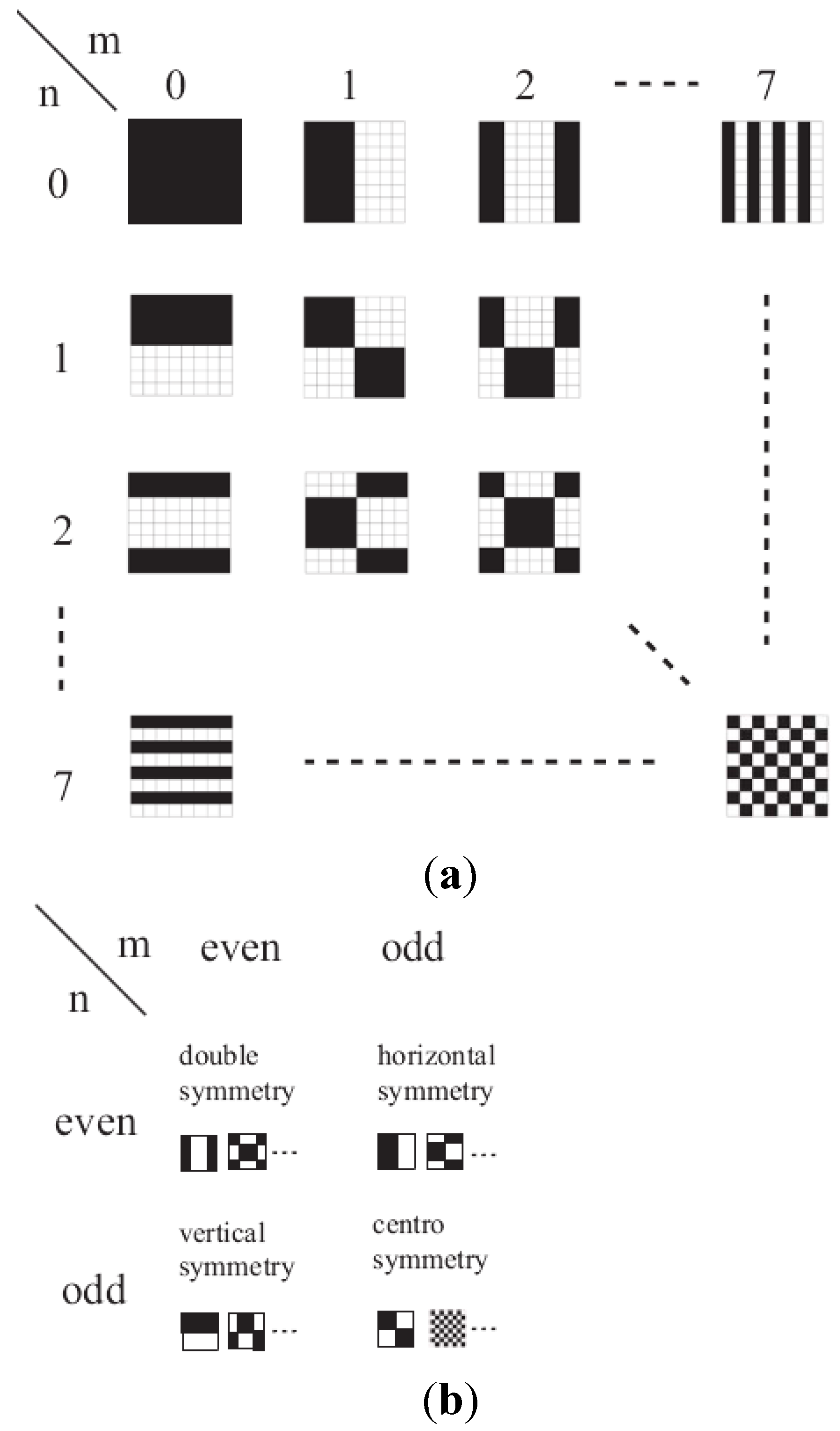
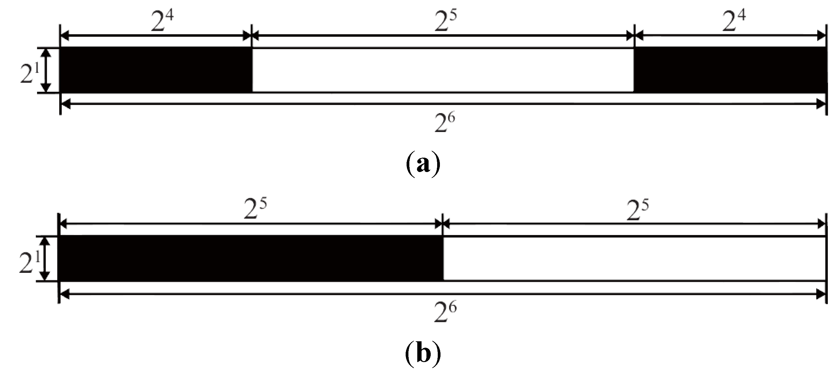
The Discrete Walsh Analysis
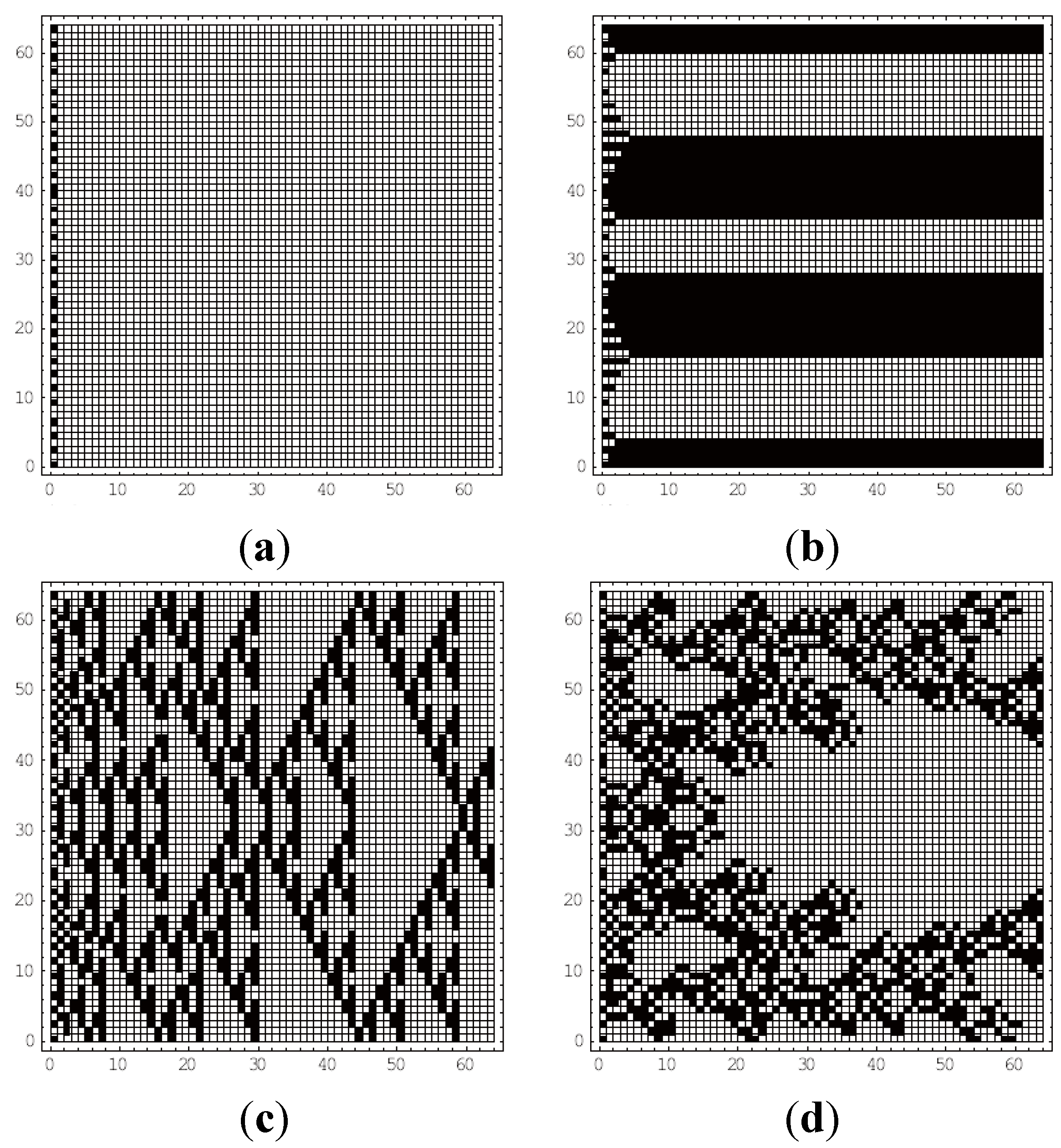
3. Calculations
4. Results
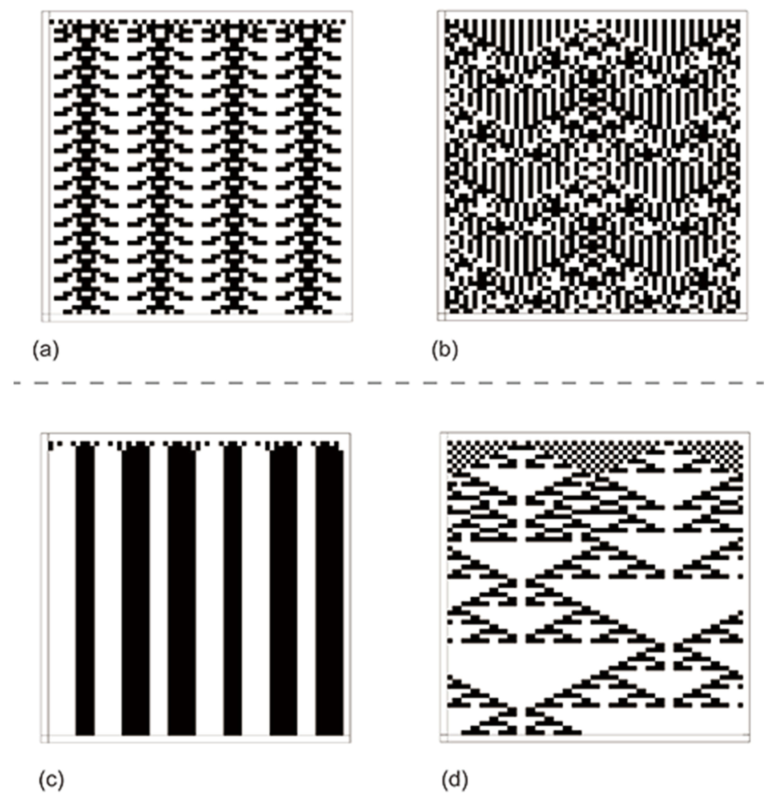
4.1. Class
4.2. Four Types of Symmetry
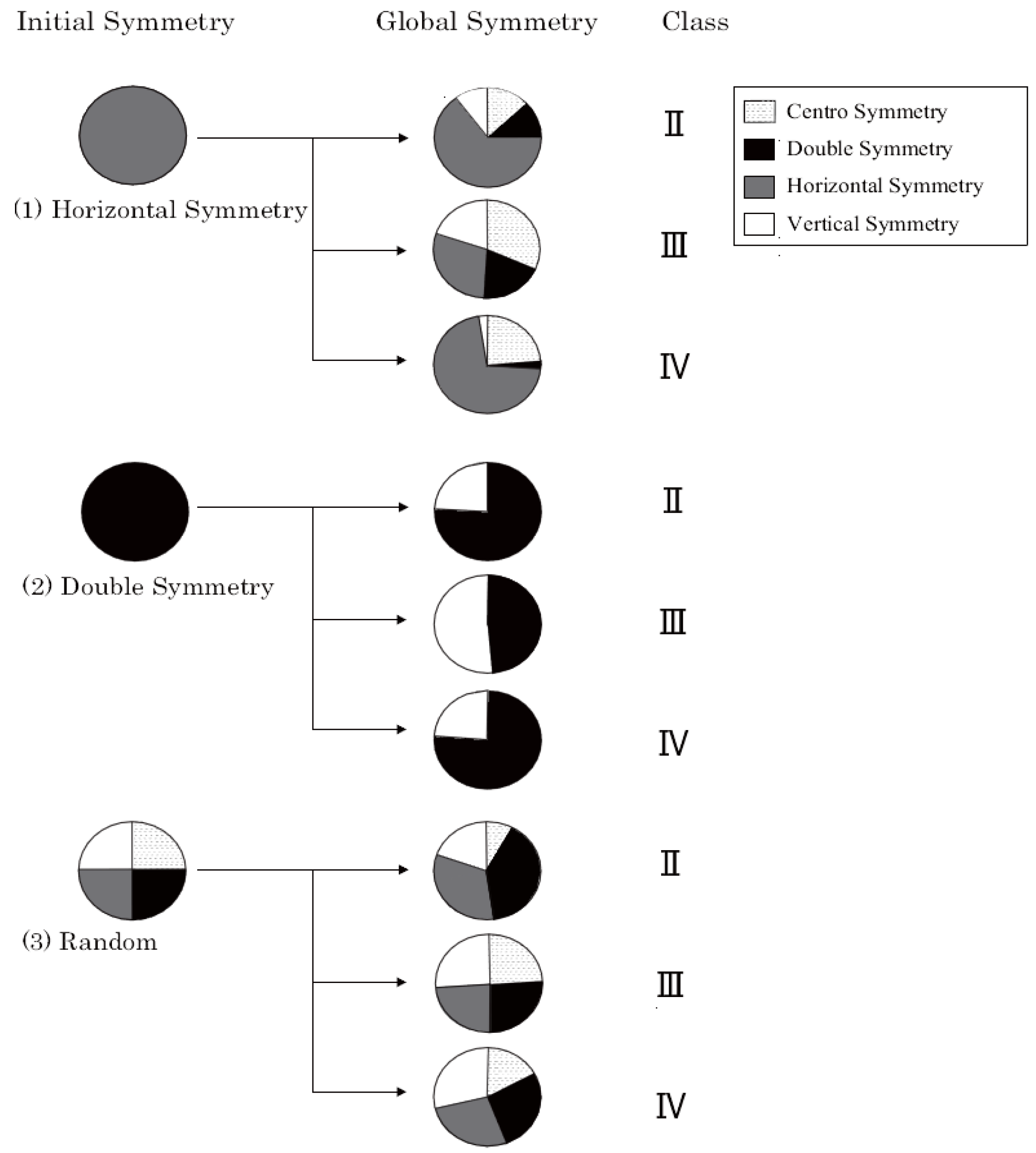

4.3. The Ratio of Final Formation

| Class | Horizontal Symmetry | Double Symmetry | Random |
|---|---|---|---|
| Periodic | 12 | 12 | 100× |
| Chaotic | 43 | 44 | 100× |
| Complex | 6 | 6 | 100× |
5. Discussion
5.1. Class
5.2. Four Types of Symmetry
5.3. The Ratio of Final Formation
6. Conclusions
Acknowledgements
Conflicts of Interest
References
- Allen, W.L.; Cuthill, I.C.; Scott-Samuel, N.E.; Baddeley, R. Why the leopard got its spots: Relating pattern development to ecology in felids. Proc. R Soc. B. 2010, 1373–1380. [Google Scholar] [CrossRef] [PubMed]
- Ubukata, T. Theoretical morphology of composite prismatic, fibrous prismatic and foliated microstructures in bivalves. Venus 2000, 59, 297–305. [Google Scholar]
- Nishiyama, Y.; Nanjo, K.Z.; Yamasaki, K. Geometrical minimum units of fracture patterns in two-dimensional space: Lattice and discrete Walsh functions. Phys. A 2008, 387, 6252–6262. [Google Scholar]
- Yamasaki, K.; Nanjo, K.Z.; Chiba, S. Symmetry and entropy of one-dimensional legal cellular automata. Complex Syst. 2012, 20, 352–361. [Google Scholar]
- Yamasaki, K.; Nanjo, K.Z.; Chiba, S. Symmetry and entropy of biological patterns: Discrete Walsh functions for 2D image analysis. BioSystems 2010, 103, 105–112. [Google Scholar] [CrossRef] [PubMed]
- Yodogawa, E. Symmetropy, an entropy-like measure of visual symmetry. Percept. Psychophys. 1982, 32, 230–240. [Google Scholar] [CrossRef] [PubMed]
- Wolfram, S. Universality and complexity, in cellular automata. Phys. D 1984, 10, 1–35. [Google Scholar] [CrossRef]
- Wolfram, S. A New Kind of Science; Wolfram Media, Inc.: Champaign, IL, USA, 2002. [Google Scholar]
- Martin, B. A Walsh exploration of Wolfram CA rules. In Proceedings of the 12th International Workshop on Cellular Automata, Hiroshima University, Higashi-Hiroshima, Japan, 12–15 September 2006; pp. 25–30.
- Stewart, I.; Golubitsky, M. Fearful Symmetry: Is God a Geometer? Blackwell Pub: Oxford, UK, 1992; p. 346. [Google Scholar]
- Schiff, J.L. Cellular Automata: Discrete View of the World; John Wiley & Sons Inc.: Hoboken, NJ, USA, 2008; p. 250. [Google Scholar]
- Peignon, J.M.; Gérard, A.; Naciri, Y.; Ledu, C.; Phélipot, P. Analyse du déterminisme de la coloration et de l'ornementation chez la palourde japonaise Ruditapes Philippinarum. Aqua. Liv. Res. 1995, 8, 181–185. (In French) [Google Scholar] [CrossRef]
- Akiyama, B.Y.; Saito, H.; Nanbu, R.; Tanaka, Y.; Kuwahara, H. The spatial distribution of Manila clam Ruditapes philippinarum associated with habitat environment in a sandy tidal flat on the coast of Matsunase, Mie Prefecture, Japan. Ecol. Civil. Eng. 2011, 14, 21–34. (In Japanese) [Google Scholar] [CrossRef]
- Habe, T. Gakken Picture Book of Shellfish; Gakken Holdings: Tokyo, Japan, 1975; p. 294. (In Japanese) [Google Scholar]
© 2015 by the authors; licensee MDPI, Basel, Switzerland. This article is an open access article distributed under the terms and conditions of the Creative Commons Attribution license (http://creativecommons.org/licenses/by/4.0/).
Share and Cite
Tanaka, I. Effects of Initial Symmetry on the Global Symmetry of One-Dimensional Legal Cellular Automata. Symmetry 2015, 7, 1768-1779. https://doi.org/10.3390/sym7041768
Tanaka I. Effects of Initial Symmetry on the Global Symmetry of One-Dimensional Legal Cellular Automata. Symmetry. 2015; 7(4):1768-1779. https://doi.org/10.3390/sym7041768
Chicago/Turabian StyleTanaka, Ikuko. 2015. "Effects of Initial Symmetry on the Global Symmetry of One-Dimensional Legal Cellular Automata" Symmetry 7, no. 4: 1768-1779. https://doi.org/10.3390/sym7041768
APA StyleTanaka, I. (2015). Effects of Initial Symmetry on the Global Symmetry of One-Dimensional Legal Cellular Automata. Symmetry, 7(4), 1768-1779. https://doi.org/10.3390/sym7041768