
Dihedral Reductions of Cyclic DNA Sequences

Abstract
: The data-analytic methodology of dihedral reductions for cyclic orbits of distinct-base codons is described both in terms of Fourier analysis over the dihedral groups and in (algebraically equivalent) terms of canonical projections. Numerical evaluations are presented for discrete and continuous scalar data indexed by cyclic orbits.1. Introduction
The role of group-theoretic arguments in biology has a long history, in which R.A. Fisher’s classification of segregation genotypes in the theory of polysomic inheritance is a classical example [1]. In the theory of experimental designs, it was also Fisher who demonstrated the explicit usefulness of cyclic groups in the theory of confounding in factorial experiments [2,3], now widely used in biology and genetics studies. In recent decades, the theory and applications of algebraic methods in statistics and probability became a well-established area of interest, e.g., [4,5].
In structural biology as well, applications of symmetry arguments have been used to formulate working hypotheses and to suggest explanation and prediction, e.g., [6–10]. An explicit connection between symmetry arguments and data analytic reasoning in structural biology can be exemplified by the study [11] of the evolutionary importance of purine and pyrimidine content in the human immunodeficiency virus type 1, based on the statistical assessment of the frequency diversity of cyclic sets, defined as the ratio
More specifically, the present communication is aimed at showing that there is a broader group-theoretic and data-analytic framework within which the methodology described in [11] can be identified and further utilized, thus leading to eventually richer biological interpretations and explanatory narratives.
The framework of interest (Symmetry Studies) was described originally in [12] and is briefly reviewed in [13]. We will also refer to [14] for notions of Fourier analysis over the finite groups relevant to the present applications. See also [15–18] for related discussions, and [19,20] for applications in the field of linear optics.
This paper is divided as follows. The basic definitions, assumptions and notations are introduced in the next section. The cyclic reductions are discussed in Section 3. Numerical evaluations are presented in Section 4. Additional background material is presented in Appendices A, B, and C.
2. Definitions, Assumptions and Notation
Any DNA sequence in length of ℓ base pairs (bp) can be represented as a point in the set of all mappings
In what follows, we will indicate by
Throughout this communication, sequences written in lower case will always indicate the cyclic orbit generated by the corresponding sequence, to be written in upper case. For example,
It follows directly from (4) that two sequences S and F are complementary if
2.1. Injective Sequences
The dihedral reductions to be considered in this communication are obtained for DNA sequences in length of three (or codons) composed of distinct bases {A,G,C,T}. That is, for the injective mappings into with domain L = {1, 2, 3}. These sequences account for the 24 distinct injective codons factored into 8 distinct cyclic orbits of length three.
Although the group actions (3)–(5) are defined for all mappings in , the resulting data-analytic applications may need to be adapted when non-injective sequences are included, due to the fact that the resulting actions may no longer be transitive. In that case, the data analysis is carried piecewise within the transitive parts [12]. In addition, because the actions on the injective sequences are faithful, any experimental results indexed by the points in the orbit are in one-to-one correspondence with the group elements, and can consequently be indexed by the group elements themselves. It is in the resulting group algebra structure that Fourier transforms can naturally be defined.
2.2. Scalar Measurements
Throughout this paper it will be opportune to distinguish the following types of experimental data:
Data indexed by sequences, , indicated by xS;
Data indexed by cyclic orbits, , indicated by xs;
Data indexed by group elements, , indicated by xτ, xσ,….
For example, the frequency diversity Equation (1) for act in terms of frequency counts xS over a given region of the genome is given by
2.3. Orbit Invariance
Every symmetry orbit has an intrinsic arbitrariness in the choice of its generating point, so that the resulting orbit is the same regardless of its generator. For example, recalling Equation (6),
Therefore, one would want the corresponding data summaries
A class of data summaries with this (orbit) invariance property, as shown in [14], is given precisely by the Fourier transforms
A class of (faithful) group actions on the cyclic orbits that allows us to identify xτ with xs and evaluate the Fourier transforms (or orbit invariants) will be introduced in the next section.
2.4. Dihedral Orbits
The dihedral groups Dn, for n = 3, 4, …, can be realized as the group
The action (3) under G = D3 gives four distinct dihedral orbits
Similarly, the action (3) under G = D4 gives three distinct dihedral orbits
3. Invariant Reductions
In Diagrams (10) and (11), D3 rotations and reversals are shown sideways along the rows of the diagrams and complementary orbits are shown along columns, so that each box is labeled by a cyclic orbit. We shall refer to the orbits in each of the diagrams simply as conjugated orbits.
In addition, each orbit is labeled by the polarity (⊕, ⊖) of the sequence’s strand and by the encoding sense (→) or anti-sense (←) direction with which a gene or protein product reads off the sequence. More specifically, following (10), if any point in the act orbit is labeled with a positive polarity and with a reading sense direction then:
The corresponding point in the tca orbit has positive polarity and the reading is in the anti-sense direction;
The corresponding point in the tga orbit has negative polarity and the reading is in the sense direction, and;
The corresponding point in the agt orbit has negative polarity and the reading is in the anti-sense direction.
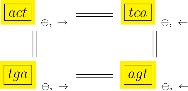
Diagram (11) shows the complementary orbits gct and agc, with the same polarity and direction interpretation as in Diagram (10).

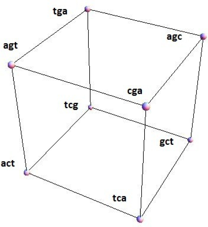
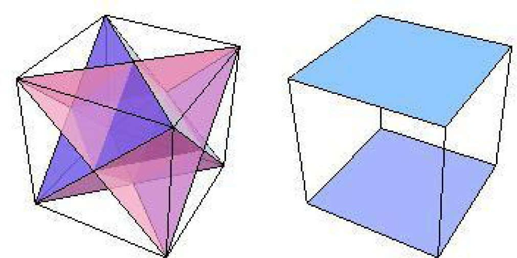
Figure 1 shows a configuration space for the conjugated cyclic orbits of Diagrams (10) and (11), relative to which Figure 2 shows, respectively on the left and right images, the common direction and common polarity configuration subspaces. In this configuration space (obviously not unique), same-direction subspaces span two intercepting tetrahedrons, whereas same-polarity subspaces span two parallel faces of the configuration space.
3.1. D2-Invariant Reductions
There is a transitive faithful action of C2 × C2 ≃ D2 on the cyclic orbits s of (10), given by

| τ | σ | act | tca | tga | agt |
|---|---|---|---|---|---|
| 1 | 1 | act | tca | tga | agt |
| 1 | (AT)(GC) | tga | agt | act | tca |
| (13) | 1 | tca | act | agt | tga |
| (13) | (AT)(GC) | agt | tga | tca | act |
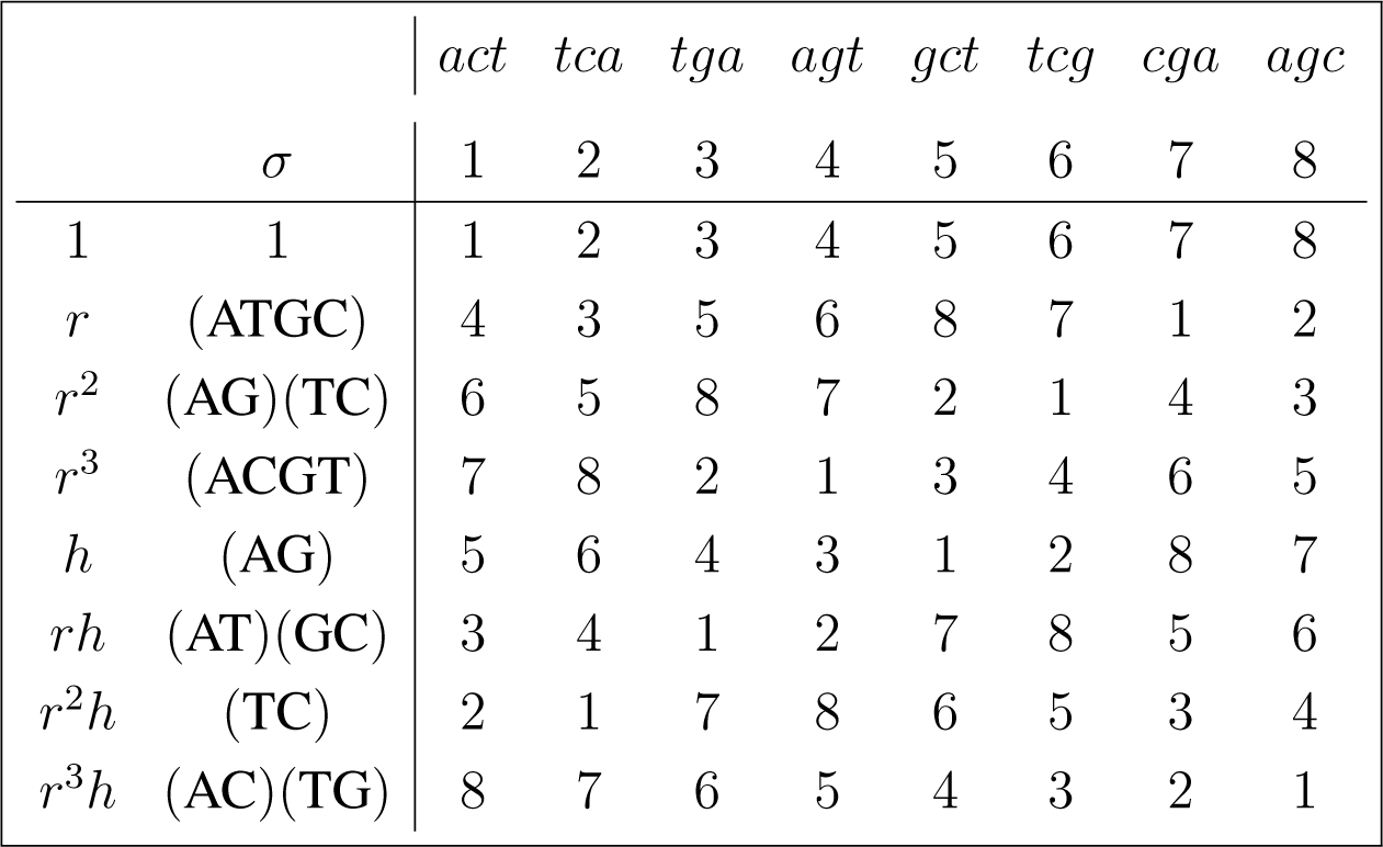
As a consequence, any experimental data xs indexed by the orbits (s) in the diagram can be reduced by the tools of dihedral Fourier analysis over D2. We emphasize that the transitiveness and faithfulness of the D2 action on the set of orbits is necessary to identify the orbits with the group elements and then proceed to the determination of the (D2) orbit invariants using the Fourier transforms. Following [14], these four one-dimensional transforms are simply
3.2. Entropy Invariants
The orbit invariants determined above are functions of any scalars xs obtained over the orbit s, such as its diversity (7), its raw sum (8), or its total molecular weight. When xs are positive integers, such as the sum of frequency counts over the orbit s, then the entropy (Ent ) of the observed distributions of frequency counts given by,
3.3. D4-Invariant Reductions
There are three non-equivalent transitive right actions σs of D4 on the set
D4 ≃< (ATGC), (AG) >,
D4 ≃< (AGCT), (AC) >,
D4 ≃< (ACTG), (AT) >.
The action of D4 ≃< (ATGC), (AG) > is given by:
3.4. Canonical Projections
The linear representation of D4 in defined by (16) is given by the permutation matrices associated with the rotations
Similarly, the action generated by D4 ≃< (AGCT), (AC) > yields a linear representation of
The resulting canonical projections , indexed by the irreducible representations
3.4.1. Interpretation of the Components
The particular representation (17) leads to the following interpretation of each of the non-trivial (orbit invariant) components of ‖x‖2, in terms of the combinations of polarity (⊕,⊖) and direction (→, ←),
The projection identifies a one-dimensional invariant comparing the overall mean effects
The projection identifies a one-dimensional invariant contrasting the same variation described above. Lastly, the projection identifies a two-dimensional invariant assessing direction given polarity effects in terms of
3.5. Dihedral Fourier Analysis
Reading from the column under the act orbit in (16), the points in the group algebra are given by
It is opportune to remark here that in the definition of Equation (21) we arbitrarily assigned the identity in D4 to xact. Any of the other potential assignments would be precisely a relabeling of the orbit’s starting point. The Fourier transforms, however, would remain orbit invariant, in the sense of Equation (9).
4. Numerical Evaluations
In this section we apply the cyclic reductions described in Section 3 to specific complete genomes of the human immunodeficiency virus type 1 and the hepatitis C virus.
4.1. Relative Entropy Study of the HIV1 BRUCG Isolate
Following Section 3.2, the data indexed by the cyclic orbits are simply the sums xs of the frequency counts xS with which the sequence S occurs in a given region of the genome, that is,
The frequency counts were evaluated by scanning the genome one base at a time in the 5′−3′ direction. The sequence in FASTA format was downloaded from the NCBI website ( http://www.ncbi.nlm.nih.gov). Computations were evaluated using the Symmetry Computing Toolbox (Symmetry Computing Toolbox, ⓒM.Viana). This particular HIV1 isolate, used here for numerical illustration only, also appears in the study of the HIV1’s evolutionary properties [11].
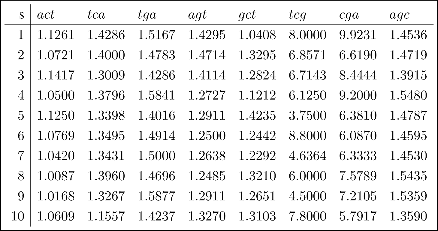
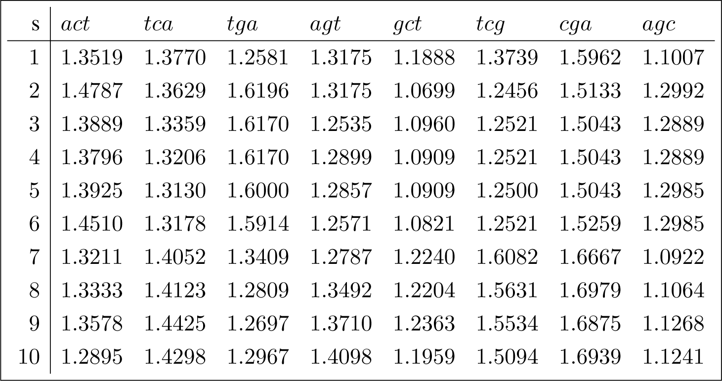
The frequency counts were obtained for the complete genome of human immunodeficiency virus type 1, isolate BRU (LAV-1), sequence ID gi:326417, accession number K02013.1, HIVBRUCG. See [23]. The full 9229 bp-long sequence was partitioned into six equal-length adjacent regions numbered 1–6, where the cyclic summaries xs were evaluated. The frequency counts for the conjugated cyclic orbits of act corresponding to Diagram (10) are shown in (22) and (23), whereas in (24) and (25) show the frequency counts for the conjugated cyclic orbits of gct corresponding to Diagram (11).

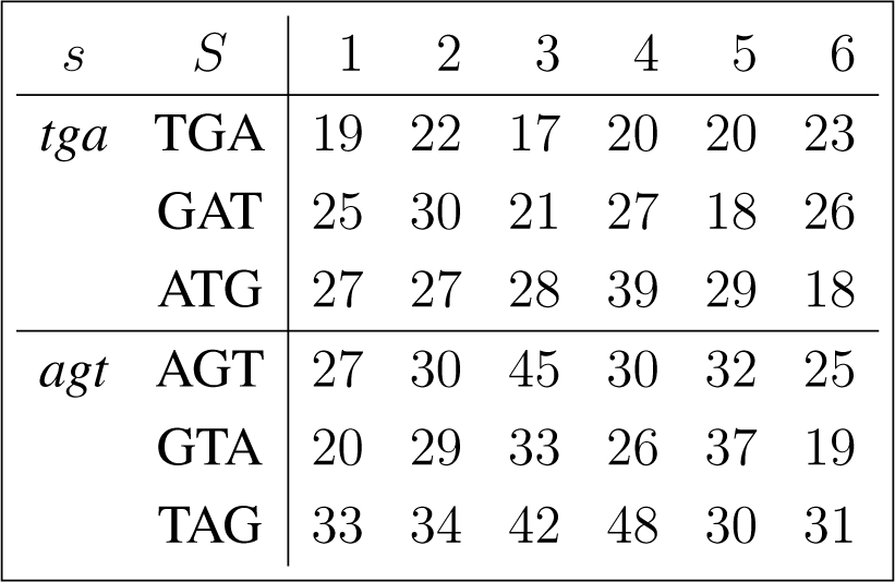
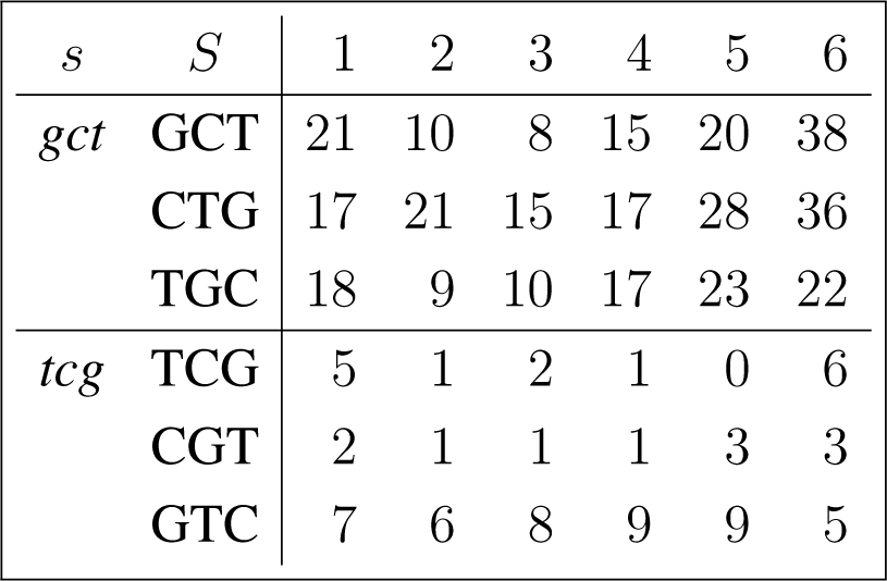
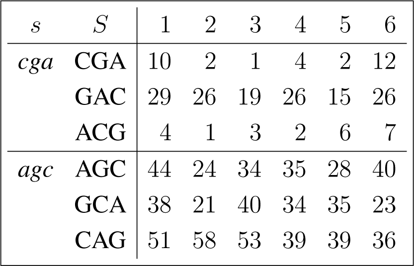
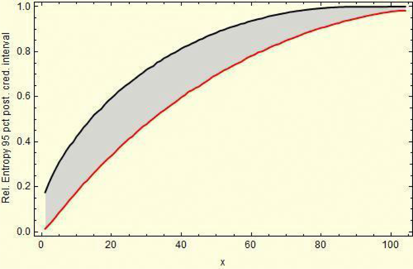
Figure 3 shows the resulting relative entropy invariants, as defined in Section 3.2, both for the act and for the gct conjugated cyclic orbits.
For example, reading from Region 3, in Equations (24) and (25), we have
Interpretations:
Reading again from Diagrams (10) and (11), it follows that the invariant
Polarity uncertainty: ;
Direction uncertainly: ;
Interaction: .
4.2. Statistical Assessment
The statistical assessment of the entropy can be obtained by numerically evaluating its sampling distribution based on 10,000 randomly generated observations from the posterior (Beta) distribution conjugated to binomial likelihood for the data, relative to the uniform prior probability distribution. Based on the resulting sampling distribution, a numerical evaluation of a posterior 95% credibility interval (CI) for the relative entropy can be obtained.
For example, reading from Region 5, in (24) and (25), we have,
4.3. Orbit Diversity Decomposition for the HIV1 Samples
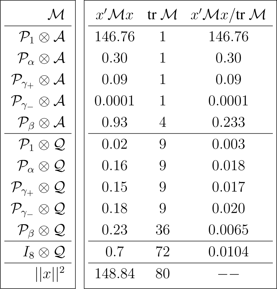
In this section we apply the canonical decomposition introduced in Section 3.4 and evaluated in Appendix C to reduce the diversity data shown in Equation (1) indexed by the joint set of conjugated orbits (the conjugated orbits of act adjoined to the conjugated orbits of gct), using the D4 action defined in Section 3.3. The orbit diversity for the joint set of conjugated orbits is shown in (26) for each sequence in the sample of 10 Brazilian sequences referenced in Appendix B.1.
The inclusion of the error (due to sampling variability) term in the canonical decomposition for the sample is obtained by tensoring the decomposition induced by the representation of interest, shown in Appendix C, with the standard canonical decomposition [12] (Chapter 4)
Because , and , we have
Similarly,
The degrees of freedom in each case are obtained by the traces of the corresponding projections, which are also equal to the dimension of the projecting (invariant) subspaces. Under suitable parametric assumptions the magnitude of the ratios

Under large-sample parametric assumptions and independent dihedral covariance structure it follows that, with the exception of the contrast associated with γ−, all F-ratios are significantly high (statistically distinct from zero).
4.4. Orbit Diversity Decomposition for the HCV Samples
This section replicates the methods described in Section 4.3 for a sample of 10 Brazilian hepatitis C sequences. The orbit diversity for the joint set of conjugated orbits for each sequence in the sample is shown in (28). Their accession numbers are referenced in Appendix B.1.
The corresponding analysis of variance decomposition is shown in (29).
It should be evident, by comparing the magnitude of the F-ratios,
| virus | ||||
|---|---|---|---|---|
| HIV1 | 238.342 | 5.889 | 1.882 | 137.962 |
| HCV | 28.846 | 8.653 | 0.009 | 22.115 |
5. Summary
In this communication we constructed dihedral D2 reduction of conjugate injective cyclic orbits in length of three, a dihedral D4 reduction of their combined set, and a dihedral D3 reduction of the set of conjugate injective cyclic orbits in length of four. In each case, the experimental scalar data can be any summary obtained over the cyclic orbits, such as the sum or an extreme value of the frequency counts over the cyclic orbit, the entropy of a frequency distribution over the orbit, its amino acid content, or, as in [11], the orbit’s frequency diversity. In the case of matrix data, the data-analytic methods of group rings, instead of group algebras would then be the appropriate methodology [14].
Acknowledgments
The author is thankful to the referees’ comments and clarifying suggestions.
Appendix
A. HIV1 and HCV Sequences
The following are the accession numbers for the HIV1 and HCV sequences considered in the present study:

B. Additional Studies
B.1. Relative Entropy Study of 10 Brazilian HIV1 Sequences
The relative entropy evaluations illustrated above in Section 4.1 were replicated for a sample of 10 Brazilian HIV1 sequences, referenced in Appendix A. The raw frequency counts and the corresponding relative entropy profiles for each of 10 sequences are linked in [24].
B.2. Relative Entropy Study of 10 Brazilian HCV Sequences
Similarly to the study for the HIV1, a sample of 10 Brazilian hepatitis C sequences was evaluated for their relative entropy. The sequences are referenced in Appendix A. The raw frequency counts and the corresponding relative entropy profiles along each genome are linked in [25]. The relative entropy invariant profiles clearly highlight the structural differences between the two types of viruses.
B.3. Relative Entropy Study of Random Reference Sequences
It is statistically useful to compare the cyclic reductions obtained for HIV1’s isolate described above with those from random DNA sequences of comparable lengths. The results, based on 20 random sequences, shown in [26], clearly indicate that the observed variations in relative entropy (invariants) for the conjugated gct orbits, both for HIV1 and HCV sequences, are well below what one would expect to observe for random sequences of comparable lengths.
C. Canonical Projections
The following are the canonical projections
Conflicts of Interest
The author declares no conflict of interest.
References
- Fisher, R.A. The theory of linkage in polysomic inheritance. Philos. Trans. Roy. Soc. London. Ser. B 1947, 233, 55–87. [Google Scholar]
- Fisher, R.A. The theory of confounding in factorial experiments in relation to the theory of groups. Ann. Eugen 1942, 11, 341–353. [Google Scholar]
- Fisher, R.A. A system of confounding for factors with more than two alternatives, giving completely orthogonal cubes and higher powers. Ann. Eugen 1945, 12, 283–290. [Google Scholar]
- Viana, M. Algebraic Methods in Statistics and Probability; Contemporary Mathematics; Richards, D., Ed.; American Mathematical Society: Providence, RI, USA, 2001; Volume 287. [Google Scholar]
- Viana, M. Algebraic Methods in Statistics and Probability II; Contemporary Mathematics; Wynn, H., Ed.; American Mathematical Society: Providence, RI, USA, 2010; Volume 516. [Google Scholar]
- Findley, G.L.; Findley, A.M.; McGlynn, S.P. Symmetry characteristics of the genetic code. Proc. Natl. Acad. Sci. USA 1982, 79, 7061–7065. [Google Scholar]
- Sergienko, I.V.; Gupal, A.M.; Vagis, A.A. Symmetry in encoding genetic information in DNA. Cybern. Syst. Anal 2011, 47, 408–414. [Google Scholar]
- Hornos, J.E.; Braggion, L.; Magini, M.; Forger, M. Symmetry preservation in the evolution of the genetic code. IUBMB Life 2004, 56, 125–130. [Google Scholar]
- Zandi, R.; Reguera, D.; Bruinsma, R.F.; Gelbart, W.M.; Rudnick, J.; Reiss, H. Origin of icosahedral symmetry in viruses. Proc. Natl. Acad. Sci. USA 2004, 101, 15556–15560. [Google Scholar]
- Finkel, D.L. HIV-1 ancestry primordial expansions of RRE and RRE- related sequences. J. Theor. Biol 1992, 3, 285–302. [Google Scholar]
- Doi, H. Importance of purine and pyramidine content of local nucleotide sequences (six bases long) for evolution of human immunodeficiency virus type 1. Evolution 1991, 88, 9282–9286. [Google Scholar]
- Viana, M. Symmetry Studies, an Introduction to the Analysis of Structured Data in Applications; Cambridge University Press: New York, NY, USA, 2008. [Google Scholar]
- Souza, D.J.; Chaves, L.M.; Viana, M.A.G. Symmetries in symbolic sequences. Rev. Bras. Biom 2010, 1, 73–86. [Google Scholar]
- Viana, M.; Lakshminarayanan, V. Dihedral Fourier Analysis, Data-Analytic Aspects and Applications; Lecture Notes in Statistics; Springer: New York, NY, USA, 2013; Volume 206. [Google Scholar]
- Viana, M. Canonical invariants for three-candidate preference rankings. Can. Appl. Math. Q 2007, 15, 203–222. [Google Scholar]
- Viana, M. Canonical Decompositions and Invariants for Data Analysis; Elsevier: Amsterdam, The Netherlands, 2009. [Google Scholar]
- Viana, M. Symmetry studies and decompositions of entropy. Entropy 2006, 8, 88–109. [Google Scholar]
- Viana, M. Symmetry orbits and their data-analytic properties. Rev. Mat 2013, 20, 155–166. [Google Scholar]
- Viana, M. Dihedral Polynomials. In Mathematical Optics: Classical, Quantum, and Computational Methods; Lakshminarayanan, V., Calvo, M.L., Alieva, T., Eds.; CRC Press: Boca Raton, FL, USA, 2012. [Google Scholar]
- Viana, M.; Lakhsminarayanan, V. Symmetry studies of refraction data. J. Modern Opt 2014, 61, 138–146. [Google Scholar]
- Viana, M. Symmetry-Related Decompositions of Uncertainty. Proceedings of the XI Brazilian Meeting on Bayesian Statistics, Amparo-SP, Brazil, 18–22 March 2012; Stern, J., Lauretto, M., Polpo, A., Diniz, M., Eds.; American Institute of Physics: Melville, NY, USA, 2012. [Google Scholar] [CrossRef]
- Cartan, E. The Theory of Spinors; MIT Press: Cambridge, MA, USA, 1966. [Google Scholar]
- Human immunodeficiency virus type 1, isolate BRU, complete genome (LAV-1), Available online: http://www.ncbi.nlm.nih.gov/nuccore/K02013.1 accessed on 23 December 2014.
- Relative entropy study of 10 Brazilian HIV1 sequences, Available online: https://app.box.com/s/ui9nt6uu6pitc6mxl6cg accessed on 23 December 2014.
- Relative entropy study of 10 Brazilian HCV sequences, Available online: https://app.box.com/s/zgpv0fkpd1pz9c30ql1q accessed on 23 December 2014.
- Relative entropy study of random reference sequences, Available online: https://www.box.com/s/g7rguk0dy3ben5w7e93x accessed on 23 December 2014.

© 2015 by the authors; licensee MDPI, Basel, Switzerland This article is an open access article distributed under the terms and conditions of the Creative Commons Attribution license (http://creativecommons.org/licenses/by/4.0/).
Share and Cite
Viana, M.A.G. Dihedral Reductions of Cyclic DNA Sequences. Symmetry 2015, 7, 67-88. https://doi.org/10.3390/sym7010067
Viana MAG. Dihedral Reductions of Cyclic DNA Sequences. Symmetry. 2015; 7(1):67-88. https://doi.org/10.3390/sym7010067
Chicago/Turabian StyleViana, Marlos A.G. 2015. "Dihedral Reductions of Cyclic DNA Sequences" Symmetry 7, no. 1: 67-88. https://doi.org/10.3390/sym7010067
APA StyleViana, M. A. G. (2015). Dihedral Reductions of Cyclic DNA Sequences. Symmetry, 7(1), 67-88. https://doi.org/10.3390/sym7010067