Abstract
The timing patterns of animal gaits are produced by a network of spinal neurons called a Central Pattern Generator (CPG). Pinto and Golubitsky studied a four-node CPG for biped dynamics in which each leg is associated with one flexor node and one extensor node, with ℤ2 × ℤ2 symmetry. They used symmetric bifurcation theory to predict the existence of four primary gaits and seven secondary gaits. We use methods from symmetric bifurcation theory to investigate local bifurcation, both steady-state and Hopf, for their network architecture in a rate model. Rate models incorporate parameters corresponding to the strengths of connections in the CPG: positive for excitatory connections and negative for inhibitory ones. The three-dimensional space of connection strengths is partitioned into regions that correspond to the first local bifurcation from a fully symmetric equilibrium. The partition is polyhedral, and its symmetry group is that of a tetrahedron. It comprises two concentric tetrahedra, subdivided by various symmetry planes. The tetrahedral symmetry arises from the structure of the eigenvalues of the connection matrix, which is involved in, but not equal to, the Jacobian of the rate model at bifurcation points. Some of the results apply to rate equations on more general networks.
1. Introduction
Animals use many different patterns of locomotion, known as gaits, Gambaryan [1], Muybridge [2]. Mathematically, gaits are primarily characterised by the pattern of phase shifts among distinct legs, McGhee [3], although other features such as the duty factor (fraction of the gait cycle for which the foot remains on the ground, Hildebrand [4]) are also relevant.
It is generally believed, with much circumstantial evidence and a growing amount of more specific evidence, that gait patterns in mammals, reptiles, and indeed many other animals are determined by a relatively simple network of neurons in the spinal cord, known as a Central Pattern Generator (CPG). In a series of papers, Kopell and Ermentrout [5–8] studied models of lamprey and fish CPGs based on chains of phase oscillators, paying particular attention to differences between diffusive coupling, which vanishes for oscillators that are in phase with each other, and synaptic coupling, where it does not. They concluded that synaptic coupling is required to produce locomotion.
Collins and Stewart [9–12] analysed gaits as time-periodic states created by Hopf bifurcation (Hassard et al. [13]) from a rest state. Such gaits are said to be primary, and in quadrupeds they include the main “symmetric” gaits such as walk, bound, pace, trot, and pronk. The pronk is symmetry-preserving; the other gaits are symmetry-breaking. More complex gaits such as canter and transverse and rotary gallop are said to be secondary, Buono [14, 15] and Buono and Golubitsky [16]. Collins and Stewart used methods from symmetric bifurcation theory [17,18] to classify gait patterns for a variety of hypothetical CPG architectures. They discussed the gaits of quadrupeds [9,11] and hexapods [10], and applied the same methods to more general biological oscillators [12].
Golubitsky et al. [19,20] observed that none of the architectures that Collins and Stewart considered is satisfactory for quadruped gaits, because any four-node network supporting walk and either trot or pace must support all three gaits. Trot and pace are then dynamically conjugate, and therefore coexist for the same parameter values in any model with those architectures. This conflicts with observations. By stating a list of properties that a suitable CPG should possess, they deduced the simplest symmetry class for a CPG consistent with observations. This network has eight nodes and ℤ4 × ℤ2 symmetry, so that two nodes are associated with each leg. A physiological interpretation was suggested: the two nodes associated with a given leg control the timing of flexor and extensor muscle groups.
These results are model-independent, in the sense that no specific equations are employed to model the CPG dynamics. The analysis applies to all such equations, provided a Hopf bifurcation of the appropriate kind occurs and appropriate nondegeneracy conditions are satisfied, as they are generically. Buono [14, 15] and Buono and Golubitsky [16] also performed numerical simulations with specific equations to show that this network architecture produces all eight primary gaits with either synaptic or diffusive coupling, for suitable node dynamics and coupling terms.
Golubitsky et al. [19,20] deduced several predictions about gaits, valid for all such models, which appear to be consistent with observations. They briefly discussed analogous CPG architectures for bipeds, hexapods, and 2n-legged organisms for any n. They remarked that the analogous CPG architecture predicts the half-integer wave numbers observed in centipede locomotion. Subsequently, Pinto and Golubitsky [21] studied an analogous CPG network for bipeds, which has ℤ2 × ℤ2 symmetry. See Figure 1. They used Hopf bifurcation and the H/K Theorem of Buono and Golubitsky [16] to classify the spatio-temporal symmetries of periodic states for this symmetry class, and obtained a list of four primary states arising from Hopf bifurcation, plus seven secondary states predicted by the H/K Theorem and expected to arise through mode interactions between primary states.

Figure 1.
Central Pattern Generator (CPG) network for bipedal gaits, with explicit connections corresponding to a rate model.
Here we revisit this four-node CPG, interpreting it as a coupled cell network in the sense of [22–24]. We investigate a specific system of ODEs consistent with this network structure, which takes the form of a rate model. Such equations model neural activity in terms of the rate at which a neuron fires. They have two main ingredients: a matrix of connection strengths between pairs of nodes, which in this case has three adjustable parameters because of symmetry, and a “gain function” which couples the nodes together.
We consider local bifurcations from a fully synchronous equilibrium u, which arise when the Jacobian Ju = Df|u has either a zero eigenvalue (steady-state bifurcation) or a complex conjugate pair of purely imaginary eigenvalues (Hopf bifurcation). The symmetries of the network lead to four distinct symmetry classes of bifurcating branches in each case. The Hopf branches are the primary gaits.
We focus on one approach to these bifurcations which seems a reasonable way to model gaits, and reveals an elegant underlying structure having a richer group of symmetries than the rate equations themselves. Specifically, we consider the first local bifurcation from a fully synchronous equilibrium as an input parameter I increases, assuming that the system reacts quasistatically—that is, it remains in a continuously varying equilibrium state provided that state remains stable, even if other states exist globally.
In this context, we derive explicit conditions on connection strengths for the first local bifurcation to be one of four symmetry types of steady-state bifurcation, or one of the four symmetry types of Hopf bifurcation identified by Pinto and Golubitsky [21] as primary gaits. We also identify the region of parameter space (whose coordinates are the three connection strengths between nodes) in which no local bifurcations occur: the synchronous steady state remains stable and changes continuously whatever value I takes. This region corresponds to small values of the connection strengths.
The specific form of rate equations, in which the argument of the gain function is a linear combination of state variables, implies that the four regions corresponding to primary gaits are connected polyhedra. They all have the same shape and size: each is a truncated pyramid with an equilateral triangle as base. They fit together to form a hollow tetrahedron centred at the origin, as in Figure 2a. This is the complement of a small tetrahedron
 in a larger tetrahedron
 , whose vertices are indicated on the figure: here K is a constant, defined in Theorem (23). The inner tetrahedron
is similar, with K replaced by k, also defined in Theorem (23).
, whose vertices are indicated on the figure: here K is a constant, defined in Theorem (23). The inner tetrahedron
is similar, with K replaced by k, also defined in Theorem (23).
in a larger tetrahedron
, whose vertices are indicated on the figure: here K is a constant, defined in Theorem (23). The inner tetrahedron
is similar, with K replaced by k, also defined in Theorem (23).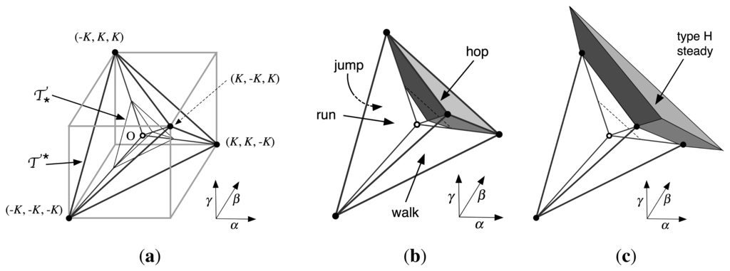
Figure 2.
Tetrahedral partition of connection-space. (a) The two tetrahedra (img), (img); (b) one of the four primary Hopf regions, in this case the hop gait. Base triangle left unshaded to show interior; (c) Extending the pyramid to define the corresponding steady-state regions, which extend to infinity in the direction indicated.
The four primary gait regions are relatively large when K is significantly greater than k. This is the case for reasonable values of the connection strengths and other parameters in the model, so the structure provides a robust way to select specific gait patterns.
Despite the nonlinear form of the equations, it turns out to be possible to derive much of the bifurcation behaviour analytically. The possibility of doing this stems from a pleasant property of a gain function commonly used in rate equations, combined with linearity of the argument of the gain function in the equations. The rate equations themselves have a symmetry group ℤ2 × ℤ2 of order 4, but the bifurcation behaviour is controlled by a larger group, the symmetries of a tetrahedron, of order 24. We describe how this group arises and why it determines many key aspects of the bifurcation behaviour. Ultimately, it is related to the eigenvalues of the connection matrix, which are closely related to the eigenvalues of the Jacobian for the rate equations, evaluated at a synchronous equilibrium.
Rate models in a network with the same symmetries are analysed in Diekman et al [25] in a model of binocular rivalry using Wilson networks (the “monkey/text” experiment). They assume a more general form of the gain function, but take β = 0, γ < 0 in Figure 1 because some connections in Wilson networks are always inhibitory, and the others are determined by a learning process.
We do not discuss the stability of the bifurcating states here, to avoid complicating an already lengthy paper. However, simulations suggest that all of the symmetry types of states that we describe can exist stably for some ranges of parameters.
Other types of dynamics can occur in this model, including apparent chaos, but the parameter regions concerned seem to be small. We do not discuss more exotic possibilities here. Curtu [26,27] and Curtu et al. [28] have analysed the bifurcations of a rate model for a network with two identical nodes (ℤ2 symmetry) in considerable detail. Even in this case there is a richer range of dynamic behaviour than equilibria and periodic states arising from local bifurcation. Note, however, that they assume that certain connections are inhibitory, so the corresponding connection strength is negative. This restriction implies in particular that there is a unique fully synchronous steady state for all parameter values under consideration. This is not the case when the signs are not restricted, as we show in Section 4.
This is the first in a projected series of papers. Others will discuss stability issues and investigate quadruped and hexapod gaits from a similar point of view. New features enter into the analysis, in part because the eigenvalues of the connection matrix can now be complex.
1.1. Structure of the Paper
In Section 2 we introduce gain functions, the connection matrix, and rate models. We establish some key properties of the family of gain functions used here. Section 3 describes the CPG network used to model biped gaits, sets up the corresponding rate equations, and discusses parameter symmetries used later to simplify the calculations. We also describe the four primary gaits hop, jump, run, and walk in the context of symmetric Hopf bifurcation, following Pinto and Golubitsky [21].
Section 4 analyses the fully synchronous steady states u of the rate equations, a preliminary step towards studying local bifurcations from such states. We show that these are described by a cusp catastrophe surface in the sense of Poston and Stewart [29] and Zeeman [30]. The geometry of this surface is used to show that the first local bifurcation as an input parameter I increases can be obtained from the corresponding bifurcation as u increases. This simplifies later calculations considerably and is central to the main theorem, a formal statement of Figure 2 that is stated in Section 7 and proved in Section 12.
Section 5 reviews basic existence results for local bifurcation (steady-state and Hopf) in symmetric ODEs. Section 6 summarises basic data for primary gaits: eigenvalues and eigenvectors of the connection matrix, symmetries of bifurcating branches for steady-state and Hopf bifurcation. We state the main theorem in Section 7.
Section 8 examines how the eigenvalues of the Jacobian evaluated at a fully synchronous equilibrium u relate to the eigenvalues of the connection matrix. It derives necessary and sufficient conditions for steady-state and Hopf bifurcations of given symmetry type to occur. These conditions are used to plot typical bifurcation curves for the primary gaits in Section 9.
Section 10 analyses which eigenvalue of the connection matrix is largest, as the connection strengths vary. The largest eigenvalue is closely associated with the first bifurcation to a state with the corresponding symmetry type. This principle is exploited in the proof of the main theorem, but first we discuss a symmetry group
 that acts on the set of eigenvalues of the connection matrix in Section 11. Here we prove that
also acts on the set of regions defining the first local bifurcation. The group
is not a symmetry group or parameter symmetry group of the rate equations in the sense of equivariance [18]. We also describe some general representation-theoretic reasons that explain this structure. We then prove the main theorem in Section 12.
that acts on the set of eigenvalues of the connection matrix in Section 11. Here we prove that
also acts on the set of regions defining the first local bifurcation. The group
is not a symmetry group or parameter symmetry group of the rate equations in the sense of equivariance [18]. We also describe some general representation-theoretic reasons that explain this structure. We then prove the main theorem in Section 12.We briefly discuss degeneracies in the connection strengths in Section 13. Most of these correspond to transitions between different first bifurcations, that is, to mode interactions. We observe that in some cases disjoint sets of nodes decouple, a feature of rate models that is non-generic in general symmetric dynamical systems. Finally, Section 14 shows simulations of the rate equations giving the four primary gaits.
2. Gain Functions and Rate Models
In a rate model, the state of node j is a vector
, where
is an activity variable that that corresponds to the rate at which the node fires and
is a fatigue variable. Nodes are coupled through a gain function  . This has a sigmoid shape, and ideally we take
(x) = 0 for x < 0. In practice, it is common to assume slightly less:
(x) ≪ 1 for x < 0. A node j is then considered to be quiescent if it is in equilibrium at a small value of
.
. This has a sigmoid shape, and ideally we take
(x) = 0 for x < 0. In practice, it is common to assume slightly less:
(x) ≪ 1 for x < 0. A node j is then considered to be quiescent if it is in equilibrium at a small value of
.
. This has a sigmoid shape, and ideally we take
(x) = 0 for x < 0. In practice, it is common to assume slightly less:
(x) ≪ 1 for x < 0. A node j is then considered to be quiescent if it is in equilibrium at a small value of
.The original choice of
in Wilson [31] was a ratio of two quadratic terms. However, throughout this paper we follow later practice and assume a gain function of sigmoid form
where a, b, c > 0. See Laing and Chow [32] and Shpiro et al. [33], who introduced such models in the context of binocular rivalry. With reasonable choices of a, b, c the value of
(x) is very small when x < 0. A standard choice in the literature is a = 0.8,b = 7.2, c = 0.9. For simplicity, we use a = 1, b = 8, c = 1 in simulations. In our analysis, a, b, c are arbitrary positive constants. We expect similar results to apply for any reasonable sigmoidal gain function, but proving this could be difficult, and some fine detail would be likely to change.
in Wilson [31] was a ratio of two quadratic terms. However, throughout this paper we follow later practice and assume a gain function of sigmoid form
(x) is very small when x < 0. A standard choice in the literature is a = 0.8,b = 7.2, c = 0.9. For simplicity, we use a = 1, b = 8, c = 1 in simulations. In our analysis, a, b, c are arbitrary positive constants. We expect similar results to apply for any reasonable sigmoidal gain function, but proving this could be difficult, and some fine detail would be likely to change.The function
has an inverse
 =
−1 given by
=
−1 given by
has an inverse
=
−1 given by
Let
 denote the derivative of
. There is an algebraic relation between
and
, which we exploit throughout this paper to obtain explicit formulas:
denote the derivative of
. There is an algebraic relation between
and
, which we exploit throughout this paper to obtain explicit formulas:
denote the derivative of
. There is an algebraic relation between
and
, which we exploit throughout this paper to obtain explicit formulas:
We also note that each member of this family of gain functions is symmetric about its inflection point. Specifically,
Indeed,
and tanh is odd.
We specify the rate model in terms of the connection matrix
where n is the number of nodes and αij ∈ ℝ is the strength of the connection from node j to node i (positive for excitation, negative for inhibition). Let g > 0 be a parameter that determines the strength of reduction of the activity variable by the fatigue variable. Assume that nodes have some kind of input, with the input to node i being Ii. The rate equations are:
for 1 ≤ i ≤ n. Since
we can write Equations (5) and (6) in the abbreviated form
where
,
,
and the obvious convention is used to apply
to a vector.
to a vector.The model Equations (5) and (6) is very similar to, and was partly motivated by, the concept of a Wilson network, modelling the brain's decision-making process when presented with conflicting, or potentially conflicting, inputs. See Wilson [34]. Wilson networks and generalisations have been used recently to model binocular rivalry and visual illusions [25,35–37]. The methods developed here also apply to some Wilson networks.
3. The CPG Network
Following Pinto and Golubitsky [21] we consider the 4-node network of Figure 1. Here, each leg corresponds to two nodes: one flexor and one extensor.
This network has symmetry group G = ℤ2 〈ρ〉 × ℤ2 〈τ〉 generated by
There are also parameter symmetries, of two kinds. First: any permutation of the four nodes produces the same network topology, but the connection strengths are permuted. For example (12) interchanges α and β, leaving γ fixed. Second: there is a parameter symmetry in which α, β, and γ are fixed but I changes, induced by the symmetry (4) of
. This leads to the following proposition, which is valid for rate equations on any homogeneous network, that is, one on which every node has the same number of input arrows of each type (connection strength). For example, in Figure 1 every node has one input arrow of type α, one of type β, and one of type γ. For rate models, it is convenient to employ a slightly more general condition: a network is homogeneous if and only if each row of the connection matrix A has the same sum r. That is,
Proposition 1 Suppose that a network  is homogeneous, with connection matrix A defining a rate model, so every row of A has the same sum r. Then the rate Equation (11) are invariant under the parameter symmetry η for which
and α, β, γ are fixed.
is homogeneous, with connection matrix A defining a rate model, so every row of A has the same sum r. Then the rate Equation (11) are invariant under the parameter symmetry η for which
and α, β, γ are fixed.
. This leads to the following proposition, which is valid for rate equations on any homogeneous network, that is, one on which every node has the same number of input arrows of each type (connection strength). For example, in Figure 1 every node has one input arrow of type α, one of type β, and one of type γ. For rate models, it is convenient to employ a slightly more general condition: a network is homogeneous if and only if each row of the connection matrix A has the same sum r. That is,
is homogeneous, with connection matrix A defining a rate model, so every row of A has the same sum r. Then the rate Equation (11) are invariant under the parameter symmetry η for whichWe employ the abbreviated notation of Equation (7), and scalars such as a are interpreted as [a, a,…, a]T. Let y = a − x, so that yE = a − xE and yH = a − xH. Then
and
These are the same equations as Equation (7) with the stated parameter changes.
Here the only parameter that changes is I. The connection strengths α, β, γ are unchanged; the waveform of the solution is turned upside down and shifted by a constant. This parameter symmetry explains why the numerical bifurcation diagram in Curtu [27] Figure 2A, showing how the activity variable xE (there denoted u1) depends on I, is symmetric under rotation through 180°.
For the network of Figure 1, the connection matrix is
This network is bidirectional (identical arrows point both ways) so A is symmetric. Therefore, A has real eigenvalues. We state them in Section 6.
To preserve symmetry, we take all inputs Ij to be equal, so that Ij = I for 1 ≤ j ≤ 4. We use I as bifurcation parameter and consider the connection strengths as subsidiary parameters; these are arbitrary, but held fixed as I varies. Explicit rate equations (written in a convenient order for later calculations, in which the activity variables and fatigue variables are collected together) are:
Here the parameters are:
Equation (11) have phase space
where
| α = | strength of diagonal connection |
| γ = | strength of medial connection |
| β = | strength of lateral connection |
| ε = | fast/slow dynamic timescale |
| g = | strength of reduction of activity variable by fatigue variable |
| I = | input |
The equations inherit the symmetry of the network, so they are equivariant under the action of G = ℤ2 × ℤ2 defined by
(It is usual to use the inverse h−1 to define a left action, but in this case every element of G is equal to its inverse.) The subspaces
,
are G-invariant subspaces with isomorphic G-actions.
Figure 3 shows the four phase patterns that occur generically in any ℤ2 × ℤ2-symmetric system at Hopf bifurcation, as classified in Pinto and Golubitsky [21]. We have abbreviated their “two-legged hop” and “two-legged jump” to “hop” and “jump”. Which pattern occurs is determined by the representation of ℤ2 × ℤ2 on the critical (purely imaginary) eigenspace [17,18,38]. See Section 5.
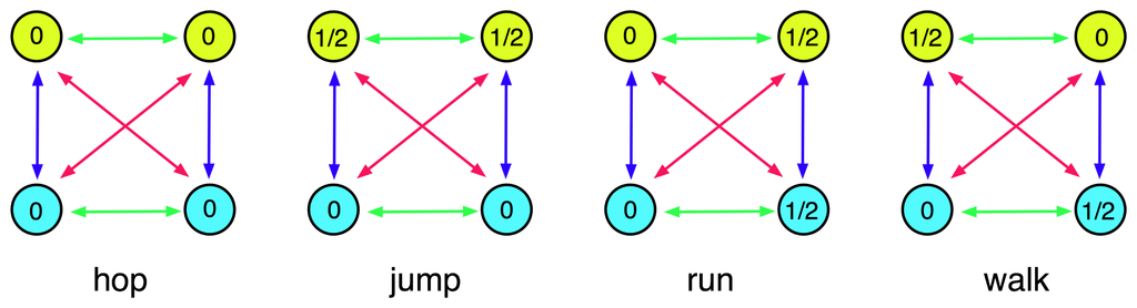
Figure 3.
Phase shift patterns for the four primary bipedal gaits. The numbers 0 and 1/2 indicate relative phases of the nodes.
This system can also undergo steady-state bifurcation, either symmetry-preserving or symmetry-breaking. This possibility is examined in Section 8.
4. Synchronous Steady States
As a preliminary step, we analyse fully synchronous steady states in the rate Equation (11) for the CPG network in Figure 1. That is, we determine conditions under which all nodes are in the same equilibrium state. Later we will consider local bifurcation from such states.
The main result generalises to any homogeneous network. When the network is homogeneous, the diagonal
is an invariant subspace for the dynamics. We call states in Δ fully synchronous.
Let the gain function be as in Equation (1), namely:
The function
is monotonic strictly increasing and always positive. There is a unique inflection point at
and the slope at that point is
. The curve is asymptotic to 0 as x → −∞ and to a as x → +∞. See Figure 4 for the case a = 1, b = 8, c = 1.
is monotonic strictly increasing and always positive. There is a unique inflection point at
and the slope at that point is
. The curve is asymptotic to 0 as x → −∞ and to a as x → +∞. See Figure 4 for the case a = 1, b = 8, c = 1.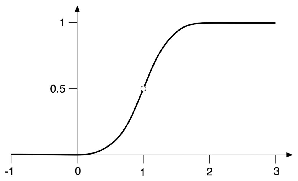
Figure 4.
Graph of gain function in the typical case a = 1, b = 8, c = 1. Here x runs horizontally and the vertical axis represents
(x).
(x).
We prove:
Theorem 1 Let be a homogeneous network whose connection matrix A has all row-sums equal to r. Let
be a homogeneous network whose connection matrix A has all row-sums equal to r. LetThen the fully synchronous equilibria u satisfy the equation
If σ ≤ 4/ab there is a unique solution for all I. If σ > 4/ab there exist IL, IU depending on σ for which there are three solutions when IL < I < Iu, and two solutions (one of multiplicity 2) when I = IL, IU.
The set of solutions to Equation (12) forms a cusp catastrophe surface in (σ, I, u)-space. Its bifurcation set in (σ, I)-space has the equation
where
Consider a fully synchronous equilibrium at which all nodes have
Equation (6) implies that
, so υ = u. Substituting in the equations for
we obtain the single equation
by Equation (8). Since σ = r − g we can rewrite this as
Apply
to deduce Equation (12).
to deduce Equation (12).The geometry of
, hence of
, implies that whenever σ ≤ c/2 there is a unique solution for all I. If σ > c/2 there exist IL, IU depending on σ for which there are three solutions when IL < I < IU , and two solutions (one of multiplicity 2) when I = IL, IU. See Figure 5 when a = 1, b = 8, c = 1.
, hence of
, implies that whenever σ ≤ c/2 there is a unique solution for all I. If σ > c/2 there exist IL, IU depending on σ for which there are three solutions when IL < I < IU , and two solutions (one of multiplicity 2) when I = IL, IU. See Figure 5 when a = 1, b = 8, c = 1.
Figure 5.
Solutions of Equation (12) when a=1, b = 8,c = 1. Here, u runs horizontally and the vertical axis represents the values of
(u)(curve) and I + σu (straight lines).
(u)(curve) and I + σu (straight lines).
The derivative of
is
is
The tangencies with lines of slope σ occur when
Solutions are real when σ < 0 or
. When σ < 0 both solutions are outside [0, 1]. When
both solutions are in [0, a], which we require.
Now substitute in Equation (15) to get
In Figure 6a we plot the curves IL, IU against σ. Not surprisingly, we recognise the bifurcation curve of a cusp catastrophe surface, Zeeman [30], Poston and Stewart [29]. Figure 6b shows this surface. There are three solutions to Equation (12), that is, three fully symmetric equilibria, when (σ, I) lies inside the cusp; a unique solution when (σ, I) lies outside the cusp; two solutions (one with multiplicity 2) when (σ, I) lies on the curves except at the cusp point; and one solution (with multiplicity 3) when (σ, I) lies at the cusp point.
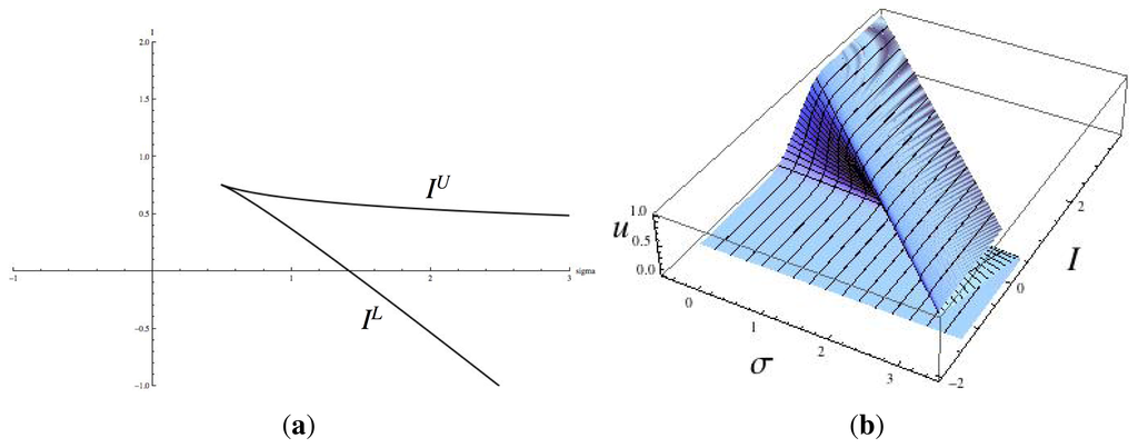
Figure 6.
(a) The curves IU , IL plotted against σ. Parameter values in the gain function are a = 1, b = 8, c = 1; (b) the cusp catastrophe surface in (σ, I, u)-space.
If we fix a value of σ and use I as bifurcation parameter (one reasonable choice) then the bifurcation diagram is the usual S-shaped curve when
: this can be seen in constant-I cross-sections of Figure 6b, especially at the right of the figure. With quasistatic variation of the bifucation parameter I, the first steady state bifurcation occurs on crossing the upper branch IU of the cusp curve, which corresponds to u−. As we show later, there is always a Hopf bifurcation before that point. However, that does not rule out a synchrony-breaking steady-state bifurcation occurring before the Hopf bifurcation. We consider this possibility in Section 12 and show that it does not occur.
Remark 1 Curtu [26,27] study a rate model on a network with two identical nodes, and Theorem 1 applies to this network. However, in those papers there is a unique fully synchronous equilibrium for all I. The reason for this apparent discrepancy is that those papers assume an inhibitory connection, so σ < 0. Therefore, σ < c/2 since c > 0.
The Cusp Catastrophe. The geometry of the cusp catastrophe surface makes it relatively straightforward to understand how the first bifurcation from a synchronous equilibrium (as I varies quasistatically) depends on the connection strengths. See Zeeman [30] and Poston and Stewart [29] for further discussion in the context of the canonical cusp catastrophe. More precisely, the cusp geometry motivates the following procedure.
For each (α, β, γ) recall that σ = α+ β +γ − g. Define a map
Geometrically, the image of ξσ is the constant-σ section of the cusp surface
 . Define a projection
. Define a projection
This maps
to the parameter space (σ, I), and its singularities determine the fold lines and cusp point. The bifurcation varieties for local bifurcation are the images under π ○ ξσ of the corresponding varieties in (σ, u)-space. Therefore, saddle-node (fold) bifurcations in the fully synchronous state u, which correspond to tangencies in Figure 5, are given by Equation (15), so that
along with Equation (16). The next lemma shows that we can invert ξσ on suitable domains to rewrite this as
Lemma 1 For given connection strengths (α, β,γ), let σ = α + β + γ − g. Then
to the parameter space (σ, I), and its singularities determine the fold lines and cusp point. The bifurcation varieties for local bifurcation are the images under π ○ ξσ of the corresponding varieties in (σ, u)-space. Therefore, saddle-node (fold) bifurcations in the fully synchronous state u, which correspond to tangencies in Figure 5, are given by Equation (15), so that
- If then ξσ : ℝ → (0, a; is a monotonic strictly increasing diffeomorphism.
- If then ξσ : ℝ → (0, a; is a monotonic strictly increasing homeomorphism.
- If and ξσ : (0,u−) → (−∞,IU) is a monotonic strictly increasing homeomorphism. It is a diffeomorphism when u < u−.
The proof is a restatement of the analysis in Theorem 1 and Equation (17).
We can therefore use u as bifurcation parameter in place of I when considering the first bifurcation, provided we consider quasistatic changes as I increases from stable equilibrium. That is, I remains in equilibrium and varies continuously while this is possible. By Lemma 1 this first ceases to be possible only when
and I reaches IU, the saddle-node bifurcation on the lower layer of the cusp surface
. We therefore have:
. We therefore have:Proposition 2 For any given α, β, γ the first local bifurcation as I increases quasistatically corresponds to the first local bifurcation as u increases.
By Lemma 1, if
then all local bifurcations occur in the same order using either I or u as bifurcation parameter. If
then all local bifurcations occur in the same order when I ≤ IU , provided we consider quasistatic variation. But IU is itself a bifurcation point—here a saddle-node.
This proposition is decisive because the geometry of the bifurcation curves is much simpler in terms of u than it is using I.
Local bifurcations that are not the first can be converted from u to I using Equation (17) no matter what the value of σ may be. But when ξσ is not invertible, the order gets mixed up. See the crossings in some of the Hopf bifurcation curves in Figures 7, 8, 9, 10, 11, 12, 13 and 14 below.

Figure 7.
Hopf curves. Parameter values are: a = 1, b = 8, c = 1; g = 1.8, ε = 0.67, α = 0.4, β = 0.7. Hop = red, jump = green, run = magenta, walk = blue, cusp = black.

Figure 8.
Hopf curves. Parameter values are: a = 1, b = 8, c = 1; g = 1.8, ε = 0.67, α = 0.4, β = −0.7. Hop = red, jump = green, run = magenta, walk = blue, cusp = black.

Figure 9.
Hopf curves. Parameter values are: a = 1, b = 8, c = 1; g = 1.8, ε = 0.67, α = −0.4, β = 0.7. Hop = red, jump = green, run = magenta, walk = blue, cusp = black.
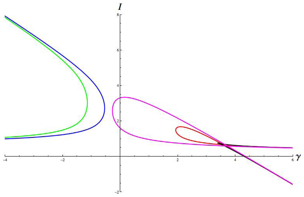
Figure 10.
Hopf curves. Parameter values are: a = 1, b = 8, c = 1; g = 1.8, ε = 0.67, α = −0.4, β = −0.7. Hop = red, jump = green, run = magenta, walk = blue, cusp = black.

Figure 11.
Hopf curves. Parameter values are: a = 1, b = 8, c = 1; g = 1.8, ε = 0.67, α = 1, β = 0.7. Hop = red, jump = green, run = magenta, walk = blue, cusp = black.
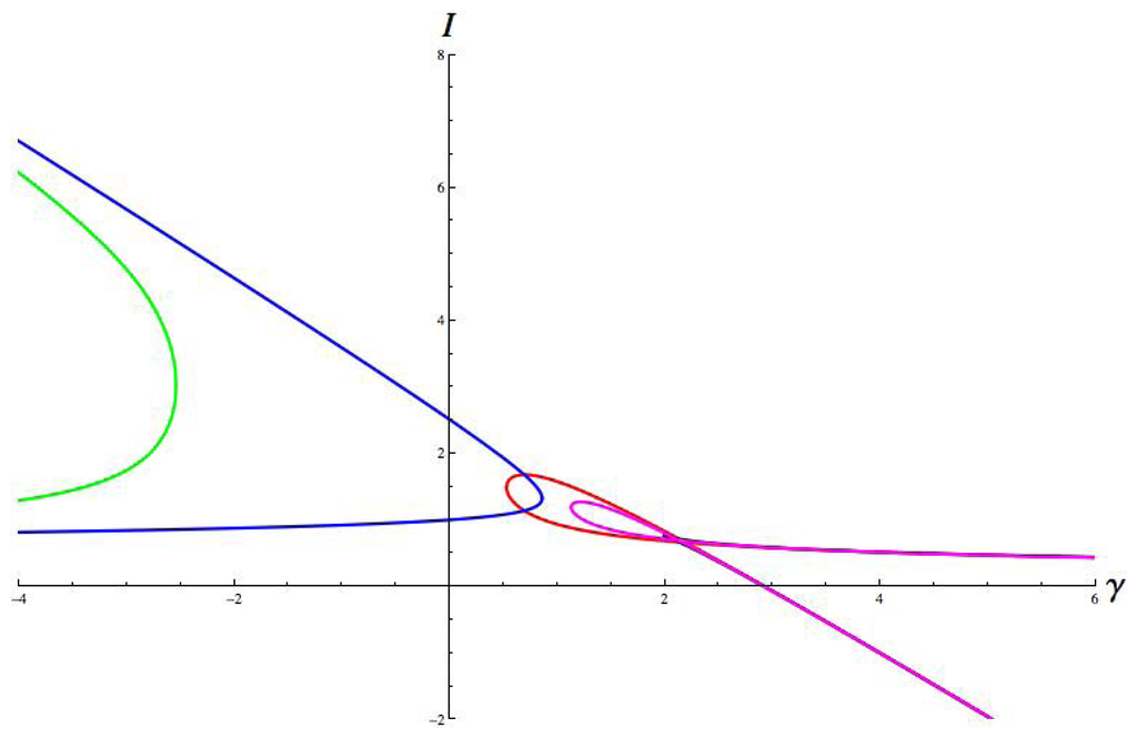
Figure 12.
Hopf curves. Parameter values are: a = 1, b = 8, c = 1; g = 1.8, ε = 0.67, α = 1,β = −0.7. Hop = red, jump = green, run = magenta, walk = blue, cusp = black.
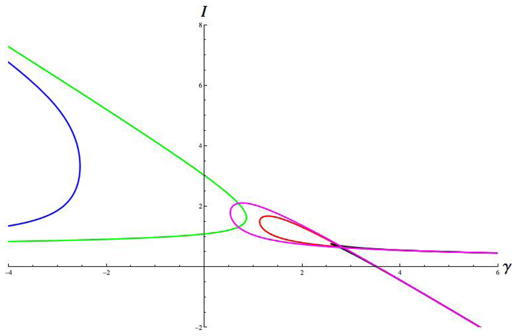
Figure 13.
Hopf curves. Parameter values are: a = 1, b = 8, c = 1; g = 1.8, ε = 0.67, α = −1, β = 0.7. Hop = red, jump = green, run = magenta, walk = blue, cusp = black.

Figure 14.
Hopf curves. Parameter values are: a = 1, b = 8, c = 1; g = 1.8, ε = 0.67, α =− 1, β = −0.7. Hop = red, jump = green, run = magenta, walk = blue, cusp = black.
5. Review of Symmetric Steady-State and Hopf Bifurcation
Our main goal is to analyse the time-periodic gait patterns generated by the four-cell CPG of Figure 1. The symmetries of the primary gaits are spatio-temporal patterns, combining permutations of the cells with phase shifts. We assume that these patterns arise through symmetry-breaking Hopf bifurcation from a fully synchronous state, and use the Equivariant Hopf Theorem [17,18,38] to determine the corresponding bifurcation varieties: the subsets of parameter space at which bifurcations occur. The relevant parameters are I, which we take to be the main bifurcation parameter and the connection strengths α, β, γ. We assume that a, b, c, g, ε are fixed and positive.
However, steady-state bifurcations also occur in the rate equations. These correspond to various “stand” gaits, where the animal is motionless, which may not be of great interest. (However, there is a difference between passive standing and “getting ready” to initiate a periodic gait, which is one way to interpret these symmetry-breaking equilibria.) At any rate, the analysis has to take them into account. We discussed the bifurcation of synchronous (that is, symmetry-preserving) steady states in Section 5. Here we review general theorems about symmetry-breaking local bifurcations. We state the Equivariant Branching Lemma for the existence of steady-state bifurcations with specified symmetry types. We also summarise the Equivariant Hopf Theorem and specify our notational conventions. This helps to avoid potential confusion in the later analysis, because several different conventions exist in the literature. We follow [17,18,38], with some minor changes. We apply these results in Section 8.
Let G be a group (technically, a compact Lie group, which includes all finite groups) acting linearly on ℝn. Denote the action of g ∈ G on x ∈ ℝn by gx. Consider a G-equivariant ODE
where f : ℝn × ℝ → ℝn is smooth. Here x represents the state of the system and λ is a bifurcation parameter. The equivariance condition is
It follows that if x(t) is a solution of a G-equivariant ODE and g ∈ G, then gx(t) is also a solution. We do not consider such solutions to be significantly different from x(t), and by abuse of terminology call them conjugate solutions to x(t). The name arises because their symmetry groups are conjugate in G.
Assume that as λ varies near λ0 there is a path of equilibria {(x(λ), λ) : λ ∈ ℝ}. Local bifurcations (either steady-state or Hopf; occur at points (x0, λ0) for which the Jacobian
has at least one eigenvalue on the imaginary axis. Here the steady state loses stability. A zero eigenvalue corresponds to steady-state bifurcation, and a complex conjugate pair of purely imaginary eigenvalues corresponds to Hopf bifurcation to a time-periodic state.
5.1. Symmetric Steady-State Bifurcation
Steady-state bifurcation in the presence of symmetry is governed by the Equivariant Branching Lemma of Cicogna [39] and Vanderbauwhede [40,41]. To state it we need some group-theoretic concepts.
The isotropy subgroup of x ∈isin;ℝn is
and the isotropy subgroup of a solution x(t) is
Conversely, if Σ is a subgroup of G then the fixed-point subspace of Σ is
This space is invariant under the normaliser Ng(Σ). Since Σ acts trivially, the effective action is that of Ng(Σ)/Σ.
If G is a compact Lie group, and in particular if G is finite, which is the case for gaits, then G ×
 1 is a compact Lie group. Finite-dimensional real linear representations of compact Lie groups occur in three classes, distinguished by the space of commuting linear maps. By Schur's Lemma this is a division algebra over ℝ, hence is isomorphic to one of ℝ, ℂ, and the quaternions (x0210D;. If this algebra is (x0211D; we call the representation absolutely irreducible. See Adams [42] 3.22.
1 is a compact Lie group. Finite-dimensional real linear representations of compact Lie groups occur in three classes, distinguished by the space of commuting linear maps. By Schur's Lemma this is a division algebra over ℝ, hence is isomorphic to one of ℝ, ℂ, and the quaternions (x0210D;. If this algebra is (x0211D; we call the representation absolutely irreducible. See Adams [42] 3.22.Proposition 3.2 of Chapter XIII of [18] states:
Proposition 3 Let f be a G-equivariant bifurcation problem (19), and suppose that along a branch of steady states (x(λ),λ) the Jacobian Df|(x0,λ0) has a zero eigenvalue, where x0 = x(λ0). Let E0 be the corresponding real generalised eigenspace. Then generically E0 is absolutely irreducible under the action of G.
A proof of the Equivariant Branching Lemma of Cicogna [39] and Vanderbauwhede [40,41] is given in Proposition 3.3 of Chapter XIII of [18], which states:
Lemma 2 Consider a G-equivariant bifurcation problem (19) such that Df|(x0,x0) has a zero eigenvalue for which E0 is absolutely irreducible and the eigenvalue passes through zero with nonzero speed. Let Σ be an isotropy subgroup of G acting on E0 for which
Then there exists a unique branch of steady-state solutions to Equation (19), bifurcating from (x0, λ0), with isotropy group Σ.
Note that it is the action of Σ on E0 that is required to have a 1-dimensional fixed-point space, not the action on ℝn.
5.2. Symmetric Hopf Bifurcation
The Equivariant Hopf Theorem provides information about the spatio-temporal symmetries of bifurcating branches of periodic states. It also applies in circumstances where the classical Hopf bifurcation theorem does not, namely multiple eigenvalues caused by symmetry.
Let
2π,
be the loop spaces of continuous and once-differentiable 2π-periodic maps ℝ → ℝn. These are Banach spaces. Define the circle group
2π,
be the loop spaces of continuous and once-differentiable 2π-periodic maps ℝ → ℝn. These are Banach spaces. Define the circle groupThen G ×
1 acts on
2π and
by
1 acts on
2π and
by
A map υ ∈
2π or
is fixed by (g, θ) if and only if
or equivalently
2π or
is fixed by (g, θ) if and only if
So, transformation of υ(s) by g has the same effect as a phase shift θ. The spatio-temporal isotropy group of υ is the set of all (g, θ) ∈ G × 1 for which Equation (20) is valid. A representation W of G is said to be G-simple if either
1 for which Equation (20) is valid. A representation W of G is said to be G-simple if either
- (1)
- W ≅ V ⊕ V where V is absolutely irreducible.
- (2)
- W is irreducible of type ℂ or ℍ.
Proposition 1.4 of [18] states:
Proposition 4 Let f be a G-equivariant bifurcation problem (19), and suppose that along a branch of steady states (x(λ), λ) the Jacobian Df|(x0,λ0) has purely imaginary eigenvalues ±iω, where x0 = x(λ0) and ω ≠ 0. Let Eiω be the corresponding real generalised eigenspace. Then generically Eiω is G-simple.
It is clear that Eiω is always G-invariant. In the generic case it also supports a natural
1-action. Define the restricted Jacobian
1-action. Define the restricted JacobianWe can define an action of
1 on Eiω by
where we use |ω| to fix the orientation, an issue that becomes important for quadruped gaits to distinguish gaits like buck and walk from their reverses.
1 on Eiω by
By equivariance, J commutes with any g ∈ G. So G × 1 acts on Eiω by
1 acts on Eiω by
We say that the eigenvalues ±iω cross the imaginary axis with nonzero speed if there is a family of eigenvalues ρ(λ) ± σ(λ)i of D|f(x,λ(x)) for λ near λ0, such that
The Equivariant Hopf Theorem of [17,38] is proved in Theorem 4.1 of Chapter XVI of [18], and states:
Theorem 2 Consider a G-equivariant bifurcation problem (19) such that Df|(x0,λ0) has apair of purely imaginary eigenvalues ±iω for which Eiω is G-simple and the eigenvalues cross the imaginary axis with nonzero speed. Let Σ be an isotropy subgroup of G×
1 acting on Eiω for which
1 acting on Eiω for which
Then there exists a unique branch of small-amplitude time-periodic solutions to Equation (19), bifurcating from (x0, λ0), with period near
, having spatio-temporal symmetry group Σ in loop space.
Notice that we use the linearised action of J to define the circle group action on the critical eigenspace, for which dimℝ Fix(Σ) is computed, and infer the existence of a periodic solution of the full nonlinear equation with the same group Σ as its spatio-temporal symmetry group in loop space. So the symmetries are exact, not linearised approximations.
In the generic case where the critical eigenspace is G-simple, the spatio-temporal symmetry groups can be characterised as twisted subgroups
where
is a group homomorphism. See Proposition 7.2 page 300 of [18].
The group H consists of all setwise symmetries of the trajectory through υ. The kernel K = ker ϕ is the subgroup of all pointwise symmetries of that trajectory. The pair (H, K) provides a useful classification of the time-periodic solutions, and is characterised by the H/K Theorem of Buono and Golubitsky [16]. However, there can exist different (that is, non-conjugate) solutions with the same pair (H, K). Examples in gaits are the walk and reverse walk. This distinction arises in particular for analogous models of quadruped and hexapod locomotor CPGs.
When G is abelian (as it is for ℤ2 × ℤ2) a G-simple critical eigenspace generically corresponds to a simple eigenvalue, so the classical Hopf bifurcation theorem applies. In particular, the bifurcating branch is locally unique. However, the Equivariant Hopf Theorem is a stronger result because the spatio-temporal isotropy subgroup provides additional information about the symmetries along the bifurcating branch. Similar remarks apply to steady-state bifurcation.
6. Data for Primary Gaits
Bifurcation depends on the eigenvalues of the Jacobian, and we will see that these are closely related to the eigenvalues of the connection matrix A. The eigenvectors and eigenvalues of A are given in Buono [14], Buono and Golubitsky [16], and Golubitsky et al. [19,20]. Using T to denote column vectors, a basis adapted to the four irreducible representations of ℤ2 × ℤ2 on ℝ4 is:
By equivariance or direct verification, these are the eigenvectors of A. The corresponding eigenvalues are:
where we use H, J, R, W to denote the four gait patterns hop, jump, run, walk respectively.
The next proposition is trivial but important. Equalities between eigenvalues of A correspond to degeneracies in the bifurcations or the dynamics: see Section 13.
Proposition 5 The eigenvalues of A are distinct unless
As well as A having equal eigenvalues, there are other conditions that cause degeneracies in the bifurcations. We list them here:
Definition 1 A triple of connection strengths (α, β, γ) is degenerate if any of the following conditions is satisfied for some patterns P, Q:
The first of these conditions is equivalent to Equation (22). We consider the second in Section 13.
Pinto and Golubitsky [21] list the spatio-temporal isotropy subgroups of the primary gaits obtained by Hopf bifurcation in this ℤ2 × ℤ2-symmetric network. We reproduce that table in the notation of this paper as Table 1, using Σ in place of their K to denote the spatial (that is, pointwise) isotropy subgroup. For all primary gaits, the setwise isotropy subgroup H is ℤ2 × ℤ2. Since the group is abelian, this is also the normaliser of Fix(Σ). Recall that
= ℝ/2πℤ so π is half the period.
= ℝ/2πℤ so π is half the period.
Table 1.
Spatio-temporal isotropy subgroups of the primary gaits.
The same four isotropy groups determine the possible actions on a critical eigenspace E0 for steady-state bifurcation, in the generic case when this space has dimension 1. We say that such a steady-state bifurcation is of type P if the isotropy subgroup is that of the primary gait P (= H, J, R, or W). Steady-state bifurcation of type H is symmetry-preserving; the other three are symmetry-breaking.
7. Main Theorem
We can now state the main theorem of this paper. It provides a complete characterisation of the regions of parameter space for which the first bifurcation is of a given type, as illustrated in Figure 2. Most of the remainder of the paper will provide a proof.
Theorem 3 Let
Assume that k < K, that is, ε < abg/4. Suppose that μP ≠ k, K and none of the conditions (22) holds. Then the first local bifurcation (or its absence) is given by Table 2.
Table 2.
Necessary and sufficient conditions for each type of first bifurcation when no degeneracy condition holds.
We develop the proof of this theorem in stages in the following sections.
Remark 2 The assumption that ε < abg/4 is natural because it is usual to assume that ε ≪ 1, leading to fast/slow dynamics. If ε > abg/4, no parameter values lead to Hopf bifurcation.
8. Local Bifurcation Analysis
We now derive conditions for local bifurcations of given symmetry type (that is, spatial isotropy subgroup) H, J, R, or W. Subject to technical genericity conditions, a local bifurcation occurs when the Jacobian Ju at a fully synchronous equilibrium u has an eigenvalue on the imaginary axis. If it is zero, we get a steady-state bifurcation and the bifurcating branch consists of equilibria; if it is purely imaginary, we get a Hopf bifurcation and the branch consists of periodic states.
8.1. Eigenvalues of the Jacobian
It turns out that for any rate model with n nodes, there is a strong connection between the eigenvalues and eigenvectors of the Jacobian Ju at a fully synchronous equilibrium u, and those of the connection matrix A. We therefore begin with a general theorem characterising the relation between eigenvalues and eigenvectors of Ju and those of A.
Write the variables in the order
,…,
;
,…,
. From Equations (5) and (6) the Jacobian at a fully synchronous equilibrium u takes the block form
where
Theorem 4 Let υ be an eigenvector of A with eigenvalue μ. Then [(λ + 1)υ, υ]T is an eigenvector of Ju with eigenvalue λ if and only if
Moreover, every eigenvector is of this form.
Let w, υ ∈ ℝn. Then [w, υ]T is an eigenvector of Ju with eigenvalue λ if and only if
This suggests taking υ to be an eigenvector of A, say Aυ = μυ. We then get
Therefore, if Equation (26) holds we obtain an eigenvector of Ju. Solving Equation (26) yields:
which we can rewrite as
Finally, we must show that every eigenvector is of this form. If an arbitrary [w, υ]T is an eigenvector of Ju with eigenvalue λ, conditions Equations (27) and (28) are valid. By Equation (28) w = (λ + 1)υ. Substituting for w in Equation (27) now proves that υ is an eigenvector of A, unless λ + 1 = 0; that is, λ = −1. We claim that −1 is not an eigenvalue of Ju. If it is, Equation (28) implies that w = 0, and Equation (27) reduces to gΓυ = 0, implying that gΓ = 0. But the parameter g in Equation (5) is greater than 0, and Equation (25) implies that Γ > 0, a contradiction.
Remark 3 Generically, the quadratic Equation (26) has two distinct solutions. The solutions coincide if
We discuss this condition in Theorem 10, and prove that at any local bifurcation it holds only when μ = K. This is a standard degeneracy condition for μ and corresponds to the transition from Hopf to steady-state for a given symmetry type P, where μ = μP. Generically in the connection strengths it does not occur.
Corollary 1 For any α,β,γ, and sufficiently small I, the unique synchronous steady state u is linearly stable.
Let I →− ∞. Then Γ → 0, so (26) becomes
so all eigenvalues λ at u are negative for sufficiently small I.
In fact, the subsequent analysis of local bifurcations shows that u is linearly stable when I ≤ 0, indeed for larger I, provided we consider quasistatic variation of I from −∞ and ignore non-local bifurcations (such as jumps to the upper sheet of the cusp catastrophe surface).
Remark 4 The Hopf bifurcation curves in Figures 7, 8, 9, 10, 11, 12, 13 and 14 below, corresponding to hop and run, have segments with negative I. This does not contradict stability of the steady state for sufficiently small I because these segments are not relevant when I varies quasistatically.
Corollary 2 If (α, β, γ) is not degenerate in the sense of Definition 1, the Jacobian Ju is semisimple (diagonalisable) over ℂ.
Generically in connection-strengths, the eigenvalues μP are distinct as P ranges over the four patterns.
Generically in u, the above construction yields two distinct λ for each μ. The form [(λ + 1)υ, υ]T of the eigenvectors implies that distinct patterns P, Q lead to distinct eigenvectors μp,μq, even if the associated eigenvalues are equal. This is the case even when there are degeneracies in the connection strengths (α,β,γ).
Corollary 2 shows that in the local bifurcation analysis for nondegenerate connection strengths, Theorem 4 determines all eigenvalues and eigenvectors of Ju.
8.2. Conditions for Steady-State Bifurcation
We seek conditions for the corresponding λ eigenvalues to be purely imaginary. Here we work with a general network, making the assumption that μ is real. In particular, this is the case for all eigenvalues of A when the network is the one in Figure 1.
Theorem 5 Suppose that μ is real. Then the eigenvalue λ (evaluated at the synchronous equilibrium u) is zero if and only if the following equivalent conditions hold:
This leads to Equation (32), and also implies that
8.3. Conditions for Hopf Bifurcation
We seek conditions for the corresponding eigenvalues λ to be purely imaginary. Again, we work with a general network, but now we assume that μ is real. A similar but more complicated result for complex μ, can be proved, but we omit it here because it is not required.
Theorem 6 Suppose that μ is real. Then the eigenvalue λ (evaluated at the synchronous equilibrium u) is purely imaginary if and only if
Substitute in Equation (39) to get
bearing in mind that ε > 0. Therefore, Γ > ε/g, bearing in mind that g > 0. Substitute in Equation (40) to get
as claimed.
In the simulations of Section 14,
is approximately 4.5.
We can now derive a necessary condition for Hopf bifurcation from a synchronous equilibrium, for the primary gaits.
Theorem 7 Let μP be the eigenvalue for the primary gait P, where P = H, J, R, or W. Then the necessary condition (38) for Hopf bifurcation to gait P is valid if and only if
where
Also
(the first by definition, the second by Theorem 6). Therefore
by Equation (3). That is,
This has solutions
and then
as claimed.
Since A generically has four linearly independent eigenvectors (by equivariance under ℤ2 × ℤ2) we obtain 8 eigenvectors by this method, except when there is a solution of multiplicity 2 to Equation (26), which is non-generic as discussed in Theorem 10 below.
9. Plots of Hopf Bifurcation Curves
We now use Equations (41) and (42) to plot the Hopf bifurcation curves in (γ, I)-space for selected choices of α, β. More precisely, we plot curves given by the necessary condition (38) for Hopf bifurcation. For the moment we ignore the inequality (39), which leads to sufficient conditions by guaranteeing that the eigenvalue μ is imaginary.
These plots illustrate the main possibilities and motivate the subsequent analysis.
Note that μ is real for all four gaits: it is the corresponding eigenvalue λ of J that is imaginary. In simulations, we choose to fix α, β and plot the curve of I against γ. Figures 7, 8, 9, 10, 11, 12, 13 and 14 show such plots for representative choices of α, β.
These plots share some general features. The curves for jump and walk extend towards γ = −∞, while those for hop, run, and the fold curve of the cusp extend towards γ = +∞. This feature is a consequence of the sign of γ in μP and in σ. The hop and run curves fold over with a self-intersection. This is a consequence of the map ξσ in Equation (18). The upper branch of the curve corresponds to the lower sheet of the cusp surface, and the lower branch of the curve corresponds to the upper sheet of the cusp surface: this follows since IU is defined by u− and IL is defined by u+ in Equation (13).
In some of these plots, there is no Hopf bifurcation for some parameter values. For example, this is the case for Figures 7, 8, 9 and 10, where there is a gap (corresponding to some interval of values of γ) between the bifurcation curves for jump/walk and hop/run. However, other plots, such as Figures 11, 12, 13 and 14, do not have this gap. In Section 12 we show that the gaps correspond to connection strengths for which there is no local bifurcation from the branch of symmetric equilibria as I increases. (This is not yet obvious because there might be a symmetry-breaking steady-state bifurcation in this range.)
10. Dominant Eigenvalues
Local bifurcation from a fully synchronous state u is determined by the eigenvalues of the Jacobian Ju. However, Equation (26) implies that the overall “skeleton” for the partition of (α, β, γ)-space, according to the type of the first bifurcation (relative to I, or equivalently to u), is determined by which of the four eigenvalues μP of the connection matrix A is largest. We discuss this issue first.
Theorem 8 Assume that the degeneracy conditions (22) do not hold. Then the largest eigenvalue of A is:
This follows directly from Equation (21). For example, μH > μJ if and only if α+β+γ > −α+β−γ, that is, α + γ > 0. Five similar comparisons establish the stated conditions.
Remark 5 If any of the degeneracy conditions (22) is valid, two or more eigenvalues become equal.
The conditions (44) partition ℝ3 = {(α,β,γ)} into four open regions. Their closure is ℝ3 and the complement of their union comprises values of (α,β,γ) satisfying at least one of the degeneracy conditions (22).
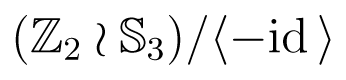
It is convenient to draw these regions by considering constant-γ sections of (α,β,γ)-space, since these are planes. For fixed γ the inequalities (44) let us plot the regions of (α, β) values corresponding to the four gaits. Figure 15 shows these regions for γ > 0, γ < 0.

Figure 15.
Regions of (α, β) values corresponding to the four gaits. (a) γ > 0; (b) γ < 0.
In three dimensions the structure of this partition is tetrahedral, and we can describe it in terms of the tetrahedron
 with vertices at
with vertices at
For any constant c the four planes μP = c, for P = H, J, R, W, are parallel to the four faces of
. In fact, since the vertices of c are (±c, ±c, ±c) with 1 or 3 minus signs, they contain the faces of c . Define the face FP of
corresponding to gait P as follows:
. In fact, since the vertices of c are (±c, ±c, ±c) with 1 or 3 minus signs, they contain the faces of c . Define the face FP of
corresponding to gait P as follows:
- (1)
- FH is the face with vertices (−1, 1, 1), (1, −1, 1), (1, 1, −1)
- (2)
- FJ is the face with vertices (−1, 1, 1), (1, −1, 1), (−1, −1, −1)
- (3)
- FR is the face with vertices (−1, 1, 1), (1, 1, −1), (−1, −1, −1)
- (4)
- FW is the face with vertices (1, −1, 1), (1, 1, −1), (−1, −1, −1)
Routine calculations, or an examination of Figure 15, show that the inequalities (44) partition (α, β, γ)-space into four connected regions:
Theorem 9 For each gait pattern P, the region RP of (α, β, γ) -space in which μP is larger than the other three eigenvalues of A is the positive cone
In more detail, RP is the interior of an infinite triangular pyramid obtained by extending to infinity the pyramid with base FP and vertex the origin. These regions are related by rigid motions, corresponding to symmetries of
. Figure 2b illustrates the three-dimensional geometry involved.
. Figure 2b illustrates the three-dimensional geometry involved.A direct derivation in three dimensions is sketched in Remark 7 below.
11. Tetrahedral Structure
As Figure 15 suggests, the entire problem has an elegant tetrahedral structure, which arises from the expressions for the eigenvalues of A and the linear form of the argument of
in Equation (5). Indeed, there is a general representation-theoretic reason for it, which we explain at the end of this section. The tetrahedral symmetry involved is richer than the symmetry group ℤ2 × ℤ2 of the CPG network, and also richer than the parameter symmetries
3 acting on α, β, γ. It simplifies the proof of Theorem 3.
in Equation (5). Indeed, there is a general representation-theoretic reason for it, which we explain at the end of this section. The tetrahedral symmetry involved is richer than the symmetry group ℤ2 × ℤ2 of the CPG network, and also richer than the parameter symmetries
3 acting on α, β, γ. It simplifies the proof of Theorem 3.The CPG
of Figure 1 can be represented as a tetrahedron, with the nodes corresponding to vertices and the arrows to edges. In fact, Figure 1 can be seen as the projection of a tetrahedron in which nodes 1 and 4 lie in a different horizontal plane from, nodes 2 and 3. Arrows of a given type (α, β, or γ) correspond to pairs of opposite edges—not having a common vertex.
of Figure 1 can be represented as a tetrahedron, with the nodes corresponding to vertices and the arrows to edges. In fact, Figure 1 can be seen as the projection of a tetrahedron in which nodes 1 and 4 lie in a different horizontal plane from, nodes 2 and 3. Arrows of a given type (α, β, or γ) correspond to pairs of opposite edges—not having a common vertex.The symmetry group
4 of the tetrahedron acts on the four vertices by permuting them. We will see that this action of the tetrahedral group does not fully explain the tetrahedral structure of the first bifurcations, although it goes part way. Instead, we require a subtler (though related) action. We first discuss the above action.
4 of the tetrahedron acts on the four vertices by permuting them. We will see that this action of the tetrahedral group does not fully explain the tetrahedral structure of the first bifurcations, although it goes part way. Instead, we require a subtler (though related) action. We first discuss the above action.The action of
4 on nodes induces a permutation of the three pairs of opposite edges, that is, of the symbols (α, β, γ). This arises via the standard homomorphism
with kernel the Klein four-group
 ≅ ℤ2 × ℤ2. See for example Rotman [43] page 42. Here
comprises the parameter symmetries that fix the parameters, that is, the symmetry group ℤ2 × ℤ2 of
.
≅ ℤ2 × ℤ2. See for example Rotman [43] page 42. Here
comprises the parameter symmetries that fix the parameters, that is, the symmetry group ℤ2 × ℤ2 of
.
4 on nodes induces a permutation of the three pairs of opposite edges, that is, of the symbols (α, β, γ). This arises via the standard homomorphism
≅ ℤ2 × ℤ2. See for example Rotman [43] page 42. Here
comprises the parameter symmetries that fix the parameters, that is, the symmetry group ℤ2 × ℤ2 of
.There is an induced action of
4, also with kernel
, and
4 acts as rigid motions of
4, also with kernel
, and
4 acts as rigid motions of
Since
4 acts by parameter symmetries, the partition of ℝ3 into regions in Figures 15, 16 and 17 are preserved. This action preserves the face of the large tetrahedron that forms the base of the “hop” region, and permutes the other three regions.
4 acts by parameter symmetries, the partition of ℝ3 into regions in Figures 15, 16 and 17 are preserved. This action preserves the face of the large tetrahedron that forms the base of the “hop” region, and permutes the other three regions.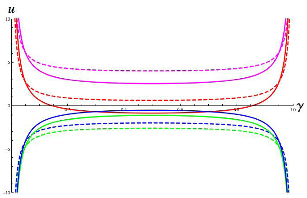
Figure 16.
Typical set of bifurcation curves for fixed (α, β), showing u against γ. Hop = red, jump = green, run = magenta, walk = blue. Solid lines = Hopf, dashed lines = steady. Parameter values: a = 1, b = 8, c= 1; g = 1.8, ε = 0.67, α = 1, β = 0.7.

Figure 17.
Regions of (α, β) values corresponding to the four gaits when the “gap” region is excluded. (a) γ > 0; (b) γ < 0. Inner rectangle is empty when γ > k; outer rectangle is empty when γ > K.
These parameter symmetries explain the
3 symmetry of Figure 15, but not the tetrahedral symmetry. To see how this arises, we consider a different group acting on the set of linear forms ±α ± β ± γ that include the four eigenvalues of A. This is the wreath product
 of order 48, Hall [44]. Here the base group ℤ2 × ℤ2 × ℤ2 changes the signs of α, β, γ, and
3 permutes them. Geometrically,
is the symmetry group of rigid motions of the cube with vertices (±1, ±1, ±1).
of order 48, Hall [44]. Here the base group ℤ2 × ℤ2 × ℤ2 changes the signs of α, β, γ, and
3 permutes them. Geometrically,
is the symmetry group of rigid motions of the cube with vertices (±1, ±1, ±1).
3 symmetry of Figure 15, but not the tetrahedral symmetry. To see how this arises, we consider a different group acting on the set of linear forms ±α ± β ± γ that include the four eigenvalues of A. This is the wreath product
of order 48, Hall [44]. Here the base group ℤ2 × ℤ2 × ℤ2 changes the signs of α, β, γ, and
3 permutes them. Geometrically,
is the symmetry group of rigid motions of the cube with vertices (±1, ±1, ±1).Four of these forms are the eigenvalues of A, namely μ1 = α + β + γ,μ2 = −α + β − γ, μ3 = −α − β + γ, μ4 = α − β − γ. These are the forms for which the number of minus signs is even. The group
has a subgroup
of order 24 that changes signs in pairs. Geometrically,
is the symmetry group of rigid motions of the tetrahedron
with vertices (±1, ±1, ±1) in which the number of minus signs is 0 or 2.
has a subgroup
of order 24 that changes signs in pairs. Geometrically,
is the symmetry group of rigid motions of the tetrahedron
with vertices (±1, ±1, ±1) in which the number of minus signs is 0 or 2.By definition,
acts on the set of eigenvalues {μP : P = H, J, R, W}. It is easy to prove that
≅
4, and it permutes these eigenvalues faithfully.
acts on the set of eigenvalues {μP : P = H, J, R, W}. It is easy to prove that
≅
4, and it permutes these eigenvalues faithfully.11.1. Representation-Theoretic Generalities
We now describe a general representation-theoretic context that explains this structure, and can be used for other networks with an abelian symmetry group.
Suppose that G is any finite abelian group acting linearly on a complex vector space X. Then
where the Xj are irreducible representations. We further assume that the representations on each summand are non-isomorphic, so that these irreducibles are also the isotypic components of X, that is, the sums of all isomorphic irreducible subspaces. Theorem 3.5 of Chapter XII of [18] proves that the isotypic components are invariant under any matrix A that commutes with G. So A leaves each irreducible component Xj invariant. (In particular, the connection matrix A has this property when G = ℤ2 × ℤ2.) Let A denote the algebra of all matrices that commute with the G-action.
When G is abelian, the complex irreducibles are 1-dimensional over ℂ Therefore, any nonzero vector υj ∈ Xj is a common eigenvector for the actions of all g ∈ G, and also for A. That is,
with μ(A), χ(g) ∈ ℂ Suppose that a matrix B intertwines
 . That is, whenever A ∈
there exists à ∈
for which
Proposition 6 Suppose that B intertwines
so there exists à satisfying Equation (46). Let υ be any eigenvector of à with eigenvalue μ̃. Then Bυ is an eigenvector of A with eigenvalue μ̃.
. That is, whenever A ∈
there exists à ∈
for which
Proposition 6 Suppose that B intertwines
so there exists à satisfying Equation (46). Let υ be any eigenvector of à with eigenvalue μ̃. Then Bυ is an eigenvector of A with eigenvalue μ̃.
. That is, whenever A ∈
there exists à ∈
for which
so there exists à satisfying Equation (46). Let υ be any eigenvector of à with eigenvalue μ̃. Then Bυ is an eigenvector of A with eigenvalue μ̃.If B is invertible we can write the intertwining condition as
so B acts on
by conjugation. Proposition 6 implies that the group
 = 〈B〉 generated by all such B acts on the set of common eigenvectors of G, and also on the functions μ(A) expressing the eigenvalues of A.
by conjugation. Proposition 6 implies that the group
= 〈B〉 generated by all such B acts on the set of common eigenvectors of G, and also on the functions μ(A) expressing the eigenvalues of A.For the four-cell network, G = ℤ2 × ℤ2 and
We take
to consist of all 4 × 4 matrices that permute α, β, γ in the matrices A and multiply them by ±1. This is isomorphic to the wreath product
. However, minus the identity (−id) fixes all eigenvalues. Therefore, the effective action is by
to consist of all 4 × 4 matrices that permute α, β, γ in the matrices A and multiply them by ±1. This is isomorphic to the wreath product
. However, minus the identity (−id) fixes all eigenvalues. Therefore, the effective action is by
The extension of 〈−id〉 splits, with complement the subgroup of signed permutations having an even number of minus signs. This is the group isomorphic to
4 that acts on the eigenvalues and creates the tetrahedral symmetry in the space of connection strengths α, β, γ.
4 that acts on the eigenvalues and creates the tetrahedral symmetry in the space of connection strengths α, β, γ.Remark 6 The tetrahedral group
is not a symmetry group of the rate equations in the sense of equivariance. More generally, it is not induced by a parameter symmetry. This follows since the first bifurcation to a hop gait is a saddle-node, whereas the first bifurcation to a jump, run, or walk gait can be shown to be a pitchfork, as suggested by the normalizer symmetry NG(Σ)/Σ ≅ ℤ2. Thus
consists of symmetries of the bifurcation varieties, but not of the dynamics (even allowing changes of parameters).
is not a symmetry group of the rate equations in the sense of equivariance. More generally, it is not induced by a parameter symmetry. This follows since the first bifurcation to a hop gait is a saddle-node, whereas the first bifurcation to a jump, run, or walk gait can be shown to be a pitchfork, as suggested by the normalizer symmetry NG(Σ)/Σ ≅ ℤ2. Thus
consists of symmetries of the bifurcation varieties, but not of the dynamics (even allowing changes of parameters).12. Proof of the Main Theorem
We now complete the proof of Theorem 3.
By Proposition 2 we can derive the geometry of bifurcation varieties for first bifurcation by employing u, the synchronous steady state, as the bifurcation parameter, as a proxy for I.
First, we set up some notation for the various bifurcation varieties and curves that arise. Let P be a gait pattern (P = H, J, R, W for hop, jump, run, walk respectively). We assume that a, b, c, g, ε > 0 are fixed and ε is sufficiently small; to be precise, that
The remaining parameters define the parameter space ℝ3 = {(α, β, γ)}. We also consider ℝ4 = {(α, β, γ, u)}.
By Equation (33) a necessary and sufficient condition for a steady-state bifurcation from u of type P is
By Theorem 6 Hopf bifurcation occurs if and only if Equation (43) is valid and
For fixed (α, β) Equations (48) and (49) define curves of u against γ. Figure 16 shows a typical set of these curves for fixed values of (α, β). Here u runs horizontally and γ vertically, so the first bifurcation, for a given value of γ, occurs as u crosses the first curve when u increases horizontally from 0 towards a at the level given by γ.
Which of these bifurcations occurs first (or none) is determined by the relative positions of the eight curves. Since they have explicit, simple equations, it is straightforward to derive necessary and sufficient conditions. The tetrahedral symmetry
of the eigenvalues of A simplifies this derivation and helps to explain the results, as we see below. First, we set up some notation.
of the eigenvalues of A simplifies this derivation and helps to explain the results, as we see below. First, we set up some notation.Definition 2 For each gait pattern P define
For each (α, β, γ) define
Then u is a point of steady-state bifurcation for parameters (α, β, γ) if and only if
. The other such point is a − u. Similarly, u is a point of Hopf bifurcation for parameters (α, β, γ) if and only if
. The other such point is a − u. We restrict u to the interval (0, a/2] because the first bifurcation as u increases must occur on this interval.
By Equations (48) and (50), each of the sets
,
, and
is either a singleton or empty. Define
,
by
when the relevant set is non-empty, and leave them undefined if it is empty.
For given (α, β, γ), the ordering of the bifurcations as u increases from 0 is determined by which of the values
,
(among those that exist) is smallest. If none exists, there is no bifurcation.
Necessary conditions affecting this ordering are:
Lemma 3 For given (α, β, γ) and distinct patterns P, Q:
This follows immediately from Equations (48) and (50).
These regions are determined by the inequalities on α, β, γ in Table 2 column 2. The closure of their union is ℝ3 and the boundary of their union is given by the degeneracy conditions (22).
To find the conditions for a given type of first bifurcation, we consider type H and then appeal to the tetrahedral symmetry group
of Section 11.
of Section 11.Lemma 4 If ε < abg/4 then
so m > k. Similarly
so K > m.
Lemma 5 Suppose that ε < abg/4. Let P be a gait pattern.
- (1)
 ≅ ∅ ⇔ μP ≥ k
- (2)
 ≅ ∅ ⇔ μP ≥ m
- (3)
 ≅ ∅ ⇔ k < μP ≤ K
- (4)
- if and only if μP < K.if and only if μP > K.
The function
is bounded below on (0, a/2] and attains its minimum value
at u = a/2.
- (1)
- , which is equivalent to μP ≥ k.
- (2)
- , which is equivalent to μP ≥ m.
- (3)
- (4)
Lemma 6 The group
permutes the sets
,
, and
. The permutations act on the patterns {H, J, R, P} according to the
4-action on the corresponding eigenvalues of A.
permutes the sets
,
, and
. The permutations act on the patterns {H, J, R, P} according to the
4-action on the corresponding eigenvalues of A.For all four primary gaits P, the sets
, , and
are defined by equations and inequalities (48)–(50) in u that depend only on μP, and do so in exactly the same manner for each gait type.
, , and
are defined by equations and inequalities (48)–(50) in u that depend only on μP, and do so in exactly the same manner for each gait type.Corollary 3 The partition of (α, β, γ) -space into regions that determine the first local bifurcation as I increases from 0 is preserved by the action of
. It therefore has tetrahedral symmetry.
. It therefore has tetrahedral symmetry.Lemma 7 Let P be a gait pattern. Let RP be as in Equation (51). Then for (α, β, γ) ∈ RP the first local bifurcation is:
- (1)
- None if μP < k.
- (2)
- Hopf of type P if k < μP < K.
- (3)
- Steady-state of type P if μP > K.
Let P = H and specialise to the region RH.
Equation (51) implies that μq < μH when (α, β, γ) ∈ RH. Therefore, μq < k for all four patterns Q when (α, β, γ) ∈ RH. By Lemma 5 (2), bearing Lemma 4 in mind, there are no local bifurcations in RH when μH < k.
If μH > k there exists a Hopf bifurcation of type H. By Lemma 5 (1,3,4) this is the first bifurcation provided that k < μP < K.
Finally, the first bifurcation is steady-state of type H when μH > K by Lemma 5 (2,4).
This proves the lemma for region RH. Apply the group
to deduce the other cases RP when P = J, R, W.
to deduce the other cases RP when P = J, R, W.Theorem 3 is an explicit statement of this lemma in terms of the connection strengths, so the proof is complete.
12.1. Plot of Gait Regions
We now complete the geometry of Figure 15 by incorporating the bifurcation varieties, both steady-state and Hopf, for the different symmetry types of pattern. Analysis of the figure shows that the geometry of the first bifurcation regions in (α, β, γ)-space is determined by two concentric and similar tetrahedra:
For fixed γ, the regions of (α, β)-space for which the first bifurcation is a Hopf bifurcation are shown in Figure 17. These are constant-γ slices of
\
.
\
.Figure 18 shows how the four steady-state regions are related to Figure 17, using the same two-dimensional plots.
Figure 18.
Regions of (α, β) values corresponding to first bifurcation to the four types of Hopf and four types of steady-state bifurcation, or to no bifurcation. (a) γ > 0; (b) γ < 0. Inner rectangle is empty when γ > k; outer rectangle is empty when γ > K.
The “no bifurcation” region is
. We have
⊊
if and only if k < K, that is,
which is equivalent to the condition
of Equation (47). In the simulations of Section 14, ε = 0.67 and
so this condition holds. In fact, k ∼ 0.835 and K ∼ 4.5.
. We have
⊊
if and only if k < K, that is,
Remark 7 An alternative approach is possible. We have derived the geometry of first bifurcations using two-dimensional sections in order to make it easier to find parameter values with given behaviour. There is, however, a more direct approach in three dimensions. For each pattern P, the linear form μP defines a family of planes μP = q for constant q. These planes are the orthogonal complements of four vectors:
These vectors correspond to the vertices of
, so the planes μP = q are parallel to the opposite faces. Regions in which μP < q are open half-spaces bounded by such planes. It is then easy to check that when q = K the planes are the faces of
, extended to infinity, and when q = k they are the faces of
, extended to infinity For distinct patterns P and Q the planes μP = μq determine the transitions between first bifurcation to P and first bifurcation to Q, as in Section 13 below. The rest of the geometry then follows.
, so the planes μP = q are parallel to the opposite faces. Regions in which μP < q are open half-spaces bounded by such planes. It is then easy to check that when q = K the planes are the faces of
, extended to infinity, and when q = k they are the faces of
, extended to infinity For distinct patterns P and Q the planes μP = μq determine the transitions between first bifurcation to P and first bifurcation to Q, as in Section 13 below. The rest of the geometry then follows.The four vectors Equation (52) sum to zero in ℝ4, and are analogous to trilinear coordinates {(x1, x2, x3) : x1 + x2 + x3 = 0} in ℝ3, see Loney [45] chapter III. The analogy can be developed further by introducing connections of strength δ from each node to itself in Figure 1. Now the connection matrix A becomes A + δI4. The eigenvectors for the patterns H, J, R, W are mutually orthogonal (and become orthonormal if they are multiplied by
). Now
,
are three-dimensional sections δ = 0 of the corresponding four-dimensional decomposition.
,
are three-dimensional sections δ = 0 of the corresponding four-dimensional decomposition.13. Degeneracies
We now discuss degenerate bifurcations, which occur when one or more of the degeneracy conditions (22) holds. By Corollary 2, degeneracies in the eigenvalues μ of A do not cause nilpotent Jordan blocks in Ju even if they occur. However, the condition (53) below might signal such a Jordan block.
From the geometry of Figure 2, or from the detailed equations, degeneracies correspond to transitions between different local bifurcations. That is, they represent mode interactions.
Three main types of mode interaction occur along a generic path in (α, β, γ):
- (1)
- Transition from one primary Hopf mode to a different primary Hopf mode: change of gait.
- (2)
- Transition from one primary steady-state mode to a different primary steady-state mode: change of equilibrium type.
- (3)
- When μP = K there is a transition between a primary Hopf mode of symmetry-type P and a steady-state mode of the same symmetry-type. Also, when μP = k there is a transition between a primary Hopf mode of symmetry-type P and a fully synchronous steady-state mode. These transitions correspond to the onset or cessation of gait P.
We discuss transitions (1, 2) first. Rate equations have a special form, even for more general gain functions
than the family used here. This stems from the linearity of the coupling in the argument of
in Equation (5). This implies that if for given i, some linear combination of connection strengths αij is zero, and if moreover the corresponding cells j are in synchrony, then their combined input into cell i is zero. That is, cell i is decoupled from the cells j. We therefore have:
- (1)
- If α = − β and the gait is of types H or P, nodes 1, 2 decouple from 3, 4.
- (2)
- If α = −γ and the gait is of types H or J, nodes 1, 3 decouple from 2, 4.
- (3)
- If β = −γ and the gait is of types H or W, nodes 1, 4 decouple from 2, 3.
The decoupling implies that the dynamics depends on the initial conditions. In particular, phase shifts between the corresponding pairs of nodes can be arbitrary. This behaviour would be non-generic in a general dynamical system, even one with ℤ2 × ℤ2 symmetry. It follows that the behaviour of mixed modes (secondary bifurcations) in rate models might not resemble that of generic mixed modes in dynamical systems with given symmetry.
Cancellations involving more nodes can also occur, for example when α + β + 2γ = 0. Decoupling now requires at least three nodes to be synchronous, which generically occurs for type H only, and all four nodes being synchronous.
This type of decoupling is a general feature of all rate models.
There can be a similar “approximate decoupling” near a point of Hopf bifurcation when nodes are in antisynchrony. Here the linearised eigenfunctions are very close to p ± qsinωt for constants p, q and frequency ω. Therefore, their sum is close to 2p, a constant. For the exact waveform, only higher Fourier components will occur. For example, suppose α = β and the gait is a jump. Then nodes 2, 4 are in antisychrony with nodes 1, 3. So each pair of nodes transmits an almost constant signal to the other pair.
A transition of type (3) is associated with the other potential source of degeneracy in the associated eigenvalues λ of Ju, namely Equation (31). For convenience we repeat the equation here: the two solutions for λ coincide for given μ when
Lemma 8 If Equation (53) holds at a point of local bifurcation then
Substitute in Equation (53) to get
On the other hand, if the bifurcation is Hopf then
Substitute in Equation (53) to get
which is the same condition.
Theorem 10 If Equation (53) holds at a point of local bifurcation then μ = K.
By Lemma 8, Γ = ε/g. At a steady-state bifurcation,
At a Hopf bifurcation
In other words, the degeneracy in λ occurs when the first bifurcation is in transition from Hopf of type P to steady-state of type P. Such transitions occur when μP = K. By Lemma 5(3) this occurs when the frequency ω of a Hopf bifurcation tends to zero. That is, we find an infinite-period or “blue sky” bifurcation. Typically, this is associated with a homoclinic orbit and arises via a Takens-Bogdanov bifurcation [46]. The restriction of the Jacobian to the critical eigenspace at such a point is not semisimple but nilpotent, which is consistent with the linear degeneracy implied by Equation (53).
Theorem 4 characterises all eigenvectors of Ju, and the trace of Ju varies continuously with parameters, so coincidence of the values of λ implies that there exists a nontrivial 2 × 2 Jordan block for that value of λ. Diekman et al. [36] find a Takens-Bogdanov bifurcation in the “reduced network” for a rate model with two nodes and ℤ2 symmetry. So we conjecture that the above transition may be associated with such a bifurcation.
14. Simulations
From Figure 18 it is now straightforward to select suitable connection strengths to obtain all four primary gaits in simulations of Equation (11). See Figures 19, 20, 21 and 22. Here the colours are node 1: red, node 2: blue, node 3: green, node 4: magenta.
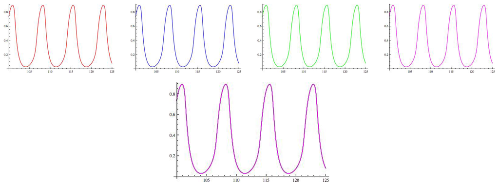
Figure 19.
Hop. Top: nodes 1–4; Bottom: all nodes. Parameter values: a = 1, b = 8, c = 1;ε = 0.67, g = 1.8; α = 0.5, γ = 0.8, β = 0.6; I = 0.8.
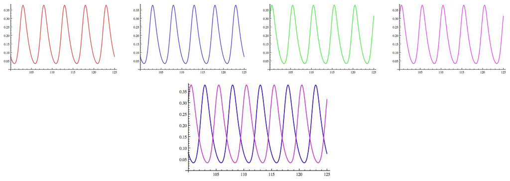
Figure 20.
Run. Top: nodes 1–4. Bottom: all nodes. Parameter values: a = 1, b = 8, c = 1; ε = 0.67, g = 1.8; α = −0.5,γ = 0.8, β = −0.6; I = 1.1.
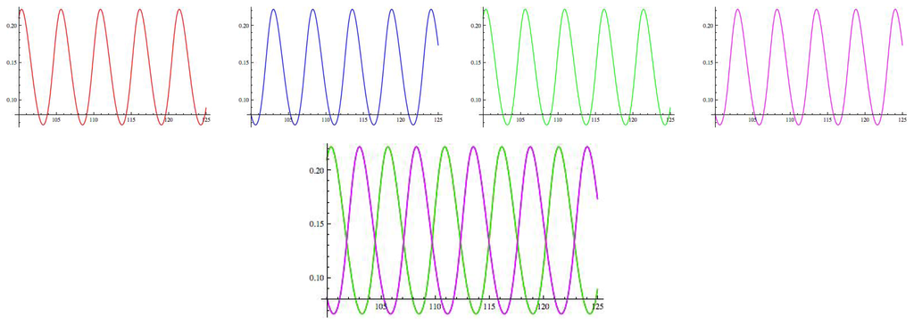
Figure 21.
Jump. Top: nodes 1–4. Bottom: all nodes. Parameter values: a = 1, b = 8, c = 1;ε = 0.67, g = 1.8; α = −0.5, γ= −0.8, β = 0.6; I = 1.1.
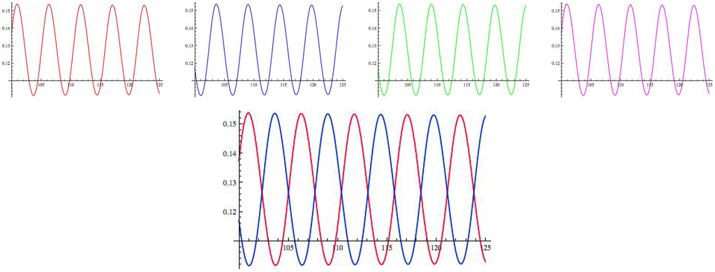
Figure 22.
Walk. Top: nodes 1–4. Bottom: all nodes. Parameter values: a = 1, b = 8, c = 1; ε = 0.67, g = 1.8; α = 0.5, γ = −0.8, β = −0.6; I = 1.1.
Acknowledgments
I am grateful to Marty Golubitsky for introducing me to rate equations and for many helpful conversations.
Conflicts of Interest
The author declares no conflict of interest.
References
- Gambaryan, P. How Mammals Run: Anatomical Adaptations; Wiley: New York, NY, USA, 1974. [Google Scholar]
- Muybridge, E. Animals in Motion; Chapman and Hall: London, UK, 1899; Reprinted Dover: New York, NY, USA, 1957.
- McGhee, R.B. Some finite state aspects of legged locomotion. Math. Biosci. 1968, 2, 67–84. [Google Scholar]
- Hildebrand, M. Vertebrate locomotion, an introduction: How does an animal's body move itself along? BioScience 1989, 39, 764–765. [Google Scholar]
- Kopell, N. Towards a Theory of Modelling Central Pattern Generators. In Neural Control of Rhythmic Movements in Vertebrates; Cohen, A.H., Rossignol, S., Grillner, S., Eds.; Wiley: New York, NY, USA, 1988. [Google Scholar]
- Kopell, N.; Ermentrout, G.B. Symmetry and phaselocking in chains of weakly coupled oscillators. Commun. Pure Appl. Math. 1986, 39, 623–660. [Google Scholar]
- Kopell, N.; Ermentrout, G.B. Coupled oscillators and the design of central pattern generators. Math. Biosci. 1988, 89, 14–23. [Google Scholar]
- Kopell, N.; Ermentrout, G.B. Phase transitions and other phenomena in chains of oscillators. SIAM J. Appl. Math. 1990, 50, 1014–1052. [Google Scholar]
- Collins, J.J.; Stewart, I. Symmetry-breaking bifurcation: A possible mechanism for 2:1 frequency-locking in animal locomotion. J. Math. Biol. 1992, 30, 827–838. [Google Scholar]
- Collins, J.J.; Stewart, I. Hexapodal gaits and coupled nonlinear oscillator models. Biol. Cybern. 1993, 68, 287–298. [Google Scholar]
- Collins, J.J.; Stewart, I. Coupled nonlinear oscillators and the symmetries of animal gaits. J. Nonlinear Sci. 1993, 3, 349–392. [Google Scholar]
- Collins, J.J.; Stewart, I. A group-theoretic approach to rings of coupled biological oscillators. Biol. Cybern. 1994, 71, 95–103. [Google Scholar]
- Hassard, B.D.; Kazarinoff, N.D.; Wan, Y.-H. Theory and Applications of Hopf Bifurcation; London Mathematical Society Lecture Note Series 41; Cambridge University Press: Cambridge, UK, 1981. [Google Scholar]
- Buono, P.-L. A Model of Central Pattern Generators for Quadruped Locomotion. Ph.D. Thesis, University of Houston, Houston, TX, USA, 1998. [Google Scholar]
- Buono, P.-L. Models of central pattern generators for quadruped locomotion: II. Secondary gaits. J. Math. Biol. 2001, 42, 327–346. [Google Scholar]
- Buono, P.-L.; Golubitsky, M. Models of central pattern generators for quadruped locomotion: I. Primary gaits. J. Math. Biol. 2001, 42, 291–326. [Google Scholar]
- Golubitsky, M.; Stewart, I. The Symmetry Perspective, Progress in Mathematics 200; Birkhäuser: Basel, Switzerland, 2002. [Google Scholar]
- Golubitsky, M.; Stewart, I.; Schaeffer, D.G. Singularities and Groups in Bifurcation Theory II; Applied Mathematics Series 69; Springer: New York, NY, USA, 1988. [Google Scholar]
- Golubitsky, M.; Stewart, I.; Buono, P.-L.; Collins, J.J. A modular network for legged locomotion. Physica D 1998, 115, 56–72. [Google Scholar]
- Golubitsky, M.; Stewart, I.; Collins, J.J.; Buono, P.-L. Symmetry in locomotor central pattern generators and animal gaits. Nature 1999, 401, 693–695. [Google Scholar]
- Pinto, C.A.; Golubitsky, M. Central pattern generators for bipedal locomotion. J. Math. Biol. 2006, 53, 474–489. [Google Scholar]
- Golubitsky, M.; Stewart, I. Nonlinear dynamics of networks: The groupoid formalism. Bull. Am. Math. Soc. 2006, 43, 305–364. [Google Scholar]
- Golubitsky, M.; Stewart, I.; Török, A. Patterns of synchrony in coupled cell networks with multiple arrows. SIAM J. Appl. Dyn. Syst. 2005, 4, 78–100. [Google Scholar]
- Stewart, I.; Golubitsky, M.; Pivato, M. Symmetry groupoids and patterns of synchrony in coupled cell networks. SIAM J. Appl. Dyn. Syst. 2003, 2, 609–646. [Google Scholar]
- Diekman, C.; Golubitsky, M.; Wang, Y. Derived patterns in binocular rivalry networks. J. Math. Neuro. 2013, 3. [Google Scholar] [CrossRef]
- Curtu, R. Mechanisms for oscillations in a biological competition model. Proc. Appl. Math. Mech. 2007, 7. [Google Scholar] [CrossRef]
- Curtu, R. Singular Hopf bifurcations and mixed-mode oscillations in a two-cell inhibitory neural network. Physica D 2010, 239, 504–514. [Google Scholar]
- Curtu, R.; Shpiro, A.; Rubin, N.; Rinzel, J. Mechanisms for frequency control in neuronal competition models. SIAM J. Appl. Dyn. Syst. 2008, 7, 609–649. [Google Scholar]
- Poston, T.; Stewart, I. Catastrophe Theory and Its Applications; Surveys and Reference Works in Mathematics 2; Pitman: London, UK, 1978. [Google Scholar]
- Zeeman, E.C. Catastrophe Theory: Selected Papers 1972–1977; Addison-Wesley: London, UK, 1977. [Google Scholar]
- Wilson, H.R. Computational evidence for a rivalry hierarchy in vision. Proc. Natl. Acad. Sci. USA 2003, 100, 14499–14503. [Google Scholar]
- Laing, C.R.; Chow, C.C. A spiking neuron model for binocular rivalry. J. Comput. Neurosci. 2002, 12, 39–53. [Google Scholar]
- Shpiro, A.; Curtu, R.; Rinzel, J.; Rubin, N. Dynamical characteristics common to neuronal competition models. J. Neurophysiol. 2007, 97, 462–473. [Google Scholar]
- Wilson, H.R. Requirements for Conscious Visual Processing. In Cortical Mechanisms of Vision; Jenkin, M., Harris, L., Eds.; Cambridge University Press: Cambridge, UK, 2009; pp. 399–417. [Google Scholar]
- Diekman, C.; Golubitsky, M. Algorithm for Constructing and Analyzing Wilson Networks for Binocular Rivalry Experiments; MBI: Columbus, OH, USA, 2014; in press. [Google Scholar]
- Diekman, C.; Golubitsky, M.; McMillen, T.; Wang, Y. Reduction and dynamics of a generalized rivalry network with two learned patterns. SIAM J. Appl. Dyn. Syst. 2012, 11, 1270–1309. [Google Scholar]
- Diekman, C.; Golubitsky, M.; Stewart, I. Modelling visual illusions using generalised Wilson networks; Mathematics Institute, University of Warwick: Coventry, UK, Unpublished work; 2013. [Google Scholar]
- Golubitsky, M.; Stewart, I. Hopf bifurcation in the presence of symmetry. Arch. Ration. Mech. Anal. 1985, 87, 107–165. [Google Scholar]
- Cicogna, G. Symmetry breakdown from bifurcations. Lett. Nuovo Cimento 1981, 31, 600–602. [Google Scholar]
- Vanderbauwhede, A. Local Bifurcation and Symmetry. Habilitation Thesis, Rijksuniversiteit Gent, Gent, Belgium, 1980. [Google Scholar]
- Vanderbauwhede, A. Local Bifurcation and Symmetry Research Notes in Mathematics Series 75; Pitman: London, UK, 1982. [Google Scholar]
- Adams, J.F. Lectures on Lie Groups; University of Chicago Press: Chigago, IL, USA, 1969. [Google Scholar]
- Rotman, J.J. An Introduction to the Theory of Groups; Allyn and Bacon: Boston, TX, USA, 1984. [Google Scholar]
- Hall, M., Jr. The Theory of Groups; Macmillan: New York, NY, USA, 1959. [Google Scholar]
- Loney, S.L. The Elements of Coordinate Geometry; Macmillan: London, UK, 1960. [Google Scholar]
- Guckenheimer, J.; Holmes, P. Nonlinear Oscillations, Dynamical Systems, and Bifurcations of Vector Fields; Applied Mathematical Sciences; Vol. 42, Springer: New York, NY, USA, 1990. [Google Scholar]
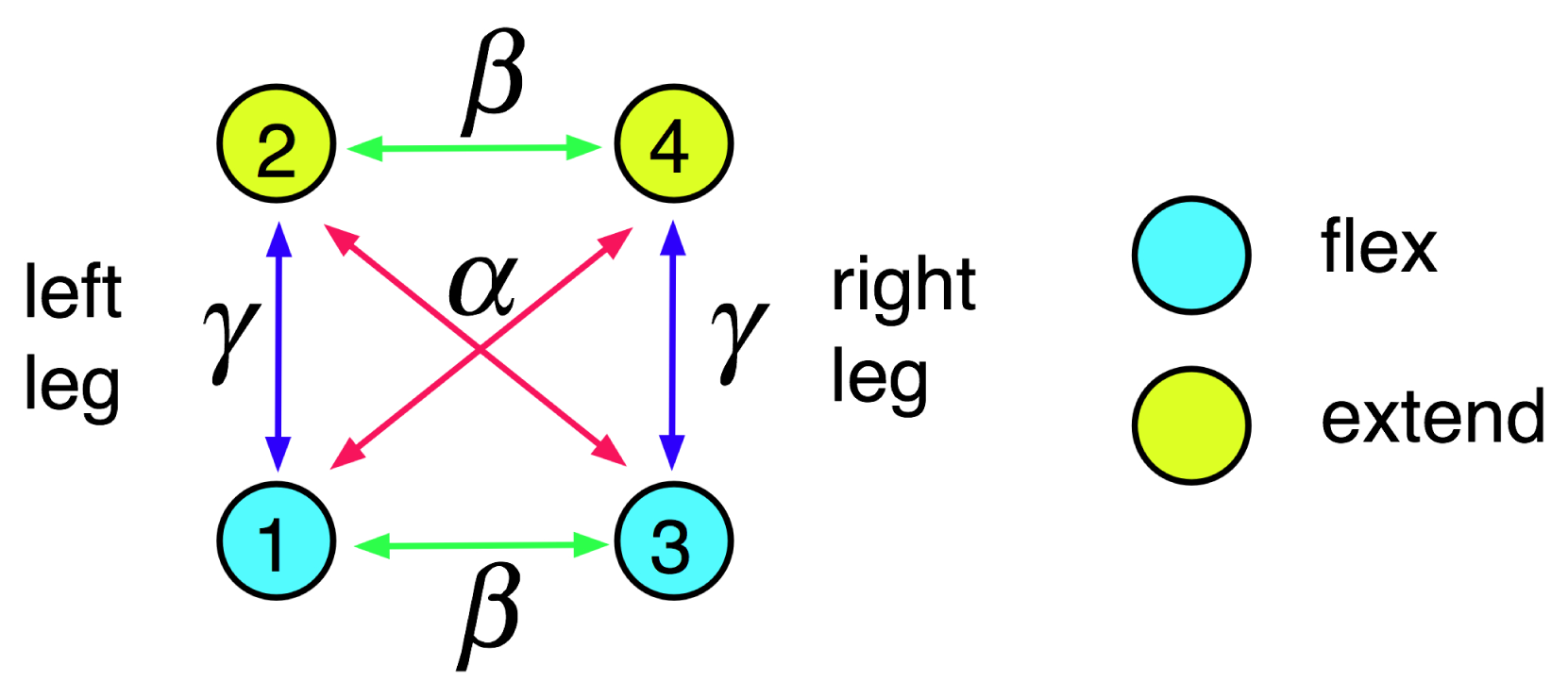

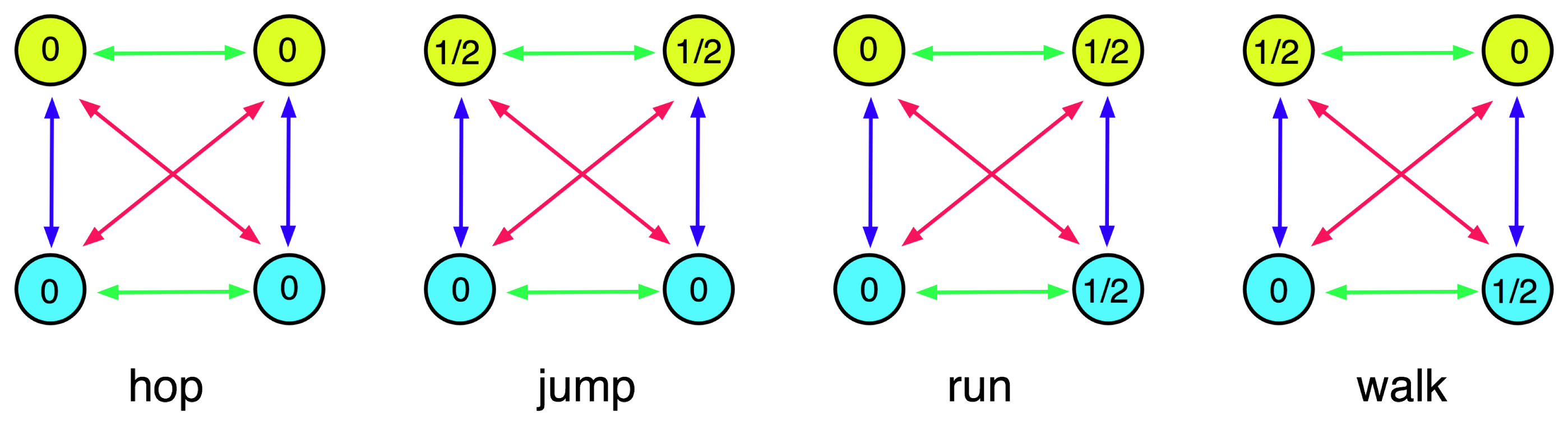

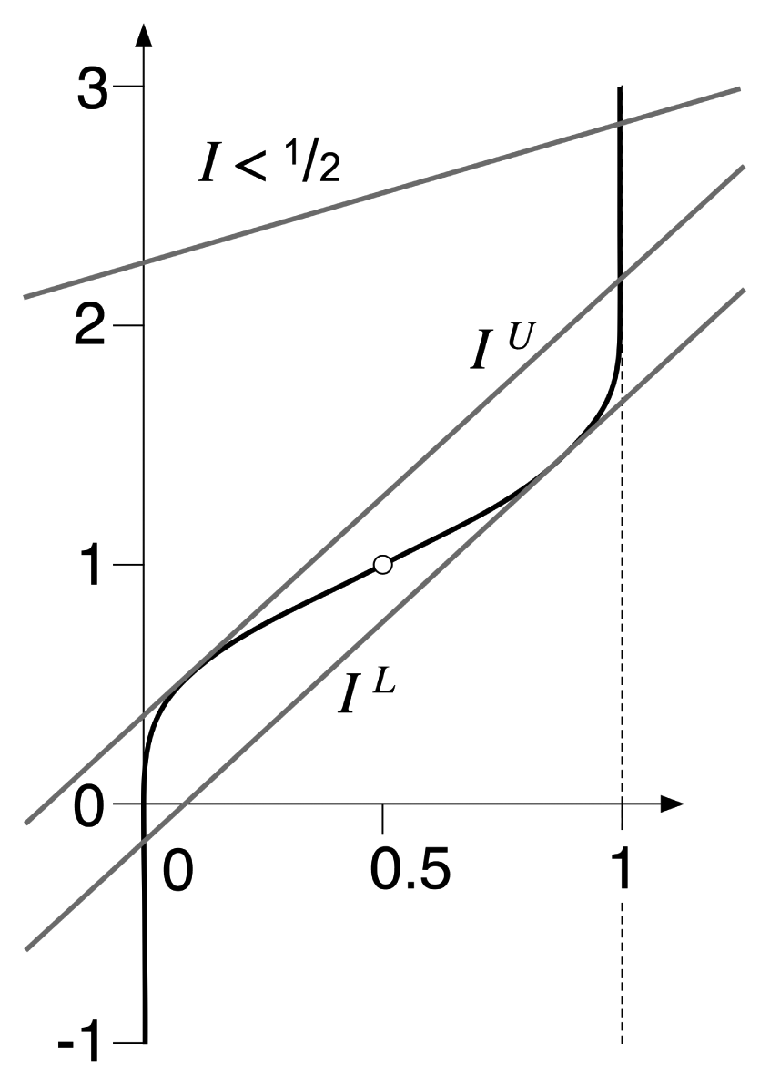
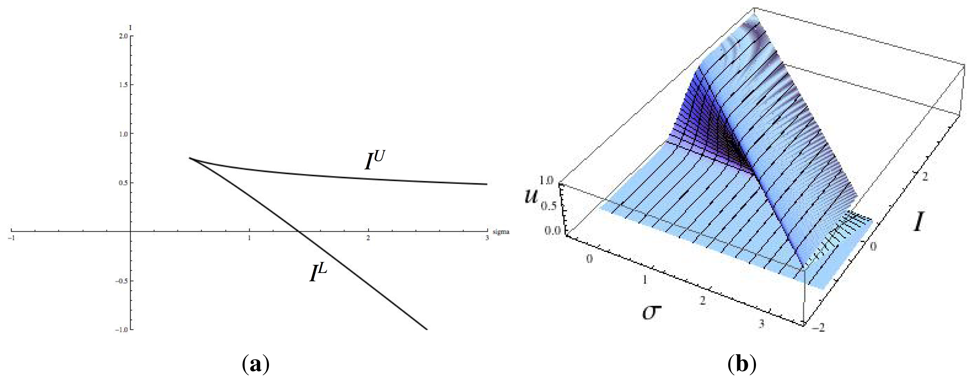
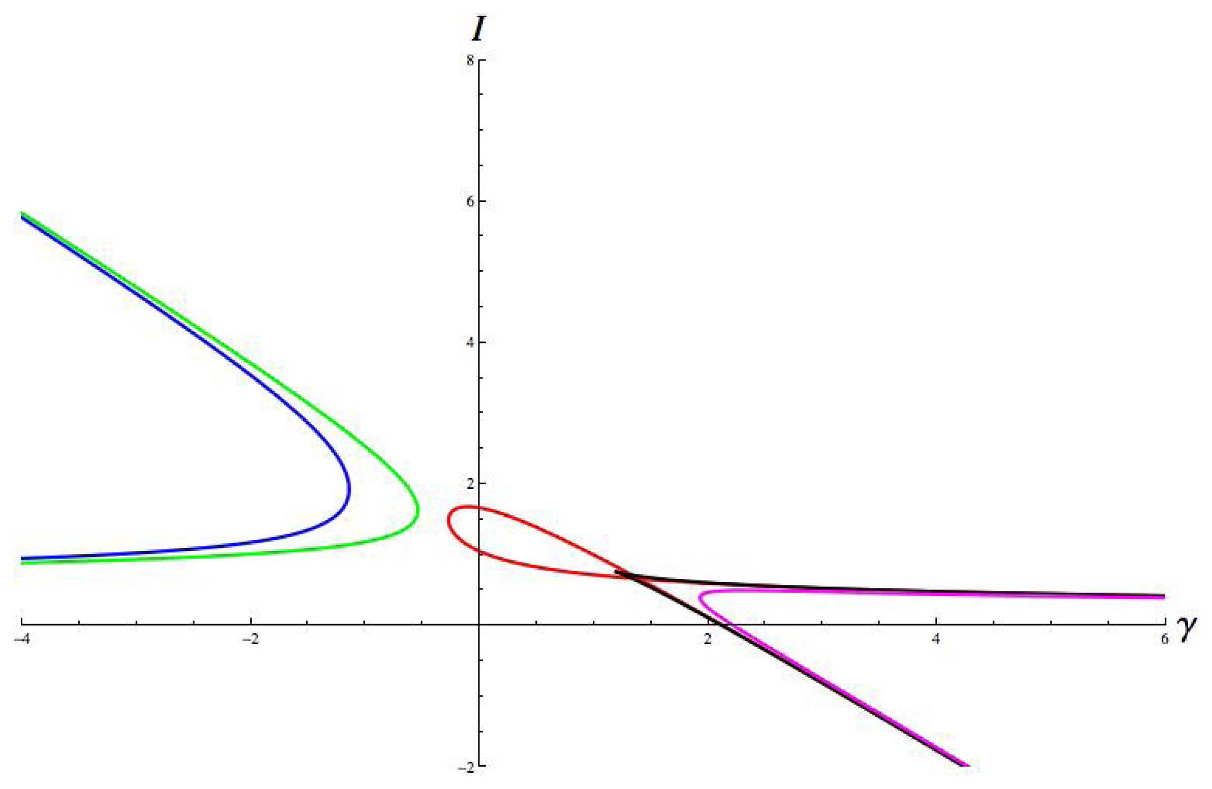
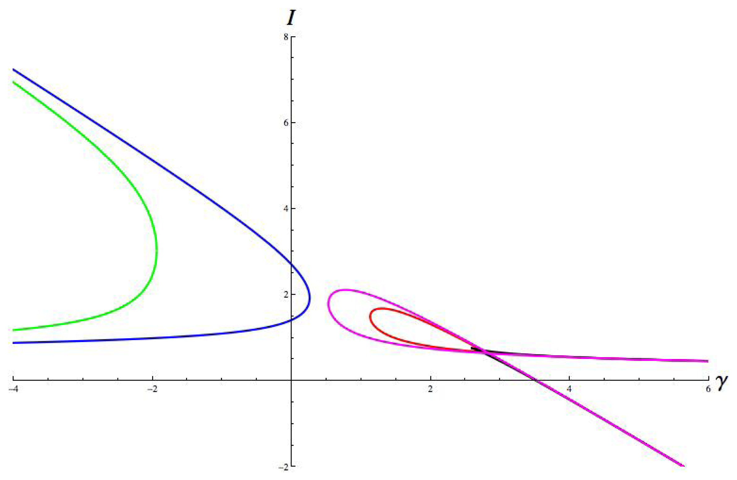
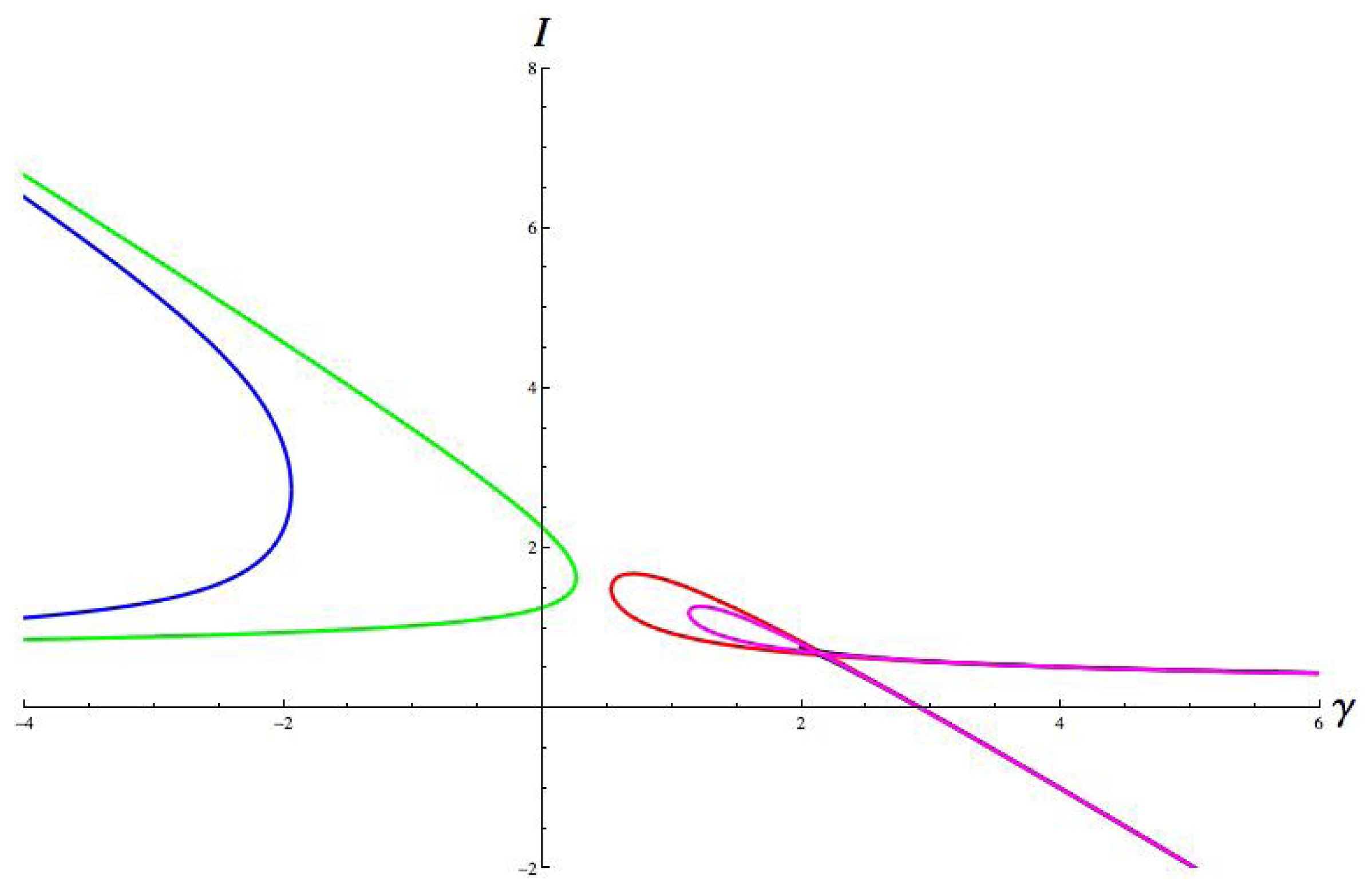

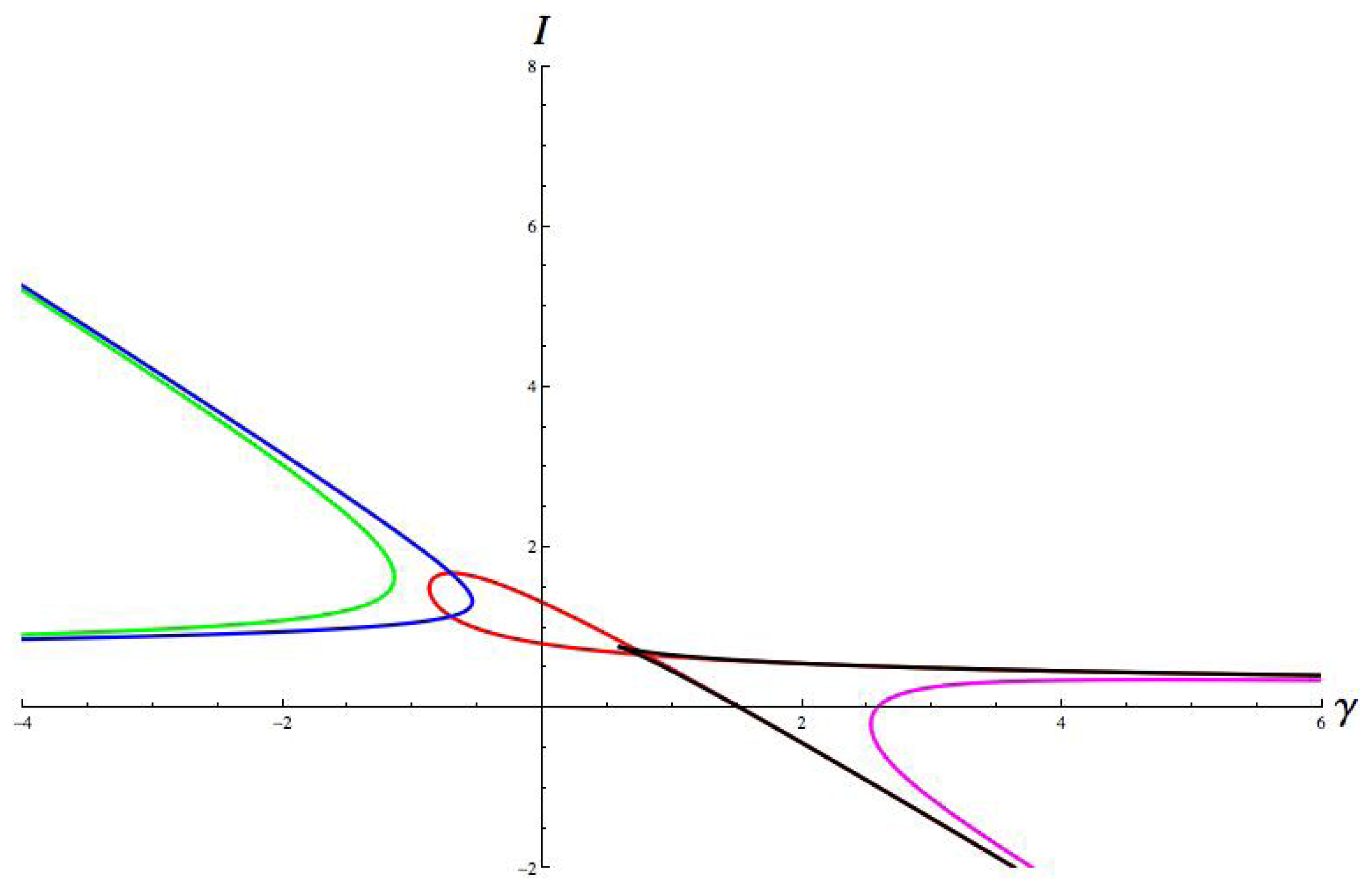
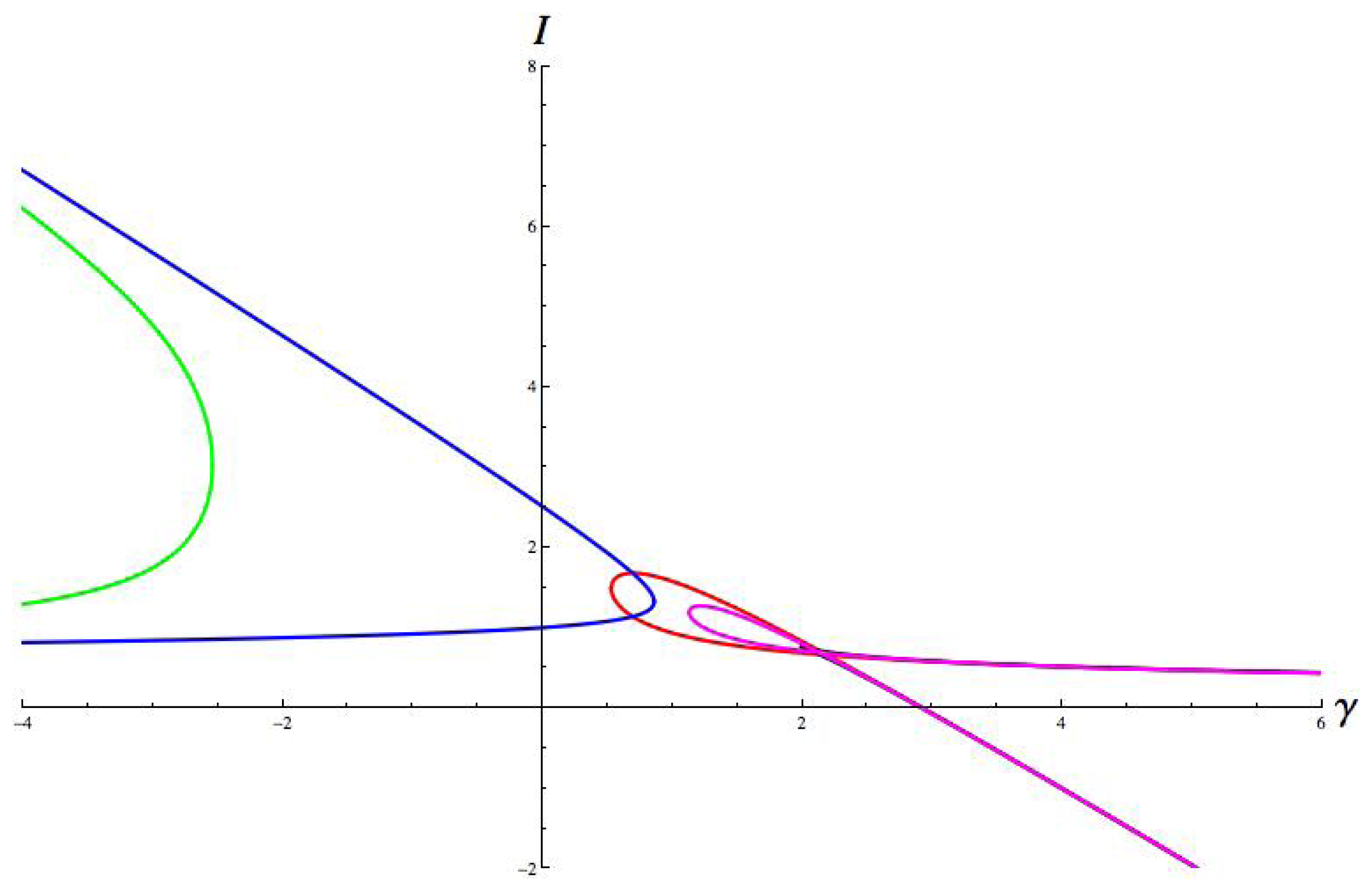
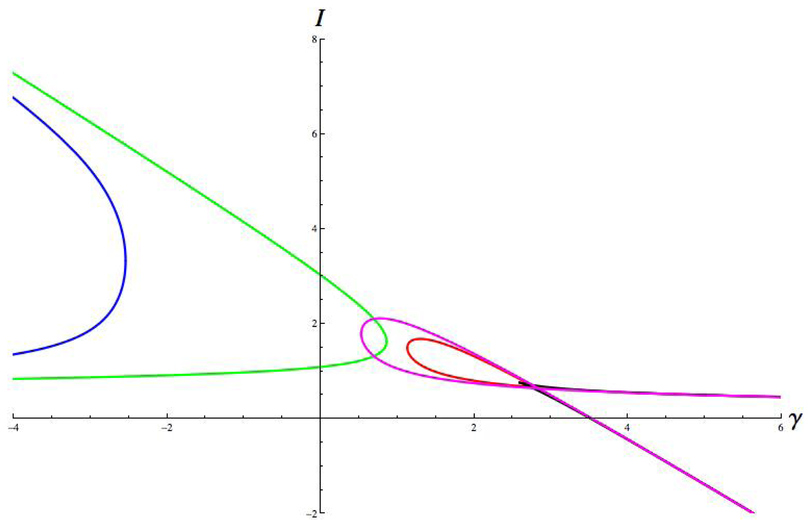
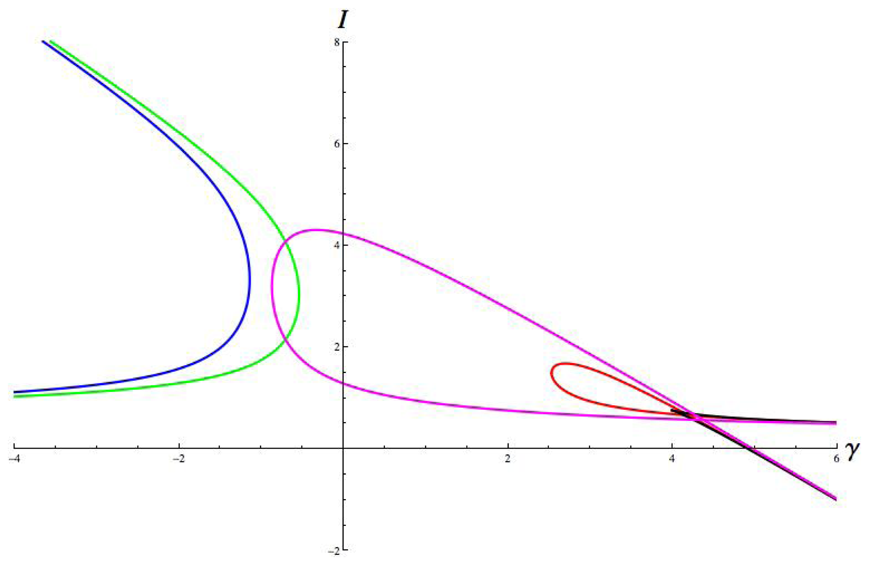
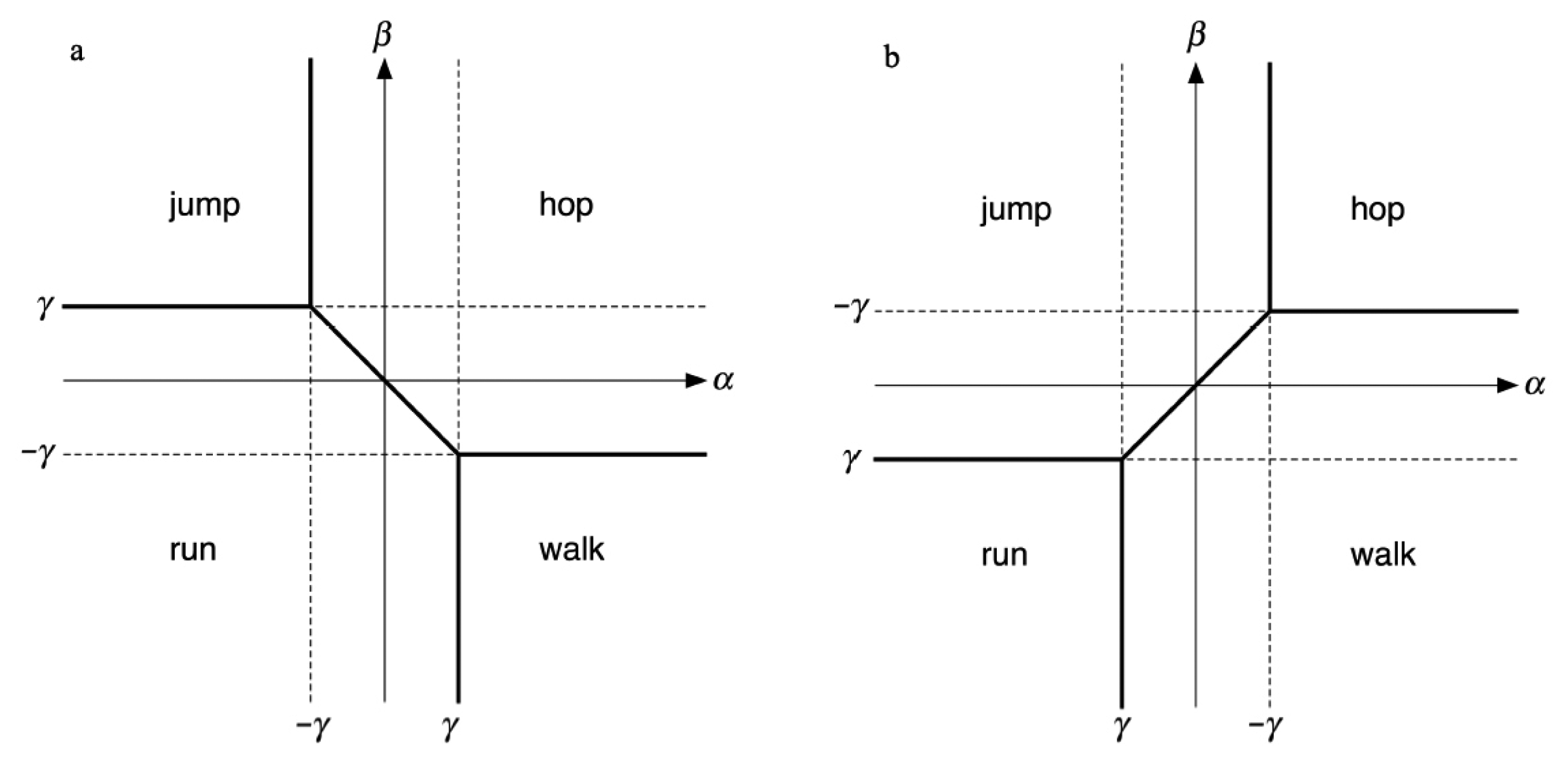
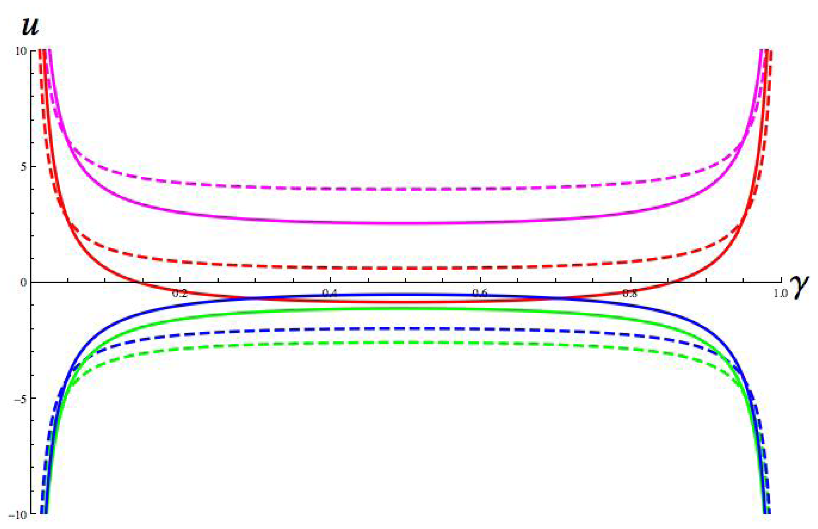
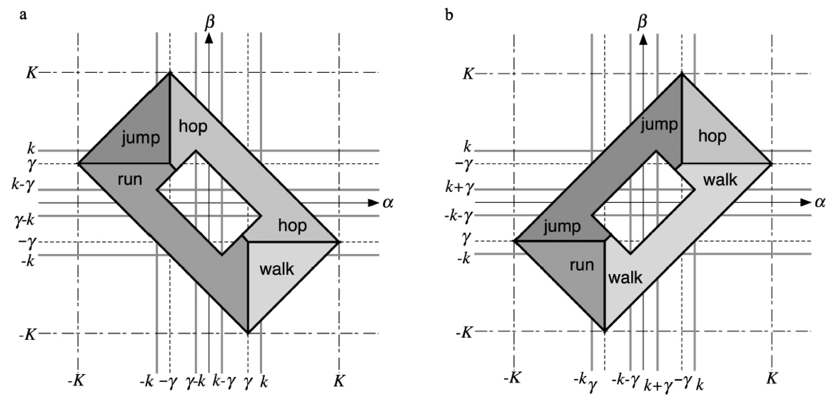

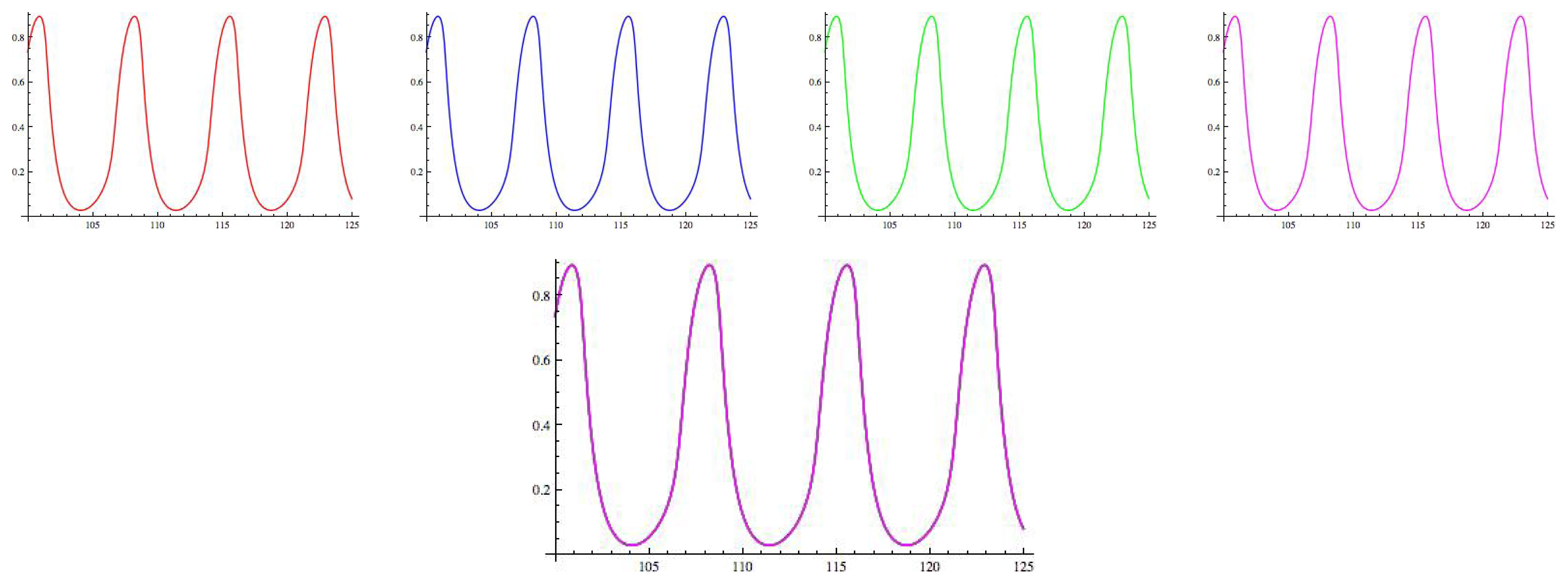
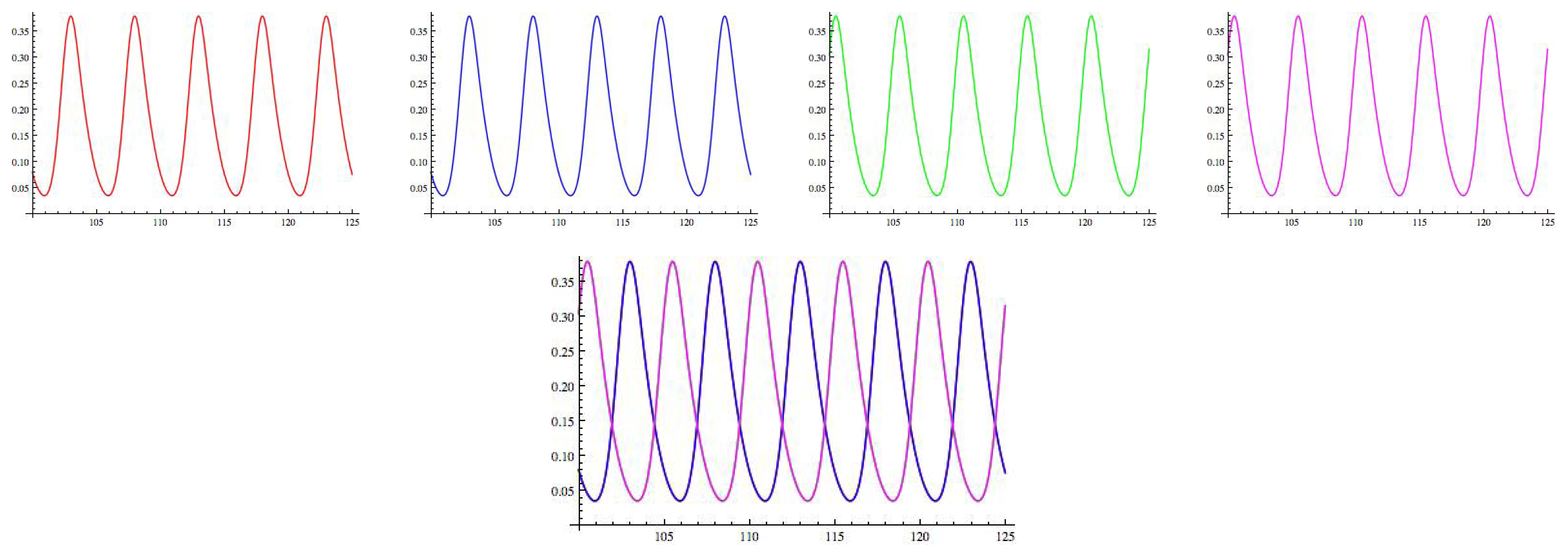
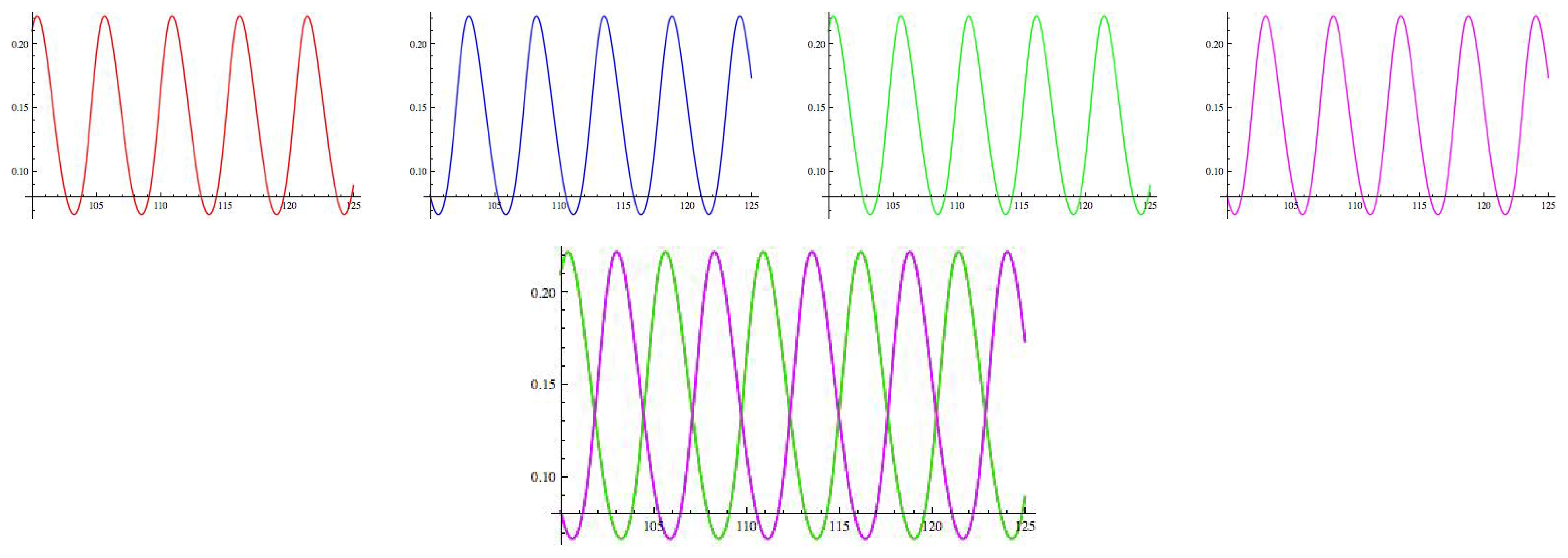
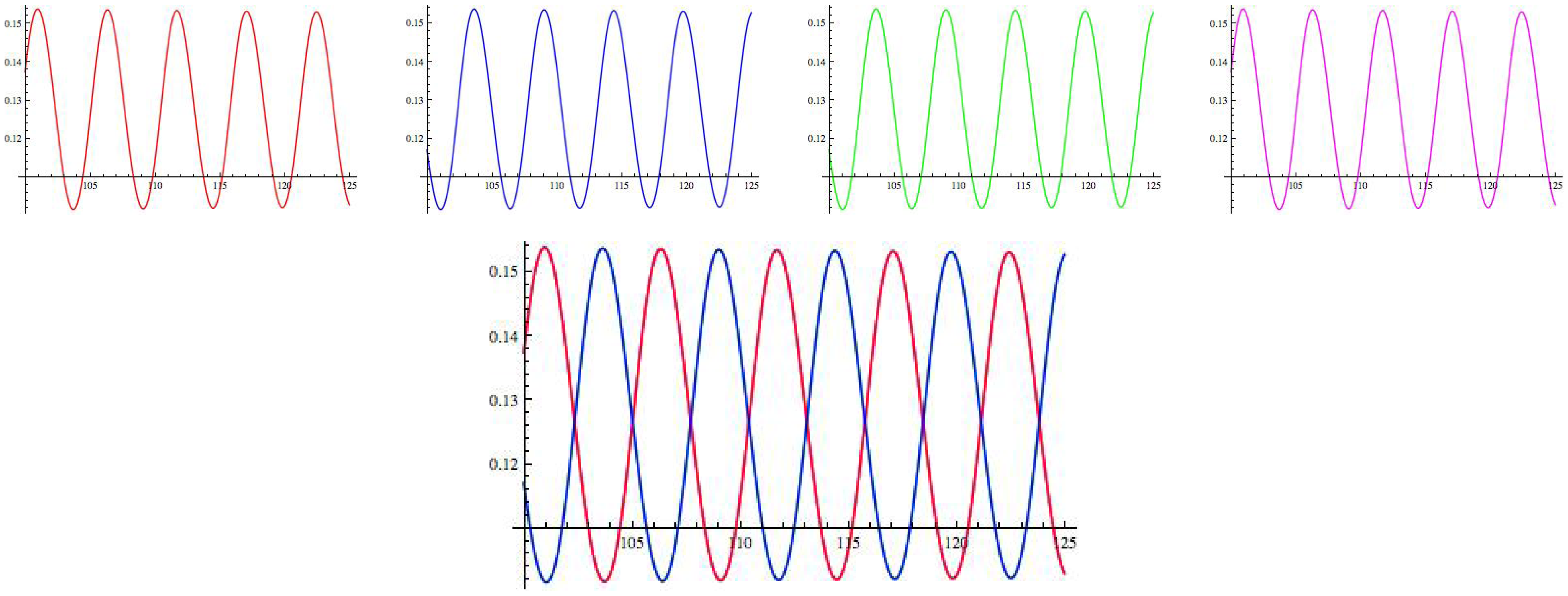
© 2014 by the authors; licensee MDPI, Basel, Switzerland. This article is an open access article distributed under the terms and conditions of the Creative Commons Attribution license ( http://creativecommons.org/licenses/by/3.0/).