On Symmetry of Independence Polynomials

Abstract

An independent set in a graph is a set of pairwise non-adjacent vertices, and $\alpha \left(G\right)$ is the size of a maximum independent set in the graph G. A matching is a set of non-incident edges, while $\mu \left(G\right)$ is the cardinality of a maximum matching. If $s_k$ is the number of independent sets of size k in G, then $I(G;x)=s_0+s_{1}x+s_2{x}^2+\dots +s_{\alpha }{x}^{\alpha }$, $\alpha =\alpha \left(G\right)$, is called the independence polynomial of G (Gutman and Harary, 1986). If $s_j=s_{\alpha -j}$ for all $0\le j\le ⌊\alpha /2⌋$, then $I(G;x)$ is called symmetric (or palindromic). It is known that the graph $G\circ 2K_1$, obtained by joining each vertex of G to two new vertices, has a symmetric independence polynomial (Stevanović, 1998). In this paper we develop a new algebraic technique in order to take care of symmetric independence polynomials. On the one hand, it provides us with alternative proofs for some previously known results. On the other hand, this technique allows to show that for every graph G and for each non-negative integer $k\le \mu \left(G\right)$, one can build a graph H, such that: G is a subgraph of H, $I\left(H;x\right)$ is symmetric, and $I\left(G\circ 2K_1;x\right)={\left(1+x\right)}^k·I\left(H;x\right)$.

1. Introduction

Throughout this paper $G=(V,E)$ is a simple (i.e., a finite, undirected, loopless and without multiple edges) graph with vertex set $V=V\left(G\right)$ and edge set $E=E\left(G\right).$ If $X\subset V$, then $G\left[X\right]$ is the subgraph of G spanned by X. By $G-W$ we mean the subgraph $G[V-W]$, if $W\subset V\left(G\right)$. We also denote by $G-F$ the partial subgraph of G obtained by deleting the edges of F, for $F\subset E\left(G\right)$, and we write shortly $G-e$, whenever F $=\{e\}$.

The neighborhood of a vertex $v\in V$ is the set $N_G\left(v\right)=\{w:w\in V$ and $vw\in E\}$, while $N_G\left[v\right]=N_G\left(v\right)\cup \{v\}$; if there is no ambiguity on G, we write $N\left(v\right)$ and $N\left[v\right]$.

$K_n,P_n,C_n$ denote, respectively, the complete graph on $n\ge 1$ vertices, the chordless path on $n\ge 1$ vertices, and the chordless cycle on $n\ge 3$ vertices.

The disjoint union of the graphs $G_1,G_2$ is the graph $G=G_1\cup G_2$ having as vertex set the disjoint union of $V\left(G_1\right),V\left(G_2\right)$, and as edge set the disjoint union of $E\left(G_1\right),E\left(G_2\right)$. In particular, $nG$ denotes the disjoint union of $n>1$ copies of the graph G.

If $G_1,G_2$ are disjoint graphs, $A_1\subseteq V\left(G_1\right),A_2\subseteq V\left(G_2\right)$, then the Zykov sum of $G_1,G_2$ with respect to $A_1,A_2$, is the graph $\left(G_1,A_1\right)+(G_2,A_2)$ with $V\left(G_1\right)\cup V\left(G_2\right)$ as vertex set and

$$E\left(G_1\right)\cup E\left(G_2\right)\cup \{v_1{v}_2:v_1\in A_1,v_2\in A_2\}$$

as edge set [1]. If $A_1=V\left(G_1\right)$ and $A_2=V\left(G_2\right)$, we simply write $G_1+G_2$.

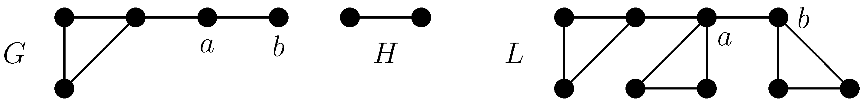
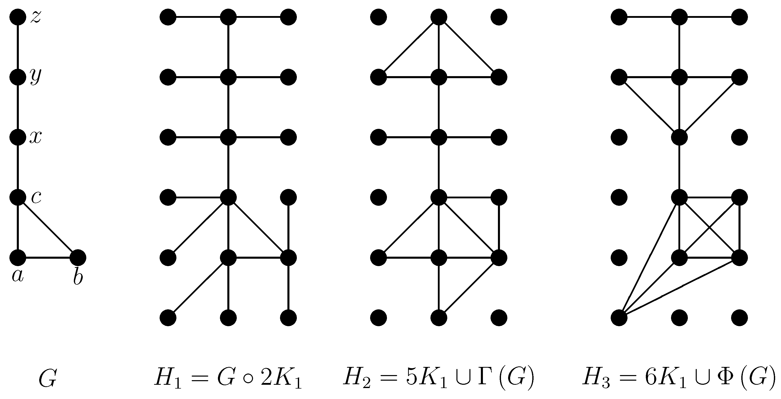
The corona of the graphs G and H with respect to $A\subseteq V\left(G\right)$ is the graph $\left(G,A\right)\circ H$ obtained from G and $\left|A\right|$ copies of H, such that every vertex belonging to A is joined to all vertices of a copy of H [2]. If $A=$$V\left(G\right)$ we use $G\circ H$ instead of $\left(G,V\left(G\right)\right)\circ H$ (see Figure 1 for an example).

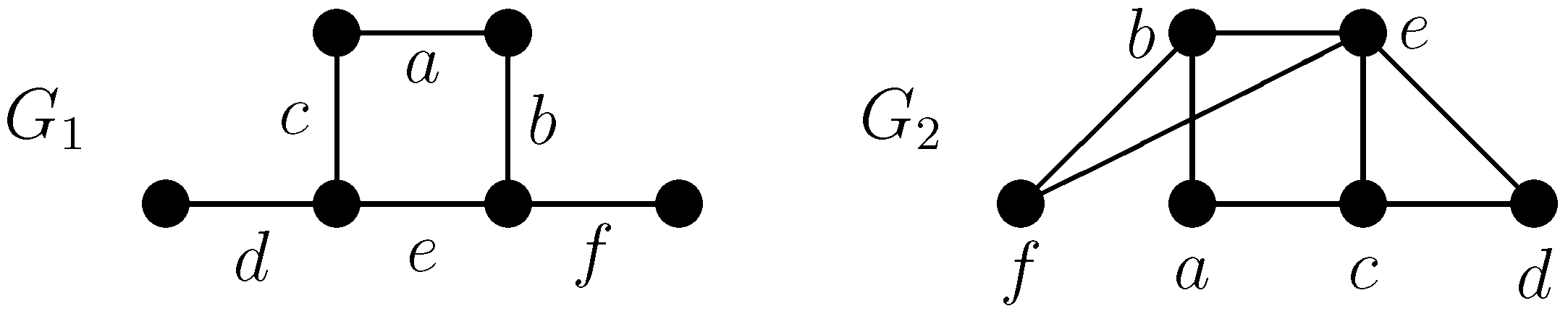
Let $G,H$ be two graphs and C be a cycle on q vertices of G. By $(G,C)△H$ we mean the graph obtained from G and q copies of H, such that each two consecutive vertices on C are joined to all vertices of a copy of H (see Figure 2 for an example).

An independent (or a stable) set in G is a set of pairwise non-adjacent vertices. By $Ind\left(G\right)$ we mean the family of all independent sets of G. An independent set of maximum size will be referred to as a maximum independent set of G, and the independence number of G, denoted by $\alpha \left(G\right)$, is the cardinality of a maximum independent set in G.

Let $s_k$ be the number of independent sets of size k in a graph G. The polynomial

$$I(G;x)=s_0+s_{1}x+s_2{x}^2+\dots +s_{\alpha }{x}^{\alpha },\alpha =\alpha \left(G\right)$$

is called the independence polynomial of G [3,4], the independent set polynomial of G [5]. In [6], the dependence polynomial $D(G;x)$ of a graph G is defined as $D(G;x)=I(\overline{G};-x)$.

A matching is a set of non-incident edges of a graph G, while $\mu \left(G\right)$ is the cardinality of a maximum matching. Let $m_k$ be the number of matchings of size k in G.

The polynomial

$$M(G;x)=m_0+m_{1}x+m_2{x}^2+\dots +m_{\mu }{x}^{\mu },\mu =\mu \left(G\right)$$

is called the matching polynomial of G [7].

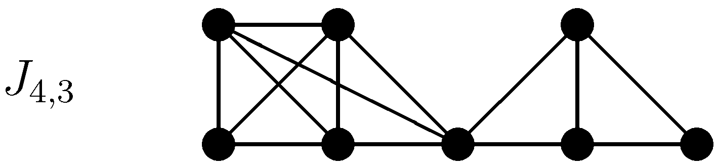
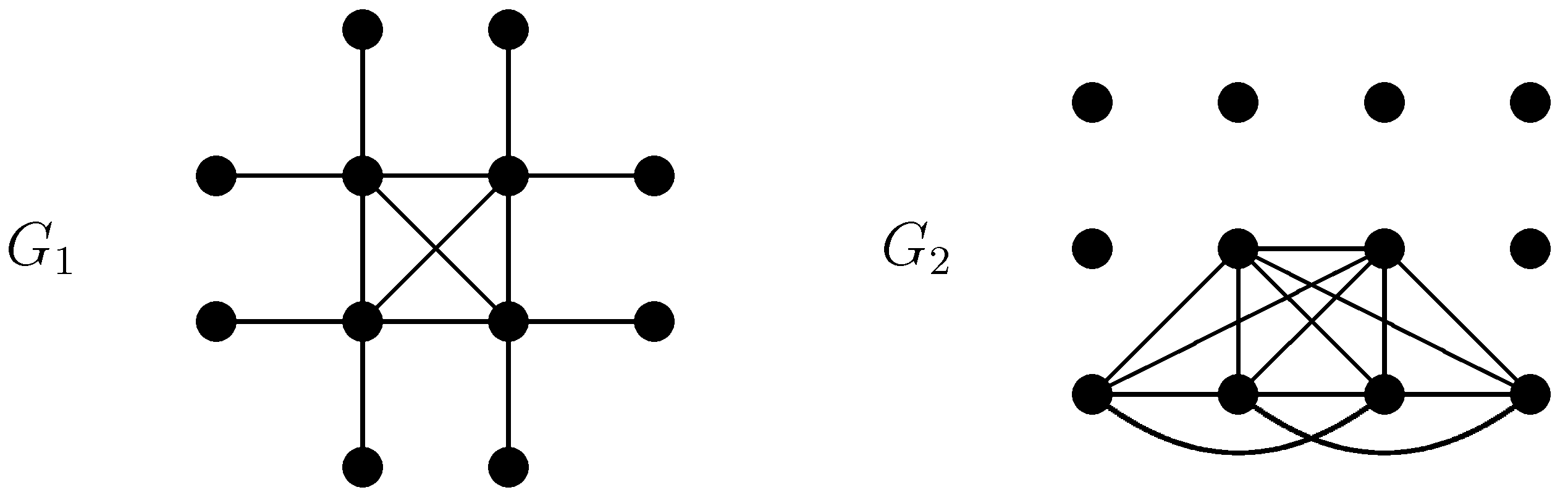
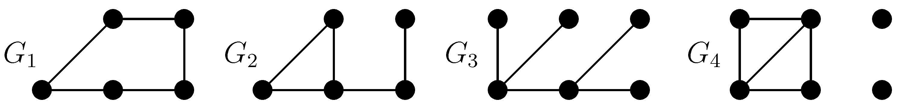
The independence polynomial has been defined as a generalization of the matching polynomial, because the matching polynomial of a graph G and the independence polynomial of its line graph are identical. Recall that given a graph G, its line graph $L\left(G\right)$ is the graph whose vertex set is the edge set of G, and two vertices are adjacent if they share an end in G. For instance, the graphs $G_1$ and $G_2$ depicted in Figure 3 satisfy $G_2=L\left(G_1\right)$ and, hence, $I(G_2;x)=1+6x+7x^2+x^3=M(G_1;x)$.

In [3] a number of general properties of the independence polynomial of a graph are presented. As examples, we mention that:

$$I(G_1\cup G_2;x)=I(G_1;x)·I(G_2;x),I(G_1+G_2;x)=I(G_1;x)+I(G_2;x)-1.$$

The following equalities are very useful in calculating of the independence polynomial for various families of graphs.

Theorem 1.1.

Let $G=(V,E)$ be a graph of order n. Then the following identities are true:

(i) $I(G;x)=I(G-v;x)+x·I(G-N[v];x)$ holds for each $v\in V$ [3].

(ii) $I\left(G\circ H;x\right)={\left(I\left(H;x\right)\right)}^n·I\left(G;\frac{x}{I\left(H;x\right)}\right)$ for every graph H [8].

A finite sequence of real numbers $(a_0,a_1,a_2,\dots ,a_n)$ is said to be:

• unimodal if there is some $k\in \{0,1,\dots ,n\}$, such that $a_0\le \dots \le a_{k-1}\le a_k\ge a_{k+1}\ge \dots \ge a_n$;
• log-concave if $a_i^2\ge a_{i-1}·a_{i+1},i\in \{1,2,\dots ,n-1\}$;
• symmetric (or palindromic) if $a_i=a_{n-i},i=0,1,\dots ,⌊n/2⌋$.

It is known that every log-concave sequence of positive numbers is also unimodal.

A polynomial is called unimodal (log-concave, symmetric) if the sequence of its coefficients is unimodal (log-concave, symmetric, respectively).

For instance, the independence polynomial:

• $I(K_{42}+3K_7;x)=1+63x+147x^2+343x^3$ is log-concave;
• $I(K_{43}+3K_7;x)=1+64x+147x^2+343x^3$ is unimodal, but it is not log-concave, because $147·147-64·343=-343<0$;
• $I(K_{127}+3K_7;x)=1+148x+\mathbf{147}{x}^2+343x^3$ is non-unimodal;
• $I(K_{18}+3K_3+4K_1;x)=1+31x+33x^2+31x^3+x^4$ is symmetric and log-concave;
• $I(K_{52}+3K_4+4K_1;x)=1+68x+54x^2+68x^3+x^4$ is symmetric and non-unimodal.

It is easy to see that if $\alpha \left(G\right)\le 3$ and $I(G;x)$ is symmetric, then it is also log-concave.

For other examples, see [9,10,11,12,13,14]. Alavi et al. proved that for every permutation $\pi$ of $\{1,2,\dots ,\alpha \}$ there is a graph G with $\alpha \left(G\right)=\alpha$ such that $s_{\pi \left(1\right)}<s_{\pi \left(2\right)}<\dots <s_{\pi \left(\alpha \right)}$ [9].

The following conjecture is still open.

Conjecture 1.2.

The independence polynomial of every tree is unimodal [9].

Hence to prove the unimodality of independence polynomials is sometimes a difficult task. Moreover, even if the independence polynomials of all the connected components of a graph G are unimodal, then $I(G;x)$ is not for sure unimodal [15]. The following result shows that symmetry gives a hand to unimodality.

Theorem 1.3.

If P and Q are both unimodal and symmetric, then $P·Q$ is unimodal and symmetric [16].

A clique cover of a graph G is a spanning graph of G, each connected component of which is a clique. A cycle cover of a graph G is a spanning graph of G, each connected component of which is a vertex, an edge, or a proper cycle. In this paper we give an alternative proof for the fact that the polynomials $I(G\circ 2K_1;x)$, $I(\Phi (G);x)$, and $I(\Gamma (G);x)$ are symmetric for every clique cover $\Phi$, and every cycle cover $\Gamma$ of a graph G, where $\Phi \left(G\right)$ and $\Gamma \left(G\right)$ are graphs built by Stevanović’s rules [17]. Our main finding claims that the polynomial $I(G\circ 2K_1;x)$ is divisible both by $I(\Phi (G);x)$ and $I(\Gamma (G);x)$.

The paper is organized as follows. Section 2 looks at previous results on symmetric independence polynomials, Section 3 presents our results connecting symmetric independence polynomials derived by Stevanović’s rules [17], while Section 4 is devoted to conclusions, future directions of research, and some open problems.

2. Related Work

The symmetry of the matching polynomial and the characteristic polynomial of a graph were examined in [18], while for the independence polynomial we quote [17,19,20]. Recall from [18] that G is called an equible graph if $G=H\circ K_1$ for some graph H. Both matching polynomials and characteristic polynomials of equible graphs are symmetric [18]. Nevertheless, there are non-equible graphs whose matching polynomials and characteristic polynomials are symmetric.

It is worth mentioning that one can produce graphs with symmetric independence polynomials in different ways. For instance, the independence polynomial of the disjoint union of two graphs having symmetric independence polynomial is symmetric as well. Another basic graph operation preserving symmetry of the independence polynomial is the Zykov sum of two graphs with the same independence number. We summarize other constructions respecting symmetry of the independence polynomial in what follows.

2.1. Gutman’s Construction [21]

For integers $p>1$, $q>1$, let $J_{p,q}$ be the graph built in the following manner [21]. Start with three complete graphs $K_1$, $K_p$ and $K_q$ whose vertex sets are disjoint. Connect the vertex of $K_1$ with $p-1$ vertices of $K_p$ and with $q-1$ vertices of $K_q$ (see Figure 4 as an example).

The graph thus obtained has a unique maximum independent set of size three, and its independence polynomial is equal to

$$I\left(J_{p,q};x\right)=1+(p+q+1)x+(pq+2)x^2+x^3.$$

Hence the independence polynomial of $G=J_{p,q}+K_{pq-p-q+1}$ is

$$I\left(G;x\right)=I\left(J_{p,q};x\right)+I\left(K_{pq-p-q+1};x\right)-1=1+\left(2+pq\right)x+\left(2+pq\right)x^2+x^3,$$

which is clearly symmetric and log-concave.

2.2. Bahls and Salazar’s Construction [20]

The $K_t$-path of length $k\ge 1$ is the graph $P(t,k)=(V,E)$ with $V=\{v_1,v_2,\dots ,v_{t+k-1}\}$ and $E=\left\{v_i{v}_{i+j}:1\le i\le t+k-2,1\le j\le min\{t-1,t+k-i-1\}\right\}$. Such a graph consists of k copies of $K_t$, each glued to the previous one by identifying certain prescribed subgraphs isomorphic to $K_{t-1}$. Let $d\ge 0$ be an integer. The d-augmented $K_t$ path $P(t,k,d)$ is defined by introducing new vertices ${\{u_{{}_i,1},u_{{}_i,2},\dots ,u_{i,d}\}}_{i=0}^{t+k-2}$ and edges ${\left\{v_i{u}_{i,j},v_{i+1}{u}_{i,j}:j=1,\dots ,d\right\}}_{i=1}^{t+k-2}\cup \left\{v_1,u_{0,j}:j=1,\dots ,d\right\}$. Let $G=(V,E)$ and $U\subseteq V$ be a subset of its vertices. Let $v\notin V$ and define the cone of G on U with vertex v, denoted $G^{*}(U,v)=\left(G,U\right)+K_1$, where $K_1=\left(\left\{v\right\},\varnothing \right)$. Given G and U and a graph H, we write $H+\left(G,U\right)$ instead of $\left(H,V\left(H\right)\right)+\left(G,U\right)$.

Theorem 2.1.

Let $t\ge 2,k\ge 1$, and $d\ge 0$ be integers, and let $G=(V,E)$ be a graph with $U\subseteq V$ a distinguished subset of vertices. Suppose that each of the graphs G, $G-U$, and $\left(G,U\right)+K_1$ has a symmetric and unimodal independence polynomial, and $deg\left(I(G;x)\right)=deg\left(I(\left(G,U\right)+K_1;x)\right)=deg\left(I(G-U;x)\right)+2$. Then the independence polynomial of the graph $P(t,k,d)+(G,U)$ is symmetric and unimodal [20].

2.3. Stevanović’s Constructions [17]

Taking into account that $s_0=1$ and $s_1=\left|V\left(G\right)\right|=n$, it follows that if $I(G;x)$ is symmetric, then $s_0=s_{\alpha }$ and $s_1=s_{\alpha -1}$, i.e., G has only one maximum independent set, say S, and $n-\alpha \left(G\right)$ independent sets, of size $\alpha \left(G\right)-1$, that are not subsets of S.

Theorem 2.2.

If there is an independent set S in G such that $\left|N\left(A\right)\cap S\right|=2\left|A\right|$ holds for every independent set $A\subseteq V\left(G\right)-S$, then $I(G;x)$ is symmetric [17].

The following result is a consequence of Theorem 2.2.

Corollary 2.3.

(i) If $\alpha \left(G\right)=\alpha ,s_{\alpha }=1,s_{\alpha -1}=\left|V\left(G\right)\right|$, and for the unique stability system S of G it is true that $\left|N\left(v\right)\cap S\right|=2$ for each $v\in V\left(G\right)-S$, then $I(G;x)$ is symmetric [17]; (ii) If G is a claw-free graph with $\alpha \left(G\right)=\alpha ,s_{\alpha }=1,s_{\alpha -1}=\left|V\left(G\right)\right|$, then $I(G;x)$ is symmetric.

Corollary 2.3 gives three different ways to construct graphs having symmetric independence polynomials [17].

• Rule 1. For a given graph G, define a new graph H as: $H=G\circ 2K_1$.

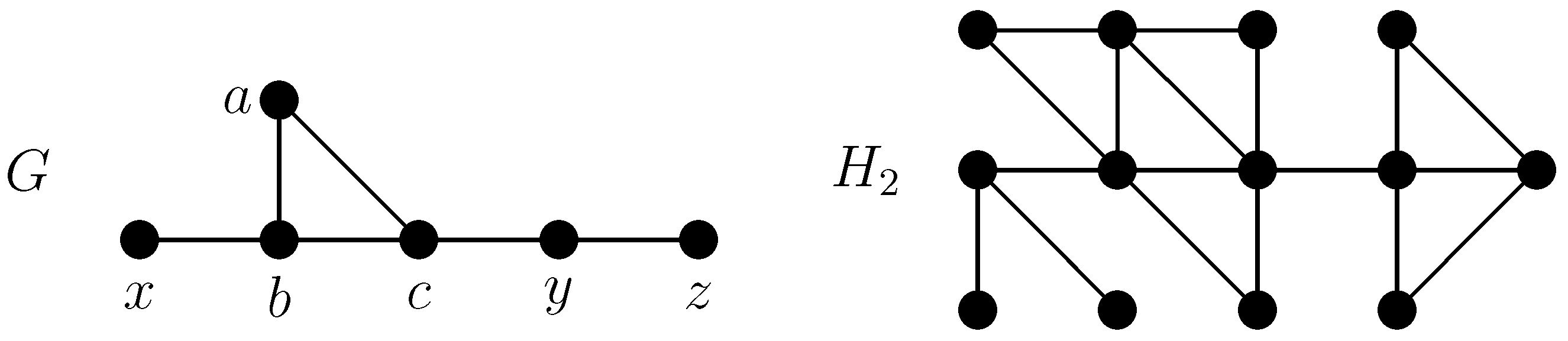
For an example, see the graphs in Figure 5: $I(G;x)=1+6x+9x^2+3x^3$, while

$$I(H_1;x)={\left(1+x\right)}^6\left(1+12x+48x^2+77x^3+48x^4+12x^5+x^6\right)=$$

$$=1+18x+135x^2+565x^3+1485x^4+2601x^5+3126x^6+2601x^7+1485x^8+565x^9+135x^{10}+18x^{11}+x^{12}.$$

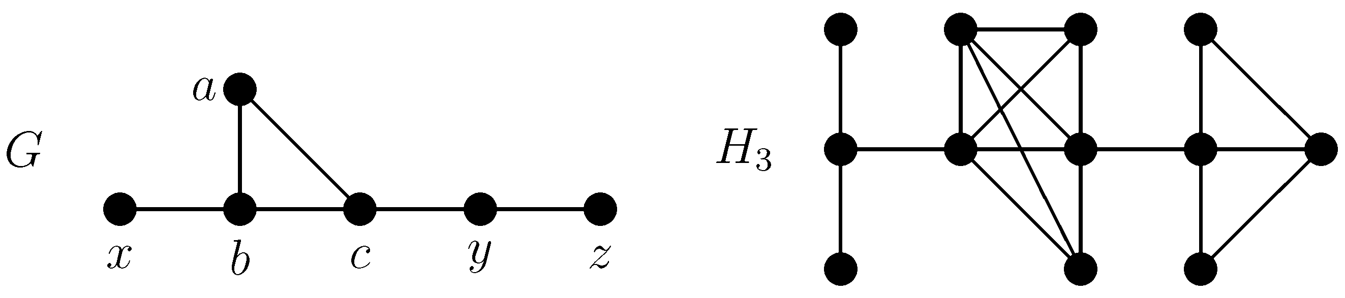
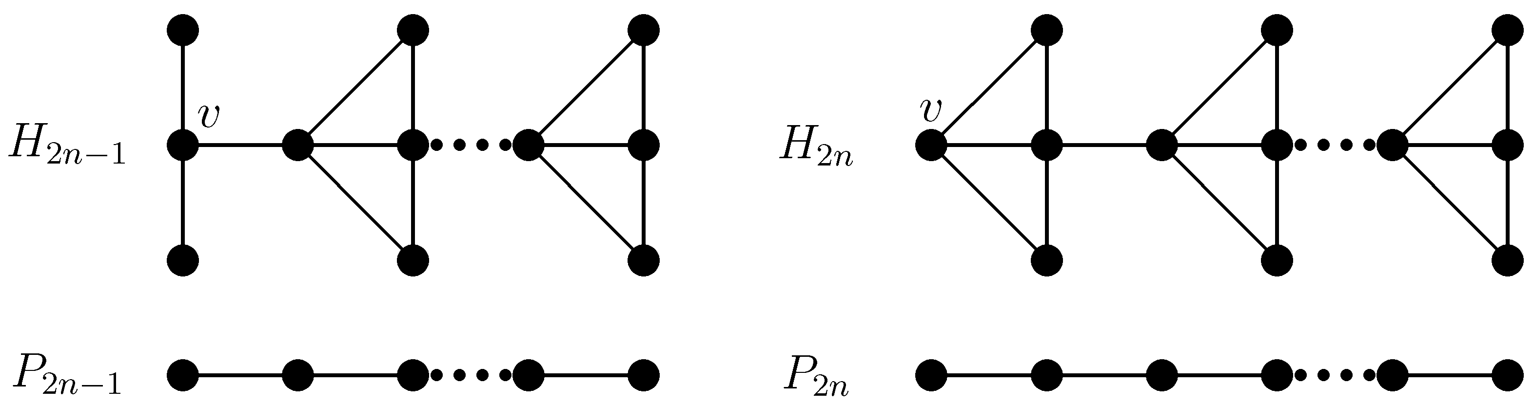
• A cycle cover of a graph G is a spanning graph of G, each connected component of which is a vertex (which we call a vertex-cycle), an edge (which we call an edge-cycle), or a proper cycle. Let $\Gamma$ be a cycle cover of G.

Rule 2. Construct a new graph H from G, denoted by $H=\Gamma \left(G\right)$, as follows: if $C\in \Gamma$ is

(i) a vertex-cycle, say v, then add two vertices and join them to v;

(ii) an edge-cycle, say $uv$, then add two vertices and join them to both u and v;

(iii) a proper cycle, with

$$V\left(C\right)=\{v_i:1\le i\le s\},E\left(C\right)=\{v_i{v}_{i+1}:1\le i\le s-1\}\cup \{v_1{v}_s\},$$

then add s vertices, say $\{w_i:1\le i\le s\}$ and each of them is joined to two consecutive vertices on C, as follows: $w_1$ is joined to $v_s,v_1$, then $w_2$ is joined to $v_1,v_2$, further $w_3$ is joined to $v_2,v_3$, etc.

Figure 6 contains an example, namely, $I(G;x)=1+6x+9x^2+3x^3$, while

$$I(H_2;x)=1+13x+60x^2+125x^3+125x^4+60x^5+13x^6+x^7=$$

$$=\left(1+x\right)\left(1+12x+48x^2+77x^3+48x^4+12x^5+x^6\right).$$

• A clique cover of a graph G is a spanning graph of G, each connected component of which is a clique. Let $\Phi$ be a clique cover of G.

Rule 3. Construct a new graph H from G, denoted by $H=\Phi \left(G\right)$, as follows: for each $Q\in \Phi$, add two non-adjacent vertices and join them to all the vertices of Q.

Figure 7 contains an example, namely, $I(G;x)=1+6x+9x^2+3x^3$, while

$$I(H_3;x)=1+12x+48x^2+77x^3+48x^4+12x^5+x^6.$$

Theorem 2.4.

Let H be the graph obtained from a graph G according to one of the Rules 1, 2 or 3. Then H has a symmetric independence polynomial [17].

Let us remark that $I(H_1;x)={\left(1+x\right)}^6·I(H_3;x)$ and $I(H_2;x)=\left(1+x\right)·I(H_3;x)$, where $H_1,H_2$ and $H_3$ are depicted in Figure 5, Figure 6, and Figure 7, respectively.

2.4. Inequalities and Equalities Following from Theorem 2.4

When inequalities connecting coefficients of the independence polynomial is under consideration, the symmetry mirrors the area, where they are already established. The following results illustrate this idea.

Proposition 2.5.

Let $G=H\circ 2K_1$ be with $\alpha \left(G\right)=\alpha$, and $\left(s_k\right)$ be the coefficients of $I(G;x)$. Then $I(G;x)$ is symmetric, and [22]

$$s_0\le s_1\le \dots \le s_p,forp=⌊(2\alpha +2)/5⌋,while$$

$$s_t\ge \dots \ge s_{\alpha -1}\ge s_{\alpha },fort=⌈(3\alpha -2)/5⌉.$$

Theorem 2.6.

Let H be a graph of order $n\ge 2$, Γ be a cycle cover of H that contains no vertex-cycles, G be obtained by Rule 2, and $\alpha \left(G\right)=\alpha$. Then $I(G;x)$ is symmetric and its coefficients $\left(s_k\right)$ satisfy the subsequent inequalities [22]

$$s_0\le s_1\le \dots \le s_p,forp=⌊(\alpha +1)/3⌋,and$$

$$s_q\ge \dots \ge s_{\alpha -1}\ge s_{\alpha },forq=⌈(2\alpha -1)/3⌉.$$

Let $H_n,n\ge 1$, be the graphs obtained according to Rule 3 from $P_n$, as one can see in Figure 8.

Theorem 2.7.

If $J_n\left(x\right)=I(H_n;x),n\ge 0$, then [23]

(i) $J_0\left(x\right)=1,J_1\left(x\right)=1+3x+x^2$ and $J_n,n\ge 2$, satisfies the following recursive relations:

$$J_{2n}\left(x\right)=J_{2n-1}\left(x\right)+x·J_{2n-2}\left(x\right),n\ge 1,$$

$$J_{2n-1}\left(x\right)={(1+x)}^2·J_{2n-2}\left(x\right)+x·J_{2n-3}\left(x\right),n\ge 2;$$

(ii) $J_n$ is both symmetric and unimodal.

It was conjectured in [23] that $I(H_n;x)$ is log-concave and has only real roots. This conjecture has been resolved as follows.

Theorem 2.8.

Let $n\ge 1$. Then [24]

(i) the independence polynomial of $H_n$ is

$$I(H_n;x)=\prod _{s=1}^{⌊\left(n+1\right)/2⌋}\left(1+4x+x^2+2x·cos\frac{2s\pi }{n+2}\right);$$

(ii) $I(H_n;x)$ has only real zeros, and, therefore, it is log-concave and unimodal.

3. Results

The following lemma goes from the well-known fact that the polynomial $P\left(x\right)$ is symmetric if and only if it equals its reciprocal, i.e.,

$$P\left(x\right)=x^{deg\left(P\right)}·P\left(\frac{1}{x}\right).$$

(1)

Lemma 3.1.

Let $f\left(x\right)$, $g\left(x\right)$ and $h\left(x\right)$ be polynomials satisfying $f\left(x\right)=$$g\left(x\right)·$$h\left(x\right)$. If any two of them are symmetric, then the third is symmetric as well.

For $H=2K_1$, Theorem 1.1 gives

$$I\left(G\circ 2K_1;x\right)={\left(1+x\right)}^{2n}·I\left(G;\frac{x}{{\left(1+x\right)}^2}\right).$$

Since

$$\frac{x}{{\left(1+x\right)}^2}=\frac{\frac{1}{x}}{{\left(1+\frac{1}{x}\right)}^2}anddeg\left(I\left(G\circ 2K_1;x\right)\right)=2n,$$

one can easily see that the polynomial $I\left(G\circ 2K_1;x\right)$ satisfies the identity (1). Thus we conclude with the following.

Theorem 3.2.

For every graph G, the polynomial $I\left(G\circ 2K_1;x\right)$ is symmetric [17].

3.1. Clique Covers Revisited

Lemma 3.3.

If A is a clique in a graph G, then for every graph H

$$I((G,A)\circ H;x)=I{\left(H;x\right)}^{\left|A\right|-1}·I((G,A)+H;x).$$

Proof: 

Let $G_1=(G,A)\circ H$ and $G_2=\left((G,A)+H\right)\cup \left((\left|A\right|-1)H\right)$.

For $S\in Ind\left(G\right)$, let us define the following families of independent sets:

$${\Omega }_S^{G_1}=\{S\cup W:W\subseteq V(G_1-G),S\cup W\in Ind(G_1\},$$

$${\Omega }_S^{G_2}=\{S\cup W:W\subseteq V(G_2-G),S\cup W\in Ind\left(G_2\right)\}.$$

Since A is a clique, it follows that $\left|S\cap A\right|\le 1$.

Case 1. $S\cap A=\varnothing$.

In this case $S\cup W\in {\Omega }_S^{G_1}$ if and only if $S\cup W\in {\Omega }_S^{G_2}$. Hence, for each size $m\ge \left|S\right|$, we get that

$$\left|\{S\cup W\in {\Omega }_S^{G_1}:\left|S\cup W\right|=m\}\right|=\left|\{S\cup W\in {\Omega }_S^{G_2}:\left|S\cup W\right|=m\}\right|.$$

Case 2. $S\cap A=\{a\}$.

Now, every $S\cup W\in {\Omega }_S^{G_1}$ has $W\cap V\left(H\right)=\varnothing$ for exactly one H, namely, the graph H whose vertices are joined to a. Hence, W may contain vertices only from $\left(\left|A\right|-1\right)H$.

On the other hand, each $S\cup W\in {\Omega }_S^{G_2}$ has $W\cap V\left(H\right)=\varnothing$ for the unique H appearing in $(G,A)+H$. Therefore, W may contain vertices only from $\left(\left|A\right|-1\right)H$.

Hence for each positive integer $m\ge \left|S\right|$, we obtain that

$$\left|\{S\cup W\in {\Omega }_S^{G_1}:\left|S\cup W\right|=m\}\right|=\left|\{S\cup W\in {\Omega }_S^{G_2}:\left|S\cup W\right|=m\}\right|.$$

Consequently, one may infer that for each size, the two graphs, $G_1$ and $G_2$, have the same number of independent sets, in other words, $I(G_1;x)=I(G_2;x)$.

Since $G_2=\left((G,A)+H\right)\cup \left((\left|A\right|-1)H\right)$ has $\left|A\right|-1$ disjoint components identical to H, it follows that $I(G_2;x)=I{\left(H;x\right)}^{\left|A\right|-1}·I((G,A)+H;x)$. ◊

Corollary 3.4.

If A is a clique in a graph G, then

$$I((G,A)\circ 2K_1;x)={\left(1+x\right)}^{2\left|A\right|-2}·I((G,A)+2K_1;x).$$

Theorem 3.5.

If G is a graph of order n and Φ is a clique cover, then

$$I(G\circ 2K_1;x)={\left(1+x\right)}^{2n-2\left|\Phi \right|}·I(\Phi \left(G\right);x).$$

Proof: 

Let $\Phi =\left\{A_1,A_2,\dots ,A_q\right\}$. According to Corollary 3.4, each

(a) vertex-clique of $\Phi$ yields ${\left(1+x\right)}^{2-2}=1$ as a factor of $I(G\circ 2K_1;x)$, since a vertex defines a clique of size 1;

(b) edge-clique of $\Phi$ yields ${\left(1+x\right)}^2$ as a factor of $I(G\circ 2K_1;x)$, since an edge defines a clique of size 2 (see Figure 9 as an example);

(c) clique $A_j\in \Phi ,\left|A_j\right|\ge 3$, produces ${\left(1+x\right)}^{2\left|A_j\right|-2}$ as a factor of $I(G\circ 2K_1;x)$ (see Figure 10 as an example).

Since the cliques of $\Phi$ are pairwise vertex disjoint, one can apply Corollary 3.4 to all the q cliques one by one.

Using Corollary 3.4 and the fact that $A_1\cap A_2=\varnothing$, we have

$$I((G,A_1\cup A_2)\circ 2K_1;x)=I(\left(\left((G,A_1)\circ 2K_1\right),A_2\right)\circ 2K_1;x)=$$

$$={\left(1+x\right)}^{2\left|A_2\right|-2}·I(\left(\left((G,A_1)\circ 2K_1\right),A_2\right)+2K_1;x)=$$

$$={\left(1+x\right)}^{2\left|A_2\right|-2}·I(\left(\left((G,A_2)+2K_1\right),A_1\right)\circ 2K_1;x)=$$

$$={\left(1+x\right)}^{2\left(\left|A_1\right|+\left|A_2\right|\right)-2}·I(\left(\left((G,A_2)+2K_1\right),A_1\right)+2K_1;x).$$

Repeating this process with $\left\{A_3,A_4,\dots ,A_q\right\}$, and taking into account that all the cliques of $\Phi$ are pairwise disjoint, we obtain

$$I((G\circ 2K_1;x)=I((G,A_1\cup A_2\cup \dots \cup A_q)\circ 2K_1;x)=$$

$$={\left(1+x\right)}^{2\left(\left|A_1\right|+\left|A_2\right|+\dots +\left|A_q\right|\right)-2q}·I(\left((\left((G,A_1)+2K_1\right),A_2\dots ),A_q\right)+2K_1;x)=$$

$$={\left(1+x\right)}^{2n-2\left|\Phi \right|}·I(\Phi \left(G\right);x),$$

as required. ◊

Lemma 3.1 and Theorem 3.5 imply the following.

Corollary 3.6.

For every clique cover Φ of a graph G, the polynomial $I(\Phi (G);x)$ is symmetric [17].

Clearly, for every $k\le \mu \left(G\right)$ there exists a clique cover containing k non-trivial cliques, namely, edges. Consequently, we obtain the following.

Theorem 3.7.

For every graph G and for each non-negative integer $k\le \mu \left(G\right)$, one can build a graph H, such that: G is a subgraph of H, $I\left(H;x\right)$ is symmetric, and $I\left(G\circ 2K_1;x\right)={\left(1+x\right)}^k·I\left(H;x\right)$.

3.2. Cycle Covers Revisited

Lemma 3.8.

If C is a proper cycle in a graph G, then for every graph H

$$I((G,C)\circ 2H;x)=I{\left(H;x\right)}^{\left|C\right|}·I((G,C)△H;x).$$

Proof: 

Let $C=\left(V\left(C\right),E\left(C\right)\right)$, $q=\left|V\left(C\right)\right|$, $G_1=(G,C)\circ 2H$, and $G_2=\left((G,C)△H\right)\cup \left(qH\right)$.

For an independent set $S\subset V\left(G\right)$, let us denote:

$${\Omega }_S^{G_1}=\{S\cup W:W\subseteq V\left(G_1\right)-V\left(G\right),S\cup W\in Ind\left(G_1\right)\},$$

$${\Omega }_S^{G_2}=\{S\cup W:W\subseteq V\left(G_2\right)-V\left(G\right),S\cup W\in Ind\left(G_2\right)\}.$$

Case 1. $S\cap V\left(C\right)=\varnothing$.

In this case $S\cup W\in {\Omega }_S^{G_1}$ if an only if $S\cup W\in {\Omega }_S^{G_2}$, since W is an arbitrary independent set of $2qH$. Hence, for each size $m\ge \left|S\right|$, we get that

$$\left|\{S\cup W\in {\Omega }_S^{G_1}:\left|S\cup W\right|=m\}\right|=\left|\{S\cup W\in {\Omega }_S^{G_2}:\left|S\cup W\right|=m\}\right|.$$

Case 2. $S\cap V\left(C\right)\ne \varnothing$.

Then, we may assert that

$$\left|{\Omega }_S^{G_1}\right|=\left|\{S\cup W:Wisanindependentsetin2(q-\left|S\cap V\left(C\right)\right|)H\}\right|=\left|{\Omega }_S^{G_2}\right|,$$

since W has to avoid all the “H-neighbors” of the vertices in $S\cap V\left(C\right)$, both in $G_1$ and $G_2$.

Hence, for each positive integer $m\ge \left|S\right|$, we get that

$$\left|\{S\cup W\in {\Omega }_S^{G_1}:\left|S\cup W\right|=m\}\right|=\left|\{S\cup W\in {\Omega }_S^{G_2}:\left|S\cup W\right|=m\}\right|.$$

Consequently, one may infer that for each size, the two graphs, $G_1$ and $G_2$, have the same number of independent sets. In other words, $I(G_1;x)=I(G_2;x)$.

Since $G_2$ has $\left|C\right|$ disjoint components identical to H, it follows that

$$I(G_2;x)={\left(1+x\right)}^{\left|C\right|}·I((G,C)△H;x),$$

as required. ◊

Corollary 3.9.

If C is a proper cycle in a graph G, then

$$I((G,C)\circ 2K_1;x)={\left(1+x\right)}^{\left|C\right|}·I((G,C)△K_1;x).$$

Theorem 3.10.

If G is a graph of order n and Γ is a cycle cover containing k vertex-cycles, then

$$I(G\circ 2K_1;x)={\left(1+x\right)}^{n-k}·I(\Gamma \left(G\right);x).$$

Proof: 

According to Corollaries 3.4 and 3.9, each

(a) vertex-cycle of $\Gamma$ yields ${\left(1+x\right)}^{2-2}=1$ as a factor of $I(G\circ 2K_1;x)$, since each vertex defines a clique of size 1;

(b) edge-cycle of $\Gamma$ yields ${\left(1+x\right)}^2$ as a factor of $I(G\circ 2K_1;x)$, since every edge defines a clique of size 2;

(c) proper cycle $C\in \Gamma$ produces ${\left(1+x\right)}^{\left|C\right|}$ as a factor (see Figure 11 as an example).

Let $\Gamma =\left\{C_j:1\le j\le q\right\}\cup \left\{v_i:1\le i\le k\right\}$ be a cycle cover containing k vertex-cycles, namely, $\left\{v_i:1\le i\le k\right\}$.

Using Corollary 3.9 and the fact that $C_1\cap C_2=\varnothing$, we have

$$I((G,C_1\cup C_2)\circ 2K_1;x)=I(\left(\left((G,C_1)\circ 2K_1\right),C_2\right)\circ 2K_1;x)=$$

$$={\left(1+x\right)}^{\left|C_2\right|}·I(\left(\left((G,C_1)\circ 2K_1\right),C_2\right)△K_1;x)=$$

$$={\left(1+x\right)}^{\left|C_2\right|}·I(\left(\left((G,C_2)△K_1\right),C_1\right)\circ 2K_1;x)=$$

$$={\left(1+x\right)}^{\left|C_1\right|+\left|C_2\right|}·I(\left(\left((G,C_2)△K_1\right),C_1\right)△K_1;x).$$

Repeating this process with $\left\{C_3,C_4,\dots ,C_q\right\}$, and taking into account that all the cycles of $\Gamma$ are pairwise vertex disjoint, we obtain

$$I((G\circ 2K_1;x)=I((G,C_1\cup C_2\cup \dots \cup C_q)\circ 2K_1;x)=$$

$$={\left(1+x\right)}^{\left|C_1\right|+\left|C_2\right|+\dots +\left|C_q\right|}·I(\left((\left((G,C_1)△K_1\right),C_2\dots ),C_q\right)△K_1;x)=$$

$$={\left(1+x\right)}^{n-k}·I(\Gamma \left(G\right);x),$$

as claimed. ◊

Lemma 3.1 and Theorem 3.10 imply the following.

Corollary 3.11.

For every cycle cover Γ of a graph G, the polynomial $I(\Gamma (G);x)$ is symmetric [17].

4. Conclusions

In this paper we have given algebraic proofs for the assertions in Theorem 2.4, due to Stevanović [17]. In addition, we have shown that for every clique cover $\Phi$, and every cycle cover $\Gamma$ of a graph G, the polynomial $I(G\circ 2K_1;x)$ is divisible both by $I(\Phi (G);x)$ and $I(\Gamma (G);x)$.

For instance, the graphs from Figure 12 have:$I(G;x)=1+6x+9x^2+2x^3$, while

$$I(G\circ 2K_1;x)={\left(1+x\right)}^6\left(1+12x+48x^2+76x^3+48x^4+12x^5+x^6\right)=$$

$$={\left(1+x\right)}^5·I(\Gamma \left(G\right);x)={\left(1+x\right)}^6·I(\Phi \left(G\right);x),$$

$$I(\Gamma \left(G\right);x)=1+13x+60x^2+124x^3+124x^4+60x^5+13x^6+x^7,$$

$$I(\Phi \left(G\right);x)=1+12x+48x^2+76x^3+48x^4+12x^5+x^6.$$

The characterization of graphs whose independence polynomials are symmetric is still an open problem [17].

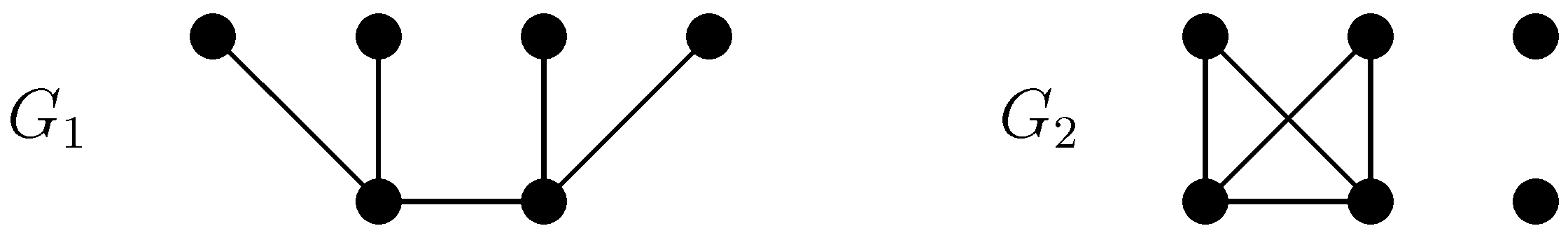
Let us mention that there are non-isomorphic graphs with the same independence polynomial, symmetric or not. For instance, the graphs $G_1$, $G_2$, $G_3$, $G_4$ presented in Figure 13 are non-isomorphic, while

$$I(G_1;x)=I(G_2;x)=1+5x+5x^2,and$$

$$I(G_3;x)=I(G_4;x)=1+6x+10x^2+6x^3+x^4.$$

Recall that a graph having at most two vertices with the same degree is called antiregular [25]. It is known that for every positive integer $n\ge 2$ there is a unique connected antiregular graph of order n, denoted by $A_n$, and a unique non-connected antiregular graph of order n, namely $\overline{A_n}$ [26]. In [27] we showed that the independence polynomial of the antiregular graph $A_n$ is:

$$I(A_{2k-1};x)={\left(1+x\right)}^k+{\left(1+x\right)}^{k-1}-1,and$$

$$I(A_{2k};x)=2·{\left(1+x\right)}^k-1,k\ge 1.$$

Let us mention that $I(A_{2k};x)=I(K_{k,k};x)$ and $I(A_{2k-1};x)=I(K_{k,k-1};x)$, where $K_{m,n}$ denotes the complete bipartite graph on $m+n$ vertices. Notice that the coefficients of the polynomial

$$I(A_{2k};x)=2·{\left(1+x\right)}^k-1=\sum _{j=0}^k{s}_j{x}^j$$

satisfy $s_j=s_{k-j}$ for $1\le j\le ⌊k/2⌋$, while $s_0\ne s_k$, i.e., $I(A_{2k};x)$ is “almost symmetric”.

Problem 4.1.

Characterize graphs whose independence polynomials are almost symmetric.

It is known that the product of a polynomial $P\left(x\right)={\displaystyle \sum _{k=0}^n}{a}_k{x}^k$ and its reciprocal $Q\left(x\right)={\displaystyle \sum _{k=0}^n}{a}_{n-k}{x}^k$ is a symmetric polynomial. Consequently, if $I(G_1;x)$ and $I(G_2;x)$ are reciprocal polynomials, then the independence polynomial of $G_1\cup G_2$ is symmetric, because $I\left(G_1\cup G_2;x\right)=I(G_1;x)·I(G_2;x)$.

Problem 4.2.

Describe families of graphs whose independence polynomials are reciprocal.
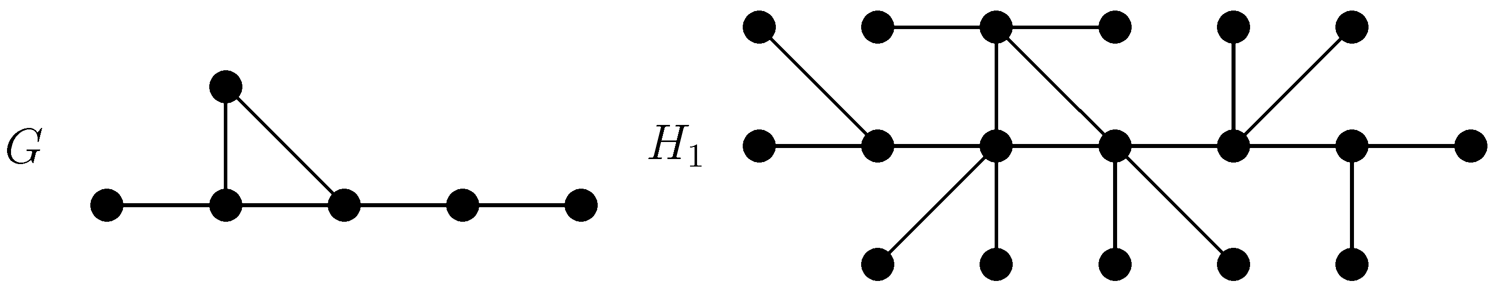