Improving the Performance of Constructed Neural Networks with a Pre-Train Phase

Abstract

A multitude of problems in the contemporary literature are addressed using machine learning models, the most widespread of which are artificial neural networks. Furthermore, in recent years, evolutionary techniques have emerged that identify both the architecture of artificial neural networks and their corresponding parameters. Among these techniques, one can also identify the artificial neural networks being constructed, in which the structure and parameters of the neural network are effectively identified using Grammatical Evolution. In this work, a pre-training stage is introduced in which an artificial neural network with a fixed number of parameters is trained using some optimization technique such as the genetic algorithms used here. The final result of this additional phase is a trained artificial neural network, which is introduced into the genetic population used by Grammatical Evolution in the second phase. In this way, finding the overall minimum of the error function will be significantly accelerated, making the second phase method more efficient. The current work was applied to many classification and regression problems found in the related literature, and it was compared against other methods used for neural network training as well as against the original method used to construct neural networks.

1. Introduction

A machine learning model used widely in classification and regression problems is the artificial neural network [1,2]. Commonly, these models are expressed as functions $N\left(\overrightarrow{x},\overrightarrow{w}\right)$. In this expression, the vector $\overrightarrow{x}$ having dimension d is considered the input vector (pattern) and the vector $\overrightarrow{w}$ is the vector of parameters for the neural network. The learning of these models is obtained by minimizing the training error, which is expressed using the following equation:

$$\mathrm{error}\left(N\left(\overrightarrow{x},\overrightarrow{w}\right)\right)=\sum _{i=1}^M{\left(N\left({\overrightarrow{x}}_i,\overrightarrow{w}\right)-y_i\right)}^2$$

(1)

The set $\left(\overrightarrow{x_i},y_i\right),i=1,\dots ,M$ represents the corresponding training set for the objective problem. In this set, the values $y_i$ define the expected outputs for each pattern $\overrightarrow{x_i}$.

Artificial neural networks have been applied in a wide series of real-world problems, such as image processing [3], time series forecasting [4], credit card analysis [5], problems derived from physics [6], etc. Also, recently they have been applied to flood simulation [7], solar radiation prediction [8], agricultural problems [9], problems appearing in communications [10], mechanical applications [11], etc. During recent years, a wide series of optimization methods has been incorporated to tackle Equation (1), such as the back propagation algorithm [12], the RPROP algorithm [13,14], etc. Furthermore, global optimization methods have been used widely for the training of artificial neural networks, such as the genetic algorithms [15], the particle swarm optimization (PSO) method [16], the simulated annealing method [17], the differential evolution technique [18], the Artificial Bee Colony (ABC) method [19], etc. Moreover, Sexton et al. suggested the usage of the tabu search algorithm for this problem [20], and Zhang et al. introduced a hybrid algorithm that utilizes the PSO method and the back propagation algorithm [21]. Additionally, Zhao et al. introduced a new Cascaded Forward Algorithm for neural network training [22]. Furthermore, a series of parallel computing techniques have been proposed to speed up the training of neural networks [23,24].

However, these techniques face a series of problems. For example, many times, they cannot be freed from local minima of the error function. This will have a direct consequence of low performance of the neural network on the data of the objective problem. Another major problem that appears in the previously mentioned optimization techniques is the overfitting problem, where poor performance is observed when the neural networks are applied to data that was not present during the training process. This problem has been thoroughly studied by many researchers who have proposed some methods to handle this problem. Among these methods, one can detect the weight-sharing method [25], pruning techniques [26,27], early stopping methods [28,29], the weight-decaying procedure [30,31], etc. Additionally, the dynamic construction of the architecture of neural networks was proposed by various researchers as a possible solution for the overfitting problem. For example, genetic algorithms have been proposed to dynamically create the architecture of neural networks [32,33], as well as the PSO method [34]. Recently, Siebel et al. introduced a method based on evolutionary reinforcement learning to obtain the optimal architecture of neural networks [35]. Moreover, Jaafra et al. published a review regarding the usage of reinforcement learning for neural architecture search [36]. Similarly, Pham et al. introduced a novel method based on parameter sharing [37]. Also, the technique of the Stochastic Neural Architecture search was proposed by Xie et al. [38]. Finally, Zhou et al. introduced a Bayesian approach for the same task [39].

Recently, a method that utilizes the Grammatical Evolution [40] to create the architecture of neural networks was proposed. This method can dynamically discover the desired architecture of neural networks, and it can also detect the optimal values for the corresponding parameters [41]. This technique creates various trial structures of artificial neural networks, which, using genetic operators, evolve from generation to generation, aiming to obtain the global minimum of the training error, as provided by Equation (1). This method was applied with success in a series of practical problems. Among them, one can locate chemical problems [42], solutions to differential equations [43], medical problems [44], education problems [45], autism screening [46], etc.

Compared to other techniques for constructing the structure of artificial neural networks, the method guided by Grammatical Evolution has a number of advantages. First of all, this method can generate both the topology and the values for the associated parameters. Furthermore, this method can effectively isolate the features of the dataset that are most important, and furthermore, can retain only those synapses in the neural network that will lead to a reduction in training error. Additionally, this method does not demand prior knowledge of the objective problem and can be applied without any differentiation to both classification problems and regression problems. Furthermore, since a grammar is used to generate the artificial neural network, it is possible for the researcher to explain why one structure may be preferred over others. Finally, since the Grammatical Evolution procedure is used, the method could be faster than others since the Grammatical Evolution utilizes integer-based chromosomes to express valid programs in the underlying grammar.

However, in many cases, training the above model is not efficient and can become trapped in local minima of the error function, which will directly result in poor performance on the problem data. Furthermore, an important factor in the problems addressed by Grammatical Evolution is the initial values that the chromosomes of the genetic population take. If the initialization is not effective, then Grammatical Evolution may take a significant amount of time to find the optimal solution to the problem. Furthermore, in artificial neural networks, an ineffective initialization of the genetic population can lead to the model becoming trapped in local minima of the error function. In this paper, we propose to introduce an additional phase in the artificial neural network construction algorithm. In this phase, an optimization method, such as a genetic algorithm, can train an artificial neural network with a fixed number of parameters. The final result of this additional phase is a trained artificial neural network, which can be introduced into the initial genetic population of Grammatical Evolution. In this way, the evolution of chromosomes will be accelerated and through genetic operators, chromosomes will be produced that will use genetic material from the chromosome introduced from the first phase of the proposed process. The final method was applied to many classification and regression problems, and it was compared against the original neural network construction method; the results seem promising.

Similar works in the field of pre-training neural networks were presented in the related literature. For example, the work of Li et al. focused on the acceleration of the back propagation training algorithm by incorporating an initial weight pre-training [47]. Also, Erhan et al. [48] discussed the role of different pre-training mechanisms for the effectiveness of neural networks. Furthermore, a recent work [49] discusses the effect of pre-training of artificial neural networks for the problem of software fault prediction. Saikia et al. proposed a novel pre-training mechanism [50] to improve the performance of neural networks in the case of regression problems. Moreover, Kroshchanka et al. proposed a method [51] to significantly reduce the number of parameters in neural networks using a pre-training method. Also, Noinongyao et al. introduced a method based on Extreme Learning Machines [52] for the efficient pre-training of artificial neural networks.

The process of constructing neural networks using Grammatical Evolution, as proposed in the article, enables the model to automatically discover a wide range of structures that may incorporate features such as symmetry or asymmetry between connections and layers. This flexibility in designing architectures allows for the representation of both symmetric and asymmetric patterns, which can be important for neural network performance, especially when the problem at hand exhibits intrinsic symmetries in the data or in the relationships among variables. Through the evolutionary process, the proposed approach can result in structures with a higher degree of symmetry in the connections or in the distribution of weights, an aspect that is often associated with improved generalization and stability during training.

Compared to other similar techniques, the present work uses a fixed number of parameters during pre-training, as the goal is not to find a critical number of parameters, but to more effectively initialize the population of the next phase. Furthermore, in the second phase of the algorithm, the optimal architecture for neural networks is found, where the most effective number of parameters will be found. Furthermore, the proposed technique has no dependence on prior knowledge of the data to which it will be applied, and is performed in the same way for both classification and regression problems.

The remainder of this article is divided as follows: in Section 2, the current work and the accompanying genetic algorithm are introduced. In Section 3, the experimental datasets and the series of experiments conducted are listed and discussed thoroughly, followed by Section 4, where some conclusions are discussed.

2. Materials and Methods

The suggested technique consists of two main phases, which are presented here. During the first phase, pre-training takes place, during which a genetic algorithm will attempt to effectively train a neural network with a specific number of weights, which is determined in advance. Of course, any optimization method could be used in the first stage; however, genetic algorithms were chosen because of their adaptability and their ability to search for the global minimum of functions. The final result of the first phase will be a trained artificial neural network, which will be introduced into the genetic population of the Grammatical Evolution of the second phase. This process will result in identifying a range of values in which the optimal value of the training error lies. Furthermore, the optimized neural network that will be introduced into the population will be able to lead to an acceleration of finding the overall minimum of the error function through the application of genetic operators and the exchange of genetic material with other chromosomes of Grammatical Evolution. In the second stage, the Grammatical Evolution method performs the efficient construction of artificial neural networks, in which the chromosomes are arrays of integers that stand for production rules of the given grammar.

2.1. The Pre-Training Phase

During the first phase, an optimization method should be utilized to train a neural network with a fixed number of weights. In the present work, a genetic algorithm was incorporated as the optimization procedure. Genetic algorithms were initially proposed by John Holland [53], and can be considered a global optimization procedure that has been used in a multitude of problems. This method is inspired by biology and it can simulate the evolutionary process through the genetic operations of mutation, natural selection, and crossover [54,55,56]. This method has been applied in cases such as robotics [57], energy problems [58], agriculture problems [59], etc. The neural networks considered here are in the following form:

$$N\left(\overrightarrow{x},\overrightarrow{w}\right)=\sum _{i=1}^H{w}_{(d+2)i-(d+1)}\sigma \left(\sum _{j=1}^d{x}_j{w}_{(d+2)i-(d+1)+j}+w_{(d+2)i}\right)$$

(2)

The constant H defines the number of processing units (weights) of the network and the constant d represents the dimension of the input patterns. The function $\sigma \left(x\right)$ stands for the sigmoid function, expressed as follows:

$$\sigma \left(x\right)={\displaystyle \frac{1}{1+exp\left(-x\right)}}$$

(3)

From Equation (2), it is derived that the number of parameters for the neural network can be computed as follows:

$$n=\left(d+2\right)H$$

(4)

In the present work, the sigmoid function is adopted with one processing layer (hidden layer), due to its approximation capabilities exploited in Hornik’s theorem [60]. According to this theorem, a neural network with a sufficient number of sigmoid units can approximate any given function. The algorithm of the first phase has the following steps:

• Initialization step, where the initialization of the critical parameters for the genetic algorithm is made.
• Fitness Calculation step, where the fitness for each chromosome is performed. Each chromosome is a vector of double precision values used as the parameters of the neural network.
• Application of genetic operators, where the operators of selection, crossover, and mutation are performed.
• Termination check step.

Hence, the steps of the algorithm are as follows:

1.

Initialization step.

(a)

Define as $N_c$ the total number of chromosomes and as $N_g$ the maximum number of generations.

(b)

Define as $p_s$ the selection rate and as $p_m$ the mutation rate.

(c)

Set as $I_w$ the number of initial weights for the neural network.

(d)

Initialize the chromosomes $g_i,i=1,\dots ,N_c$ of the population as randomly produced vectors of double precision numbers. The dimension of each vector is calculated as $n=(d+2)I_w$.

(e)

Set $k=0$, the generation number.

2.

Fitness Calculation step.

(a)

For $i=1,\dots ,N_c$, do

i.

Create a neural network $N_i=N\left(\overrightarrow{x},\overrightarrow{g_i}\right)$ for the chromosome $\overrightarrow{g_i}.$

ii.

Calculate the corresponding fitness value $f_i$ as

$$f_i=\sum _{j=1}^M{\left(N\left({\overrightarrow{x}}_j,\overrightarrow{g_i}\right)-y_j\right)}^2.$$

(5)

(b)

End for

3.

Genetic operations step.

(a)

Selection procedure: Firstly, the chromosomes are sorted with respect to their fitness values. The best $\left(1-p_s\right)\times N_c$ of them are moved without any further change to the next generation. The remaining will be replaced by new chromosomes that will be produced during crossover and mutation.

(b)

Crossover procedure: In this procedure, for each pair of produced chromosomes, defined as $\left(\tilde{z},\tilde{w}\right)$, two parents $(z,w)$ are selected from the current population with the process of tournament selection. The items $\left(\tilde{z},\tilde{w}\right)$ are constructed using the following equations:

$$\begin{array}{ccc}\hfill \widetilde{z_i}& =& a_i{z}_i+\left(1-a_i\right)w_i\hfill \\ \hfill \widetilde{w_i}& =& a_i{w}_i+\left(1-a_i\right)z_i\hfill \end{array}$$

(6)

where $a_i$ are random numbers, with the property $a_i\in [-0.5,1.5]$ [61].

(c)

Mutation procedure: For each element $t_j,j=1,\dots ,n$ of every chromosome $g_i$, a random number $r\in [0,1]$ is selected. The element is changed when $r\le p_m$, according to the scheme:

$$t_j^{\prime }=\left\{\begin{array}{cc}{t}_j+\Delta \left(k,r_j-t_j\right),\hfill & t=0\hfill \\ t_j-\Delta \left(k,t_j-l_j\right),\hfill & t=1\hfill \end{array}\right.$$

(7)

where t are random numbers that have the value 0 or 1. The function $\Delta (k,y)$ has the following definition:

$$\Delta (k,y)=y\left(1-r^{\left(1-{\displaystyle \frac{k}{N_g}}\right)}\right)$$

(8)

4.

Termination check step.

(a)

Set $k=k+1$;

(b)

If $k<N_g$, then go to the Fitness Calculation step, or else terminate.

2.2. The Neural Construction Method

The method that produces artificial neural networks incorporates the Grammatical Evolution procedure. Grammatical Evolution is a genetic algorithm, where the chromosomes are vectors of integers. These integers are rules from a provided Backs–Naur form (BNF) grammar [62] of the target language. The method of Grammatical Evolution was applied in various cases, such as data fitting [63,64], composition of music [65], video games [66,67], energy problems [68], cryptography [69], economics [70], etc. BNF grammars are usually represented as sets $G=\left(N,T,S,P\right)$, where the letters have the following definitions:

• The set N contains the non-terminal symbols of the grammar.
• The set T contains the terminal symbols of the grammar.
• The start symbol of the grammar is denoted as S, with $S\in N$.
• The set P encloses the production rules of the grammar.

The procedure used to create programs in the underlying language initiates from the starting symbol S and using a series of steps, the Grammatical Evolution produces valid programs. This process is performed by the substitution of non-terminal symbols with the right hand of the currently selected production rule. This rule is obtained using the scheme, described subsequently:

• Obtain the next element from the processed chromosome and denote this element as V.
• Select the production rule as follows: Rule = V mod $N_R$, where $N_R$ stands for the total number of production rules for non-terminal symbols, which is currently under processing.

The overall process for the production of producing valid programs using the Grammatical Evolution method is shown graphically in Figure 1.

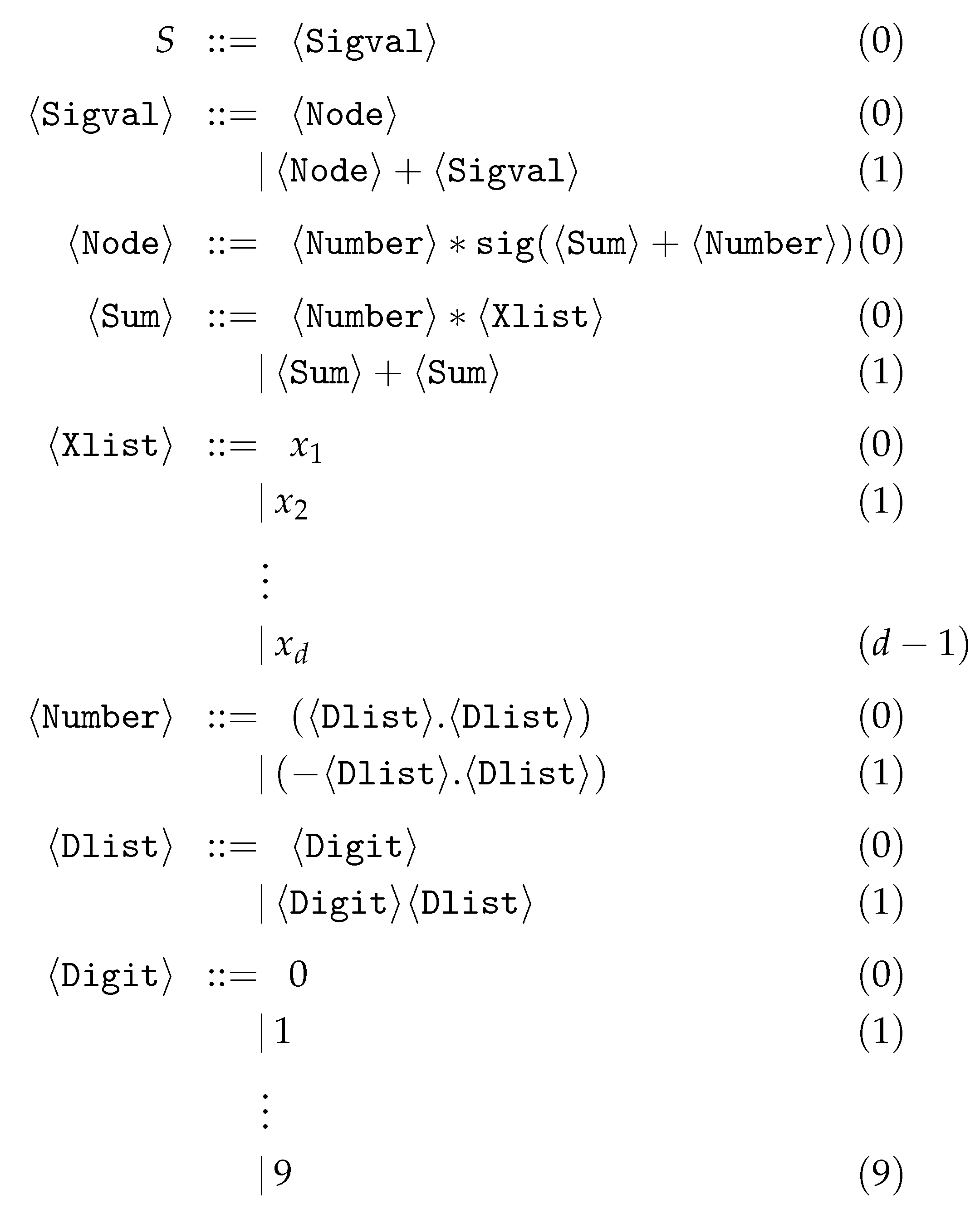
The BNF grammar for the method of neural network construction is shown in Figure 2. The numbers shown in parentheses represent a sequential production rule for the corresponding non-terminal symbol and are used in the process of generating valid programs.

As a working example of the produced neural network, the following form is provided:

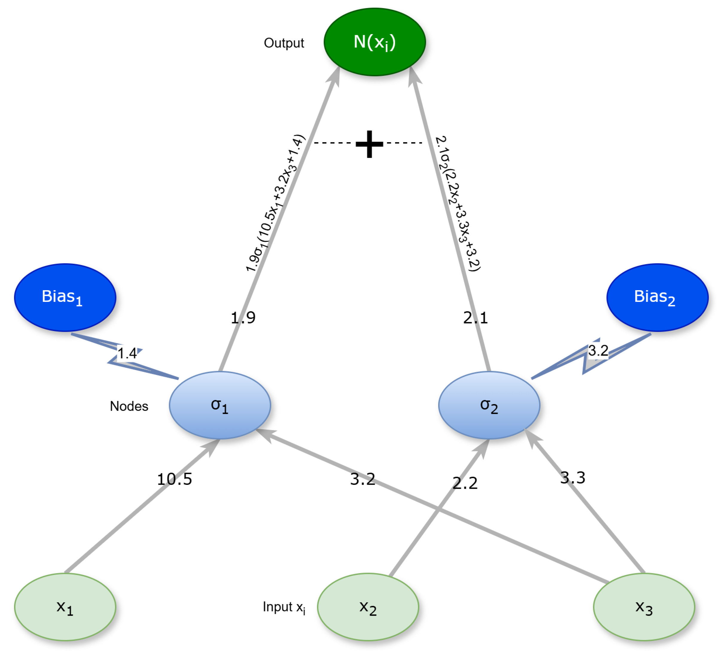
$$N\left(x\right)=1.9\mathrm{sig}\left(10.5x_1+3.2x_3+1.4\right)+2.1\mathrm{sig}\left(2.2x_2-3.3x_3+3.2\right)$$

(9)

This neural network stands for a network with three inputs $\left(x_1,x_2,x_3\right)$. The number of processing units is $H=2$. The network can be shown graphically in Figure 3. The above procedure can produce artificial neural networks with one hidden layer, in which the number of neurons is not predetermined and is decided dynamically during the production of the network. In addition, the connections of the inputs to the neurons are decided dynamically during the construction of the network and therefore it is not mandatory that all inputs are connected to every neuron. Finally, the above grammar can be extended in the future to include artificial neural networks with more than one processing layer.

The main steps of the proposed algorithm are as follows:

1.

Application of first phase.

(a)

Set $I_w$ the number of weights for the first phase.

(b)

Execute the first phase of the current method, as presented in Section 2.1.

(c)

Obtain the chromosome $x^{*}$ of the first phase, having the lowest fitness value.

(d)

Convert the chromosome $x^{*}$ to the corresponding integer chromosome $g^{*}$. This chromosome, with the help of the grammar of Figure 2, can create the chromosome $x^{*}$.

2.

Initialization step.

(a)

Define as $N_c$ the number of chromosomes and as $N_g$ the number of allowed generations.

(b)

Define as $p_s$ the selection rate and as $p_m$ the mutation rate.

(c)

Initialize the chromosomes $g_i,i=1,\dots ,N_c$ as sets of positive random integers.

(d)

Insert the chromosome $g^{*}$ to a random position $r_i\in \left[1,N_c\right]$.

(e)

Set as $k=0$ the generation counter.

3.

Fitness Calculation step.

(a)

For  $i=1,\dots ,N_c$  do

i.

Create the constructed neural network $N_i\left(\overrightarrow{x},\overrightarrow{w}\right)$ for the corresponding chromosome $g_i$ using the grammar of Figure 2.

ii.

Calculate the fitness value $f_i$ as

$$f_i=\sum _{j=1}^M{\left(N\left({\overrightarrow{x}}_j,\overrightarrow{w}\right)-y_j\right)}^2$$

(10)

(b)

End for

4.

Application of genetic operations.

(a)

Application of selection procedure: The chromosomes are sorted according to their fitness values and the best $\left(1-p_s\right)\times N_c$ of them are transferred to the next generation. The remaining chromosomes will be substituted by new chromosomes produced by crossover and mutation.

(b)

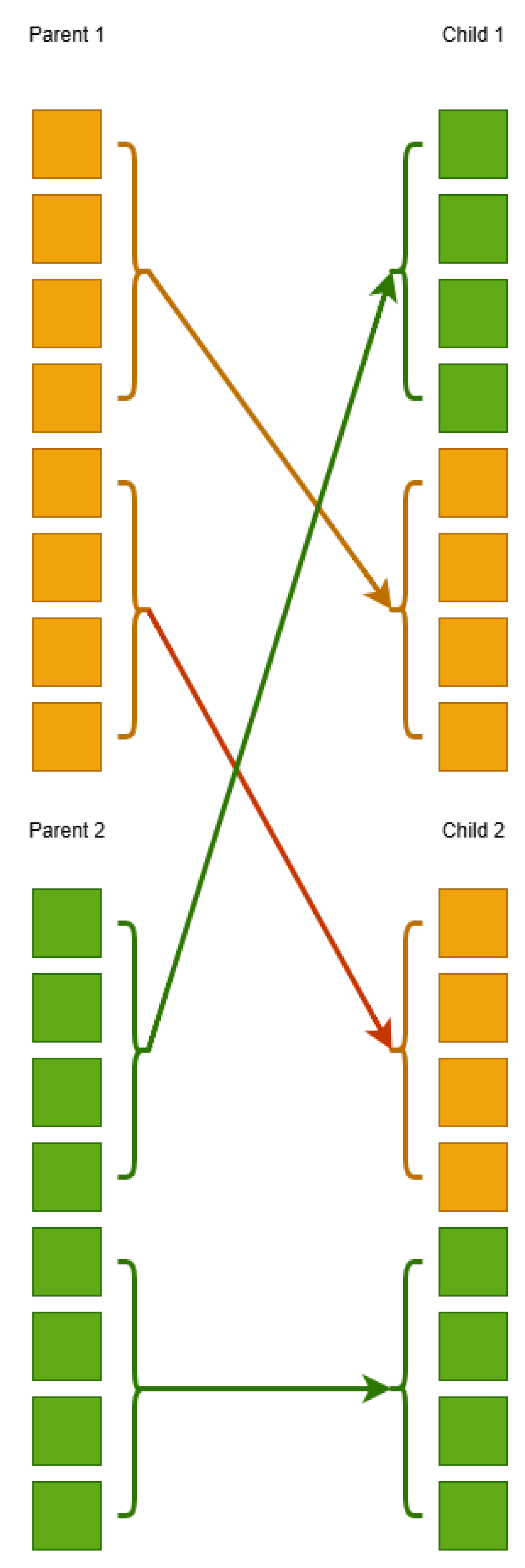
Application of crossover procedure: During crossover, for each pair of new chromosomes defined as $\left(\tilde{z},\tilde{w}\right)$, two parents $(z,w)$ are selected from the current population using tournament selection. The new offspring are produced using one-point crossover. An example process for the one-point crossover is depicted graphically in Figure 4.

(c)

Application of mutation procedure: For every element of each chromosome, a random number $r\in [0,1]$ is selected. The corresponding element is altered randomly when $r\le p_m$.

5.

Termination check step.

(a)

Set $k=k+1$.

(b)

If $k<N_g$, then go to the Fitness Calculation step, or else go to the Testing step.

6.

Testing step.

(a)

Obtain the chromosome $g^{*}$ having the lowest fitness value.

(b)

Create the neural network $N^{*}\left(\overrightarrow{x},\overrightarrow{w}\right)$ for the chromosome $g^{*}$ with the grammar depicted in Figure 2.

(c)

Apply the neural network $N^{*}\left(\overrightarrow{x},\overrightarrow{w}\right)$ to the test data of the objective problem and report the results.

3. Results

The validation of the current work was performed with the assistance of a series of classification and regression datasets, which can be accessed freely from the Internet from the following sites:

• The UCI database, https://archive.ics.uci.edu/ (accessed on 9 September 2025) [71].
• The Keel website, https://sci2s.ugr.es/keel/datasets.php (accessed on 9 September 2025) [72].
• The Statlib URL https://lib.stat.cmu.edu/datasets/index (accessed on 9 September 2025).

3.1. Experimental Datasets

The classification datasets used in the conducted experiments are the following:

• Appendictis dataset [73].
• Alcohol, used in experiments related to alcohol consumption [74].
• Australian, which is a dataset produced from various bank transactions [75].
• Balance dataset [76], produced from various psychological experiments.
• Cleveland, a medical dataset which was discussed in a series of papers [77,78].
• Circular dataset, which was produced artificially with two distinct classes.
• Dermatology, which is related to dermatology problems [79].
• Ecoli, a dataset regarding protein problems [80].
• Glass, a dataset that contains measurements from glass component analysis.
• Haberman, a medical dataset used for the detection of breast cancer.
• Hayes–Roth dataset [81].
• Heart, which is used for the detection of heart diseases [82].
• HeartAttack, used in a variety of heart diseases.
• Housevotes, a dataset which contains measurement forms related to congressional voting in the USA [83].
• Ionosphere, a commonly used dataset regarding measurements from the ionosphere [84,85].
• Liverdisorder, a medical dataset that was studied thoroughly in a series of papers [86,87].
• Lymography dataset [88].
• Mammographic, which is related to breast cancer detection [89].
• Parkinsons, which is related to the detection of Parkinson’s disease [90,91].
• Pima, related to the detection of diabetes [92].
• Phoneme, a dataset that contains sound measurements.
• Popfailures, which is related to measurements regarding climate [93].
• Regions2, a dataset used for the detection of liver problems [94].
• Saheart, which is a medical dataset concerning heart diseases [95].
• Segment dataset [96].
• Statheart, a dataset related to the detection of heart diseases.
• Spiral, an artificial dataset with two classes.
• Student, which is a dataset regarding experiments in schools [97].
• Transfusion dataset [98].
• Wdbc, a medical dataset regarding breast cancer [99,100].
• Wine, a dataset regarding measurements of the quality of wines [101,102].
• EEG, a dataset related to EEG measurements [103,104], and the following cases were used from this dataset: Z_F_S, ZO_NF_S, ZONF_S and Z_O_N_F_S.
• Zoo, which is related to the classification of animals in some predefined categories [105].

Also, the following list of regression datasets was used in the conducted experiments:

• Abalone, related to the detection of the age of abalones [106].
• Airfoil, a dataset provided by NASA [107].
• Auto, regarding fuel consumption in cars.
• BK, used to predict the points scored by basketball players.
• BL, a dataset regarding some electricity experiments.
• Baseball, used to estimate the income of baseball players.
• Concrete, related to measurements from civil engineering [108].
• DEE, a dataset used to estimate the electricity prices.
• Friedman dataset [109].
• FY, related to fruit flies.
• HO, a dataset founded in the STATLIB repository.
• Housing, a dataset used for the prediction of the price of houses [110].
• Laser, which contains measurements from various physics experiments.
• LW, a dataset regarding the weight of babes.
• Mortgage, a dataset that contains measurements from the economy of the USA.
• PL dataset, located in the STALIB repository.
• Plastic, a dataset related to problem in plastics.
• Quake, a dataset that contains measurements from earthquakes.
• SN, a dataset used in trellising and pruning.
• Stock, related to the prices of stocks.
• Treasury, an economic dataset.

3.2. Experiments

The code used in the current work was coded in the C++ language, and the freely available Optimus environment [111] was used. All the experiments were repeated 30 times, using a different seed for the random generator in every run. For the validation of the experimental results, the well-known procedure of ten-fold cross-validation was incorporated. For the classification datasets, the average classification error is reported, as calculated using the following formula:

$$E_C\left(N\left(\overrightarrow{x},\overrightarrow{w}\right)\right)=100\times {\displaystyle \frac{{\sum }_{i=1}^N\left(\mathrm{class}\left(N\left(\overrightarrow{x_i},\overrightarrow{w}\right)\right)-y_i\right)}{N}}$$

(11)

The set T represents the test set and it is defined as $T=\left(x_i,y_i\right),i=1,\dots ,N$. Likewise, for the regression datasets, the average regression error is reported and is computed using the following expression:

$$E_R\left(N\left(\overrightarrow{x},\overrightarrow{w}\right)\right)={\displaystyle \frac{{\sum }_{i=1}^N{\left(N\left(\overrightarrow{x_i},\overrightarrow{w}\right)-y_i\right)}^2}{N}}$$

(12)

The values for the experimental settings are depicted in

Table 1. The values for the parameters of the PROPOSED method.

Parameter	Purpose	Value
$N_c$	Chromosomes	500
$N_g$	Maximum number of allowed generations	500
$p_s$	Selection rate	0.1
$p_m$	Mutation rate	0.05
$I_w$	Number of weights for the first phase	10

. The parameter values have been set so that there is a compromise between the efficiency and speed of the methodologies used when performing the experiments. The following notation is used in the experimental tables:

• The column DATASET represents the objective problem.
• The column ADAM denotes the results from the training of a neural network using the ADAM optimizer [112]. The number of processing nodes was set to $H=10$.
• The column BFGS represents the results obtained by the training of a neural network with $H=10$ processing nodes using the BFGS variant of Powell [113].
• The column GENETIC stands for the results obtained by the training of a neural network with $H=10$ processing nodes using Genetic Algorithm with the same parameter set, as provided in Table 1.
• The column RBF describes the incorporation of a Radial Basis Function (RBF) network [114,115], with $H=10$ hidden nodes.
• The column NNC represents the results obtained by the incorporation of the original neural construction method.
• The column NEAT represents the usage of the NEAT method (NeuroEvolution of Augmenting Topologies) [116].
• The column PRUNE stands for the usage of the OBS pruning method [117], provided by the Fast Compressed Neural Networks library [118].
• The column PROPOSED shows the results obtained by the application of the proposed method.
• The row AVERAGE depicts the average classification or regression error for all datasets in the corresponding table.

In

Table 2. Experimental results using a variety of machine learning methods for the classification datasets.

DATASET	ADAM	BFGS	GENETIC	RBF	NEAT	PRUNE	NNC	PROPOSED
APPENDICITIS	16.50%	18.00%	24.40%	12.23%	17.20%	15.97%	14.40%	16.30%
ALCOHOL	57.78%	41.50%	39.57%	49.32%	66.80%	15.75%	37.72%	20.21%
AUSTRALIAN	35.65%	38.13%	32.21%	34.89%	31.98%	43.66%	14.46%	14.68%
BALANCE	12.27%	8.64%	8.97%	33.53%	23.14%	9.00%	23.65%	7.26%
CLEVELAND	67.55%	77.55%	51.60%	67.10%	53.44%	51.48%	50.93%	44.90%
CIRCULAR	19.95%	6.08%	5.99%	5.98%	35.18%	12.76%	12.66%	4.22%
DERMATOLOGY	26.14%	52.92%	30.58%	62.34%	32.43%	9.02%	21.54%	5.92%
ECOLI	64.43%	69.52%	54.67%	59.48%	43.44%	60.32%	49.88%	44.79%
GLASS	61.38%	54.67%	52.86%	50.46%	55.71%	66.19%	56.09%	49.43%
HABERMAN	29.00%	29.34%	28.66%	25.10%	24.04%	29.38%	27.53%	28.57%
HAYES–ROTH	59.70%	37.33%	56.18%	64.36%	50.15%	45.44%	33.69%	30.77%
HEART	38.53%	39.44%	28.34%	31.20%	39.27%	27.21%	15.67%	17.85%
HEARTATTACK	45.55%	46.67%	29.03%	29.00%	32.34%	29.26%	20.87%	20.67%
HOUSEVOTES	7.48%	7.13%	6.62%	6.13%	10.89%	5.81%	3.17%	7.39%
IONOSPHERE	16.64%	15.29%	15.14%	16.22%	19.67%	11.32%	11.29%	13.14%
LIVERDISORDER	41.53%	42.59%	31.11%	30.84%	30.67%	49.72%	32.35%	33.38%
LYMOGRAPHY	39.79%	35.43%	28.42%	25.50%	33.70%	22.02%	25.29%	25.14%
MAMMOGRAPHIC	46.25%	17.24%	19.88%	21.38%	22.85%	38.10%	17.62%	17.77%
PARKINSONS	24.06%	27.58%	18.05%	17.41%	18.56%	22.12%	12.74%	14.05%
PIMA	34.85%	35.59%	32.19%	25.78%	34.51%	35.08%	28.07%	24.34%
POPFAILURES	5.18%	5.24%	5.94%	7.04%	7.05%	4.79%	6.98%	7.19%
REGIONS2	29.85%	36.28%	29.39%	38.29%	33.23%	34.26%	26.18%	25.00%
SAHEART	34.04%	37.48%	34.86%	32.19%	34.51%	37.70%	29.80%	30.11%
SEGMENT	49.75%	68.97%	57.72%	59.68%	66.72%	60.40%	53.50%	9.59%
SPIRAL	47.67%	47.99%	48.66%	44.87%	48.66%	50.38%	48.01%	41.25%
STATHEART	44.04%	39.65%	27.25%	31.36%	44.36%	28.37%	18.08%	20.26%
STUDENT	5.13%	7.14%	5.61%	5.49%	10.20%	10.84%	6.70%	7.18%
TRANSFUSION	25.68%	25.84%	24.87%	26.41%	24.87%	29.35%	25.77%	23.59%
WDBC	35.35%	29.91%	8.56%	7.27%	12.88%	15.48%	7.36%	3.73%
WINE	29.40%	59.71%	19.20%	31.41%	25.43%	16.62%	13.59%	10.41%
Z_F_S	47.81%	39.37%	10.73%	13.16%	38.41%	17.91%	14.53%	6.60%
Z_O_N_F_S	78.79%	65.67%	64.81%	48.70%	77.08%	71.29%	48.62%	49.66%
ZO_NF_S	47.43%	43.04%	21.54%	9.02%	43.75%	15.57%	13.54%	3.94%
ZONF_S	11.99%	15.62%	4.36%	4.03%	5.44%	3.27%	2.64%	2.60%
ZOO	14.13%	10.70%	9.50%	21.93%	20.27%	8.53%	8.70%	5.10%
AVERAGE	35.75%	35.24%	27.64%	29.97%	33.40%	28.70%	23.82%	19.63%

, classification error rates are presented for a variety of machine learning models applied to the series of classification datasets. The values indicate error percentages, meaning that lower values correspond to better model performance on each dataset. The final row shows the average error rate for each model, serving as a general indicator of overall performance across all datasets. Based on the analysis of the average errors, it becomes evident that the current method achieves the lowest average error rate, with a value of 19.63%. This suggests that it generally outperforms the other methods. It is followed by the NNC model, with an average error of 24.79%, which also demonstrates a significantly lower error compared to traditional approaches such as ADAM, BFGS, and GENETIC, whose average error rates are 36.45%, 35.71%, and 28.25%, respectively. The PRUNE method also performs relatively well, with a mean error of 27.94%. On an individual dataset level, the PROPOSED method achieves the best performance (i.e., the lowest error) in a considerable number of cases, such as in the CIRCULAR, DERMATOLOGY, SEGMENT, Z_F_S, ZO_NF_S, ZONF_S, and ZOO datasets, where it records the smallest error among all methods. Furthermore, in many of these cases, the performance gap between the PROPOSED method and the others is quite significant, indicating the method’s stability and reliability across various data conditions and structures. Some models, including GENETIC, RBF, and NEAT, tend to show relatively high errors in several datasets, which may be due to issues such as overfitting, poor adaptation to non-linear relationships, or generally weaker generalization capabilities. In contrast, the NNC and PRUNE models demonstrate more consistent behavior, while the PROPOSED method maintains not only the lowest overall error, but also reliable performance across a wide range of problem types. In summary, the statistical analysis of classification error rates confirms the superiority of the PROPOSED method over the others, both in terms of average performance and the number of datasets in which it excels. This conclusion is further supported by the observation that the PROPOSED method achieves the best results in the majority of datasets, often with significantly lower error rates. Such superiority may be attributed to better adaptability to data characteristics, effective avoidance of overfitting, and, more broadly, a more flexible or advanced algorithmic architecture.

Table 3. Experimental results using a variety of machine learning methods on the regression datasets.

DATASET	ADAM	BFGS	GENETIC	RBF	NEAT	PRUNE	NNC	PROPOSED
ABALONE	4.30	5.69	7.17	7.37	9.88	7.88	5.08	4.41
AIRFOIL	0.005	0.003	0.003	0.27	0.067	0.002	0.004	0.001
AUTO	70.84	60.97	12.18	17.87	56.06	75.59	17.13	11.73
BK	0.0252	0.28	0.027	0.02	0.15	0.027	0.10	0.058
BL	0.622	2.55	5.74	0.013	0.05	0.027	1.19	0.13
BASEBALL	77.90	119.63	103.60	93.02	100.39	94.50	61.57	60.42
CONCRETE	0.078	0.066	0.0099	0.011	0.081	0.0077	0.008	0.004
DEE	0.63	2.36	1.013	0.17	1.512	1.08	0.26	0.26
FRIEDMAN	22.90	1.263	1.249	7.23	19.35	8.69	6.29	1.25
FY	0.038	0.19	0.65	0.041	0.08	0.042	0.11	0.13
HO	0.035	0.62	2.78	0.03	0.169	0.03	0.015	0.073
HOUSING	80.99	97.38	43.26	57.68	56.49	52.25	25.47	15.96
LASER	0.03	0.015	0.59	0.03	0.084	0.007	0.025	0.004
LW	0.028	2.98	1.90	0.03	0.03	0.02	0.011	0.32
MORTGAGE	9.24	8.23	2.41	1.45	14.11	12.96	0.30	0.15
PL	0.117	0.29	0.29	2.118	0.09	0.032	0.047	0.021
PLASTIC	11.71	20.32	2.791	8.62	20.77	17.33	4.20	2.15
QUAKE	0.07	0.42	0.04	0.07	0.298	0.04	0.96	0.061
SN	0.026	0.40	2.95	0.027	0.174	0.032	0.026	0.10
STOCK	180.89	302.43	3.88	12.23	12.23	39.08	8.92	3.96
TREASURY	11.16	9.91	2.93	2.02	15.52	13.76	0.43	0.25
AVERAGE	22.46	30.29	9.31	10.02	14.65	15.40	6.29	4.83

presents the application of various machine learning methods on regression datasets. In this table, columns represent different algorithms, and rows correspond to datasets. The numerical values shown are absolute errors, indicating the magnitude of deviation from the actual values. Therefore, smaller values signify higher prediction accuracy for the corresponding model. The last row reports the average error for each method across all datasets, offering a general measure of overall performance. According to the overall results, the PROPOSED method exhibits the lowest average error value at 4.83, indicating high accuracy and better overall behavior compared to the other approaches. The second-best performing model is NNC, with an average error of 6.29, which also stands out from the traditional methods. On the other hand, ADAM and BFGS show significantly higher error rates, at 22.46 and 30.29, respectively, suggesting that these methods may not adapt well to the specific characteristics of the regression problems evaluated. At the individual dataset level, the PROPOSED method achieves notably low error values across multiple datasets, including AIRFOIL, CONCRETE, LASER, PL, PLASTIC, and STOCK, outperforming other algorithms by a considerable margin. Its consistent performance across such diverse problems suggests that it is a flexible and reliable approach. Furthermore, the fact that it also performs strongly on more complex datasets with high variability in error—such as AUTO and BASEBALL—strengthens the impression that the method adapts effectively to varying data structures. By comparison, algorithms such as GENETIC and RBF exhibit less stable behavior, showing good performance in some datasets but poor results in others, resulting in a higher overall average error. The PRUNE method, although not a traditional algorithm, shows moderate performance overall, while NEAT does not appear to stand out in any particular dataset and also maintains a relatively high average error. In conclusion, the analysis indicates that the PROPOSED method clearly excels in predictive accuracy, both on average and across a large number of individual datasets. Its ability to minimize error across different types of problems makes it a particularly promising option for regression tasks involving heterogeneous data.

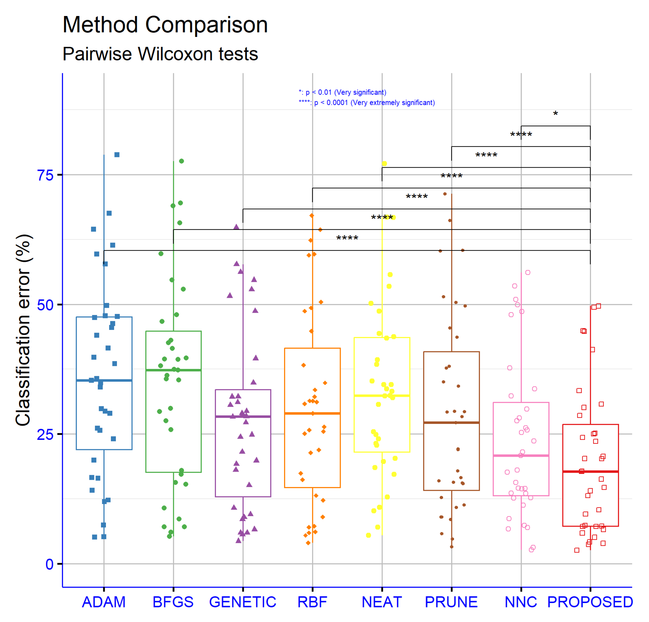
To determine the significance levels of the experimental results presented in the classification dataset tables, statistical analyses were conducted. Exclusively, the non-parametric, paired Wilcoxon signed-rank test was used to assess the statistical significance of the differences between the PROPOSED method and the other methods, as well as for hyperparameter comparisons in both classification and regression tasks. These analyses were based on the critical parameter “p”, which is used to assess the statistical significance of performance differences between models. As shown in Figure 5, the differences in performance between the PROPOSED model and all other models, namely ADAM, BFGS, GENETIC, RBF, NEAT, and PRUNE, are extremely statistically significant with p < 0.0001. This indicates, with a high level of confidence, that the PROPOSED model outperforms the rest in classification accuracy. Even the comparison with NNC, which is the model with the closest average performance, showed a statistically significant difference with p < 0.05. This confirms that the superiority of the PROPOSED model is not due to random variation, but is statistically sound and consistent. Therefore, the PROPOSED model can be confidently considered the best choice among the evaluated models for classification tasks, based on the experimental data and corresponding statistical analysis.

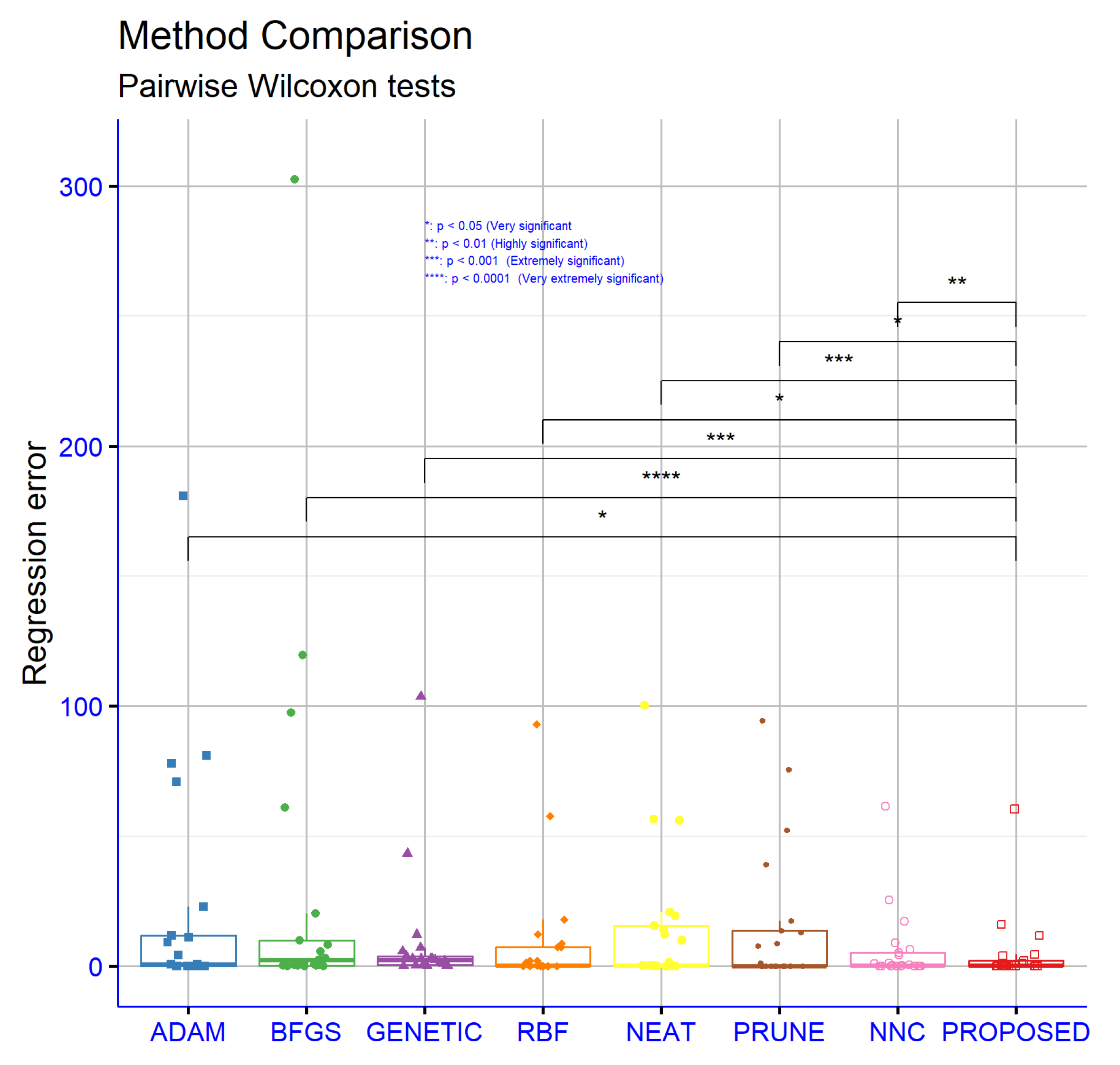
From the analysis of the results presented in Figure 6, it is evident that the performance difference between the PROPOSED model and BFGS is extremely significant (p < 0.0001), clearly indicating the superiority of the PROPOSED model. Similarly, the comparisons with GENETIC and NEAT show very high statistical significance (p < 0.001), confirming that the PROPOSED model achieves clearly better results. The difference with NNC, though smaller, remains significant (p < 0.01), showing that even in comparison with one of the best-performing alternative models, the PROPOSED model still outperforms. The differences with ADAM, RBF, and PRUNE are statistically significant at the p < 0.05 level, suggesting a noteworthy advantage of the PROPOSED model in these cases as well, albeit with a lower confidence level. Overall, the statistical analysis of the regression dataset results confirms the overall superiority of the PROPOSED model, not only in terms of average prediction accuracy, but also in the consistency of its performance compared to the alternative approaches.

3.3. Experiments with the Weight Factor $I_w$

An additional experiment was conducted, where the initial weight parameter $I_w$, used in the first phase of the current work was altered from 2 to 10. The purpose of this experiment is to determine the stability of the proposed procedure to changes in this critical parameter.

Table 4. Experimental results using the PROPOSED method and different values for the parameter $I_w$. The method was applied to the classification datasets.

DATASET	${\mathit{I}}_{\mathit{w}}=2$	${\mathit{I}}_{\mathit{w}}=3$	${\mathit{I}}_{\mathit{w}}=5$	${\mathit{I}}_{\mathit{w}}=10$
APPENDICITIS	15.03%	15.67%	17.93%	16.30%
ALCOHOL	21.11%	25.63%	22.20%	20.21%
AUSTRALIAN	13.93%	14.01%	14.06%	14.68%
BALANCE	8.71%	8.91%	8.61%	7.26%
CLEVELAND	42.09%	42.24%	43.60%	44.90%
CIRCULAR	14.71%	6.93%	4.11%	4.22%
DERMATOLOGY	9.09%	6.78%	6.78%	5.92%
ECOLI	48.21%	56.21%	50.12%	44.79%
GLASS	54.76%	54.51%	52.40%	49.43%
HABERMAN	30.31%	29.11%	28.82%	28.57%
HAYES–ROTH	27.74%	31.31%	28.90%	30.77%
HEART	15.00%	15.32%	15.69%	17.85%
HEARTATTACK	18.61%	18.72%	19.17%	20.67%
HOUSEVOTES	5.80%	6.83%	6.88%	7.39%
IONOSPHERE	11.58%	15.16%	15.88%	13.14%
LIVERDISORDER	31.12%	31.70%	31.89%	33.38%
LYMOGRAPHY	21.76%	23.83%	26.84%	25.14%
MAMMOGRAPHIC	16.33%	16.49%	16.72%	17.77%
PARKINSONS	13.33%	13.47%	13.97%	14.05%
PIMA	23.57%	23.82%	23.76%	24.34%
POPFAILURES	4.98%	5.51%	7.11%	7.19%
REGIONS2	24.63%	25.10%	25.58%	25.00%
SAHEART	29.41%	29.27%	30.48%	30.11%
SEGMENT	39.10%	24.74%	15.17%	9.59%
SPIRAL	47.10%	43.25%	42.66%	41.25%
STATHEART	18.06%	19.12%	19.01%	20.26%
STUDENT	3.73%	4.00%	4.54%	7.18%
TRANSFUSION	24.81%	24.38%	24.28%	23.59%
WDBC	3.25%	3.40%	3.60%	3.73%
WINE	9.08%	8.94%	9.37%	10.41%
Z_F_S	5.43%	5.53%	5.89%	6.60%
Z_O_N_F_S	48.60%	49.67%	48.79%	49.66%
ZO_NF_S	3.30%	3.11%	3.52%	3.94%
ZONF_S	1.97%	2.06%	2.24%	2.60%
ZOO	5.13%	6.57%	5.63%	5.10%
AVERAGE	20.32%	20.33%	19.89%	19.63%

presents the results from the application of the PROPOSED method on various classification datasets, using four distinct values of the parameter $I_w$ (initialization factor): 2, 3, 5, and 10. The recorded values correspond to error percentages for each dataset, while the last row of the table includes the average error rate for each parameter value. Analyzing the data, it is observed that the value $I_w=10$ exhibits the lowest average error rate (19.63%), followed by $I_w=5$ (19.89%). The values $I_w=2$ and $I_w=3$ have slightly higher averages, 20.32% and 20.33%, respectively. The difference between the averages is relatively small, a fact suggesting that the parameter $I_w$ does not dramatically affect the model’s performance; however, the gradual decrease in average error with increasing parameter value may indicate a trend of improvement.

In individual datasets, small variations are observed depending on the setting. In some cases, such as SEGMENT and CIRCULAR, increasing the parameter value leads to noticeably better results. For example, in SEGMENT, the error rate decreases from 39.10% for $I_w=2$ to only 9.59% for $I_w=10$. A similar improvement is observed in CIRCULAR, where the error decreases from 14.71% to 4.22%. Conversely, in other datasets, the variation in values is smaller or negligible, and in some cases, such as ECOLI and CLEVELAND, higher $I_w$ values lead to slightly increased error. Overall, the statistical analysis shows that although no statistically significant differences are observed between the different parameter values, in accordance with the p-values from previous analyses, there is nevertheless an indication that higher values of $I_w$, such as 10, are associated with slightly improved average performance and better results in certain datasets. This trend may be interpreted as an indication that a higher initialization factor might allow the model to start from more favorable learning conditions, particularly in datasets with greater complexity. However, because the variation is not systematic across all datasets, the selection of the $I_w$ value should be conducted carefully and in relation to the characteristics of each specific problem.

In

Table 5. Experimental results using the PROPOSED method and different values for the parameter $I_w$, which is used for the number of parameters for the initial phase of the method. The experiments were performed on the regression datasets.

DATASET	${\mathit{I}}_{\mathit{w}}=2$	${\mathit{I}}_{\mathit{w}}=3$	${\mathit{I}}_{\mathit{w}}=5$	${\mathit{I}}_{\mathit{w}}=10$
ABALONE	4.49	4.40	4.33	4.41
AIRFOIL	0.002	0.002	0.002	0.001
AUTO	17.16	16.14	14.55	11.73
BK	0.13	0.18	0.12	0.058
BL	0.005	0.19	0.14	0.13
BASEBALL	59.05	52.43	54.83	60.42
CONCRETE	0.005	0.004	0.003	0.004
DEE	0.27	0.26	0.26	0.26
FRIEDMAN	6.49	4.56	1.96	1.25
FY	0.07	0.12	0.26	0.13
HO	0.03	0.02	0.08	0.073
HOUSING	27.19	25.53	21.47	15.96
LASER	0.003	0.003	0.003	0.004
LW	0.11	0.09	0.14	0.32
MORTGAGE	0.25	0.25	0.19	0.15
PL	0.022	0.021	0.021	0.021
PLASTIC	3.17	2.33	2.18	2.15
QUAKE	0.043	0.045	0.049	0.061
SN	0.03	0.04	0.06	0.10
STOCK	8.79	8.15	8.91	3.96
TREASURY	0.39	0.40	0.38	0.25
AVERAGE	6.08	5.48	5.24	4.83

, a general trend of decreasing average error is observed as the value of the initialization factor $I_w$ increases. The average drops from 6.08 (for $I_w=2$) to 5.48 ($I_w=3$), 5.24 ($I_w=5$), and finally 4.83 ($I_w=10$). This sequential decrease suggests that higher values of $I_w$ tend to improve the model’s overall performance. However, the effect is not uniform across all datasets. In some cases, the improvement is striking: in AUTO, the error decreases from 17.16 ($I_w=2$) to 11.73 ($I_w=10$), in HOUSING, it reduces from 27.19 to 15.96, and in FRIEDMAN, the most noticeable improvement is recorded from 6.49 to 1.25. Additionally, in STOCK, a significant drop from 8.79 to 3.96 is observed. Conversely, in some datasets, performance deteriorates with increasing $I_w$: in BASEBALL, the error increases from 59.05 ($I_w=2$) to 60.42 ($I_w=10$), and in LW, from 0.11 to 0.32. In other datasets, such as AIRFOIL, LASER, and PL, differences are minimal and practically negligible, with values remaining very close for all $I_w$ parameters. For example, in AIRFOIL, all values are around 0.002, while in PL, the difference between values is merely 0.001. This heterogeneity in the response of different datasets underscores that the optimal value of $I_w$ depends significantly on the specific characteristics of each problem. Despite the general improving trend with higher $I_w$ values, notable exceptions like BASEBALL and LW confirm that there is no global optimal setting suitable for all regression problems.

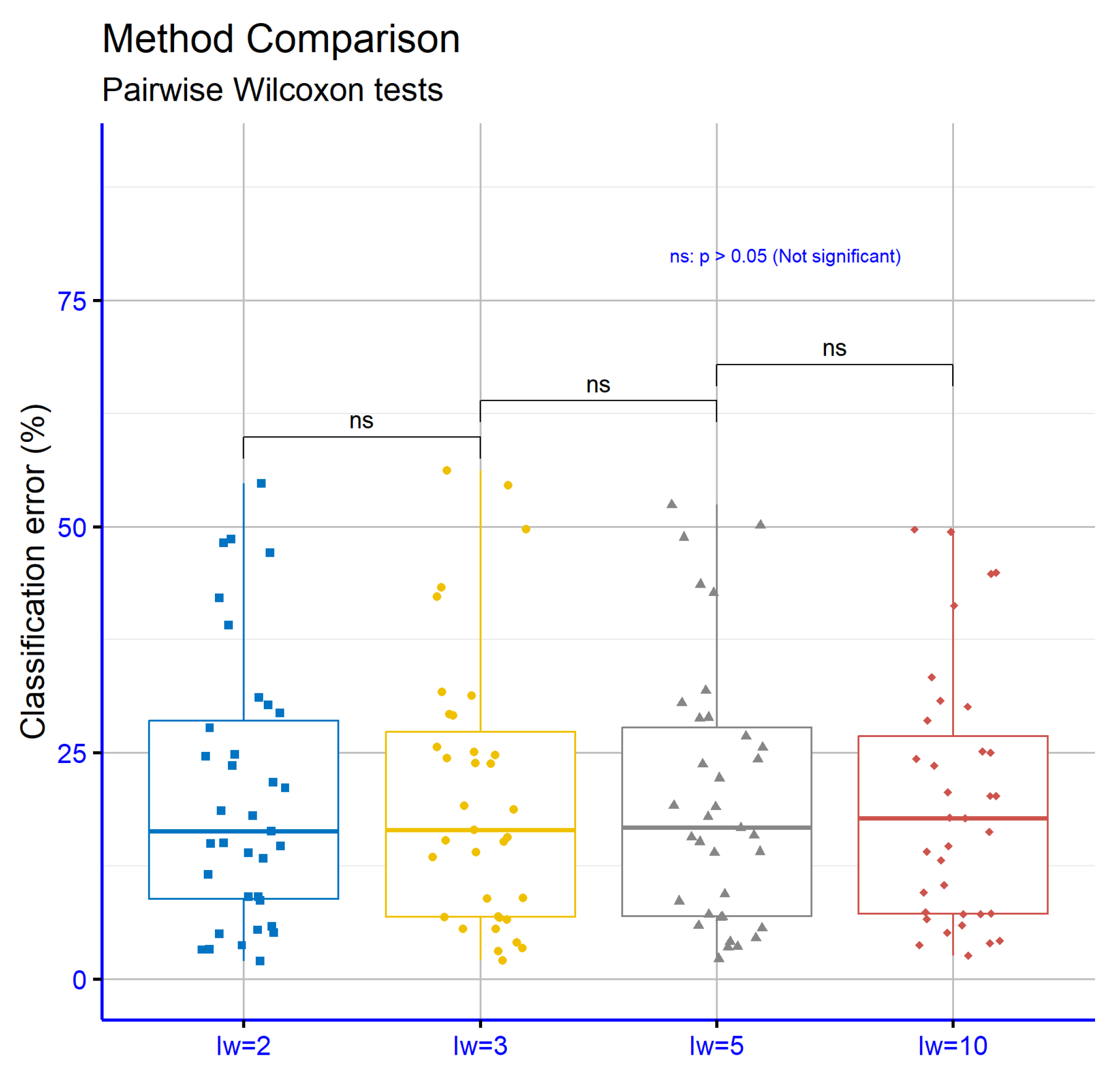
Figure 7 presents the significance levels for the comparison of different values of the $I_w$ (initial weights) parameter in classification datasets. The comparisons include the pairs $I_w=2$ vs. $I_w=3$, $I_w=3$ vs. $I_w=5$, and $I_w=5$ vs. $I_w=10$. In all cases, the p-values are greater than 0.05, indicating that the differences between the respective settings are not statistically significant. This implies that changes in the $I_w$ parameter across these specific values do not substantially change the performance of the model in classification tasks.

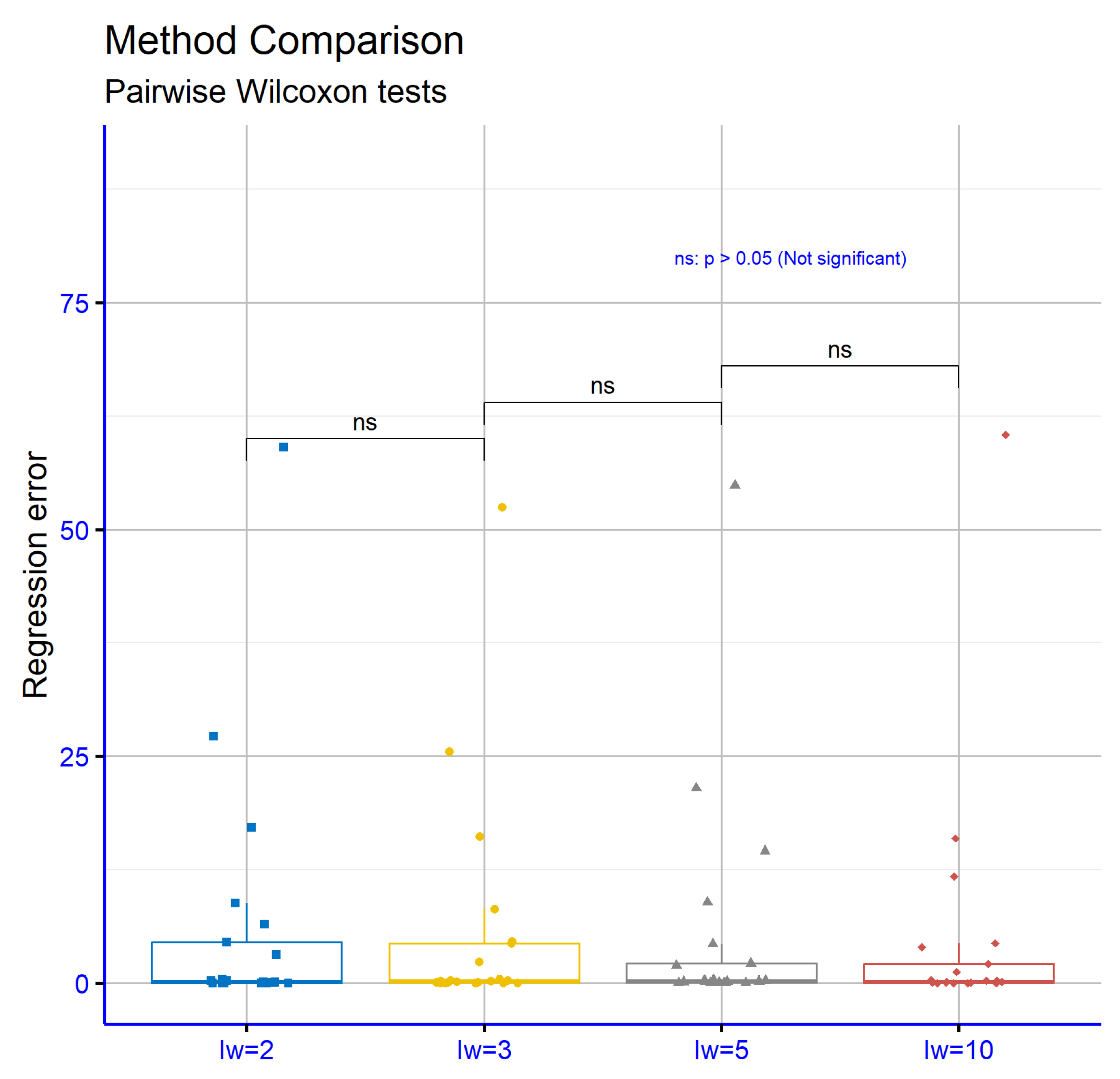
In Figure 8, the statistical evaluation focuses on how different initial weight settings ($I_w$) affect performance in regression tasks. The comparisons between the values $I_w=2$, $I_w=3$, $I_w=5$, and $I_w=10$ revealed no significant variations, as all corresponding p-values were found to be greater than 0.05. This outcome suggests that altering the $I_w$ parameter within this range does not lead to measurable differences in the models’ predictive behavior. The results imply that model accuracy remains stable regardless of these specific $I_w$ configurations in regression scenarios.

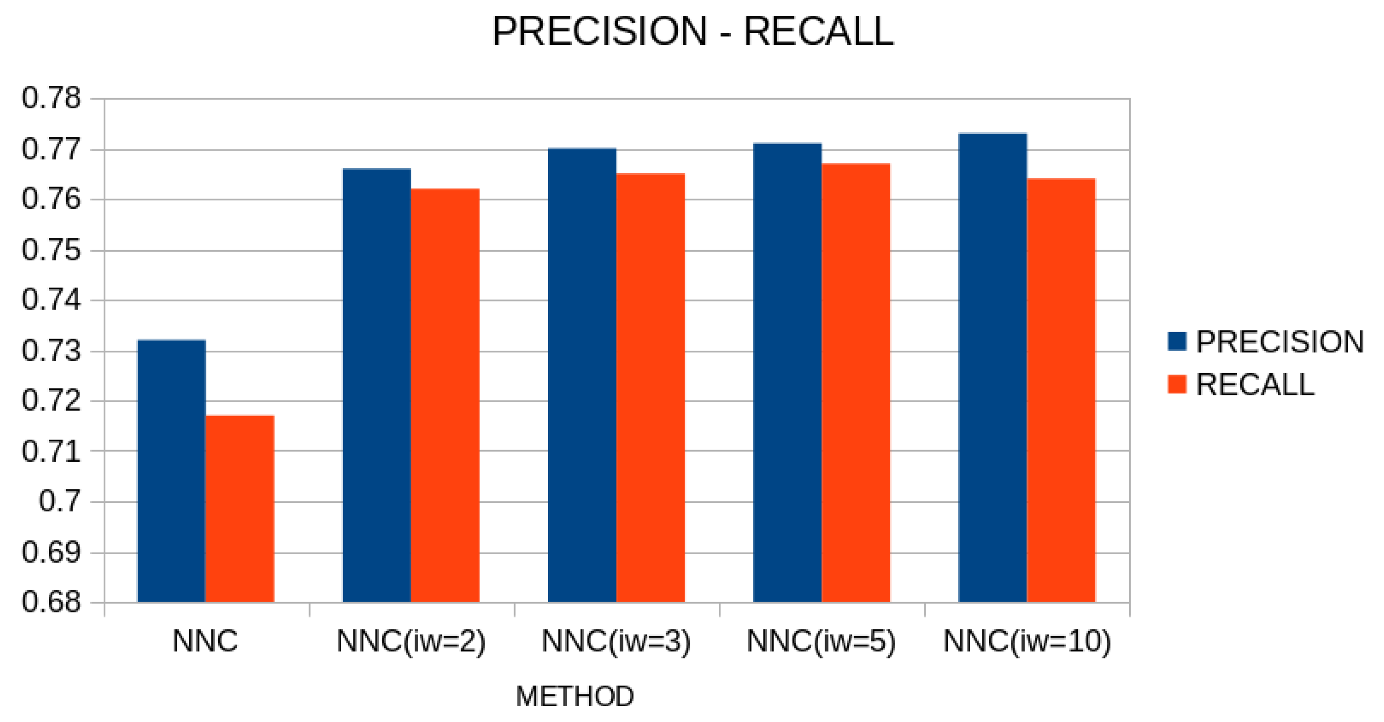
A comparison in terms of precision and recall between the original neural network construction method and the proposed one is outlined in Figure 9.

As can be clearly seen from this figure, the proposed technique significantly improves the performance of the artificial neural network construction method on classification data, achieving high rates of correct data classification.

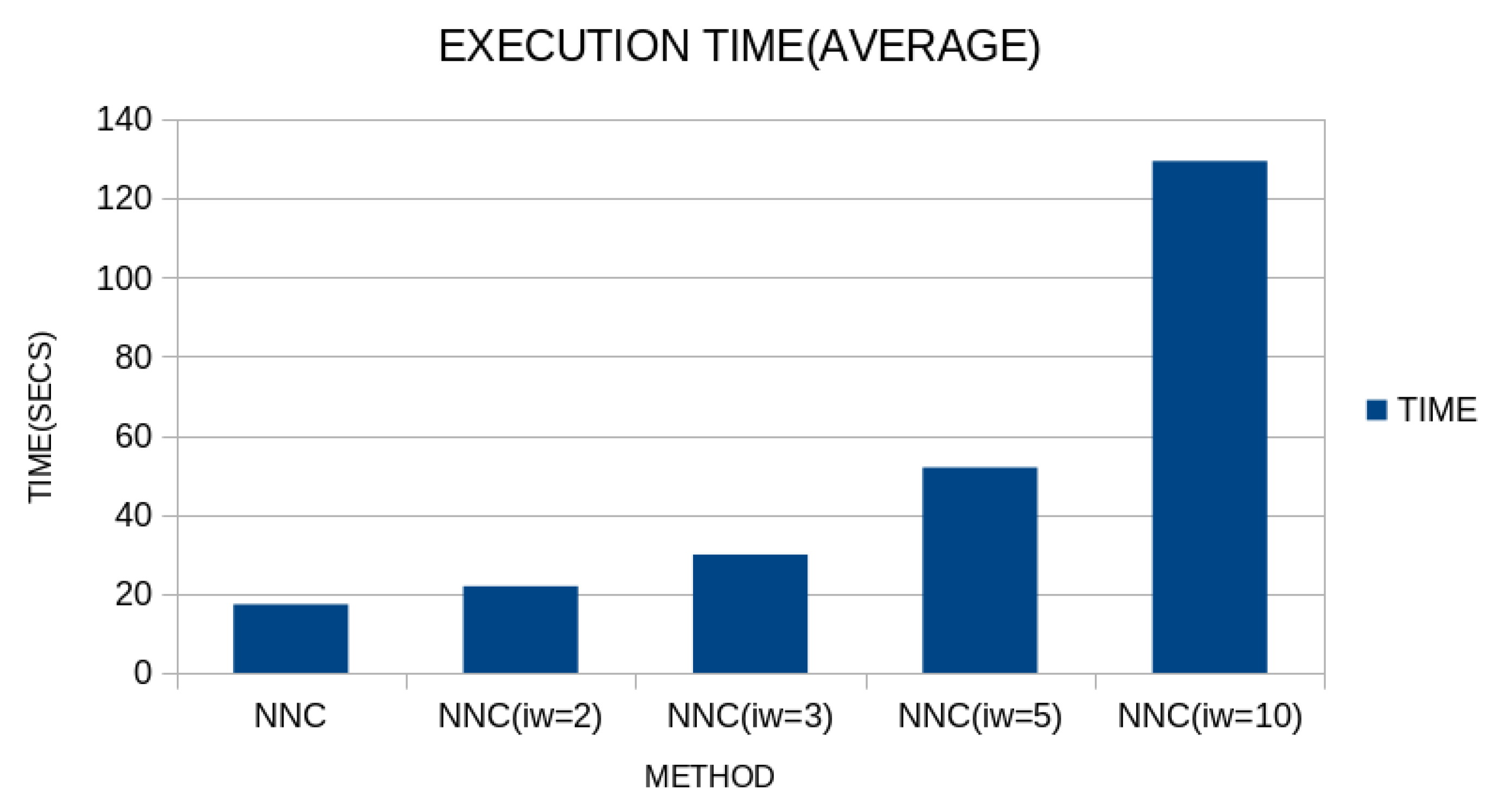
Although the proposed technique appears to be more efficient than the original one, the addition of the first processing phase results in a significant increase in execution time, as also demonstrated in Figure 10.

It is clear that there is a significant increase in execution time, as more units are added to the initial neural network of the first phase, and in fact, this time increases significantly between the values $I_w=5$ and $I_w=10$.

3.4. Some Real-World Examples

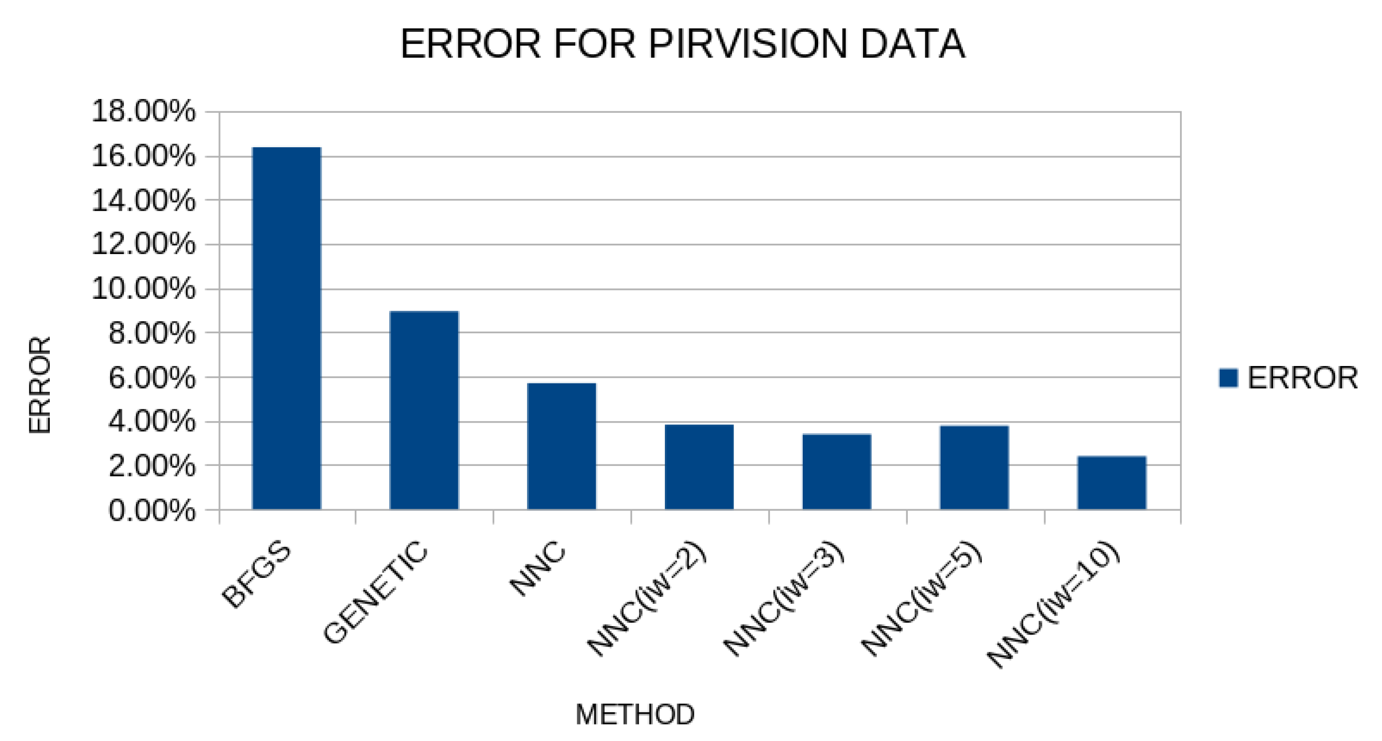
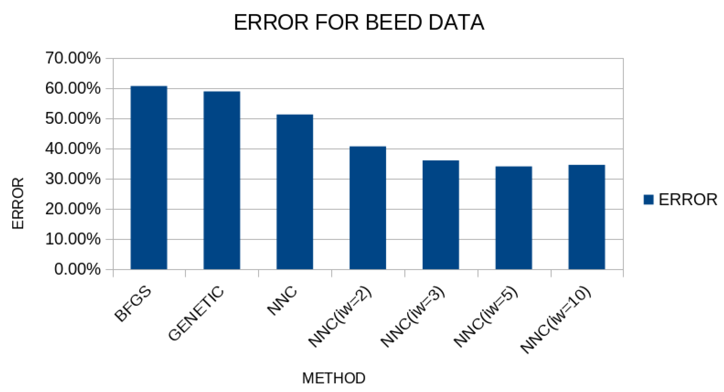
Many real-world examples consider the PIRvision dataset, initially discussed in 2023 [119], and the Beed dataset, presented in the work of Banu [120]. The dataset contains 15302 patterns, and the dimension of each pattern is 59. The Beed dataset (Bangalore EEG Epilepsy Dataset) is a comprehensive EEG collection for epileptic seizure detection and classification, containing 8000 patterns, and each pattern has 16 features. In the conducted experiments, the following methods were used:

• BFGS, which defines the usage of the BFGS method to train a neural network with $H=10$ processing nodes.
• GENETIC, which is used to represent a genetic algorithm used to train a neural network with $H=10$ processing nodes.
• NNC, which represents the initial neural network construction method.
• The PROPOSED method with the following values for $I_w$ parameter: $I_w=2$, $I_w=3,I_w=5$, and $I_w=10$.

For the validation of the results, the method of ten-fold cross-validation was used and the results are shown in Figure 11.

As is evident from the specific results, the artificial neural network construction technique significantly outperforms the others, and in fact, the proposed procedure significantly improves the results, especially in the case where the parameter $I_w$ takes the value 10, where the average classification error reaches approximately 2%.

The results for the BEED dataset are outlined in Figure 12.

And in this case, the PROPOSED method reduces the classification error in comparison to a simple genetic algorithm or compared to the original method of constructing artificial neural networks.

3.5. Experiments with the Number of Chromosomes $N_c$

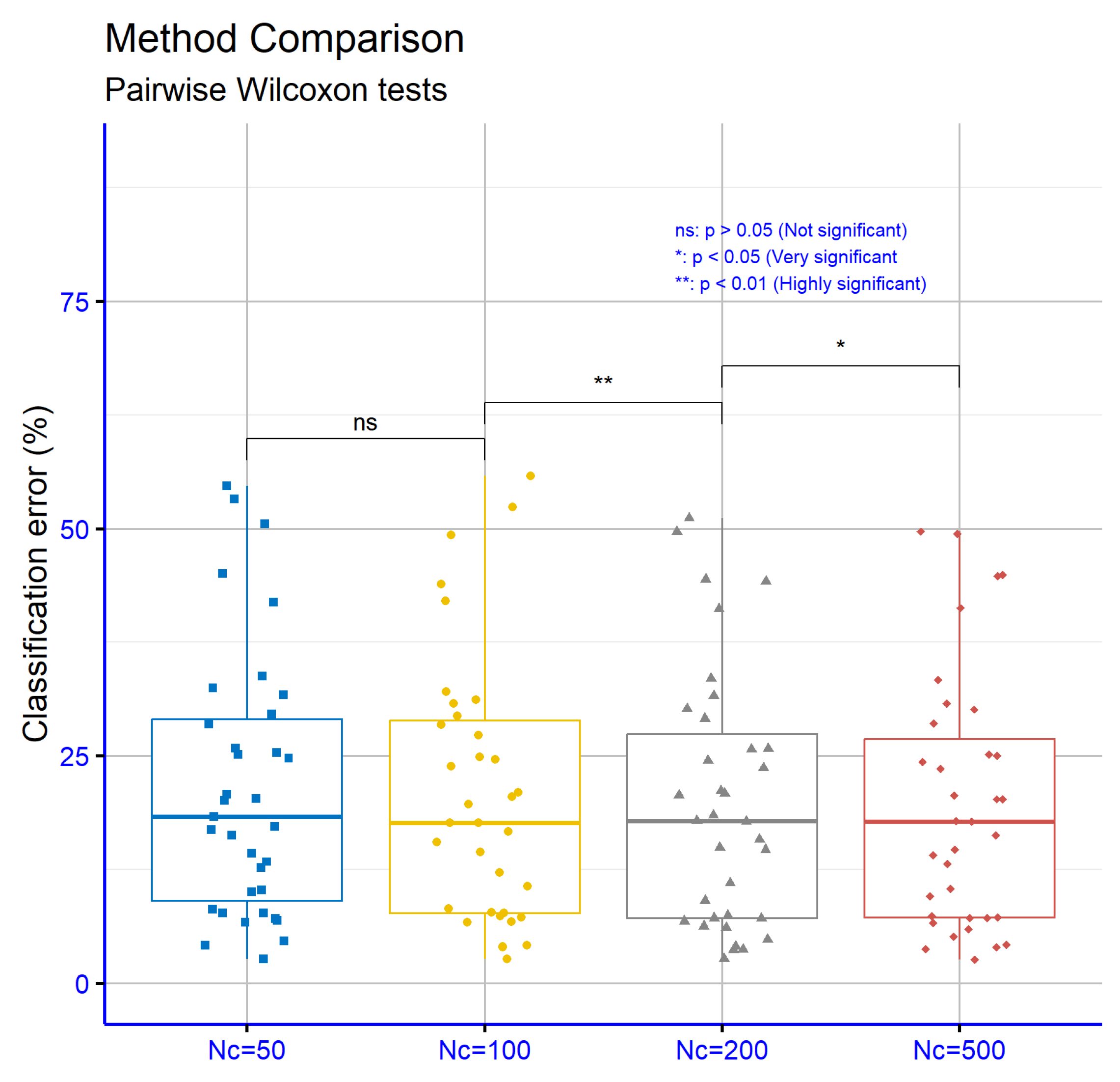
Additionally, another experiment was conducted using the current work and a range of values for the critical parameter $N_c$, which represents the number of used chromosomes.

Table 6. Experimental results for the classification datasets, using the proposed method and a series of values for the parameter $N_c$.

DATASET	${\mathit{N}}_{\mathit{c}}=50$	${\mathit{N}}_{\mathit{c}}=100$	${\mathit{N}}_{\mathit{c}}=200$	${\mathit{N}}_{\mathit{c}}=500$
APPENDICITIS	20.80%	20.50%	18.50%	16.30%
ALCOHOL	24.74%	28.47%	20.85%	20.21%
AUSTRALIAN	14.26%	14.40%	14.68%	14.68%
BALANCE	7.71%	7.79%	6.82%	7.26%
CLEVELAND	45.03%	43.86%	44.42%	44.90%
CIRCULAR	4.67%	4.02%	4.08%	4.22%
DERMATOLOGY	10.26%	7.71%	6.11%	5.92%
ECOLI	54.70%	49.30%	44.18%	44.79%
GLASS	50.48%	52.33%	49.62%	49.43%
HABERMAN	29.57%	29.40%	29.10%	28.57%
HAYES–ROTH	32.47%	31.16%	31.62%	30.77%
HEART	18.34%	17.63%	17.85%	17.85%
HEARTATTACK	20.07%	21.00%	20.67%	20.67%
HOUSEVOTES	7.09%	8.22%	7.44%	7.39%
IONOSPHERE	16.91%	16.69%	15.79%	13.14%
LIVERDISORDER	33.77%	32.06%	33.50%	33.38%
LYMOGRAPHY	25.36%	24.86%	25.72%	25.14%
MAMMOGRAPHIC	17.23%	17.67%	17.81%	17.77%
PARKINSONS	13.37%	15.53%	14.95%	14.05%
PIMA	25.82%	24.64%	24.50%	24.34%
POPFAILURES	7.74%	7.39%	7.17%	7.19%
REGIONS2	28.53%	27.29%	25.78%	25.00%
SAHEART	31.70%	30.74%	30.15%	30.11%
SEGMENT	16.29%	12.16%	9.08%	9.59%
SPIRAL	41.93%	42.04%	41.19%	41.25%
STATHEART	20.30%	19.67%	21.15%	20.26%
STUDENT	6.73%	7.25%	7.13%	7.18%
TRANSFUSION	25.15%	23.86%	23.69%	23.59%
WDBC	4.14%	4.16%	3.73%	3.73%
WINE	10.06%	10.65%	11.00%	10.41%
Z_F_S	12.73%	6.70%	6.27%	6.60%
Z_O_N_F_S	53.26%	55.78%	51.14%	49.66%
ZO_NF_S	8.12%	3.98%	3.66%	3.94%
ZONF_S	2.70%	2.64%	2.66%	2.60%
ZOO	6.90%	6.80%	4.80%	5.10%
AVERAGE	21.40%	20.81%	19.91%	19.63%

presents the classification error rates of the proposed machine learning method across various datasets, for four distinct values of $N_c$, which corresponds to the number of chromosomes used in the evolutionary process. It is observed that, in a large proportion of datasets, an increase in $N_c$ is accompanied by a reduction in the error rate, indicating that a greater diversity of initial solutions can lead to better final performance. In certain datasets, such as DERMATOLOGY, ECOLI, SEGMENT, and Z_F_S, the improvement is particularly evident at higher $N_c$ values, whereas in others, such as AUSTRALIAN, HEART, and MAMMOGRAPHIC, the change is small or nonexistent, suggesting that performance in these cases is less sensitive to an increase in the number of chromosomes. There are also instances where increasing $N_c$ does not lead to improvement but rather to a slight increase in error, as in GLASS and CIRCULAR, a phenomenon that may be due to overfitting or random variation in performance. The mean percentage error gradually decreases from 21.40% for $N_c=50$ to 19.63% for $N_c=500$, confirming the general trend of improvement with increasing $N_c$, although the benefit from very large values appears to diminish, possibly indicating saturation in the model’s ability to exploit the additional diversity. Overall, the statistical picture shows that increasing the number of chromosomes contributes to reducing the error, but the degree of benefit depends on the characteristics of each dataset.

Table 7. Experimental results for the regression datasets, using the proposed method and a series of values for the parameter $N_c$.

DATASET	${\mathit{N}}_{\mathit{c}}=50$	${\mathit{N}}_{\mathit{c}}=100$	${\mathit{N}}_{\mathit{c}}=200$	${\mathit{N}}_{\mathit{c}}=500$
ABALONE	4.35	4.38	4.34	4.41
AIRFOIL	0.001	0.001	0.001	0.001
AUTO	18.99	16.57	11.25	11.73
BK	0.044	0.344	0.14	0.058
BL	0.81	0.77	0.45	0.13
BASEBALL	62.38	63.29	68.56	60.42
CONCRETE	0.004	0.004	0.004	0.004
DEE	0.33	0.33	0.28	0.26
FRIEDMAN	1.24	1.24	1.23	1.25
FY	0.33	0.21	0.26	0.13
HO	0.046	0.10	0.22	0.073
HOUSING	21.71	22.05	15.97	15.96
LASER	0.003	0.003	0.003	0.004
LW	0.30	0.31	0.68	0.32
MORTGAGE	0.36	0.20	0.16	0.15
PL	0.027	0.021	0.021	0.021
PLASTIC	2.92	2.18	2.11	2.15
QUAKE	0.076	0.065	0.059	0.061
SN	0.30	0.19	0.14	0.10
STOCK	6.69	5.23	4.66	3.96
TREASURY	0.56	0.53	0.30	0.25
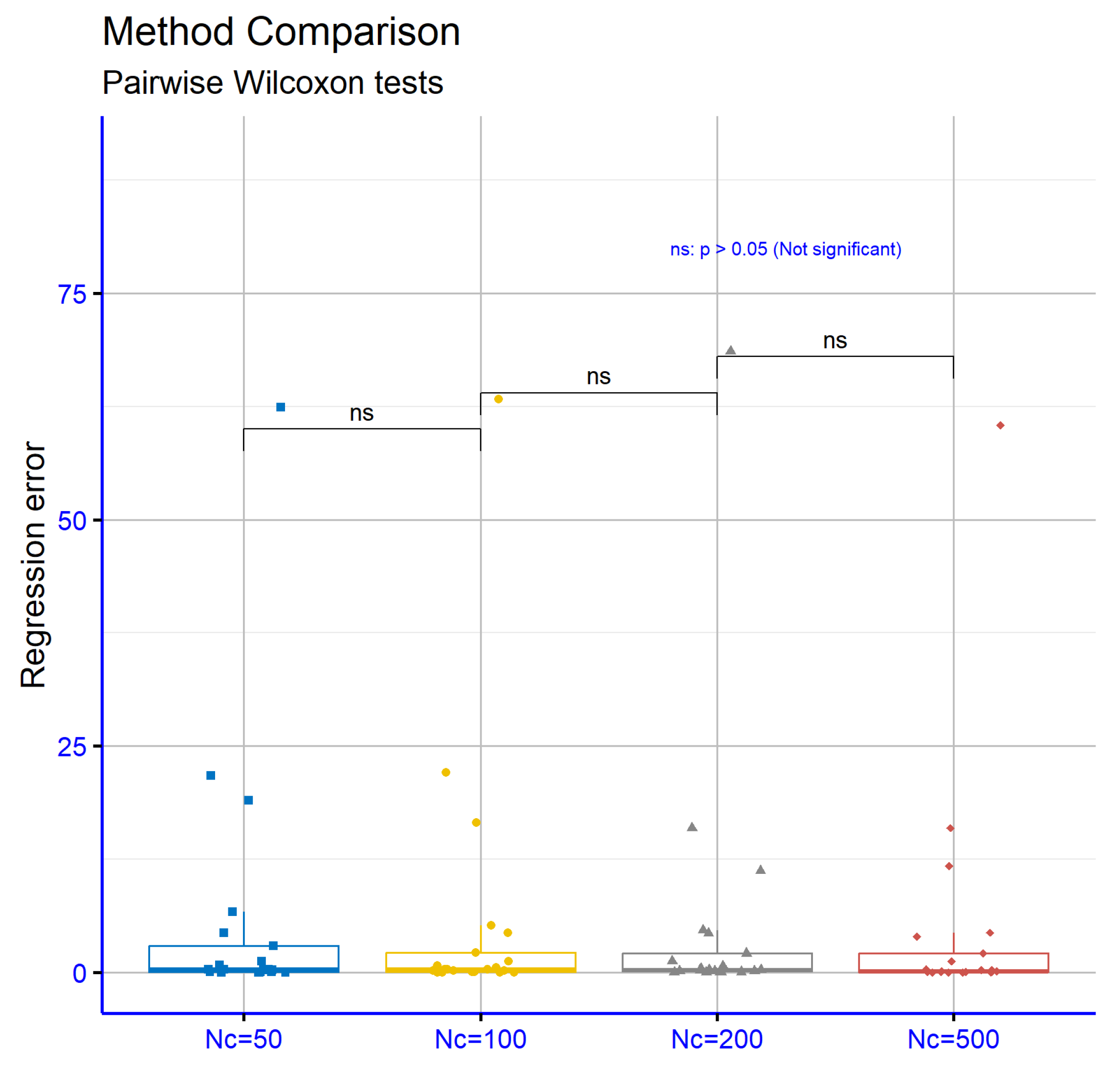
AVERAGE	5.78	5.62	5.28	4.83

presents the absolute prediction errors of the PROPOSED method across the regression datasets, where four different values of $N_c$ were utilized. The general trend observed is a reduction in error as $N_c$ increases, suggesting that greater solution diversity leads to more accurate predictions. This is particularly evident in datasets such as AUTO, BL, HOUSING, STOCK, and TREASURY, where the difference between $N_c=50$ and $N_c=500$ is substantial. In some datasets, such as ABALONE, AIRFOIL, CONCRETE, and LASER, the values remain almost unchanged regardless of $N_c$, indicating that performance in these cases is less dependent on the number of chromosomes. There are also cases with non-monotonic behavior, such as BK and LW, where increasing $N_c$ does not necessarily lead to a consistent reduction in error, possibly due to stochastic factors or overfitting. The mean error steadily decreases from 5.78 for $N_c=50$ to 4.83 for $N_c=500$, reinforcing the overall picture of improvement, although the difference between the two largest $N_c$ values are smaller, which may indicate that the benefit of increasing $N_c$ begins to saturate. Overall, the statistical analysis shows that increasing the number of chromosomes improves the accuracy of the method, with the magnitude of the benefit depending on the specific characteristics of each dataset.

Figure 13 presents the significance levels resulting from the comparisons of classification error rates across datasets for the proposed machine learning method. The comparison between $N_c=50$ and $N_c=100$ shows no significant difference (p = ns), indicating that increasing the number of chromosomes from 50 to 100 does not lead to a substantial improvement. In contrast, the transition from $N_c=100$ to $N_c=200$ shows a statistically significant improvement (p = **), while the increase from $N_c=200$ to $N_c=500$ is also accompanied by a significant difference (p = *), albeit of lower magnitude. These results suggest that higher $N_c$ values can improve performance, with the significance being more pronounced in the mid-range $N_c$ values.

Figure 14 presents the significance levels resulting from the comparisons of prediction errors across regression datasets for the proposed machine learning method. In all three comparisons between $N_c=50$ and $N_c=100$, $N_c=100$ and $N_c=200$, as well as $N_c=200$ and $N_c=500$, the p-value is non-significant (p = ns), indicating that increasing the number of chromosomes does not lead to a statistically significant change in the model’s performance on these datasets.

3.6. Comparison with a Previous Work

Recently, an improved version of the constructed neural networks was published. In this version, the periodical application of a local optimization procedure was suggested [121]. In the following tables, this method is denoted as INNC, and a comparison is made against the original neural network construction procedure (denoted as NNC) and the proposed method (denoted as PROPOSED).

In

Table 8. Experimental results using the constructed neural networks and the two variations for the classification datasets.

DATASET	NNC	INNC	PROPOSED
APPENDICITIS	14.40%	14.70%	16.30%
ALCOHOL	37.72%	29.79%	20.21%
AUSTRALIAN	14.46%	14.80%	14.68%
BALANCE	23.65%	8.66%	7.26%
CLEVELAND	50.93%	47.93%	44.90%
CIRCULAR	12.66%	5.32%	4.22%
DERMATOLOGY	21.54%	20.89%	5.92%
ECOLI	49.88%	48.21%	44.79%
GLASS	56.09%	54.24%	49.43%
HABERMAN	27.53%	26.70%	28.57%
HAYES–ROTH	33.69%	31.77%	30.77%
HEART	15.67%	14.74%	17.85%
HEARTATTACK	20.87%	20.43%	20.67%
HOUSEVOTES	3.17%	3.26%	7.39%
IONOSPHERE	11.29%	11.92%	13.14%
LIVERDISORDER	32.35%	31.77%	33.38%
LYMOGRAPHY	25.29%	25.29%	25.14%
MAMMOGRAPHIC	17.62%	15.81%	17.77%
PARKINSONS	12.74%	12.53%	14.05%
PIMA	28.07%	24.00%	24.34%
POPFAILURES	6.98%	6.44%	7.19%
REGIONS2	26.18%	23.18%	25.00%
SAHEART	29.80%	28.09%	30.11%
SEGMENT	53.50%	43.12%	9.59%
SPIRAL	48.01%	43.99%	41.25%
STATHEART	18.08%	18.67%	20.26%
STUDENT	6.70%	4.55%	7.18%
TRANSFUSION	25.77%	23.43%	23.59%
WDBC	7.36%	4.41%	3.73%
WINE	13.59%	9.77%	10.41%
Z_F_S	14.53%	8.53%	6.60%
Z_O_N_F_S	48.62%	38.58%	49.66%
ZO_NF_S	13.54%	6.84%	3.94%
ZONF_S	2.64%	2.52%	2.60%
ZOO	8.70%	7.20%	5.10%
AVERAGE	23.82%	20.92%	19.63%

, the comparison of mean error rates shows that the PROPOSED method achieves the lowest average error rate, 19.63%, compared to 20.92% for INNC and 23.82% for NNC, indicating an overall improvement in performance. In several datasets, such as ALCOHOL, BALANCE, CIRCULAR, DERMATOLOGY, GLASS, SEGMENT, and ZO_NF_S, the PROPOSED method clearly outperforms the others, recording substantially lower error rates than the two comparative models. However, in certain cases, such as HABERMAN, HEART, HOUSEVOTES, and IONOSPHERE, the proposed method shows slightly higher error than the best-performing of the other two models, suggesting that its superiority is not universal. There are also instances of equivalent or marginal differences, such as in LYMOGRAPHY and ZONF_S, where the performances of all three methods are very close. The overall trend indicates that the proposed method often achieves a significant reduction in error, with improvements being more pronounced in datasets with higher complexity or diversity in classes.

In

Table 9. Experimental results using the constructed neural networks and the two variations on the regression datasets.

DATASET	NNC	INNC	PROPOSED
ABALONE	5.08	4.33	4.41
AIRFOIL	0.004	0.002	0.001
AUTO	17.13	11.01	11.73
BK	0.10	0.07	0.058
BL	1.19	0.002	0.13
BASEBALL	61.57	48.42	60.42
CONCRETE	0.008	0.005	0.004
DEE	0.26	0.23	0.26
FRIEDMAN	6.29	4.88	1.25
FY	0.11	0.042	0.13
HO	0.015	0.01	0.073
HOUSING	25.47	16.01	15.96
LASER	0.025	0.006	0.004
LW	0.011	0.012	0.32
MORTGAGE	0.30	0.026	0.15
PL	0.047	0.022	0.021
PLASTIC	4.20	2.25	2.15
QUAKE	0.96	0.04	0.061
SN	0.026	0.026	0.10
STOCK	8.92	6.33	3.96
TREASURY	0.43	0.066	0.25
AVERAGE	6.29	4.47	4.83

, the comparison of mean errors shows that INNC has the lowest average value (4.47), followed by the PROPOSED method (4.83) and NNC (6.29), indicating that the proposed method demonstrates an overall improvement over NNC but falls slightly short of INNC. In several datasets, such as AIRFOIL, CONCRETE, LASER, PL, PLASTIC, and STOCK, the PROPOSED method achieves the lowest or highly competitive error values, showing clear improvement over NNC and, in some cases, over INNC as well. However, in certain cases, such as AUTO, BASEBALL, FRIEDMAN, LW, and SN, INNC outperforms with lower errors, while there are also instances where NNC achieves better performance than the PROPOSED method, such as in DEE and FY, although the differences are small. The overall picture indicates that the PROPOSED method can achieve significant improvement in specific regression problems, but its superiority is not universal, with its performance depending on the characteristics of each dataset.

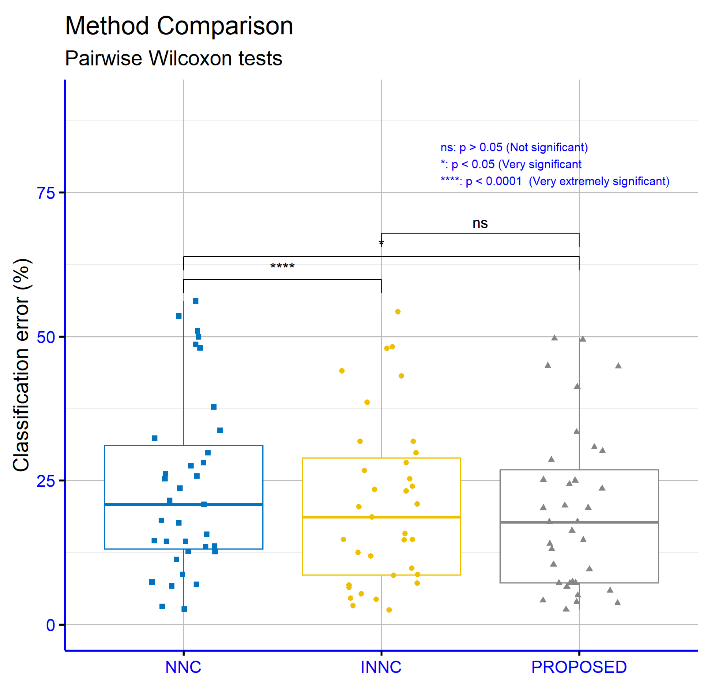
Figure 15 presents the significance levels resulting from the comparisons of error rates on classification datasets for the proposed machine learning method in relation to the NNC and INNC models. The comparison between NNC and INNC shows extremely high statistical significance (p = ****), indicating a clear superiority of INNC. The comparison between NNC and the PROPOSED method also shows a statistically significant difference (p = *), indicating that the PROPOSED method outperforms NNC. In contrast, the comparison between INNC and the PROPOSED method does not show a statistically significant difference, suggesting that the two methods perform similarly on these datasets.

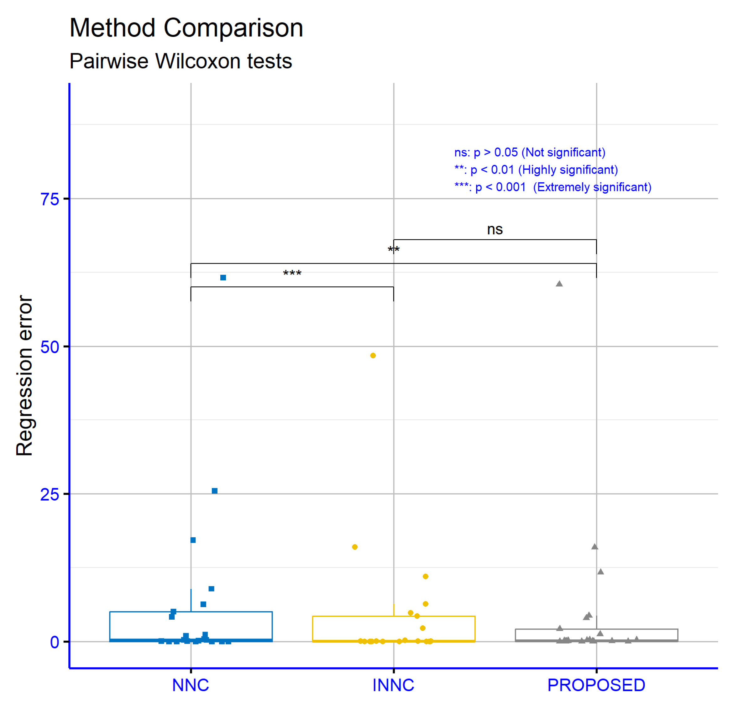
Figure 16 presents the significance levels from the comparisons of error rates on classification datasets for the proposed machine learning method in relation to the NNC and INNC models. The comparison between NNC and INNC shows high statistical significance (p = ***), indicating a clear superiority of INNC. The comparison between NNC and the PROPOSED method also shows a statistically significant difference (p = **), demonstrating the improvement of the PROPOSED method over NNC. In contrast, the comparison between INNC and the PROPOSED method does not show a statistically significant difference, indicating that the two methods have comparable performance on these datasets.

Also, it should be noted that the INNC method requires significantly more time than the PROPOSED method, since it applies several applications of the local search procedure on randomly selected chromosomes.

4. Conclusions

This study clearly demonstrates the importance of integrating a preliminary training phase into the grammar-based evolution framework for constructing artificial neural networks. The role of this pretraining phase extends far beyond merely initializing the solution space. It effectively enhances the quality of the initial population by transferring information from a previously trained neural network, resulting in a better-informed starting point for the evolutionary process. This enriched initialization improves convergence rates and reduces the risk of stagnation in local minima, especially in complex, non-linear, or noisy problem domains.

Experimental findings show that the proposed approach not only achieves improved numerical performance metrics, but also exhibits increased consistency across diverse datasets. Unlike many conventional methods that are often sensitive to the nature of the data and prone to high variability in performance, the proposed model demonstrates both robustness and generalization capability. This makes it a strong candidate for applications in high-stakes or real-time environments where model reliability is critical, such as in medical diagnosis, energy forecasting, or financial decision-making.

The sensitivity analysis concerning the initialization factor ($I_w$) offers further insight into the behavior of the proposed model. Although the differences among parameter values are not statistically significant, a consistent trend toward improved accuracy with higher Iw values suggests that careful tuning of initialization can have a meaningful impact on model effectiveness. In more complex datasets, higher $I_w$ settings appear to support better generalization, pointing to the potential of initialization strategies as a lever for optimization.

Overall, the proposed system should not be viewed as a minor variation on existing grammar evolution techniques, but rather as a substantial advancement in how prior knowledge and pretraining experience can be exploited to improve and accelerate evolutionary learning. This approach merges the advantages of pretraining with the adaptability of evolutionary search, forming a solid foundation for future developments involving hybrid or meta-intelligent strategies in automated neural architecture design. Its demonstrated performance, adaptability, and potential for integration with broader machine learning paradigms mark it as a promising direction for ongoing and future exploration.

Regarding future research directions, there are several promising avenues to explore. One potential extension of the current study could involve the use of alternative pretraining techniques beyond genetic algorithms, such as particle swarm optimization or differential evolution, to assess the influence of various optimization strategies on the initial population. Additionally, it would be valuable to examine the role of the pretraining phase in relation to variables such as the number of nodes, the level of noise in the data, and feature heterogeneity.

At this stage, the proposed work is applied to single-hidden layer artificial neural networks. However, with appropriate modification of the BNF grammar that generates the above networks, it could also be applied to deep learning models, although this would require significantly more computational resources, thus making the use of parallel processing techniques a necessity.

Finally, it is suggested that reinforcement learning techniques or even hybrid models such as GANs and Autoencoders be incorporated into the grammar-based evolution framework. Combining the proposed pretraining phase with neural architecture search methodologies could lead to even more efficient and generalizable models. The demonstrated stability and adaptability of the proposed approach make it a strong candidate for application in demanding real-world domains such as healthcare, energy, and financial forecasting.

References

1. Abiodun, O.I.; Jantan, A.; Omolara, A.E.; Dada, K.V.; Mohamed, N.A.; Arshad, H. State-of-the-art in artificial neural network applications: A survey. Heliyon 2018, 4, e00938. [Google Scholar] [CrossRef]
2. Suryadevara, S.; Yanamala, A.K.Y. A Comprehensive Overview of Artificial Neural Networks: Evolution, Architectures, and Applications. Rev. Intel. Artif. Med. 2021, 12, 51–76. [Google Scholar]
3. Egmont-Petersen, M.; de Ridder, D.; Handels, H. Image processing with neural networks—A review. Pattern Recognit. 2002, 35, 2279–2301. [Google Scholar] [CrossRef]
4. Zhang, G.P. Time series forecasting using a hybrid ARIMA and neural network model. Neurocomputing 2003, 50, 159–175. [Google Scholar] [CrossRef]
5. Huang, Z.; Chen, H.; Hsu, C.-J.; Chen, W.-H.; Wu, S. Credit rating analysis with support vector machines and neural networks: A market comparative study. Decis. Support Syst. 2004, 37, 543–558. [Google Scholar] [CrossRef]
6. Baldi, P.; Cranmer, K.; Faucett, T.; Sadowski, P.; Whiteson, D. Parameterized neural networks for high-energy physics. Eur. Phys. J. C 2016, 76, 1–7. [Google Scholar] [CrossRef]
7. Kia, M.B.; Pirasteh, S.; Pradhan, B.; Mahmud, A.R.; Sulaiman, W.N.; Moradi, A. An artificial neural network model for flood simulation using GIS: Johor River Basin, Malaysia. Environ. Earth Sci. 2012, 67, 251–264. [Google Scholar] [CrossRef]
8. Yadav, A.K.; Chandel, S.S. Solar radiation prediction using Artificial Neural Network techniques: A review. Renew. Sustain. Energy Rev. 2014, 33, 772–781. [Google Scholar] [CrossRef]
9. Getahun, M.A.; Shitote, S.M.; Zachary, C. Artificial neural network based modelling approach for strength prediction of concrete incorporating agricultural and construction wastes. Constr. Build. Mater. 2018, 190, 517–525. [Google Scholar] [CrossRef]
10. Chen, M.; Challita, U.; Saad, W.; Yin, C.; Debbah, M. Artificial Neural Networks-Based Machine Learning for Wireless Networks: A Tutorial. IEEE Commun. Surv. Tutor. 2019, 21, 3039–3071. [Google Scholar] [CrossRef]
11. Peta, K.; Żurek, J. Prediction of air leakage in heat exchangers for automotive applications using artificial neural networks. In Proceedings of the 2018 9th IEEE Annual Ubiquitous Computing, Electronics & Mobile Communication Conference (UEMCON), New York, NY, USA, 8–10 November 2018; pp. 721–725. [Google Scholar]
12. Vora, K.; Yagnik, S. A survey on backpropagation algorithms for feedforward neural networks. Int. J. Eng. Dev. Res. 2014, 1, 193–197. [Google Scholar]
13. Pajchrowski, T.; Zawirski, K.; Nowopolski, K. Neural speed controller trained online by means of modified RPROP algorithm. IEEE Trans. Ind. Inform. 2014, 11, 560–568. [Google Scholar] [CrossRef]
14. Hermanto, R.P.S.; Nugroho, A. Waiting-time estimation in bank customer queues using RPROP neural networks. Procedia Comput. Sci. 2018, 135, 35–42. [Google Scholar] [CrossRef]
15. Reynolds, J.; Rezgui, Y.; Kwan, A.; Piriou, S. A zone-level, building energy optimisation combining an artificial neural network, a genetic algorithm, and model predictive control. Energy 2018, 151, 729–739. [Google Scholar] [CrossRef]
16. Das, G.; Pattnaik, P.K.; Padhy, S.K. Artificial neural network trained by particle swarm optimization for non-linear channel equalization. Expert Syst. Appl. 2014, 41, 3491–3496. [Google Scholar] [CrossRef]
17. Sexton, R.S.; Dorsey, R.E.; Johnson, J.D. Beyond backpropagation: Using simulated annealing for training neural networks. J. Organ. End User Comput. (JOEUC) 1999, 11, 3–10. [Google Scholar] [CrossRef]
18. Wang, L.; Zeng, Y.; Chen, T. Back propagation neural network with adaptive differential evolution algorithm for time series forecasting. Expert Syst. Appl. 2015, 42, 855–863. [Google Scholar] [CrossRef]
19. Karaboga, D.; Akay, B. Artificial bee colony (ABC) algorithm on training artificial neural networks. In Proceedings of the 2007 IEEE 15th Signal Processing and Communications Applications, Eskisehir, Turkey, 11–13 June 2007; pp. 1–4. [Google Scholar]
20. Sexton, R.S.; Alidaee, B.; Dorsey, R.E.; Johnson, J.D. Global optimization for artificial neural networks: A tabu search application. Eur. J. Oper. Res. 1998, 106, 570–584. [Google Scholar] [CrossRef]
21. Zhang, J.-R.; Zhang, J.; Lok, T.-M.; Lyu, M.R. A hybrid particle swarm optimization–back-propagation algorithm for feedforward neural network training. Appl. Math. Comput. 2007, 185, 1026–1037. [Google Scholar] [CrossRef]
22. Zhao, G.; Wang, T.; Jin, Y.; Lang, C.; Li, Y.; Ling, H. The Cascaded Forward algorithm for neural network training. Pattern Recognit. 2025, 161, 111292. [Google Scholar] [CrossRef]
23. Oh, K.-S.; Jung, K. GPU implementation of neural networks. Pattern Recognit. 2004, 37, 1311–1314. [Google Scholar] [CrossRef]
24. Zhang, M.; Hibi, K.; Inoue, J. GPU-accelerated artificial neural network potential for molecular dynamics simulation. Comput. Commun. 2023, 285, 108655. [Google Scholar] [CrossRef]
25. Nowlan, S.J.; Hinton, G.E. Simplifying neural networks by soft weight sharing. Neural Comput. 1992, 4, 473–493. [Google Scholar] [CrossRef]
26. Hanson, S.J.; Pratt, L.Y. Comparing biases for minimal network construction with back propagation. In Advances in Neural Information Processing Systems; Touretzky, D.S., Ed.; Morgan Kaufmann: San Mateo, CA, USA, 1989; Volume 1, pp. 177–185. [Google Scholar]
27. Augasta, M.; Kathirvalavakumar, T. Pruning algorithms of neural networks—A comparative study. Cent. Eur. Comput. Sci. 2003, 3, 105–115. [Google Scholar] [CrossRef]
28. Prechelt, L. Automatic early stopping using cross validation: Quantifying the criteria. Neural Netw. 1998, 11, 761–767. [Google Scholar] [CrossRef] [PubMed]
29. Wu, X.; Liu, J. A New Early Stopping Algorithm for Improving Neural Network Generalization. In Proceedings of the 2009 Second International Conference on Intelligent Computation Technology and Automation, Changsha, China, 10–11 October 2009; pp. 15–18. [Google Scholar]
30. Treadgold, N.K.; Gedeon, T.D. Simulated annealing and weight decay in adaptive learning: The SARPROP algorithm. IEEE Trans. Neural Netw. 1998, 9, 662–668. [Google Scholar] [CrossRef] [PubMed]
31. Carvalho, M.; Ludermir, T.B. Particle Swarm Optimization of Feed-Forward Neural Networks with Weight Decay. In Proceedings of the 2006 Sixth International Conference on Hybrid Intelligent Systems (HIS’06), Rio de Janeiro, Brazil, 13–15 December 2006; p. 5. [Google Scholar]
32. Arifovic, J.; Gençay, R. Using genetic algorithms to select architecture of a feedforward artificial neural network. Phys. A Stat. Mech. Its Appl. 2001, 289, 574–594. [Google Scholar] [CrossRef]
33. Benardos, P.G.; Vosniakos, G.C. Optimizing feedforward artificial neural network architecture. Eng. Appl. Artif. Intell. 2007, 20, 365–382. [Google Scholar] [CrossRef]
34. Garro, B.A.; Vázquez, R.A. Designing Artificial Neural Networks Using Particle Swarm Optimization Algorithms. Comput. Neurosci. 2015, 2015, 369298. [Google Scholar] [CrossRef]
35. Siebel, N.T.; Sommer, G. Evolutionary reinforcement learning of artificial neural networks. Int. Hybrid Intell. Syst. 2007, 4, 171–183. [Google Scholar]
36. Jaafra, Y.; Laurent, J.L.; Deruyver, A.; Naceur, M.S. Reinforcement learning for neural architecture search: A review. Image Vis. Comput. 2019, 89, 57–66. [Google Scholar] [CrossRef]
37. Pham, H.; Guan, M.; Zoph, B.; Le, Q.; Dean, J. Efficient neural architecture search via parameters sharing. In Proceedings of the 35th International Conference on Machine Learning, PMLR, Stockholm, Sweden, 10–15 July 2018; pp. 4095–4104. [Google Scholar]
38. Xie, S.; Zheng, H.; Liu, C.; Lin, L. SNAS: Stochastic neural architecture search. arXiv 2018, arXiv:1812.09926. [Google Scholar]
39. Zhou, H.; Yang, M.; Wang, J.; Pan, W. Bayesnas: A bayesian approach for neural architecture search. In Proceedings of the 36th International Conference on Machine Learning, PMLR, Long Beach, CA, USA, 10–15 June 2019; pp. 7603–7613. [Google Scholar]
40. O’Neill, M.; Ryan, C. Grammatical evolution. IEEE Trans. Evol. Comput. 2001, 5, 349–358. [Google Scholar] [CrossRef]
41. Tsoulos, I.G.; Gavrilis, D.; Glavas, E. Neural network construction and training using grammatical evolution. Neurocomputing 2008, 72, 269–277. [Google Scholar] [CrossRef]
42. Papamokos, G.V.; Tsoulos, I.G.; Demetropoulos, I.N.; Glavas, E. Location of amide I mode of vibration in computed data utilizing constructed neural networks. Expert Syst. Appl. 2009, 36, 12210–12213. [Google Scholar] [CrossRef]
43. Tsoulos, I.G.; Gavrilis, D.; Glavas, E. Solving differential equations with constructed neural networks. Neurocomputing 2009, 72, 2385–2391. [Google Scholar] [CrossRef]
44. Tsoulos, I.G.; Mitsi, G.; Stavrakoudis, A.; Papapetropoulos, S. Application of Machine Learning in a Parkinson’s Disease Digital Biomarker Dataset Using Neural Network Construction (NNC) Methodology Discriminates Patient Motor Status. Front. ICT 2019, 6, 10. [Google Scholar] [CrossRef]
45. Christou, V.; Tsoulos, I.G.; Loupas, V.; Tzallas, A.T.; Gogos, C.; Karvelis, P.S.; Antoniadis, N.; Glavas, E.; Giannakeas, N. Performance and early drop prediction for higher education students using machine learning. Expert Syst. Appl. 2023, 225, 120079. [Google Scholar] [CrossRef]
46. Toki, E.I.; Pange, J.; Tatsis, G.; Plachouras, K.; Tsoulos, I.G. Utilizing Constructed Neural Networks for Autism Screening. Appl. Sci. 2024, 14, 3053. [Google Scholar] [CrossRef]
47. Li, G.; Alnuweiri, H.; Wu, Y.; Li, H. Acceleration of back propagation through initial weight pre-training with delta rule. In Proceedings of the IEEE International Conference on neural networks, San Francisco, CA, USA, 28 March–1 April 1993; pp. 580–585. [Google Scholar]
48. Erhan, D.; Courville, A.; Bengio, Y.; Vincent, P. Why does unsupervised pre-training help deep learning? In Proceedings of the Thirteenth International Conference on Artificial Intelligence and Statistics, JMLR Workshop and Conference Proceedings, Sardinia, Italy, 13–15 May 2010; pp. 201–208. [Google Scholar]
49. Owhadi-Kareshk, M.; Sedaghat, Y.; Akbarzadeh-T, M.R. Pre-training of an artificial neural network for software fault prediction. In Proceedings of the 2017 IEEE 7th International Conference on Computer and Knowledge Engineering (ICCKE), Mashhad, Iran, 26–27 October 2017; pp. 223–228. [Google Scholar]
50. Saikia, P.; Vij, P.; Baruah, R.D. Unsupervised pre-training on improving the performance of neural network in regression. In Proceedings of the IEEE 2018 International Joint Conference on Neural Networks (IJCNN), Rio de Janeiro, Brazil, 8–13 July 2018; pp. 1–6. [Google Scholar]
51. Kroshchanka, A.; Golovko, V. The reduction of fully connected neural network parameters using the pre-training technique. In Proceedings of the 2021 11th IEEE International Conference on Intelligent Data Acquisition and Advanced Computing Systems: Technology and Applications (IDAACS), Cracow, Poland, 22–25 September 2021; Volume 2, pp. 937–941. [Google Scholar]
52. Noinongyao, P.; Watchareeruetai, U. An extreme learning machine based pretraining method for multi-layer neural networks. In Proceedings of the 2018 Joint 10th International Conference on Soft Computing and Intelligent Systems (SCIS) and 19th International Symposium on Advanced Intelligent Systems (ISIS), Toyama, Japan, 5–8 December 2018; pp. 608–613. [Google Scholar]
53. Holland, J.H. Genetic algorithms. Sci. Am. 1992, 267, 66–73. [Google Scholar] [CrossRef]
54. Stender, J. Parallel Genetic Algorithms: Theory & Applications; IOS Press: Amsterdam, The Netherlands, 1993. [Google Scholar]
55. Goldberg, D. Genetic Algorithms in Search, Optimization and Machine Learning; Addison-Wesley Publishing Company: Reading, MA, USA, 1989. [Google Scholar]
56. Michaelewicz, Z. Genetic Algorithms + Data Structures = Evolution Programs; Springer: Berlin/Heidelberg, Germany, 1996. [Google Scholar]
57. Liu, X.; Jiang, D.; Tao, B.; Jiang, G.; Sun, Y.; Kong, J.; Chen, B. Genetic algorithm-based trajectory optimization for digital twin robots. Front. Bioeng. Biotechnol. 2022, 9, 793782. [Google Scholar] [CrossRef] [PubMed]
58. Min, D.; Song, Z.; Chen, H.; Wang, T.; Zhang, T. Genetic algorithm optimized neural network based fuel cell hybrid electric vehicle energy management strategy under start-stop condition. Appl. Energy 2022, 306, 118036. [Google Scholar] [CrossRef]
59. Chen, Q.; Hu, X. Design of intelligent control system for agricultural greenhouses based on adaptive improved genetic algorithm for multi-energy supply system. Energy Rep. 2022, 8, 12126–12138. [Google Scholar] [CrossRef]
60. Hornik, K.; Stinchcombe, M.; White, H. Multilayer feedforward networks are universal approximators. Neural Netw. 1989, 2, 359–366. [Google Scholar] [CrossRef]
61. Kaelo, P.; Ali, M.M. Integrated crossover rules in real coded genetic algorithms. Eur. J. Oper. Res. 2007, 176, 60–76. [Google Scholar] [CrossRef]
62. Backus, J.W. The Syntax and Semantics of the Proposed International Algebraic Language of the Zurich ACM-GAMM Conference. In Proceedings of the International Conference on Information Processing, UNESCO, Paris, France, 15–20 June 1959; pp. 125–132. [Google Scholar]
63. Ryan, C.; Collins, J.; O’Neill, M. Grammatical evolution: Evolving programs for an arbitrary language. In Genetic Programming. EuroGP 1998; Banzhaf, W., Poli, R., Schoenauer, M., Fogarty, T.C., Eds.; Lecture Notes in Computer Science; Springer: Berlin/Heidelberg, Germany, 1998; Volume 1391. [Google Scholar]
64. O’Neill, M.; Ryan, M.C. Evolving Multi-line Compilable C Programs. In Genetic Programming. EuroGP 1999; Poli, R., Nordin, P., Langdon, W.B., Fogarty, T.C., Eds.; Lecture Notes in Computer Science; Springer: Berlin/Heidelberg, Germany, 1999; Volume 1598. [Google Scholar]
65. Puente, A.O.; Alfonso, R.S.; Moreno, M.A. Automatic composition of music by means of grammatical evolution. In Proceedings of the 2002 Conference on APL: Array Processing Languages: Lore, Problems, and Applications, APL’02, Madrid, Spain, 22–25 July 2002; pp. 148–155. [Google Scholar]
66. Galván-López, E.; Swafford, J.M.; O’Neill, M.; Brabazon, A. Evolving a Ms. PacMan Controller Using Grammatical Evolution. In Applications of Evolutionary Computation; EvoApplications 2010. Lecture Notes in Computer Science; Springer: Berlin/Heidelberg, Germany, 2010; Volume 6024. [Google Scholar]
67. Shaker, N.; Nicolau, M.; Yannakakis, G.N.; Togelius, J.; O’Neill, M. Evolving levels for Super Mario Bros using grammatical evolution. In Proceedings of the 2012 IEEE Conference on Computational Intelligence and Games (CIG), Granada, Spain, 11–14 September 2012; pp. 304–331. [Google Scholar]
68. Martínez-Rodríguez, D.; Colmenar, J.M.; Hidalgo, J.I.; Micó, R.J.V.; Salcedo-Sanz, S. Particle swarm grammatical evolution for energy demand estimation. Energy Sci. Eng. 2020, 8, 1068–1079. [Google Scholar] [CrossRef]
69. Ryan, C.; Kshirsagar, M.; Vaidya, G.; Cunningham, A.; Sivaraman, R. Design of a cryptographically secure pseudo random number generator with grammatical evolution. Sci. Rep. 2022, 12, 8602. [Google Scholar] [CrossRef]
70. Martín, C.; Quintana, D.; Isasi, P. Grammatical Evolution-based ensembles for algorithmic trading. Appl. Soft Comput. 2019, 84, 105713. [Google Scholar] [CrossRef]
71. Kelly, M.; Longjohn, R.; Nottingham, K. The UCI Machine Learning Repository. Available online: https://archive.ics.uci.edu (accessed on 11 September 2025).
72. Alcalá-Fdez, J.; Fernandez, A.; Luengo, J.; Derrac, J.; García, S.; Sánchez, L.; Herrera, F. KEEL Data-Mining Software Tool: Data Set Repository, Integration of Algorithms and Experimental Analysis Framework. J. Mult.-Valued Log. Soft Comput. 2011, 17, 255–287. [Google Scholar]
73. Weiss, S.M.; Kulikowski, C.A. Computer Systems That Learn: Classification and Prediction Methods from Statistics, Neural Nets, Machine Learning, and Expert Systems; Morgan Kaufmann Publishers Inc.: San Francisco, CA, USA, 1991. [Google Scholar]
74. Tzimourta, K.D.; Tsoulos, I.; Bilero, I.T.; Tzallas, A.T.; Tsipouras, M.G.; Giannakeas, N. Direct Assessment of Alcohol Consumption in Mental State Using Brain Computer Interfaces and Grammatical Evolution. Inventions 2018, 3, 51. [Google Scholar] [CrossRef]
75. Quinlan, J.R. Simplifying Decision Trees. Int. J. Man-Mach. Stud. 1987, 27, 221–234. [Google Scholar] [CrossRef]
76. Shultz, T.; Mareschal, D.; Schmidt, W. Modeling Cognitive Development on Balance Scale Phenomena. Mach. Learn. 1994, 16, 59–88. [Google Scholar] [CrossRef]
77. Zhou, Z.H.; Jiang, Y. NeC4.5: Neural ensemble based C4.5. IEEE Trans. Knowl. Data Eng. 2004, 16, 770–773. [Google Scholar] [CrossRef]
78. Setiono, R.; Leow, W.K. FERNN: An Algorithm for Fast Extraction of Rules from Neural Networks. Appl. Intell. 2000, 12, 15–25. [Google Scholar] [CrossRef]
79. Demiroz, G.; Govenir, H.A.; Ilter, N. Learning Differential Diagnosis of Eryhemato-Squamous Diseases using Voting Feature Intervals. Artif. Intell. Med. 1998, 13, 147–165. [Google Scholar]
80. Horton, P.; Nakai, K. A Probabilistic Classification System for Predicting the Cellular Localization Sites of Proteins. In Proceedings of the International Conference on Intelligent Systems for Molecular Biology, St. Louis, MO, USA, 12–15 June 1996; Volume 4, pp. 109–115. [Google Scholar]
81. Hayes-Roth, B.; Hayes-Roth, B.F. Concept learning and the recognition and classification of exemplars. J. Verbal Learn. Verbal Behav. 1977, 16, 321–338. [Google Scholar] [CrossRef]
82. Kononenko, I.; Šimec, E.; Robnik-Šikonja, M. Overcoming the Myopia of Inductive Learning Algorithms with RELIEFF. Appl. Intell. 1997, 7, 39–55. [Google Scholar] [CrossRef]
83. French, R.M.; Chater, N. Using noise to compute error surfaces in connectionist networks: A novel means of reducing catastrophic forgetting. Neural Comput. 2002, 14, 1755–1769. [Google Scholar] [CrossRef]
84. Dy, J.G.; Brodley, C.E. Feature Selection for Unsupervised Learning. J. Mach. Learn. Res. 2004, 5, 845–889. [Google Scholar]
85. Perantonis, S.J.; Virvilis, V. Input Feature Extraction for Multilayered Perceptrons Using Supervised Principal Component Analysis. Neural Process. Lett. 1999, 10, 243–252. [Google Scholar] [CrossRef]
86. Garcke, J.; Griebel, M. Classification with sparse grids using simplicial basis functions. Intell. Data Anal. 2002, 6, 483–502. [Google Scholar] [CrossRef]
87. Mcdermott, J.; Forsyth, R.S. Diagnosing a disorder in a classification benchmark. Pattern Recognit. Lett. 2016, 73, 41–43. [Google Scholar] [CrossRef]
88. Cestnik, G.; Konenenko, I.; Bratko, I. Assistant-86: A Knowledge-Elicitation Tool for Sophisticated Users. In Progress in Machine Learning; Bratko, I., Lavrac, N., Eds.; Sigma Press: Wilmslow, UK, 1987; pp. 31–45. [Google Scholar]
89. Elter, M.; Schulz-Wendtland, R.; Wittenberg, T. The prediction of breast cancer biopsy outcomes using two CAD approaches that both emphasize an intelligible decision process. Med. Phys. 2007, 34, 4164–4172. [Google Scholar]
90. Little, M.A.; McSharry, P.E.; Roberts, S.J.; Costello, D.; Moroz, I. Exploiting Nonlinear Recurrence and Fractal Scaling Properties for Voice Disorder Detection. Nat. Preced. 2007, 6, 23. [Google Scholar]
91. Little, M.A.; McSharry, P.E.; Hunter, E.J.; Spielman, J.; Ramig, L.O. Suitability of dysphonia measurements for telemonitoring of Parkinson’s disease. IEEE Trans. Biomed. Eng. 2009, 56, 1015–1022. [Google Scholar]
92. Smith, J.W.; Everhart, J.E.; Dickson, W.C.; Knowler, W.C.; Johannes, R.S. Using the ADAP learning algorithm to forecast the onset of diabetes mellitus. In Proceedings of the Symposium on Computer Applications and Medical Care, Washington, DC, USA, 6–9 November 1988; IEEE Computer Society Press: Los Alamitos, CA, USA, 1988; pp. 261–265. [Google Scholar]
93. Lucas, D.D.; Klein, R.; Tannahill, J.; Ivanova, D.; Brandon, S.; Domyancic, D.; Zhang, Y. Failure analysis of parameter-induced simulation crashes in climate models. Geosci. Dev. 2013, 6, 1157–1171. [Google Scholar] [CrossRef]
94. Giannakeas, N.; Tsipouras, M.G.; Tzallas, A.T.; Kyriakidi, K.; Tsianou, Z.E.; Manousou, P.; Hall, A.; Karvounis, E.C.; Tsianos, V.; Tsianos, E. A clustering based method for collagen proportional area extraction in liver biopsy images. In Proceedings of the Annual International Conference of the IEEE Engineering in Medicine and Biology Society, EMBS, Milan, Italy, 25–29 August 2015; pp. 3097–3100. [Google Scholar]
95. Hastie, T.; Tibshirani, R. Non-parametric logistic and proportional odds regression. JRSS-C (Appl. Stat.) 1987, 36, 260–276. [Google Scholar] [CrossRef]
96. Dash, M.; Liu, H.; Scheuermann, P.; Tan, K.L. Fast hierarchical clustering and its validation. Data Knowl. Eng. 2003, 44, 109–138. [Google Scholar] [CrossRef]
97. Cortez, P.; Silva, A.M.G. Using data mining to predict secondary school student performance. In Proceedings of the 5th FUture BUsiness TEChnology Conference (FUBUTEC 2008), EUROSIS-ETI, Porto, Portugal, 9–11 April 2008; pp. 5–12. [Google Scholar]
98. Yeh, I.-C.; Yang, K.-J.; Ting, T.-M. Knowledge discovery on RFM model using Bernoulli sequence. Expert. Appl. 2009, 36, 5866–5871. [Google Scholar]
99. Jeyasingh, S.; Veluchamy, M. Modified bat algorithm for feature selection with the Wisconsin diagnosis breast cancer (WDBC) dataset. Asian Pac. J. Cancer Prev. APJCP 2017, 18, 1257. [Google Scholar]
100. Alshayeji, M.H.; Ellethy, H.; Gupta, R. Computer-aided detection of breast cancer on the Wisconsin dataset: An artificial neural networks approach. Biomed. Signal Process. Control 2022, 71, 103141. [Google Scholar] [CrossRef]
101. Raymer, M.; Doom, T.E.; Kuhn, L.A.; Punch, W.F. Knowledge discovery in medical and biological datasets using a hybrid Bayes classifier/evolutionary algorithm. IEEE Trans. Syst. Man Cybern. Part B (Cybern.) 2003, 33, 802–813. [Google Scholar] [CrossRef] [PubMed]
102. Zhong, P.; Fukushima, M. Regularized nonsmooth Newton method for multi-class support vector machines. Optim. Methods Softw. 2007, 22, 225–236. [Google Scholar] [CrossRef]
103. Andrzejak, R.G.; Lehnertz, K.; Mormann, F.; Rieke, C.; David, P.; Elger, C.E. Indications of nonlinear deterministic and finite-dimensional structures in time series of brain electrical activity: Dependence on recording region and brain state. Phys. Rev. E 2001, 64, 061907. [Google Scholar] [CrossRef]
104. Tzallas, A.T.; Tsipouras, M.G.; Fotiadis, D.I. Automatic Seizure Detection Based on Time-Frequency Analysis and Artificial Neural Networks. Comput. Intell. Neurosci. 2007, 2007, 80510. [Google Scholar] [CrossRef]
105. Koivisto, M.; Sood, K. Exact Bayesian Structure Discovery in Bayesian Networks. J. Mach. Learn. Res. 2004, 5, 549–573. [Google Scholar]
106. Nash, W.J.; Sellers, T.L.; Talbot, S.R.; Cawthor, A.J.; Ford, W.B. The Population Biology of Abalone (Haliotis species) in Tasmania. I. Blacklip Abalone (H. rubra) from the North Coast and Islands of Bass Strait, Sea Fisheries Division; Technical Report No. 48; Department of Primary Industry and Fisheries, Tasmania: Hobart, Australia, 1994; ISSN 1034-3288. [Google Scholar]
107. Brooks, T.F.; Pope, D.S.; Marcolini, A.M. Airfoil Self-Noise and Prediction. Technical Report, NASA RP-1218. July 1989. Available online: https://ntrs.nasa.gov/citations/19890016302 (accessed on 14 November 2024).
108. Yeh, I.C. Modeling of strength of high performance concrete using artificial neural networks. Cem. Concrete Res. 1998, 28, 1797–1808. [Google Scholar] [CrossRef]
109. Friedman, J. Multivariate Adaptative Regression Splines. Ann. Stat. 1991, 19, 1–141. [Google Scholar]
110. Harrison, D.; Rubinfeld, D.L. Hedonic housing prices and the demand for clean air. J. Environ. Econ. Manag. 1978, 5, 81–102. [Google Scholar] [CrossRef]
111. Tsoulos, I.G.; Charilogis, V.; Kyrou, G.; Stavrou, V.N.; Tzallas, A. OPTIMUS: A Multidimensional Global Optimization Package. J. Open Source Softw. 2025, 10, 7584. [Google Scholar] [CrossRef]
112. Kingma, D.P.; Ba, J.L. ADAM: A method for stochastic optimization. In Proceedings of the 3rd International Conference on Learning Representations (ICLR 2015), San Diego, CA, USA, 7–9 May 2015; pp. 1–15. [Google Scholar]
113. Powell, M.J.D. A Tolerant Algorithm for Linearly Constrained Optimization Calculations. Math. Program. 1989, 45, 547–566. [Google Scholar] [CrossRef]
114. Park, J.; Sandberg, I.W. Universal Approximation Using Radial-Basis-Function Networks. Neural Comput. 1991, 3, 246–257. [Google Scholar] [CrossRef] [PubMed]
115. Montazer, G.A.; Giveki, D.; Karami, M.; Rastegar, H. Radial basis function neural networks: A review. Comput. Rev. J. 2018, 1, 52–74. [Google Scholar]
116. Stanley, K.O.; Miikkulainen, R. Evolving Neural Networks through Augmenting Topologies. Evol. Comput. 2002, 10, 99–127. [Google Scholar] [CrossRef] [PubMed]
117. Zhu, V.; Lu, Y.; Li, Q. MW-OBS: An improved pruning method for topology design of neural networks. Tsinghua Sci. Technol. 2006, 11, 307–312. [Google Scholar] [CrossRef]
118. Klima, G. Fast Compressed Neural Networks. Available online: https://rdrr.io/cran/FCNN4R/ (accessed on 11 September 2025).
119. Emad-Ud-Din, M.; Wang, Y. Promoting occupancy detection accuracy using on-device lifelong learning. IEEE Sens. J. 2023, 23, 9595–9606. [Google Scholar] [CrossRef]
120. Banu PK, N. Feature Engineering for Epileptic Seizure Classification Using SeqBoostNet. Int. Comput. Digit. Syst. 2024, 16, 1–14. [Google Scholar]
121. Tsoulos, I.G.; Charilogis, V.; Tsalikakis, D.; Tzallas, A. Improving the Generalization Abilities of Constructed Neural Networks with the Addition of Local Optimization Techniques. Algorithms 2024, 17, 446. [Google Scholar] [CrossRef]
Figure 1. The Grammatical Evolution process used to produce valid programs.
Symmetry 17 01567 g001
Figure 2. The proposed grammar for the construction of artificial neural networks through Grammatical Evolution.
Symmetry 17 01567 g002
Figure 3. An example of a produced neural network.
Symmetry 17 01567 g003
Figure 4. An example of the one-point crossover procedure.
Symmetry 17 01567 g004
Figure 5. Statistical analysis of the results obtained by various techniques for the classification datasets.
Symmetry 17 01567 g005
Figure 6. Statistical analysis for the results obtained by the used techniques on the regression datasets.
Symmetry 17 01567 g006
Figure 7. Statistical comparison of the results by the application of the proposed method on the classification datasets, using a series of values for I w parameter on the classification datasets.
Symmetry 17 01567 g007
Figure 8. Statistical comparison for the results obtained by the PROPOSED method on the regression datasets, using a variety of values for the parameter I w .
Symmetry 17 01567 g008
Figure 9. Comparison in terms of precision and recall between the original neural network construction method and the proposed one. In the experiments, the following values for the critical parameter I w were used: 2, 3, 5, and 10.
Symmetry 17 01567 g009
Figure 10. Average execution time for the classification datasets using the original neural network construction method and the proposed one with different values of the critical factor I w .
Symmetry 17 01567 g010
Figure 11. Experimental results for the PIRvision dataset. In this experiment, a variety of methods were incorporated, as well as the proposed one. The numbers in the graph show the average classification error for the test set.
Symmetry 17 01567 g011
Figure 12. Results obtained for the BEED dataset. The numbers in the graph indicate average classification error, as measured in the test set.
Symmetry 17 01567 g012
Figure 13. Statistical comparison for the results obtained by the application of the PROPOSED method on the classification datasets using a range of values for the parameter N c .
Symmetry 17 01567 g013
Figure 14. Statistical comparison for the results obtained by the application of the PROPOSED method to the regression datasets using a variety of values for the number of chromosomes N c .
Symmetry 17 01567 g014
Figure 15. Statistical comparison for the experiments on the classification datasets using the original neural construction method and the two variations.
Symmetry 17 01567 g015
Figure 16. Statistical comparison for the experiments on the regression datasets obtained by the PROPOSED method and the two variations.
Symmetry 17 01567 g016