Article

A Bonferroni Mean Operator for p,q-Rung Triangular Orthopair Fuzzy Environments and Its Application in COPRAS Method

School of Science, Jiangnan University, Wuxi 214122, China
*
Author to whom correspondence should be addressed.
Symmetry 2025, 17(9), 1422; https://doi.org/10.3390/sym17091422
Submission received: 22 July 2025 / Revised: 22 August 2025 / Accepted: 26 August 2025 / Published: 1 September 2025
(This article belongs to the Section Mathematics)

Abstract

To broaden the informational scope of existing fuzzy frameworks and enhance their flexibility in representing and processing uncertainty, we propose a novel p,q-rung triangular orthopair fuzzy number (p,q-RTOFN). To enhance the aggregation capability of fuzzy data, we develop a p,q-rung triangular orthopair fuzzy weighted power Bonferroni mean (p,q-RTOFWPBM) operator that integrates the strengths of the Bonferroni mean and power average operators. We formally establish its theorems, proofs, and key properties, including symmetry and idempotency. Furthermore, we extend the complex proportional assessment (COPRAS) method to the p,q-RTOF environment, resulting in a p,q-RTOF-PBM-COPRAS model. This model effectively incorporates both positive and negative evaluation information under uncertainty, thereby reducing information loss and improving decision accuracy. A case study on urban smart farm selection confirms the feasibility and superiority of the proposed approach. This study introduces the p,q-RTOFN framework with extended informational scope, develops a hybrid p,q-RTOFWPBM operator, and incorporates these advances into an extended COPRAS method to achieve more accurate multi-criteria decision-making under uncertainty.

1. Introduction

MCDM is broadly employed in diverse fields [1,2], with representative methods such as TOPSIS [3], VIKOR [4],COPRAS [5,6], and ELECTRE [7]. In practice, the complexity of problems and the cognitive limits of decision-makers often hinder the precise numerical representation of certain attributes. These situations typically involve multiple factors and high uncertainty, limiting the effectiveness of traditional mathematical approaches. In response to uncertainty challenges, fuzzy set theory is increasingly utilized in MCDM studies.
In 1965, Zadeh [8] introduced fuzzy sets, a powerful tool for addressing uncertainty. Numerous fuzzy-based models are now applied to address the challenges of uncertain information. For example, intuitionistic fuzzy sets (IFSs) [9,10], triangular fuzzy numbers (TFNs) [11,12], and interval-valued fuzzy sets (IVFSs) [13,14] are widely adopted. In 2017, Yager et al. [15] proposed q-ROFS to mitigate the impact of hesitation. In 2022, Seikh et al. [16] developed p,q-ROFS, designed to enhance flexibility. However, their small base value limits their expressive power. Conventional fuzzy sets and IFSs consider only the membership and non-membership degrees when quantifying fuzzy information. This type of fuzzy number focuses on trend, but has a small base value and large errors in evaluation. For instance, the intuitionistic fuzzy number ϵ , 0.6 , 0.2 almost always yields a score below 1, regardless of the scoring function employed. Even when amplified through multiplication, the score increase remains limited by the inherently small base value. Consequently, such fuzzy numbers are difficult to detect or distinguish in experiments, reducing the recognizability and discriminative power of the results. Triangular fuzzy numbers offer greater flexibility in determining the base value. However, the score of triangular fuzzy numbers is determined by the average of three values. It remains challenging to specify which of these values a triangular fuzzy number will tend toward in evaluation. Moreover, existing fuzzy number frameworks rarely integrate the advantages of orthopair fuzzy set and TFN to effectively capture both the degree of uncertainty and the score range. This reveals a clear research gap in developing fuzzy numbers that flexibly combine these features to enhance expressive power and improve evaluation accuracy in MCDM. To address uncertain information more effectively, we propose the p,q-rung triangular orthopair fuzzy number (p,q-RTOFN). For example, ( 2.5 , 4 , 4.7 ) ; 0.85 , 0.2 represents a p,q-RTOFN. Here, (2.5, 4, 4.7) is the triangular fuzzy part, which constrains the possible score range. 0.85 , 0.2 represents the p,q-rung orthopair fuzzy part. This indicates that p,q-RTOFN is likely to have a score between 4 and 4.7. The proposed fuzzy number provides greater flexibility in representing uncertain information. It holds substantial potential for applications in MCDM problems.
After integrating fuzzy numbers with MCDM, determining how to aggregate fuzzy information more effectively is an important research topic. Compared with the traditional average operators [17], the Bonferroni Mean (BM) operator offers stronger interactivity, while the Power Average (PA) operator provides adaptive support. As a result, both the BM and PA operators demonstrate greater expressive power and robustness in information aggregation. In 1950, Bonferroni [18] first proposed the BM operator. And the PA operator was introduced by Yager [19] in 2001. The application of these operators in fuzzy environments has seen considerable development. For example, Xu et al. [20] extended the BM operator to IFS; Zhou et al. [21] applied the PA operator in TFN; Liu [22] introduced the Dombi Bonferroni mean operator for intuitionistic fuzzy sets; and Zhu et al. [23] extended the BM to hesitant fuzzy sets. However, most existing aggregation operators in MCDM lack the adaptive flexibility and interactivity required in complex fuzzy environments. There is a need for new operators that combine the strengths of the BM and PA operators to aggregate uncertain information more effectively within advanced fuzzy frameworks. Building on the combination of the PA and BM operators, this paper proposes a p,q-rung triangular orthopair fuzzy weighted power Bonferroni mean (p,q-RTOFWPBM) operator. Aggregating various information in the p,q-RTOF environment relies on the p,q-RTOFWPBM operator.
Compared with various MCDM methods, the COPRAS [24] decision framework offers several advantages. It divides evaluation attributes into positive and negative, ensuring strong interpretability. For negative attributes, most MCDM methods, such as TOPSIS and VIKOR, require “normalization” before unified computation, whereas COPRAS can directly treat them as negative utilities while preserving their semantic meaning. Moreover, TOPSIS and VIKOR rely on Euclidean distance measures, making them susceptible to outliers and data scale effects, whereas COPRAS employs a weighted cumulative formula for the ratio of positive to negative utilities, avoiding distance-based calculations and ensuring greater numerical stability. Compared with the complex dominance relationships in ELECTRE, COPRAS is easier to extend and implement within a fuzzy framework. COPRAS has been widely applied in fuzzy environments; for instance, Zheng et al. [25] extended it for hesitant fuzzy linguistic terms, and Mishra et al. [26] developed it within the IVIFS environment. Therefore, this study adopts COPRAS as the methodological framework to explore the application of p,q-RTOFN and p,q-RTOFWPBM operators in MCDM.
The contributions of the research can be summarized as follows:
(1) A new p,q-RTOFN is introduced to address the limitations of existing fuzzy numbers in representing uncertain information. Its operation rules and properties are formally derived and proven.
(2) The BM and PA operators are systematically integrated and extended into the p,q-RTOF environment, thus designing the p,q-RTOFWPBM operator. Its explicit calculation formula and corresponding properties are analytically derived and rigorously validated.
(3) The p,q-RTOFN is incorporated into the COPRAS framework to develop the p,q-RTOF-PBM-COPRAS method for MCDM. Its effectiveness and superiority are validated through illustrative examples.
(4) For the determination of evaluation criteria weights, a simulated annealing algorithm is employed to iteratively refine the integration of subjective and objective weights, thereby producing balanced and theoretically sound weighting results.
The following summarizes the main contents of the remaining chapters: Section 2 is a literature review. Section 3 introduces existing related concepts. Section 4 designs new p,q-RTOFN and p,q-RTOFWPBM operators. Then, relevant theorems and properties are proposed and verified. Section 5 proposes the p,q-RTOF-PBM-COPRAS method and outlines its process. Section 6 gives a practical case. Parameter analysis and comparative analysis are performed on the case results. Section 7 presents the concluding summary.

2. Literature Review

MCDM is an essential approach for addressing complex problems in various domains [1,2]. Representative methods include TOPSIS [3], VIKOR [4], COPRAS [5,6], and ELECTRE [7]. These methods allow a systematic assessment of options when faced with numerous and sometimes contradictory criteria. Nevertheless, in numerous practical cases, precisely representing certain attribute values remains challenging. This is often due to incomplete, imprecise, or vague information. The complexity of human judgment further amplifies uncertainty, which traditional deterministic models struggle to handle. To overcome these challenges, fuzzy set theory has been extensively incorporated into MCDM. This integration allows more effective representation and processing of uncertain data.
Since Zadeh’s seminal work on fuzzy sets in 1965 [8], numerous extensions have been developed to address more nuanced forms of uncertainty, among which intuitionistic fuzzy sets (IFSs) [9,10], triangular fuzzy numbers (TFNs) [11,12], and interval-valued fuzzy sets (IVFSs) [13,14] have been widely adopted. More recently, Yager introduced q-ROFS [15] to reduce hesitation effects, and Seikh et al. proposed p,q-ROFS [16] to enhance modeling flexibility. However, these models often lack expressive capability when base score values are small. The result is weak distinguishability in practical evaluations. TFNs allow greater freedom in defining score ranges, yet their scoring mechanism—based on averaging three parameters—can obscure which value has the greatest influence on the evaluation. Notably, the literature seldom integrates the structural strengths of orthopair fuzzy sets with the flexible scoring range of TFNs. This gap presents an opportunity to develop fuzzy numbers that combine these advantages. Such a model could improve both expressiveness and evaluation precision in MCDM applications.
Beyond the representation of uncertainty, the aggregation of fuzzy information plays a crucial role in MCDM performance. Traditional operators [17] are simple to apply, but they lack adaptive responsiveness to varying data patterns. The Bonferroni mean (BM) operator [18] is valued for its ability to model inter-criteria relationships. The PA operator [19] is recognized for its adaptability. Both have been generalized to different fuzzy frameworks, such as IFSs [20,21] and hesitant fuzzy sets [23]. However, most existing operators still fail to provide strong adaptability and interactivity at the same time in complex fuzzy frameworks. This limitation underscores the need for hybrid operators that combine BM and PA operator to achieve more robust information aggregation.
In decision-making frameworks, COPRAS [24] has emerged as a compelling alternative to established methods such as TOPSIS and VIKOR. Its strength lies in handling both positive and negative indicators without extensive normalization, enabling direct incorporation of negative attributes into the decision process. Rather than using distance metrics, COPRAS relies on a weighted utility ratio, which enhances numerical stability and interpretability. Compared to methods like ELECTRE, COPRAS is simpler to implement, suggesting improved adaptability in fuzzy environments. Its effectiveness has been demonstrated through extensions to hesitant fuzzy linguistic terms [25] and interval-valued intuitionistic fuzzy sets [26].
Previous research has demonstrated notable advancements in fuzzy representation models and aggregation operators for MCDM. Nevertheless, a significant gap persists in integrating advanced fuzzy number structures with adaptable and powerful aggregation mechanisms within decision-making frameworks such as COPRAS. Bridging this gap may yield methods that are both mathematically rigorous and practically applicable in a wide range of uncertain environments.

3. Preliminaries

This part provides a concise overview of IFS, q-ROFS, TFN, as well as two important aggregation tools—the PA and BM operator. These concepts provide the theoretical underpinnings for the proposed p,q-rung triangular orthopair fuzzy framework.
Definition 1 
([27]). Let Ω be a fixed set; then, an IFS I is defined as
I = { ϵ , μ I ( ϵ ) , ν I ( ϵ ) ϵ Ω } ,
where μ I ( ϵ ) : Ω [0,1] is the membership function, ν I ( ϵ ) : Ω [0,1] is the non-membership function, with 0 μ I ( ϵ ) 1 , 0 ν I ( ϵ ) 1 , 0 μ I ( ϵ ) + ν I ( ϵ ) 1 , ϵ Ω . Furthermore, the hesitancy function is
π I ( ϵ ) = 1 μ I ( ϵ ) ν I ( ϵ ) ,
where 0 π I ( ϵ ) 1 , ϵ Ω .
Definition 2 
([15]). Let Ω be a fixed set; then, a q-ROFS Q can be defined as
Q = { ϵ , μ Q ( ϵ ) , ν Q ( ϵ ) ϵ Ω } ,
where μ Q ( ϵ ) and ν Q ( ϵ ) denote membership and non-membership functions, ϵ Ω , 0 μ Q ( ϵ ) 1 , 0 ν Q ( ϵ ) 1 , 0 μ Q q ( ϵ ) + ν Q q ( ϵ ) 1 and q N * . Furthermore, the hesitancy function is
π Q ( ϵ ) = 1 μ Q q ( ϵ ) ν Q q ( ϵ ) q ,
where 0 π Q ( ϵ ) 1 , ϵ Ω and q N * .
Definition 3 
([28]). If a fuzzy set T can be defined as a TFN, then it has the form
T = ( γ , δ , θ ) ,
where γ , δ , θ R , γ δ θ . The membership function is
μ T ( ϵ ) = ϵ γ δ γ , γ ϵ < δ 1 , ϵ = δ θ ϵ θ δ , δ < ϵ θ .
Definition 4 
([19]). Let K = { κ 1 , κ 2 , , κ n } be a set of non-negative real numbers and T ( κ i ) be the support degree between κ i ( i = 1 , 2 , , n ) and other elements in K. The result aggregated by the power average operator of K is given by
P A ( κ 1 , κ 2 , , κ n ) = i = 1 n 1 + T ( κ i ) i = 1 n ( 1 + T ( κ i ) ) κ i ,
where T ( κ i ) = j = 1 , j i n S u p p ( κ i , κ j ) . And S u p p ( κ i , κ j ) = 1 d ( κ i , κ j ) [ 0 , 1 ] represents the support degree between κ i and κ j .( i , j = 1 , 2 , , n ; i j ).
Definition 5 
([18]). Let X = { χ 1 , χ 2 , , χ n } be a set of non-negative real numbers and parameters s , t 0 . Then, the Bonferroni mean of X is defined as
B M s , t ( χ 1 , χ 2 , , χ n ) = 1 n ( n 1 ) i , j = 1 , i j n χ i s χ j t 1 s + t .
Then, B M s , t is referred to as the Bonferroni mean operator.

4. The p,q-Rung Triangular Orthopair Fuzzy Number

Here, we give the definition of p,q-RTOFN and the scoring function of p,q-RTOFNs.
Definition 6. 
Let ξ = ( γ , δ , θ ) ; ω ξ , υ ξ be a p,q-rung triangular orthopair fuzzy number (p,q-RTOFN) on the set of real number R , and its membership ( μ ξ ( ϵ ) ) and non-membership ( ν ξ ( ϵ ) ) function fulfill the following equations:
μ ξ ( ϵ ) = ϵ γ δ γ ω ξ , γ ϵ < δ ω ξ , ϵ = δ θ ϵ θ δ ω ξ , δ < ϵ θ
ν ξ ( ϵ ) = δ ϵ + ( ϵ γ ) υ ξ δ γ , γ ϵ < δ υ ξ , ϵ = δ ϵ δ + ( θ ϵ ) υ ξ θ δ , δ < ϵ θ
where ω ξ and υ ξ are the maximum membership degree and minimum non-membership degree of ξ, respectively, 0 ω ξ 1 , 0 υ ξ 1 and 0 ω ξ p + υ ξ q 1 , p , q N * . Furthermore, the hesitant degree π ξ ( ϵ ) is
π ξ ( ϵ ) = 1 μ ξ p ( ϵ ) ν ξ q ( ϵ ) k ,
where k represents the least common multiple of p and q. When ϵ = δ , π ξ = 1 ω ξ p υ ξ q k .
Definition 7. 
Let ξ = ( γ , δ , θ ) ; ω ξ , υ ξ be a p,q-RTOFN on the set of real number. There are many pairs of numbers “p,q” that satisfy the conditions in Definition 6. A reasonable way to determine the parameters p and q is as follows:
0 ω ξ + υ ξ 1 , m i n [ ( p + q ) + | p q | ] , i f ω ξ υ ξ , t h e n p q , i f ω ξ υ ξ , t h e n p q , p , q N * .
For a set of p,q-RTOFNs { ξ 1 , ξ 2 , ξ 3 , , ξ n } , the parameters p and q of this set are
p = m a x { p i | i = 1 , 2 , , n } , q = m a x { q i | i = 1 , 2 , , n } .
Definition 8. 
If ξ = ( γ , δ , θ ) ; ω ξ , υ ξ is a p,q-RTOFN on the set of a real number, then the following are score function and the accuracy function:
S ( ξ ) = γ + 2 δ + θ 4 ω ξ p υ ξ q + ω ξ p υ ξ q e π ξ k + 2 ,
H ( ξ ) = γ + 2 δ + θ 4 ( ω ξ p + υ ξ q ) .
If ξ 1 = ( γ 1 , δ 1 , θ 1 ) ; ω ξ 1 , υ ξ 1 , then ξ 2 = ( γ 2 , δ 2 , θ 2 ) ; ω ξ 2 , υ ξ 2 are two p,q-RTOFNs, and the following is true:
1. 
If S ( ξ 1 ) > S ( ξ 2 ) , then ξ 1 > ξ 2 ,
2. 
If S ( ξ 1 ) = S ( ξ 2 ) , then
(1) 
If H ( ξ 1 ) > H ( ξ 2 ) , then ξ 1 > ξ 2 ,
(2) 
If H ( ξ 1 ) = H ( ξ 2 ) , then ξ 1 = ξ 2 .

4.1. Operational Method of p,q-RTOFNs

Definition 9. 
If ξ 1 = ( γ 1 , δ 1 , θ 1 ) ; ω ξ 1 , υ ξ 1 , ξ 2 = ( γ 2 , δ 2 , θ 2 ) ; ω ξ 2 , υ ξ 2 are two p,q-RTOFNs, λ > 0 , the calculation methods of p,q-RTOFNs are
1 . ξ 1 ξ 2 = ( γ 1 + γ 2 , δ 1 + δ 2 , θ 1 + θ 2 ) ; ω ξ 1 p + ω ξ 2 p ω ξ 1 p ω ξ 2 p p , υ ξ 1 υ ξ 2 ; 2 . ξ 1 ξ 2 = ( γ 1 γ 2 , δ 1 δ 2 , θ 1 θ 2 ) ; ω ξ 1 ω ξ 2 , υ ξ 1 q + υ ξ 2 q υ ξ 1 q υ ξ 2 q q ; 3 . λ ξ 1 = ( λ γ 1 , λ δ 1 , λ θ 1 ) ; 1 ( 1 ω ξ 1 p ) λ p , υ ξ 1 λ ; 4 . ξ 1 λ = ( γ 1 λ , δ 1 λ , θ 1 λ ) ; ω ξ 1 λ , 1 ( 1 υ ξ 1 q ) λ q .
Theorem 1. 
If ξ 1 = ( γ 1 , δ 1 , θ 1 ) ; ω ξ 1 , υ ξ 1 , ξ 2 = ( γ 2 , δ 2 , θ 2 ) ; ω ξ 2 , υ ξ 2 are two p,q-RTOFNs, and λ is a positive number, according to Definition 9, the following are valid:
( 1 ) . ξ 1 ξ 2 = ξ 2 ξ 1 ; ( 2 ) . ξ 1 ξ 2 = ξ 2 ξ 1 ; ( 3 ) . λ ξ 1 ξ 2 = λ ξ 1 λ ξ 2 ; ( 4 ) . ( ξ 1 ξ 2 ) λ = ξ 1 λ ξ 2 λ .
Proof. 
( 1 ) : ξ 1 ξ 2 = ( γ 1 + γ 2 , δ 1 + δ 2 , θ 1 + θ 2 ) ; ω ξ 1 p + ω ξ 2 p ω ξ 1 p ω ξ 2 p p , υ ξ 1 υ ξ 2 = ( γ 2 + γ 1 , δ 2 + δ 1 , θ 2 + θ 1 ) ; ω ξ 2 p + ω ξ 1 p ω ξ 2 p ω ξ 1 p p , υ ξ 2 υ ξ 1 = ξ 2 ξ 1
( 2 ) : ξ 1 ξ 2 = ( γ 1 γ 2 , δ 1 δ 2 , θ 1 θ 2 ) ; ω ξ 1 ω ξ 2 , υ ξ 1 q + υ ξ 2 q υ ξ 1 q υ ξ 2 q q ( γ 2 γ 1 , δ 2 δ 1 , θ 2 θ 1 ) ; ω ξ 2 ω ξ 1 , υ ξ 2 q + υ ξ 1 q υ ξ 2 q υ ξ 1 q q = ξ 2 ξ 1
( 3 ) : λ ξ 1 ξ 2 = ( λ ( γ 1 + γ 2 ) , λ ( δ 1 + δ 2 ) , λ ( θ 1 + θ 2 ) ) ; 1 ( 1 ω ξ 1 p ω ξ 2 p + ω ξ 1 p ω ξ 2 p ) λ p , υ ξ 1 λ υ ξ 2 λ = ( λ γ 1 + λ γ 2 , λ δ 1 + λ δ 2 , λ θ 1 + λ θ 2 ) ; 1 ( 1 ω ξ 1 p ) λ ( 1 ω ξ 2 p ) λ p , υ ξ 1 λ υ ξ 2 λ = λ ξ 1 λ ξ 2
( 4 ) : ξ 1 ξ 2 λ = ( ( γ 1 γ 2 ) λ , ( δ 1 δ 2 ) λ , ( θ 1 θ 2 ) λ ) ; ω ξ 1 λ ω ξ 2 λ , 1 ( 1 υ ξ 1 q υ ξ 2 q + υ ξ 1 q υ ξ 2 q ) λ q = ( γ 1 λ γ 2 λ , δ 1 λ δ 2 λ , θ 1 λ θ 2 λ ) ; ω ξ 1 λ ω ξ 2 λ , 1 ( 1 υ ξ 1 q ) λ ( 1 υ ξ 2 q ) λ q = ξ 1 λ ξ 2 λ .
   □

4.2. Distance Measure

We use the Hamming distance to represent the distance metric between p,q-RTOFNs. The properties of the distance measure are discussed and verified.
Definition 10. 
The Hamming distance formula used to express the distance between ξ 1 = ( γ 1 , δ 1 , θ 1 ) ; ω ξ 1 , υ ξ 1 and ξ 2 = ( γ 2 , δ 2 , θ 2 ) ; ω ξ 2 , υ ξ 2 is as follows:
d ( ξ 1 , ξ 2 ) = 1 8 [ γ 1 γ 2 + ω ξ 1 p γ 1 ω ξ 2 p γ 2 υ ξ 1 q γ 1 υ ξ 2 q γ 2 + 2 ( δ 1 δ 2 + ω ξ 1 p δ 1 ω ξ 2 p δ 2 υ ξ 1 q δ 1 υ ξ 2 q δ 2 ) + θ 1 θ 2 + ω ξ 1 p θ 1 ω ξ 2 p θ 2 υ ξ 1 q θ 1 υ ξ 2 q θ 2 ] .
Theorem 2. 
ξ 1 = ( γ 1 , δ 1 , θ 1 ) ; ω ξ 1 , υ ξ 1 , ξ 2 = ( γ 2 , δ 2 , θ 2 ) ; ω ξ 2 , υ ξ 2 , ξ 3 = ( γ 3 , δ 3 , θ 3 ) ; ω ξ 3 , υ ξ 3 are p,q-RTOFNs. The Hamming distance satisfies several properties below:
( 1 ) . d ( ξ 1 , ξ 2 ) 0 , ( 2 ) . d ( ξ 1 , ξ 2 ) = 0 ξ 1 = ξ 2 , ( 3 ) . d ( ξ 1 , ξ 2 ) = d ( ξ 2 , ξ 1 ) , ( 4 ) . d ( ξ 1 , ξ 3 ) d ( ξ 1 , ξ 2 ) + d ( ξ 2 , ξ 3 ) .
Proof. 
( 1 ) is easy to prove.
  • ( 2 ) : As d ( ξ 1 , ξ 2 ) = 0 , it implies γ 1 γ 2 = 0 , ω ξ 1 p γ 1 ω ξ 2 p γ 2 = 0 and υ ξ 1 q γ 1 υ ξ 2 q γ 2 = 0 . The equality γ 1 γ 2 = 0 means γ 1 = γ 2 . Moreover, as ω ξ 1 p γ 1 ω ξ 2 p γ 2 = 0 and υ ξ 1 q γ 1 υ ξ 2 q γ 2 = 0 , they imply ω ξ 1 = ω ξ 2 and υ ξ 1 = υ ξ 2 .
  • Similarly, it can be deduced that δ 1 = δ 2 and θ 1 = θ 2 . Then d ( ξ 1 , ξ 2 ) = 0 ξ 1 = ξ 2 is proven. ξ 1 = ξ 2 d ( ξ 1 , ξ 2 ) = 0 is easy to prove.
  • ( 3 ) : As γ 1 γ 2 = γ 2 γ 1 , δ 1 δ 2 = δ 2 δ 1 , and θ 1 θ 2 = θ 2 θ 1 , they imply d ( ξ 1 , ξ 2 ) = d ( ξ 2 , ξ 1 ) .
  • ( 4 ) : As γ 1 γ 2 + γ 2 γ 3 γ 1 γ 3 , δ 1 δ 2 + δ 2 δ 3 δ 1 δ 3 and θ 1 θ 2 + θ 2 θ 3 θ 1 θ 3 , they imply d ( ξ 1 , ξ 3 ) d ( ξ 1 , ξ 2 ) + d ( ξ 2 , ξ 3 ) .    □

4.3. Weight Power Bonferroni Mean Operator of p,q-RTOFNs

Based on BM and PA operators, we obtain the P B M s , t operator.
Definition 11. 
Let a i R + ( i = 1 , 2 , , n ) and parameters s , t 0 ; then, the power Bonferroni mean( P B M s , t ) operator of a i can be defined as
P B M s , t ( a 1 , a 2 , , a n ) = 1 n ( n 1 ) i , j = 1 i j n ( n ( 1 + T ( a i ) ) k = 1 n ( 1 + T ( a k ) ) a i ) s ( n ( 1 + T ( a j ) ) k = 1 n ( 1 + T ( a k ) ) a j ) t 1 s + t ,
where T ( a i ) = j = 1 , j i n S u p p ( a i , a j ) , ( i = 1 , 2 , , n ) , and S u p p ( a i , a j ) = 1 d ( a i , a j ) represent the support degree between a i and a j , which satisfies
(1) 
S u p p ( a i , a j ) [ 0 , 1 ] ;
(2) 
S u p p ( a i , a j ) = S u p p ( a j , a i ) ;
(3) 
If d ( a i , a j ) d ( a i , a k ) , then S u p p ( a i , a j ) S u p p ( a i , a k ) .
According to the calculation rules of p,q-RTOFN, the p,q-RTOFPBM operator is introduced.
Definition 12. 
Let ξ i = ( γ i , δ i , θ i ) ; ω α i , υ α i ( i = 1 , 2 , , n ) be a group of p,q-RTOFNs. Then, the formula of p,q-rung triangular orthopair fuzzy power Bonferroni mean (p,q-RTOFPBM) operator is as follows:
p , q R T O F P B M s , t ( ξ 1 , ξ 2 , , ξ n ) = 1 n ( n 1 ) i , j = 1 , i j n ( n ( 1 + T ( ξ i ) ) k = 1 n ( 1 + T ( ξ k ) ) ξ i ) s ( n ( 1 + T ( ξ j ) ) k = 1 n ( 1 + T ( ξ k ) ) ξ j ) t 1 s + t ,
where T ( ξ i ) = j = 1 , j i n S u p p ( ξ i , ξ j ) ( i = 1 , 2 , , n ) and S u p p ( ξ i , ξ j ) = 1 d ( ξ i , ξ j ) g = 1 , g i n d ( ξ i , ξ g ) represent the support degree between ξ i and ξ j . Parameters s,t are non-negative real numbers.
In many practical problems, the degrees of importance of different criteria are different. Therefore, they are weighted differently in the decision process. We continue to define the p,q-RTOFWPBM operator.
Definition 13. 
If ξ i = ( γ i , δ i , θ i ) ; ω α i , υ α i ( i = 1 , 2 , , n ) is a group of p,q-RTOFNs, w = ( ω 1 , ω 2 , , ω n ) T is the weight vector and ω i [ 0 , 1 ] , i = 1 n ω i = 1 . Then, the formula of p,q-rung triangular orthopair fuzzy weight power Bonferroni mean (p,q-RTOFWPBM) operator is as follows:
p , q R T O F W P B M s , t ( ξ 1 , ξ 2 , , ξ n ) = 1 n ( n 1 ) i , j = 1 , i j n ( n ω i ( 1 + T ( ξ i ) ) k = 1 n ω k ( 1 + T ( ξ k ) ) ξ i ) s ( n ω j ( 1 + T ( ξ j ) ) k = 1 n ω k ( 1 + T ( ξ k ) ) ξ j ) t 1 s + t ,
where T ( ξ i ) = j = 1 , j i n ω j S u p p ( ξ i , ξ j ) ( i = 1 , 2 , , n ) and S u p p ( ξ i , ξ j ) = 1 d ( ξ i , ξ j ) g = 1 , g i n d ( ξ i , ξ g ) represents the support degree between ξ i and ξ j . Parameters s,t are non-negative real numbers.
Theorem 3. 
Let ξ i = ( γ i , δ i , θ i ) ; ω ξ i , υ ξ i ( i = 1 , 2 , , n ) be a group of p,q-RTOFNs, and weight vector w = ( ω 1 , ω 2 , , ω n ) T , ω i [ 0 , 1 ] , i = 1 n ω i = 1 . The p,q-RTOFWPBM operator is also a p,q-RTOFN shown like
p , q R T O F W P B M ( ξ 1 , ξ 2 , , ξ n ) = ( 1 n ( n 1 ) i , j = 1 i j n ( n ω i ( 1 + T ( ξ i ) ) k = 1 n ω k ( 1 + T ( ξ k ) ) γ i ) s ( n ω j ( 1 + T ( ξ j ) ) k = 1 n ω k ( 1 + T ( ξ k ) ) γ j ) t 1 s + t , 1 n ( n 1 ) i , j = 1 i j n ( n ω i ( 1 + T ( ξ i ) ) k = 1 n ω k ( 1 + T ( ξ k ) ) δ i ) s ( n ω j ( 1 + T ( ξ j ) ) k = 1 n ω k ( 1 + T ( ξ k ) ) δ j ) t 1 s + t , 1 n ( n 1 ) i , j = 1 i j n ( n ω i ( 1 + T ( ξ i ) ) k = 1 n ω k ( 1 + T ( ξ k ) ) θ i ) s ( n ω j ( 1 + T ( ξ j ) ) k = 1 n ω k ( 1 + T ( ξ k ) ) θ j ) t 1 s + t ) ; 1 i , j = 1 , i j n 1 1 ( 1 ω ξ i p ) n ω i ( 1 + T ( ξ i ) ) k = 1 n ω k ( 1 + T ( ξ k ) ) s 1 ( 1 ω ξ j p ) n ω j ( 1 + T ( ξ j ) ) k = 1 n ω k ( 1 + T ( ξ k ) ) t 1 n ( n 1 ) 1 ( s + t ) p , 1 1 i , j = 1 , i j n 1 ( 1 υ ξ i n ω i ( 1 + T ( ξ i ) ) k = 1 n ω k ( 1 + T ( ξ k ) ) q ) s ( 1 υ ξ j n ω j ( 1 + T ( ξ j ) ) k = 1 n ω k ( 1 + T ( ξ k ) ) q ) t 1 n ( n 1 ) 1 s + t 1 q .
Proof. 
For n = 2 , let constant t 1 = 2 ω 1 ( 1 + T ( ξ 1 ) ) k = 1 2 ω k ( 1 + T ( ξ k ) ) , t 2 = 2 ω 2 ( 1 + T ( ξ 2 ) ) k = 1 2 ω k ( 1 + T ( ξ k ) ) . Then
p , q - R T O F W P B M s , t ( ξ 1 , ξ 2 ) = ( { 1 2 [ ( t 1 γ 1 ) s ( t 2 γ 2 ) t + ( t 1 γ 1 ) t ( t 2 γ 2 ) s ] } 1 s + t , { 1 2 [ ( t 1 δ 1 ) s ( t 2 δ 2 ) t + ( t 1 δ 1 ) t ( t 2 δ 2 ) s ] } 1 s + t , { 1 2 [ ( t 1 θ 1 ) s ( t 2 θ 2 ) t + ( t 1 θ 1 ) t ( t 2 θ 2 ) s ] } 1 s + t ) ; 1 i , j = 1 , i j 2 1 1 ( 1 ω ξ i p ) t i s 1 ( 1 ω ξ j p ) t j t 1 n ( n 1 ) 1 ( s + t ) p , 1 1 i , j = 1 , i j 2 1 ( 1 υ ξ i t i q ) s ( 1 υ ξ j t j q ) t 1 n ( n 1 ) 1 s + t 1 q .
This shows that the statement is valid in the original case. Assume that the theorem is valid for n = m . Then,
p , q - R T O F W P B M ( ξ 1 , ξ 2 , , ξ m ) = ( 1 m ( m 1 ) i , j = 1 i j m ( m ω i ( 1 + T ( ξ i ) ) k = 1 m ω k ( 1 + T ( ξ k ) ) γ i ) s ( m ω j ( 1 + T ( ξ j ) ) k = 1 m ω k ( 1 + T ( ξ k ) ) γ j ) t 1 s + t , 1 m ( m 1 ) i , j = 1 i j m ( m ω i ( 1 + T ( ξ i ) ) k = 1 m ω k ( 1 + T ( ξ k ) ) δ i ) s ( m ω j ( 1 + T ( ξ j ) ) k = 1 m ω k ( 1 + T ( ξ k ) ) δ j ) t 1 s + t , 1 m ( m 1 ) i , j = 1 i j m ( m ω i ( 1 + T ( ξ i ) ) k = 1 m ω k ( 1 + T ( ξ k ) ) θ i ) s ( m ω j ( 1 + T ( ξ j ) ) k = 1 m ω k ( 1 + T ( ξ k ) ) θ j ) t 1 s + t ) ; 1 i , j = 1 , i j m 1 1 ( 1 ω ξ i p ) m ω i ( 1 + T ( ξ i ) ) k = 1 m ω k ( 1 + T ( ξ k ) ) s 1 ( 1 ω ξ j p ) m ω j ( 1 + T ( ξ j ) ) k = 1 m ω k ( 1 + T ( ξ k ) ) t 1 m ( m 1 ) 1 ( s + t ) p , 1 1 i , j = 1 , i j m 1 ( 1 υ ξ i m ω i ( 1 + T ( ξ i ) ) k = 1 m ω k ( 1 + T ( ξ k ) ) q ) s ( 1 υ ξ j m ω j ( 1 + T ( ξ j ) ) k = 1 m ω k ( 1 + T ( ξ k ) ) q ) t 1 m ( m 1 ) 1 s + t 1 q ,
w h e r e i , j = 1 , i j m ( m ω i ( 1 + T ( ξ i ) ) k = 1 m ω k ( 1 + T ( ξ k ) ) ξ i ) s ( m ω j ( 1 + T ( ξ j ) ) k = 1 m ω k ( 1 + T ( ξ k ) ) ξ j ) t = ( i , j = 1 i j m ( m ω i ( 1 + T ( ξ i ) ) k = 1 m ω k ( 1 + T ( ξ k ) ) γ i ) s ( m ω j ( 1 + T ( ξ j ) ) k = 1 m ω k ( 1 + T ( ξ k ) ) γ j ) t , i , j = 1 i j m ( m ω i ( 1 + T ( ξ i ) ) k = 1 m ω k ( 1 + T ( ξ k ) ) δ i ) s ( m ω j ( 1 + T ( ξ j ) ) k = 1 m ω k ( 1 + T ( ξ k ) ) δ j ) t , i , j = 1 i j m ( m ω i ( 1 + T ( ξ i ) ) k = 1 m ω k ( 1 + T ( ξ k ) ) θ i ) s ( m ω j ( 1 + T ( ξ j ) ) k = 1 m ω k ( 1 + T ( ξ k ) ) θ j ) t ) ; 1 i , j = 1 , i j m 1 1 ( 1 ω ξ i p ) m ω i ( 1 + T ( ξ i ) ) k = 1 m ω k ( 1 + T ( ξ k ) ) s 1 ( 1 ω ξ j p ) m ω j ( 1 + T ( ξ j ) ) k = 1 m ω k ( 1 + T ( ξ k ) ) t 1 p , i , j = 1 , i j m 1 ( 1 υ ξ i m ω i ( 1 + T ( ξ i ) ) k = 1 m ω k ( 1 + T ( ξ k ) ) q ) s ( 1 υ ξ j m ω j ( 1 + T ( ξ j ) ) k = 1 m ω k ( 1 + T ( ξ k ) ) q ) t 1 q .
The next step is to verify that the expression remains correct when n = m + 1 . For n = m + 1 ,
i , j = 1 , i j m + 1 ( ( m + 1 ) ω i ( 1 + T ( ξ i ) ) k = 1 m + 1 ω k ( 1 + T ( ξ k ) ) ξ i ) s ( ( m + 1 ) ω j ( 1 + T ( ξ j ) ) k = 1 m + 1 ω k ( 1 + T ( ξ k ) ) ξ j ) t = i , j = 1 , i j m ( ( m + 1 ) ω i ( 1 + T ( ξ i ) ) k = 1 m + 1 ω k ( 1 + T ( ξ k ) ) ξ i ) s ( ( m + 1 ) ω j ( 1 + T ( ξ j ) ) k = 1 m + 1 ω k ( 1 + T ( ξ k ) ) ξ j ) t i = 1 m ( ( m + 1 ) ω i ( 1 + T ( ξ i ) ) k = 1 m + 1 ω k ( 1 + T ( ξ k ) ) ξ i ) s ( ( m + 1 ) ω m + 1 ( 1 + T ( ξ m + 1 ) ) k = 1 m + 1 ω k ( 1 + T ( ξ k ) ) ξ m + 1 ) t j = 1 m ( ( m + 1 ) ω j ( 1 + T ( ξ j ) ) k = 1 m + 1 ω k ( 1 + T ( ξ k ) ) ξ j ) t ( ( m + 1 ) ω m + 1 ( 1 + T ( ξ m + 1 ) ) k = 1 m + 1 ω k ( 1 + T ( ξ k ) ) ξ m + 1 ) s ,
w h e r e i = 1 m ( ( m + 1 ) ω i ( 1 + T ( ξ i ) ) k = 1 m + 1 ω k ( 1 + T ( ξ k ) ) ξ i ) s ( ( m + 1 ) ω m + 1 ( 1 + T ( ξ m + 1 ) ) k = 1 m + 1 ω k ( 1 + T ( ξ k ) ) ξ m + 1 ) t = ( i = 1 m ( ( m + 1 ) ω i ( 1 + T ( ξ i ) ) k = 1 m + 1 ω k ( 1 + T ( ξ k ) ) γ i ) s ( ( m + 1 ) ω m + 1 ( 1 + T ( ξ m + 1 ) ) k = 1 m + 1 ω k ( 1 + T ( ξ k ) ) γ m + 1 ) t , i = 1 m ( ( m + 1 ) ω i ( 1 + T ( ξ i ) ) k = 1 m + 1 ω k ( 1 + T ( ξ k ) ) δ i ) s ( ( m + 1 ) ω m + 1 ( 1 + T ( ξ m + 1 ) ) k = 1 m + 1 ω k ( 1 + T ( ξ k ) ) δ m + 1 ) t , i = 1 m ( ( m + 1 ) ω i ( 1 + T ( ξ i ) ) k = 1 m + 1 ω k ( 1 + T ( ξ k ) ) θ i ) s ( ( m + 1 ) ω m + 1 ( 1 + T ( ξ m + 1 ) ) k = 1 m + 1 ω k ( 1 + T ( ξ k ) ) θ m + 1 ) t ) ; 1 i = 1 m 1 1 ( 1 ω ξ i p ) ( m + 1 ) ω i ( 1 + T ( ξ i ) ) k = 1 m + 1 ω k ( 1 + T ( ξ k ) ) s 1 ( 1 ω ξ m + 1 p ) ( m + 1 ) ω m + 1 ( 1 + T ( ξ m + 1 ) ) k = 1 m + 1 ω k ( 1 + T ( ξ k ) ) t 1 p , i = 1 m 1 ( 1 υ ξ i ( m + 1 ) ω i ( 1 + T ( ξ i ) ) k = 1 m + 1 ω k ( 1 + T ( ξ k ) ) q ) s ( 1 υ ξ m + 1 ( m + 1 ) ω m + 1 ( 1 + T ( ξ m + 1 ) ) k = 1 m + 1 ω k ( 1 + T ( ξ k ) ) q ) t 1 q ,
a n d j = 1 m ( ( m + 1 ) ω j ( 1 + T ( ξ j ) ) k = 1 m + 1 ω k ( 1 + T ( ξ k ) ) ξ j ) t ( ( m + 1 ) ω m + 1 ( 1 + T ( ξ m + 1 ) ) k = 1 m + 1 ω k ( 1 + T ( ξ k ) ) ξ m + 1 ) s = ( j = 1 m ( ( m + 1 ) ω j ( 1 + T ( ξ j ) ) k = 1 m + 1 ω k ( 1 + T ( ξ k ) ) γ j ) t ( ( m + 1 ) ω m + 1 ( 1 + T ( ξ m + 1 ) ) k = 1 m + 1 ω k ( 1 + T ( ξ k ) ) γ m + 1 ) s , j = 1 m ( ( m + 1 ) ω j ( 1 + T ( ξ j ) ) k = 1 m + 1 ω k ( 1 + T ( ξ k ) ) δ j ) t ( ( m + 1 ) ω m + 1 ( 1 + T ( ξ m + 1 ) ) k = 1 m + 1 ω k ( 1 + T ( ξ k ) ) δ m + 1 ) s , j = 1 m ( ( m + 1 ) ω j ( 1 + T ( ξ j ) ) k = 1 m + 1 ω k ( 1 + T ( ξ k ) ) θ j ) t ( ( m + 1 ) ω m + 1 ( 1 + T ( ξ m + 1 ) ) k = 1 m + 1 ω k ( 1 + T ( ξ k ) ) θ m + 1 ) s ) ; 1 j = 1 m 1 1 ( 1 ω ξ j p ) ( m + 1 ) ω j ( 1 + T ( ξ j ) ) k = 1 m + 1 ω k ( 1 + T ( ξ k ) ) t 1 ( 1 ω ξ m + 1 p ) ( m + 1 ) ω m + 1 ( 1 + T ( ξ m + 1 ) ) k = 1 m + 1 ω k ( 1 + T ( ξ k ) ) s 1 p , j = 1 m 1 ( 1 υ ξ j ( m + 1 ) ω j ( 1 + T ( ξ j ) ) k = 1 m + 1 ω k ( 1 + T ( ξ k ) ) q ) t ( 1 υ ξ m + 1 ( m + 1 ) ω m + 1 ( 1 + T ( ξ m + 1 ) ) k = 1 m + 1 ω k ( 1 + T ( ξ k ) ) q ) s 1 q .
According to the above equations, we can get the following formula:
i , j = 1 , i j m + 1 ( ( m + 1 ) ω i ( 1 + T ( ξ i ) ) k = 1 m + 1 ω k ( 1 + T ( ξ k ) ) ξ i ) s ( ( m + 1 ) ω j ( 1 + T ( ξ j ) ) k = 1 m + 1 ω k ( 1 + T ( ξ k ) ) ξ j ) t = ( i , j = 1 i j m + 1 ( ( m + 1 ) ω i ( 1 + T ( ξ i ) ) k = 1 m + 1 ω k ( 1 + T ( ξ k ) ) γ i ) s ( ( m + 1 ) ω j ( 1 + T ( ξ j ) ) k = 1 m + 1 ω k ( 1 + T ( ξ k ) ) γ j ) t , i , j = 1 i j m + 1 ( ( m + 1 ) ω i ( 1 + T ( ξ i ) ) k = 1 m + 1 ω k ( 1 + T ( ξ k ) ) δ i ) s ( ( m + 1 ) ω j ( 1 + T ( ξ j ) ) k = 1 m + 1 ω k ( 1 + T ( ξ k ) ) δ j ) t , i , j = 1 i j m + 1 ( ( m + 1 ) ω i ( 1 + T ( ξ i ) ) k = 1 m + 1 ω k ( 1 + T ( ξ k ) ) θ i ) s ( ( m + 1 ) ω j ( 1 + T ( ξ j ) ) k = 1 m + 1 ω k ( 1 + T ( ξ k ) ) θ j ) t ) ; 1 i , j = 1 , i j m + 1 1 1 ( 1 ω ξ i p ) ( m + 1 ) ω i ( 1 + T ( ξ i ) ) k = 1 m + 1 ω k ( 1 + T ( ξ k ) ) s 1 ( 1 ω ξ j p ) ( m + 1 ) ω j ( 1 + T ( ξ j ) ) k = 1 m + 1 ω k ( 1 + T ( ξ k ) ) t 1 p , i , j = 1 , i j m + 1 1 ( 1 υ ξ i ( m + 1 ) ω i ( 1 + T ( ξ i ) ) k = 1 m + 1 ω k ( 1 + T ( ξ k ) ) q ) s ( 1 υ ξ j ( m + 1 ) ω j ( 1 + T ( ξ j ) ) k = 1 m + 1 ω k ( 1 + T ( ξ k ) ) q ) t 1 q .
From the above formula, we can find that when n = m + 1 , the form of p,q-RTOFWPBM operator is as follows:
p , q - R T O F W P B M ( ξ 1 , ξ 2 , , ξ m + 1 ) = ( 1 m ( m + 1 ) i , j = 1 i j m + 1 ( ( m + 1 ) ω i ( 1 + T ( ξ i ) ) k = 1 m + 1 ω k ( 1 + T ( ξ k ) ) γ i ) s ( ( m + 1 ) ω j ( 1 + T ( ξ j ) ) k = 1 m + 1 ω k ( 1 + T ( ξ k ) ) γ j ) t 1 s + t , 1 m ( m + 1 ) i , j = 1 i j m + 1 ( ( m + 1 ) ω i ( 1 + T ( ξ i ) ) k = 1 m + 1 ω k ( 1 + T ( ξ k ) ) δ i ) s ( ( m + 1 ) ω j ( 1 + T ( ξ j ) ) k = 1 m + 1 ω k ( 1 + T ( ξ k ) ) δ j ) t 1 s + t , 1 m ( m + 1 ) i , j = 1 i j m + 1 ( ( m + 1 ) ω i ( 1 + T ( ξ i ) ) k = 1 m + 1 ω k ( 1 + T ( ξ k ) ) θ i ) s ( ( m + 1 ) ω j ( 1 + T ( ξ j ) ) k = 1 m + 1 ω k ( 1 + T ( ξ k ) ) θ j ) t 1 s + t ) ; 1 i , j = 1 , i j m + 1 1 1 ( 1 ω ξ i p ) ( m + 1 ) ω i ( 1 + T ( ξ i ) ) k = 1 m + 1 ω k ( 1 + T ( ξ k ) ) s 1 ( 1 ω ξ j p ) ( m + 1 ) ω j ( 1 + T ( ξ j ) ) k = 1 m + 1 ω k ( 1 + T ( ξ k ) ) t 1 m ( m + 1 ) 1 ( s + t ) p , 1 1 i , j = 1 , i j m + 1 1 ( 1 υ ξ i ( m + 1 ) ω i ( 1 + T ( ξ i ) ) k = 1 m + 1 ω k ( 1 + T ( ξ k ) ) q ) s ( 1 υ ξ j ( m + 1 ) ω j ( 1 + T ( ξ j ) ) k = 1 m + 1 ω k ( 1 + T ( ξ k ) ) q ) t 1 m ( m + 1 ) 1 s + t 1 q .
Therefore, the above comparison confirms that the hypothesis holds in the case n = m + 1 . Hence, we conclude that Equation (23) in Theorem 3 holds for n N * by using mathematical induction.    □
Then we investigate the properties of p,q-RTOFWPBM.
Theorem 4 
(Symmetry). Let { ξ 1 , ξ 2 , , ξ n } be a group of p,q-ROTFNs. We have
p , q - R T O F W P B M ( ξ 1 , ξ 2 , , ξ n ) = p , q - R T O F W P B M ( ξ π ( 1 ) , ξ π ( 2 ) , , ξ π ( n ) ) ,
where ξ π ( i ) is a random permutation of ξ i ( i = 1 , 2 , , n ) .
Proof. 
From Theorem 1, we know that ξ i ξ j = ξ j ξ i and ξ i ξ j = ξ j ξ i . So
i , j = 1 i j n ( n ω i ( 1 + T ( ξ i ) ) k = 1 n ω k ( 1 + T ( ξ k ) ) ξ i ) s ( n ω j ( 1 + T ( ξ j ) ) k = 1 n ω k ( 1 + T ( ξ k ) ) ξ j ) t = π ( i ) , π ( j ) = 1 π ( i ) π ( j ) n ( n ω π ( i ) ( 1 + T ( ξ π ( i ) ) ) k = 1 n ω k ( 1 + T ( ξ π ( k ) ) ) ξ π ( i ) ) s ( n ω π ( j ) ( 1 + T ( ξ π ( j ) ) ) k = 1 n ω π ( k ) ( 1 + T ( ξ π ( k ) ) ) ξ π ( j ) ) t .
Therefore, p , q - R T O F W P B M ( ξ 1 , ξ 2 , , ξ n ) = p , q - R T O F W P B M ( ξ π ( 1 ) , ξ π ( 2 ) , , ξ π ( n ) ) is proven.    □
Theorem 5 
(Idempotency). { ξ 1 , ξ 2 , , ξ n } is a group of p,q-ROTFNs. If the numbers in this group satisfy ξ i = ξ = ( γ , δ , θ ) ; ω ξ , υ ξ and ω i = 1 n , we have
p , q - R T O F W P B M ( ξ 1 , ξ 2 , , ξ n ) = ξ .
Proof. 
By ξ i = ξ ( i = 1 , 2 , , n ) , then S u p p ( ξ i , ξ j ) = S u p p ( ξ , ξ ) = 1 and
p , q - R T O F W P B M ( ξ 1 , ξ 2 , , ξ n ) = p , q - R T O F W P B M ( ξ , ξ , , ξ ) = 1 n ( n 1 ) i , j = 1 i j n γ i s γ j t 1 s + t , 1 n ( n 1 ) i , j = 1 i j n δ i s δ j t 1 s + t , 1 n ( n 1 ) i , j = 1 i j n θ i s θ j t 1 s + t ; 1 i , j = 1 , i j n 1 1 ( 1 ω ξ p ) s 1 ( 1 ω ξ p ) t 1 n ( n 1 ) 1 ( s + t ) p , 1 1 i , j = 1 , i j n 1 ( 1 υ ξ q ) s ( 1 υ ξ q ) t 1 n ( n 1 ) 1 s + t 1 q = ( γ , δ , θ ) ; ω ξ , υ ξ = ξ .
   □
Theorem 6 
(Boundedness). Let { ξ 1 , ξ 2 , , ξ n } be a group of p,q-ROTFNs and ξ = m i n { ξ 1 , ξ 2 , , ξ n } , ξ + = m a x { ξ 1 , ξ 2 , , ξ n } . Then
ξ p , q - R T O F W P B M ( ξ 1 , ξ 2 , , ξ n ) ξ + .
Proof. 
p , q - R T O F W P B M s , t ( ξ 1 , ξ 2 , , ξ n ) = 1 n ( n 1 ) i , j = 1 , i j n ( n ω i ( 1 + T ( ξ i ) ) k = 1 n ω k ( 1 + T ( ξ k ) ) ξ i ) s ( n ω j ( 1 + T ( ξ j ) ) k = 1 n ω k ( 1 + T ( ξ k ) ) ξ j ) t 1 s + t 1 n ( n 1 ) i , j = 1 , i j n ( ξ ) s ( ξ ) t 1 s + t = ξ .
p , q - R T O F W P B M s , t ( ξ 1 , ξ 2 , , ξ n ) = 1 n ( n 1 ) i , j = 1 , i j n ( n ω i ( 1 + T ( ξ i ) ) k = 1 n ω k ( 1 + T ( ξ k ) ) ξ i ) s ( n ω j ( 1 + T ( ξ j ) ) k = 1 n ω k ( 1 + T ( ξ k ) ) ξ j ) t 1 s + t 1 n ( n 1 ) i , j = 1 , i j n ( ξ + ) s ( ξ + ) t 1 s + t = ξ + .
In summary, ξ p , q - R T O F W P B M ( ξ 1 , ξ 2 , , ξ n ) ξ + is proven.    □

4.4. Calculation of Entropy Weights Under p,q-RTOF Environment

Entropy-based methods are commonly used in MCDM problems for the judgement of weights. Due to the specificity of p,q-RTOFNs, this paper proposes an entropy weighting method for use in p,q-RTOF environment.
Let ξ i j = ( γ i j , δ i j , θ i j ) ; ω ξ i j , υ ξ i j be a p,q-RTOFN. Then A ˜ j = { ξ i j | i = 1 , 2 , , m } is a set of p,q-RTOFNs, where j = 1 , 2 , , n . To ensure the rationality of the entropy weight calculation, p,q-RTOFNs is divided into two parts to calculate the entropy weights separately and then use the geometric to calculate the combination weights.
Definition 14. 
Let t ˜ i j = ( γ i j , δ i j , θ i j ) be a triangular fuzzy number and T ˜ j = { t ˜ i j | i = 1 , 2 , , m } be a set of TFNs, where j = 1 , 2 , , n .
  • The formula to calculate the characteristic weight of an element t ˜ i j in set T ˜ j is
g i j = ( γ i j + 2 δ i j + θ i j ) / 4 i = 1 m ( γ i j + 2 δ i j + θ i j ) / 4 ,
where ( γ i j + 2 δ i j + θ i j ) / 4 is the expected value of t ˜ i j .
  • The entropy value of set T ˜ j is
e j = 1 ln m i = 1 m g i j ln ( g i j ) .
  • The entropy weight of set T ˜ j is
σ j = 1 e j j = 1 n ( 1 e j ) .
Definition 15. 
Let y ˜ i j = ( ω ξ i j , υ ξ i j ) be a p,q-rung orthopair fuzzy number(p,q-ROFN) and Y ˜ j = { y ˜ i j | i = 1 , 2 , , m } is a set of p,q-ROFNs, where j = 1 , 2 , , n .
The entropy value of set Y ˜ j is
E j = 2 + 1 m i = 1 m sin π 4 ( 1 + ω ξ i j υ ξ i j ) + sin π 4 ( 1 ω ξ i j + υ ξ i j ) 1 .
The entropy weight of set Y ˜ j is
τ j = 1 E j j = 1 n ( 1 E j ) .
Theorem 7. 
The entropy formula in Definition 11 has the following properties:
( 1 ) . 0 E j 1 ; ( 2 ) . E j = 0 y ˜ i j = ( 1 , 0 ) o r y ˜ i j = ( 0 , 1 ) ; ( 3 ) . E j = 1 y ˜ i j = ( a , a ) , a [ 0 , 1 ] ; ( 4 ) . i f E j i s t h e e n t r o p y v a l u e o f Y ˜ j c , t h e n E j = E j ; ( 5 ) . E 1 E 2 i n f o r m a t i o n o f Y ˜ 2 i s m o r e a m b i g u o u s t h a n Y ˜ 1 .
Proof. 
( 1 ) to ( 4 ) are easy to prove.
  • ( 5 ) : Consider the following function:
    f ( ω , υ ) = sin π 4 ( 1 + ω υ ) + sin π 4 ( 1 ω + υ ) 1 .
    Calculate the partial derivatives of f ( ω , υ ) with respect to ω and υ , respectively:
    f ω = 2 π 4 sin π 4 ( ω υ ) , f υ = 2 π 4 sin π 4 ( ω υ ) .
If ω υ , sin π 4 ( ω υ ) 0 , f ω 0 and f υ 0 . So when ω υ , function f increases with increasing ω and decreases with increasing υ .
If ω υ , sin π 4 ( ω υ ) 0 , f ω 0 and f υ 0 . So when ω υ , function f decreases with increasing ω and increases with increasing υ .
Let Y ˜ 1 = { ω ξ i 1 , υ ξ i 1 } , Y ˜ 2 = { ω ξ i 2 , υ ξ i 2 } , i = 1 , 2 , , m . When ω ξ i 1 υ ξ i 1 , ω ξ i 2 υ ξ i 2 , ω ξ i 1 ω ξ i 2 , υ ξ i 1 υ ξ i 2 or ω ξ i 1 υ ξ i 1 , ω ξ i 2 υ ξ i 2 , ω ξ i 1 ω ξ i 2 , υ ξ i 1 υ ξ i 2 , we have f ( ω ξ i 1 , υ ξ i 1 ) f ( ω ξ i 2 , υ ξ i 2 ) , which means E 1 E 2 .
In summary, E 1 E 2 means the information of Y ˜ 2 is more ambiguous than Y ˜ 1 .    □
Definition 16. 
Let σ j be the entropy weight of T ˜ j = { t ˜ i j = ( γ i j , δ i j , θ i j ) | i = 1 , 2 , , m } . Let τ j be the entropy weight of Y ˜ j = { y ˜ i j = ( ω ξ i j , υ ξ i j ) | i = 1 , 2 , , m } . The formula to calculate the combined entropy weight of A ˜ j = { ξ i j = ( γ i j , δ i j , θ i j ) ; ω ξ i j , υ ξ i j | i = 1 , 2 , , m } is as follows:
ω j = σ j τ j j = 1 n σ j τ j .

5. The p,q-RTOF-PBM-COPRAS Method

The COPRAS is a weighted MCDM method that evaluates alternatives by proportionally considering the dual objectives of maximizing benefits and minimizing costs, ultimately determining the relative merits of each option. The proposed approach introduces several improvements over the traditional COPRAS method. Specifically, p,q-RTOFNs are employed to construct the initial decision matrix, effectively capturing uncertainty in the evaluation process. For weight determination, the FUCOM and EWM calculate subjective and objective weights, respectively. Then, iterative optimization using the simulated annealing algorithm is applied to obtain the optimal combined weights. The p,q-RTOFWPBM operator is then applied to aggregate the positive and negative criteria separately, and the final ranking is derived through proportional analysis.
Step 1: Identify alternatives Φ i ( i = 1 , 2 , , m ) and evaluation criteria Θ j ( j = 1 , 2 , , n ) . Experts refer to Table 1 and give the evaluation index of Φ i under Θ j in the form of p,q-RTOFN. Then the p,q-RTOF decision matrix B m × n is constructed. The element in the ith row and jth column of the decision matrix B m × n represents the evaluation index of Φ i under Θ j .
B = ψ 11 ψ 12 ψ 1 n ψ 21 ψ 22 ψ 2 n ψ m 1 ψ m 2 ψ m n ,
where ψ i j = ( γ i j , δ i j , θ i j ) ; ω ψ i j , υ ψ i j is a (p,q)-RTOFN.
Step 2: Determine the weight of each criteria.
Step 2.1: Calculate the objective weight ( w = ( ω 1 , ω 2 , , ω n ) ) by using entropy weighting method introduced in Section 4.4.
Step 2.2: Calculate the subjective weight ( w = ( ω 1 , ω 2 , , ω n ) ) by using the Full Consistency Method (FUCOM [29]).
The FUCOM methodology is applied using evaluation results obtained from a panel of domain experts. To ensure the credibility and representativeness of these results, several criteria for expert selection are specified:
(1) possessing at least five years of professional experience in a field relevant to the evaluation;
(2) prior involvement in decision-making or research employing MCDM techniques;
(3) the absence of any conflicts of interest with the case study.
In practical applications, these criteria may be adapted by adding or removing conditions according to the specific context.
Step 2.3: Let w = ( ω 1 , ω 2 , , ω n ) be the weight of Θ j ( j = 1 , 2 , , n ) . And f ( w ) = j = 1 n ( | ω j ω j | + | ω j ω j | ) is objective function. Design a simulated annealing algorithm to iterate w that minimizes objective function f ( w ) when w and w are known. In this algorithm, T 0 is the initial temperature; T m i n represents the minimum temperature; N m a x is the maximum number of iterations; α denotes the attenuation coefficient.
Compared with direct averaging, simulated annealing iterative combination weights can dynamically find the optimal value between subjective and objective weights and combine data characteristics and decision-making goals to obtain the optimal fusion ratio, thereby improving the rationality, stability, and discrimination of the results. Below is the Algorithm 1 flow chart. The value of w b e s t after the iteration is the final weight vector w.
Algorithm 1 Iterate optimal weight vector
Require: 
w c u r r e n t , f c u r r e n t , T 0 , T m i n , N m a x
Ensure: 
w b e s t , f b e s t
 1:
w b e s t w c u r r e n t , f b e s t f c u r r e n t , T T 0 , N 1
 2:
while  T > T m i n and N < N m a x  do
 3:
     if  w n e w is effective then
 4:
         Calculate the change of f: Δ f
 5:
         if  Δ f < 0  then
 6:
             w n e w w c u r r e n t and f n e w f c u r r e n t
 7:
            if  f n e w < f b e s t  then
 8:
                 w b e s t w n e w and f b e s t f n e w
 9:
            end if
10:
         end if
11:
     end if
12:
      T 0.95 T , N N + 1
13:
end while
The computation of f ( w ) requires evaluating 2 n absolute differences and n additions, so the time complexity is O ( n ) . In each iteration, Δ f also has time complexity O ( n ) . Since the loop executes at most N max times, the time complexity is T ( n ) = O ( N max · n ) , where n represents the problem dimension.
Step 3: Aggregate different criteria by using the novel p,q-RTOFPBM operator Equation (22). Let T 1 = { Θ j | j J 1 } be a beneficial attribute set and T 2 = { Θ j | j J 2 } be a non-beneficial attribute set, where J 1 J 2 = { 1 , 2 , , n } , J 1 J 2 = . Let the number of elements in sets T 1 and T 2 be | T 1 | = g and | T 1 | = h , respectively, and g + h = n . Each alternative is quantitatively evaluated based on the aggregated beneficial criterion ρ i and the non-beneficial criterion χ i ( i = 1 , 2 , m ) , where
ρ i = p , q - R T O F W P B M s , t ( { ψ i j | j J 1 } ) = 1 h ( h 1 ) j ( 1 ) , j ( 2 ) J 1 j ( 1 ) j ( 2 ) ( h ω j ( 1 ) ( 1 + T ( ψ i j ( 1 ) ) ) k J 1 ω k ( 1 + T ( ψ i k ) ) ψ i j ( 1 ) ) s ( h ω j ( 2 ) ( 1 + T ( ψ i j ( 2 ) ) ) k J 1 ω k ( 1 + T ( ψ i k ) ) ψ i j ( 2 ) ) t 1 s + t ,
χ i = p , q - R T O F W P B M s , t ( { ψ i j | j J 2 } ) = 1 g ( g 1 ) j ( 1 ) , j ( 2 ) J 2 j ( 1 ) j ( 2 ) ( g ω j ( 1 ) ( 1 + T ( ψ i j ( 1 ) ) ) k J 2 ω k ( 1 + T ( ψ i k ) ) ψ i j ( 1 ) ) s ( g ω j ( 2 ) ( 1 + T ( ψ i j ( 2 ) ) ) k J 2 ω k ( 1 + T ( ψ i k ) ) ψ i j ( 2 ) ) t 1 s + t
and ω j is the weight of criterion Θ j .
Step 4: The relative index Q i , representing the prioritization of each option, is computed through the integration of beneficial and non-beneficial score values, as shown below.
Q i = ϕ S ( ρ i ) + ( 1 ϕ ) m i n i S ( χ i ) i = 1 m S ( χ i ) S ( χ i ) i = 1 m m i n i S ( χ i ) S ( χ i ) , ( i = 1 , 2 , , m ) .
Equation (37) can be specified as
Q i = ϕ S ( ρ i ) + ( 1 ϕ ) i = 1 m S ( χ i ) S ( χ i ) i = 1 m 1 S ( χ i ) , ( i = 1 , 2 , , m ) ,
where S ( ρ i ) and S ( χ i ) are the scores of ρ i and χ i calculated using Equation (14). When ϕ < 0.5 , it means that the unhelpful criteria account for a large proportion, and the entire decision has a pessimistic attribute. On the contrary, when ϕ > 0.5 , the beneficial criteria account for a large proportion, and the entire decision has an optimistic attribute. When ϕ = 0.5 , the decision has a neutral attribute.
Step 5: The utility index ( U I i ), indicating the relative efficiency of each option, is calculated by evaluating the deviation of a given option from the best-performing alternative, and it is formally defined as follows:
U I i = Q i m a x i { Q i } , ( i = 1 , 2 , , m ) .
Sort the alternatives Φ i by comparing the sizes of U I i ( i = 1 , 2 , , m ) .
Figure 1 below is a flow chart of the p,q-RTOF-COPRAS method.

6. Case Analysis

The proposed p,q-RTOF-COPRAS approach is employed in the smart agriculture decision-making case [30] to demonstrate its effectiveness and superiority.

6.1. Background

Climate change has intensified extreme weather events, resulting in water scarcity and food insecurity in many regions [31]. This trend not only threatens agricultural production but also undermines the livelihoods of farmers. In addition, labor shortages further exacerbate these challenges. In response, global agricultural authorities are increasingly implementing smart agriculture to boost productivity and mitigate climate-related risks.
The advancement of smart agriculture relies on effective data collection, analysis, and precision technologies. Agriculture is evolving toward Agriculture 4.0, integrating UAVs, IoT, LPWANs, remote sensing, and smart sensors [32]. These technologies help mitigate traditional issues such as climate variability, soil differences, water shortages, and pest outbreaks, improving both yield and quality.
However, the high initial costs of equipment, systems, and training remain a significant barrier to adoption. Despite supportive policies and subsidies, financial constraints continue to limit the large-scale implementation of smart agriculture.
Taiwan’s traditional agriculture faces challenges such as climate change, limited land, labor shortages, and low product prices. To address these issues, the government launched the “Productivity 4.0 Development Plan” and revised it into the “Smart Agriculture Technology Outline Plan” to accelerate the application of smart technology in agriculture. Although smart agriculture has achieved initial results in reducing crop surpluses and losses, high investment and technical barriers have limited its promotion, and the lack of private investment and professional talents remains the main bottleneck. The government should prioritize increasing farmers’ income, reducing adoption risks, and optimizing operating models through decision-making analysis.
Given the limited land resources, the Ministry of Agriculture has listed urban agriculture as an important strategy to improve land efficiency and unit output through the reuse of urban space to make up for the limitations of traditional agriculture. This move will help enhance agricultural resilience, ensure food security, and expand the commercial potential of urban agriculture. In this context, smart agriculture has become a key means, focusing on improving efficiency, reducing costs, and achieving product safety and traceability. Shon et al. summarized seven operating models of urban smart farms [33].
Entire Building Glass Greenhouse Type Smart Farm ( Φ 1 ): Utilizes expansive glass structures and supports high-density crop cultivation.
Indoor Small Smart Farm ( Φ 2 ): Installed within buildings or containers in densely populated urban areas, making use of idle space and artificial lighting for limited-scale production.
Rooftop Urban Agriculture ( Φ 3 ): Located on the rooftops of residential or urban buildings, primarily for small-scale, self-operated cultivation.
Enhanced Smart Farm with Vertical Building Extension ( Φ 4 ): Combines Φ 1 with Φ 3 to expand cultivation area and density, thereby increasing production capacity.
Factory Type Smart Farm ( Φ 5 ): Structurally similar to Φ 1 , using opaque and insulated materials to enhance production scale and efficiency.
Suburban Smart Farm ( Φ 6 ): Located in suburban areas and small cities, resembling the Φ 1 structure but with lower planting density, and equipped with diverse intelligent systems to accommodate various techniques.
Greenwall High Rise Building ( Φ 7 ): Installed on balconies and exterior walls, it mainly uses a small amount of intelligent technology to grow ornamental plants, focusing on ecological and aesthetic benefits.
Given resource constraints, not all proposed models can be implemented concurrently. To support urban agriculture objectives, a comprehensive evaluation is conducted based on several key criteria. A brief summary of these criteria is provided below:
Technological Compatibility ( Θ 1 ): Integration of new technologies with existing practices enhances compatibility and reduces implementation costs.
Digital Adaptation Cost ( Θ 2 ): Degree of reliance on digital infrastructure; lower dependency reduces operational expenses.
Financial Investment ( Θ 3 ): Includes initial setup and maintenance costs; lower overall expenditure is preferred.
Technological Complexity ( Θ 4 ): Number of technologies required; greater complexity increases costs.
Land Requirement ( Θ 5 ): Amount of land needed for setup and operation; larger areas imply higher costs.
Crop Diversity ( Θ 6 ): Variety of economically viable crops; greater diversity enhances economic returns.
Crop Intensity ( Θ 7 ): Planting density per unit area; higher intensity boosts yield and profitability.
Criteria Θ 2 , Θ 3 , Θ 4 , and Θ 5 reflect the capital and land costs of smart farms and are cost-oriented factors. Θ 1 represents technical compatibility, and a higher degree of fit helps reduce costs and increase benefits; Θ 6 and Θ 7 represent economic benefits and are benefit-oriented factors. Therefore, Θ 1 , Θ 6 , and Θ 7 are positive criteria.

6.2. Experimental Procedures

This study’s analysis of seven smart farming models draws in part on Taiwan’s New Agriculture Innovation Promotion Plan 2.0. The initiative has fostered robust collaboration among industry, academia, and research institutions, driving innovations such as automated vegetable seedling production systems and intelligent environmental control technologies for livestock and poultry facilities.
Step 1: According to the literature [30], a language decision matrix is established as in Table 2 . Then, refer to Table 1 to establish a p,q-rung triangular orthpair fuzzy decision matrix(p,q-RTOF-DM) B = [ ψ i j ] m × n as shown in Table 3. According to Equation (12) in Definition 7, calculate that p = 2 and q = 3 .
Step 2: Calculate the objective weight vector w = (0.1247, 0.1076, 0.0832, 0.1905, 0.0865, 0.1547, 0.2528) by using entropy weighting method in Section 4.4.
Calculate the subjective weight w by using FUCOM. The selection criteria for the expert panel participating in the initial ranking in FUCOM are as follows: (1) having at least five years of experience in agricultural technology, smart agriculture, urban agriculture, agricultural Internet of Things applications, or other related fields; (2) having participated in or led projects in smart agriculture, urban agriculture, or farm operations; (3) avoiding individuals with direct economic interests in the evaluation object of this study or in the proposed model.
The ranking of the evaluation criteria is as follows: Θ 4 Θ 3 Θ 6 Θ 5 Θ 7 Θ 2 Θ 1 . Assume that the relative importance ratio of adjacent criteria is β π ( k ) = ω π ( k ) ω π ( k + 1 ) ( k = 1 , 2 , 6 ) , then β π ( 1 ) = ω 4 ω 3 = 2 β π ( 2 ) = ω 3 ω 6 = 1.5 β π ( 3 ) = ω 6 ω 5 = 1.2 β π ( 4 ) = ω 5 ω 7 = 1.2 β π ( 5 ) = ω 7 ω 2 = 1.5 β π ( 6 ) = ω 2 ω 1 = 1.5 . The subjective weight vector is w = (0.0396, 0.0594, 0.1923, 0.3846, 0.1068, 0.1282, 0.089).
Simulated annealing Algorithm 1 is applied to iterate the above two weight vectors. Then the final weight vector can be obtained. In the algorithm, the initial temperature ( T 0 ) is set as 100, the temperature attenuation coefficient is set as 0.95, the minimum temperature ( T m i n ) is set as 10 8 , and N m a x is set to 500. After iterations, the objective function values are stabilized and obtain the weight vector w = ( 0.0816 , 0.0876 , 0.137 , 0.2928 , 0.0929 , 0.1407 , 0.1675 ) .
Step 3: According to the analysis in Section 6.1, among all the evaluation criteria, Θ 1 , Θ 6 , Θ 7 are beneficial criteria, and Θ 2 , Θ 3 , Θ 4 , Θ 5 are non-beneficial criteria.
The aggregated beneficial criteria ρ i and the aggregated non-beneficial criteria χ i of Φ i ( i = 1 , 2 , , 7 ) are shown in Table 4 from Equations (35) and (36). The parameters s = 1 and t = 1 in the calculation process indicate that the input values of different sizes are processed equally in the experiment without preference.
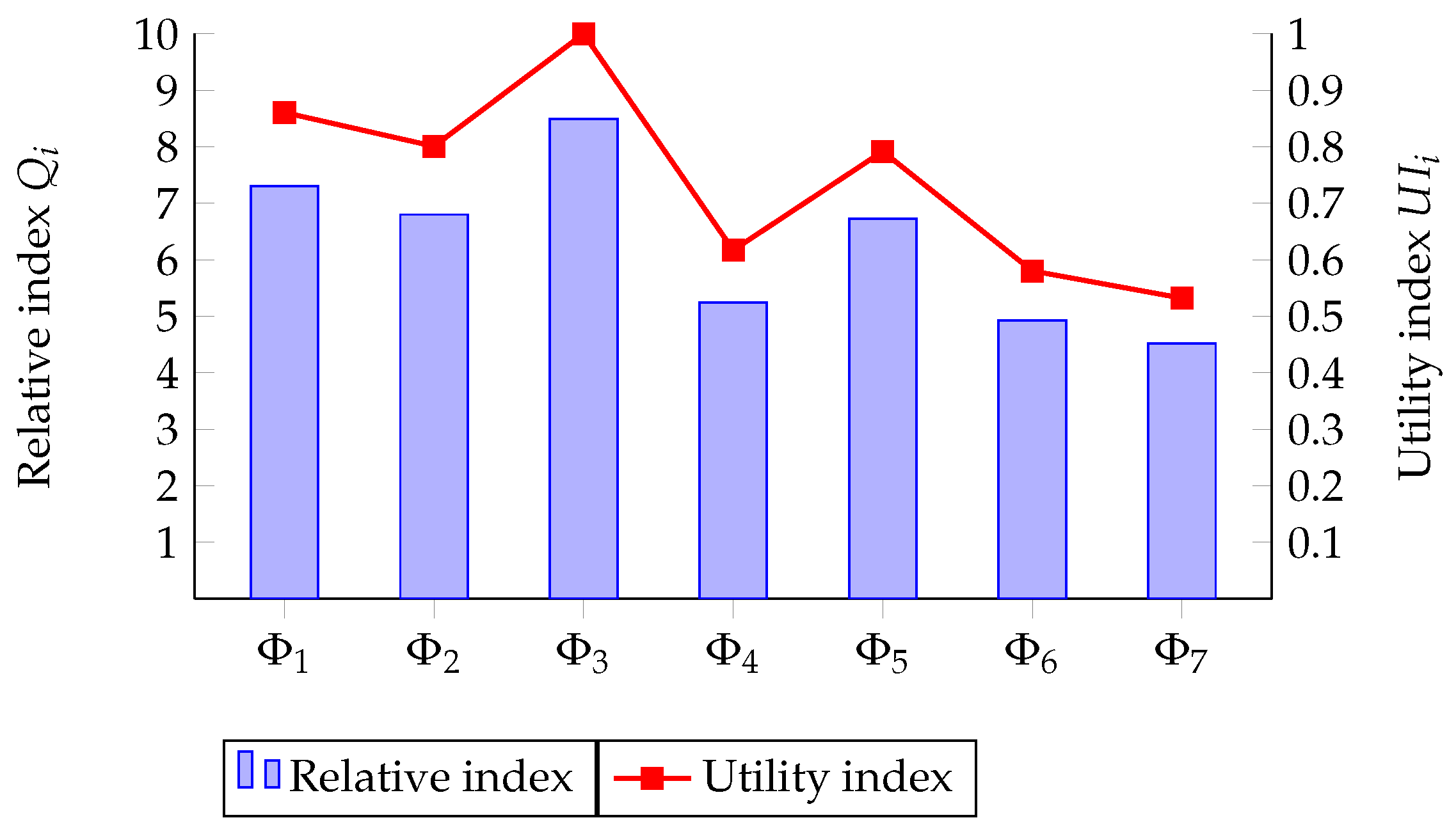
Step 4: The relative index Q i for Φ i is determined by either Equation (37) or (38), with the coefficient ϕ = 0.7 assigned to emphasize beneficial criteria. Subsequently, the utility index U I i for each alternative is computed according to Equation (39). Based on U I i , the seven operational models of urban smart farms are ranked in Table 5. Figure 2 provides a more intuitive presentation of the experimental results.
Table 5 and Figure 2 show that among various operating models of urban smart farms, Rooftop Urban Agriculture ( Φ 3 ) is the smart farm model with the best comprehensive evaluation and is most suitable for the development of urban agriculture.

6.3. Parameter Analysis

This section provides an analysis of the parameters defined in the experimental framework. The entire experimental process incorporates multiple adjustable parameters ( p , q , s , t , ϕ ).
During the construction of the p,q-RTOF decision matrix B, p and q are applied under the constraint 0 ω ξ p + υ ξ q 1 . A higher value of p increases the relative weight of larger input values, thus amplifying the effect of beneficial criteria and penalizing non-beneficial ones more severely. Conversely, a larger q emphasizes the impact of smaller values, leading to a more conservative assessment of the alternatives. In the analysis of parameter p and q, one of them is kept constant while the other is changed. The corresponding results are presented in Table 6 and Table 7. Analyzing Table 6 and Table 7, it can be concluded that Φ 3 demonstrates consistently robust performance across all combinations of parameters p and q, underscoring its stability under diverse decision preferences. In contrast, Φ 1 and Φ 5 exhibit enhanced performance with increasing q values, suggesting their greater suitability for optimistic or benefit-oriented decision-making contexts.
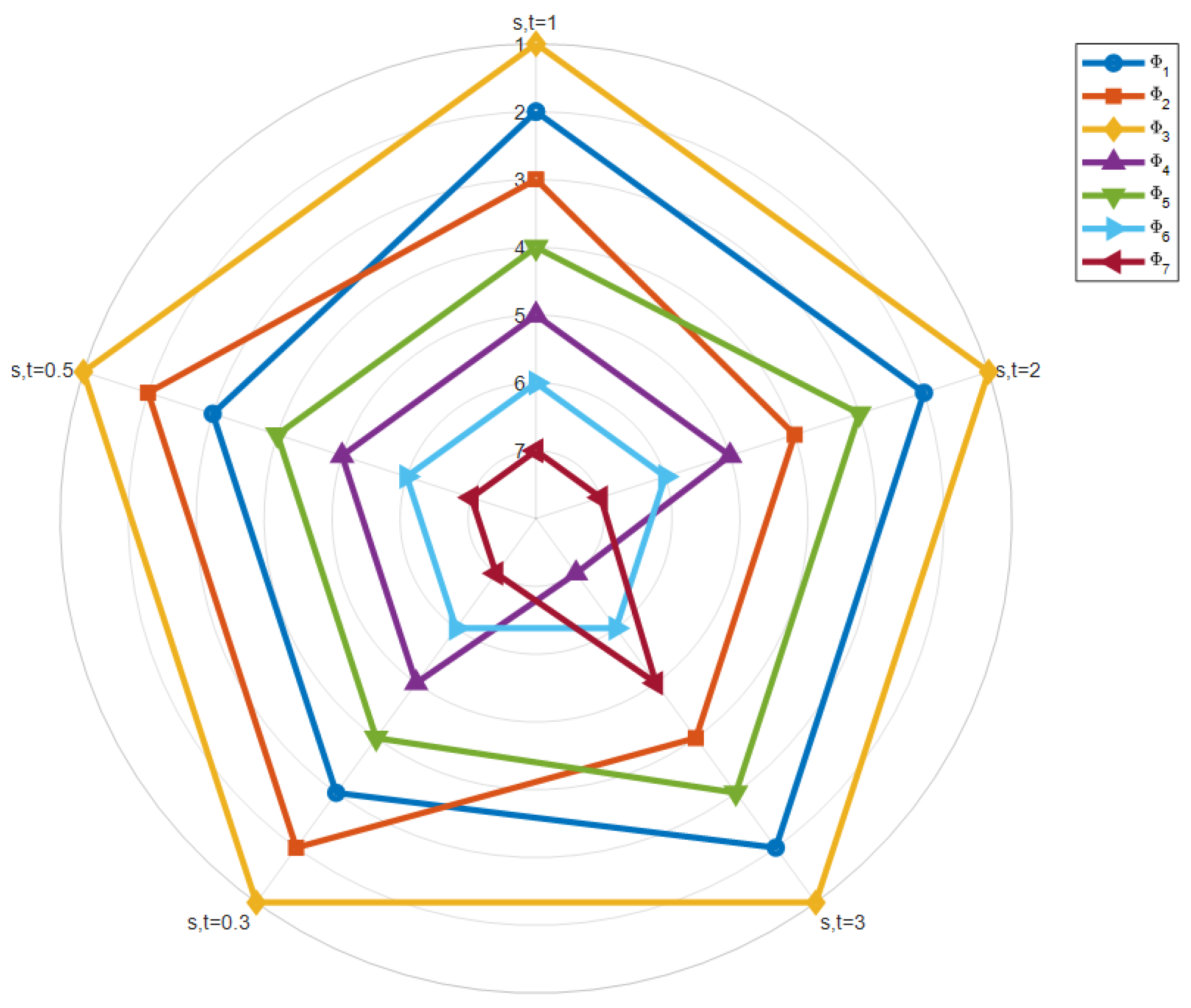
For each alternative, the p,q-RTOFWPBM operator aggregates benefit and cost criteria independently. Within this operator, s and t are important in controlling aggregation bias and regulating the degree of interaction among variables. When s , t > 1 , the impact of outliers is amplified, making the aggregation results more susceptible to dominance by larger values. In contrast, when 0 < s , t < 1 , the variation among extreme values is compressed, leading to more stable outputs and improved robustness of the aggregation process. The analysis results of parameters s and t are presented in Table 8 and Figure 3. As observed, Rooftop Urban Agriculture ( Φ 3 ) consistently emerges as the optimal alternative across all parameter configurations, demonstrating a clear performance advantage. While the overall ranking remains relatively stable, the positions of mid-ranked alternatives exhibit greater sensitivity to variations in the parameter values. As s and t increase, most alternatives tend to decline in their utility index, particularly the less efficient ones such as Φ 4 , Φ 6 and Φ 7 , which experience a more pronounced deterioration. This indicates that under more stringent evaluation conditions, the performance gap between these alternatives and the optimal solution becomes more evident.
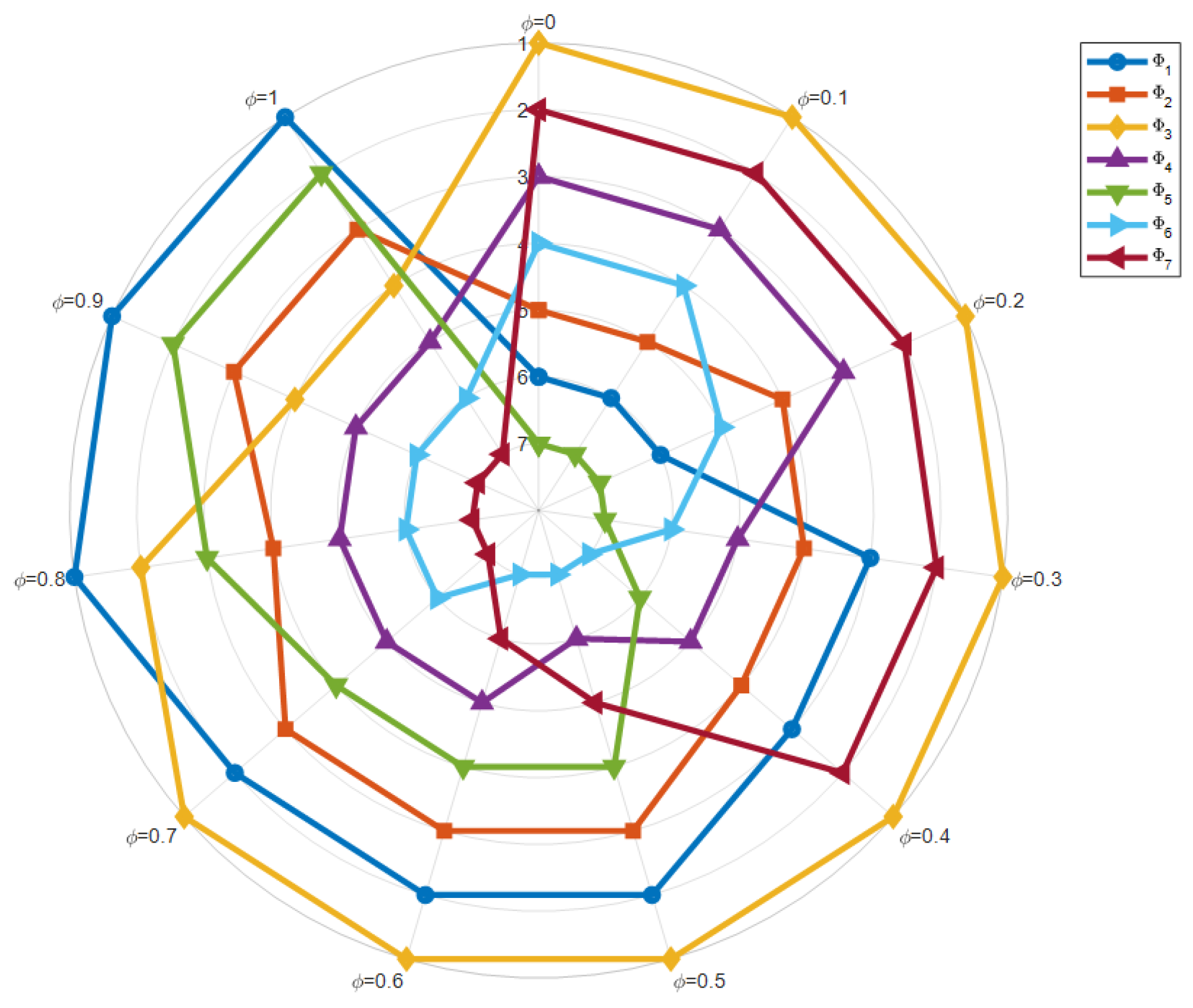
In the p,q-RTOF-PBM-COPRAS method, the parameter ϕ is employed to aggregate the beneficial and non-beneficial components when computing the relative index of alternatives, as shown in Equations (37) and (38). A value of ϕ > 0.5 reflects a decision-making preference toward performance enhancement, whereas ϕ < 0.5 indicates a greater emphasis on cost minimization. The analysis results of parameter ϕ are presented in Table 9, with the corresponding ranking variations in Figure 4.
Notably, Φ 7 exhibits strong performance at lower ϕ values but declines significantly as ϕ increases, indicating a relative advantage in cost-dominated decision-making scenarios. This can be attributed to the fact that the Greenwall High Rise Building ( Φ 7 ) receives low (L), medium–low (ML), very low (VL), and average (A) ratings under the cost-based criteria: Digital Adaptation Cost ( Θ 2 ), Financial Investment ( Θ 3 ), Technological Complexity ( Θ 4 ), and Land Requirement ( Θ 5 ), respectively. In other words, Φ 7 is rated poorly across all negative criteria, which explains why, in decision-making processes, a greater proportion of cost-based criteria makes its superiority more pronounced.
When ϕ 0.7 , Φ 3 consistently ranks highest, indicating strong robustness. For ϕ 0.8 , however, it is overtaken by Φ 1 and Φ 5 . This shift suggests that Φ 1 and Φ 5 outperform Φ 3 under the benefit-based criteria of Technological Compatibility ( Θ 1 ), Crop Diversity ( Θ 6 ), and Crop Intensity ( Θ 7 ), making them better suited to optimistic decision-making scenarios. Nevertheless, cost remains an important factor in all decision-making contexts. Overall, Φ 3 emerges as the most robust option.

6.4. Comparative Analysis

We provide a more extensive contradistinction with existing methods to further validate the p,q-RTOF-PBM-COPRAS method, emphasizing its novelty and effectiveness. Chen et al. [30] used T-SF to represent the initial decision information. The weights of each criterion were calculated using the MEREC, an objective weighting method. Pandey et al. [34] and Mishra et al. [35] used COPRAS as the method framework. Regarding decision information, Pandey et al. employed the traditional Pythagorean fuzzy number (PFN), whereas Mishra et al. used the IVHFFS. Regarding weighting methods, Pandey et al. applied the subjective SWARA, whereas Mishra et al. employed a simple objective weighting method. Karaaslan et al. [36] integrated the TOPSIS method within the IVpqr-SF environment and retained the subjective weighting approach. Li et al. [37] used the IT2TrFS as the expression form of the initial decision information. In the weighting process, AHP and EWM were used for different weighting, respectively, to obtain a reasonable combination weight. Ameen et al. [38] utilized the B p q r SFS to model uncertain information, integrating it with the TOPSIS method as the decision-making framework. In the weighting stage, decision makers directly assign subjective weights to each attribute.
The comparison results are shown in Table 10, and the comparison of the fuzzy environments involved in these methods is shown in Table 11. From the ranking in Table 10, it is evident that four methods still choose Rooftop Urban Agriculture ( Φ 3 ) as the optimal operation mode of urban smart farms. Only two methods judge that Entire Building Glass Greenhouse Type Smart Farm ( Φ 1 ) is the optimal mode, and in the ranking of these two methods, Φ 3 is ranked second only to the optimal choice. Moreover, among all methods, Greenwall High Rise Building ( Φ 7 ) and Suburban Smart Farm ( Φ 6 ) are ranked in the middle and below. Comprehensive analysis shows that the proposed method is effective.
As shown in the comparison in Table 11, p,q-RTOF performs well in key dimensions such as high-order fuzzy expression ability, flexibility and adjustability, and resistance to information loss; it also has obvious comprehensive advantages. On the one hand, its adjustable parameters p,q realize the flexible adjustment of the model in tolerance and fuzziness control. On the other hand, the language expression structure combined with triangular fuzzy numbers is better for complex multi-expert decision environments. In addition, while maintaining strong expressive power and scalability, its computational complexity remains at a medium level, achieving a good balance between expressiveness and operability.
Compared with common MCDM methods such as TOPSIS [36] and PROMETHEE [37], the use of COPRAS makes the proposed method have the advantages of clear modeling structure and strong sorting stability. It can consider the influence of maximization and minimization indicators at the same time through proportional calculation and is suitable for decision-making problems where cost and benefit coexist. Compared with Pandey et al. [34] and Mishra et al. [35], who also used COPRAS as the methodological framework, the proposed method makes significant innovations in weighted aggregation. By combining PA and BM operators, a new p,q-RTOFWPBM operator is proposed as an aggregation operator. Compared with the weighted average operator used by Pandey et al. [34] and Mishra et al. [35], the p,q-RTOFWPBM operator provides enhanced aggregation capabilities and can model the attitudes of decision makers and reduce the impact of extreme values. The p,q-RTOFWPBM operator can capture pairwise interactions between criteria, which are often ignored in linear models such as weighted average operators. These features provide greater flexibility and realism, especially in uncertain or interdependent decision-making environments.
The subjective weighting method may introduce subjective bias when reflecting expert knowledge and preferences. The objective weighting method relies on the distribution characteristics of the data itself but may ignore the intention of the decision maker. Therefore, the combined weighting method that integrates the two can effectively improve the scientificity and rationality of weight setting. Even though Li et al. [37] used the combined weighting method in decision-making, they still chose a simpler weight calculation method such as AHP. The proposed method designs a combined entropy calculation method for p,q-RTOFN to calculate the objective weights, then uses FUCOM to calculate the subjective weights. Finally, the simulated annealing Algorithm 1 is used to iterate the optimal weights as the combined weights applicable to the experiment. This method enhances the robustness of weight allocation, offers strong interpretability and reproducibility, and facilitates application across diverse domains.
Comparison with these methods validates the effectiveness of the p,q-RTOF-PBM-COPRAS method and highlights its performance advantages.

7. Conclusions

The paper introduced a new MCDM within the p,q-rung triangular orthopair fuzzy environment to address inherent uncertainty and complexity. To capture and express fuzzy information more effectively, we introduced a new fuzzy representation, the p,q-RTOFN, which integrated the expressive power of TFS with the flexibility of p,q-ROFS, thereby improving decision accuracy. To enhance fuzzy information aggregation, we integrated the strengths of BM and PA operators to develop the p,q-RTOFWPBM operator. Furthermore, we embedded the p,q-RTOFN and p,q-RTOFWPBM operators into the COPRAS framework, resulting in a new MCDM method termed p,q-RTOF-PBM-COPRAS. A case study on the selection of operating models for urban smart farms verified the effectiveness and applicability of the proposed method. The results demonstrated that the p,q-RTOF-PBM-COPRAS method offers more reliable decision support in uncertain environments.
The contributions of this article include the design of the p,q-RTOFN, the development of hybrid BM and PA aggregation operators within the p,q-RTOF environment, and the integration of these components into the COPRAS method. These contributions expand the fuzzy decision-making toolbox and open new avenues for further theoretical advancement and practical application.
The proposed p,q-RTOF-PBM-COPRAS method also has some limitations. While its application in the context of smart agriculture evaluation was validated, its use in other decision-making contexts needs to be further explored. The use of a single approach for determining p and q in the p,q-RTOFN may limit its adaptability to different decision-making contexts. The computational complexity of the p,q-RTOFWPBM operator may become significant in large-scale problems with numerous criteria and alternatives.
In future research, we plan to explore parameter optimization techniques for p and q to enhance the robustness. This method is applicable to diverse fields including medical resource allocation, sustainable supply chain management, and environmental policy evaluation in order to assess its robustness and adaptability. Additionally, incorporating other advanced aggregation operators or hybridizing the method with machine learning models could further improve its predictive power and decision-making accuracy under conditions of high uncertainty.

Author Contributions

Conceptualization, S.Q.; methodology, S.Q.; software, S.Q.; validation, S.Q.; formal analysis, S.Q.; investigation, S.Q.; resources, X.K.; data curation, S.Q.; writing—original draft preparation, S.Q.; writing—review and editing, X.K.; visualization, S.Q.; supervision, X.K.; project administration, X.K.; funding acquisition, X.K. All authors have read and agreed to the published version of the manuscript.

Funding

This research was funded by the National Natural Science Foundation of China (11371174, 11301227).

Data Availability Statement

The numerical simulation data used to support the findings of this study are included within the article.

Acknowledgments

During the process of completing this paper, I received help and support from many people. Here, I express my sincere gratitude to all the teachers, classmates, relatives and friends who gave me guidance and help. I especially thank my supervisor, Xiangzhi Kong, for valuable guidance and support during the research process. Every discussion and exchange, you have pointed me in the right direction.

Conflicts of Interest

The authors declare no conflicts of interest.

Nomenclature

N * Set of all nonzero natural numbers { 1 , 2 , 3 , } .
R Set of all real numbers.
R + Set of non-negative real numbers.
μ Membership degree.
ν Non-membership degree.
IFSIntuitionistic fuzzy set.
q-ROFSq-rung orthopair fuzzy set.
p,q-ROFSp,q-rung orthopair fuzzy set.
TFNTriangular fuzzy number.
p,q-RTOFNp,q-rung triangular orthopair fuzzy number.
PBM s , t Power Bonferroni mean.
p,q-RTOFPBMp,q-rung triangular orthopair fuzzy power Bonferroni mean.
p,q-RTOFWPBMp,q-rung triangular orthopair fuzzy weight power Bonferroni mean.
T-SFT-spherical fuzzy.
PFNPythagorean fuzzy number.
IVIFSInterval-valued intuitionistic fuzzy set.
IVHFFSInterval-valued hesitant fermatean fuzzy set.
IVpqr-SFNInterval-valued (p,q,r)-spherical fuzzy number.
IT2TrFSInterval type-2 trapezoidal fuzzy set.
B p q r SFSp,q,r-spherical fuzzy set.
TOPSISTechnique for order preference by similarity to ideal solution.
AHPAnalytic hierarchy process.
EWMEntropy weight method.
COPRASComplex proportional assessment
SWARAStep-wise weight assessment ratio analysis.
FUCOMFull consistency method.
MERECMethod based on the removal effects of criteria

References

  1. Alcantud, J.C.R.; Stojanović, N.; Djurović, L.; Laković, M. Decision-Making and Clustering Algorithms Based on the Scored-Energy of Hesitant Fuzzy Soft Sets. Int. J. Fuzzy Syst. 2025. [Google Scholar] [CrossRef]
  2. Mudric-Staniskovski, L.; Djurovic, L.; Stojanovic, N. Energy of a fuzzy soft set and its application in decision-making. Iran. J. Fuzzy Syst. 2024, 21, 35–49. [Google Scholar] [CrossRef]
  3. Sandhya, P.B.; Prashanta, K.P.; Diptirekha, S. Fuzzy TOPSIS technique for multi-criteria group decision-making: A study of crude oil price. Results Control Optim. 2025, 19, 100565. [Google Scholar] [CrossRef]
  4. Sepehr, H.; Ali, E.T.; Sandra, V.; Grit, W. Leading the green charge: A novel type-2 fuzzy VIKOR method applied to eco-conscious freight transport. Expert Syst. Appl. 2025, 285, 128082. [Google Scholar] [CrossRef]
  5. Aslihan, S.; Melisa, C.D.; Alev, T. Assessing collaboration performance of NGOs by a decomposed Fuzzy approach utilizing AHP and COPRAS methods: Turkiye case. Int. J. Disaster Risk Reduct. 2024, 111, 104744. [Google Scholar] [CrossRef]
  6. Rohit, K.; Raj, K.; Kovács, A.; Gusztáv, F.; Tej, S. Thermo-hydraulic characterization and design optimization of delta-shaped obstacles in solar water heating system using CRITIC-COPRAS approach. Energy 2022, 261, 125236. [Google Scholar] [CrossRef]
  7. Muhammad, A.; Kiran, Z.; Muhammet, D. Multi-criteria group decision-making for optimal management of water supply with fuzzy ELECTRE-based outranking method. Appl. Soft Comput. 2023, 143, 110403. [Google Scholar] [CrossRef]
  8. Zadeh, L.A. Fuzzy sets. Inf. Control 1965, 8, 338–353. [Google Scholar] [CrossRef]
  9. Naeem, J.; Jeonghwan, G.; Dragan, P.; Luis, M. Hybrid integrated decision-making model for operating system based on complex intuitionistic fuzzy and soft information. Inf. Sci. 2023, 651, 119592. [Google Scholar] [CrossRef]
  10. Yunus, E.S. Assessment of human factor contribution to risk analysis of chemical cargo shortage incidents by using intuitionistic fuzzy integrated fault tree analysis. Ocean. Eng. 2024, 301, 117559. [Google Scholar] [CrossRef]
  11. Cheng, X.; Cheng, C.; Wang, S. Group decision making with incomplete triangular fuzzy multiplicative preference relations for evaluating third-party reverse logistics providers. Appl. Soft Comput. 2024, 160, 111688. [Google Scholar] [CrossRef]
  12. Dong, J.; Wan, S.; Chen, S.-M. Fuzzy best-worst method based on triangular fuzzy numbers for multi-criteria decision-making. Inf. Sci. 2021, 547, 1080–1104. [Google Scholar] [CrossRef]
  13. Zhang, D.; Hu, J. A novel multi-interval-valued fuzzy set model to solve MADM problems. Expert Syst. Appl. 2024, 238, 122248. [Google Scholar] [CrossRef]
  14. Manisha, M.; Gupta, S.K. On basic arithmetic operations for interval-valued intuitionistic fuzzy sets using the Hamming distance with their application in decision making. Expert Syst. Appl. 2024, 239, 122429. [Google Scholar] [CrossRef]
  15. Ronald, R.Y.; Naif, A. Approximate reasoning with generalized orthopair fuzzy sets. Inf. Fusion 2017, 38, 65–73. [Google Scholar] [CrossRef]
  16. Mijanur, R.S.; Utpal, M. Multiple attribute group decision making based on quasirung orthopair fuzzy sets: Application to electric vehicle charging station site selection problem. Eng. Appl. Artif. Intell. 2022, 115, 105299. [Google Scholar] [CrossRef]
  17. Senapati, T.; Yager, R.R. Fermatean fuzzy weighted averaging/geometric operators and its application in multi-criteria decision-making methods. Eng. Appl. Artif. Intell. 2019, 85, 112–121. [Google Scholar] [CrossRef]
  18. Bonferroni, C. Sulle medie multiple di potenze. Boll. Dell’Unione Mat. Ital. 1950, 5, 267–270. [Google Scholar]
  19. Yager, R.R. The power average operator. IEEE Trans. Syst. Man Cybern. Part A Syst. Hum. 2001, 31, 724–731. [Google Scholar] [CrossRef]
  20. Xu, Z.; Yager, R.R. Some geometric aggregation operators based on intuitionistic fuzzy sets. Int. J. Gen. Syst. 2006, 35, 417–433. [Google Scholar] [CrossRef]
  21. Zhou, X.H.; Yao, J. Triangular fuzzy number intuitionistic fuzzy power averaging operator and its application. Acta Anal. Funct. Appl. 2014, 16, 308–314. [Google Scholar]
  22. Liu, P.; Liu, J.; Chen, S.-M. Some intuitionistic fuzzy Dombi Bonferroni mean operators and their application to multi-attribute group decision making. J. Oper. Res. Soc. 2018, 69, 1–24. [Google Scholar] [CrossRef]
  23. Zhu, B.; Xu, Z.S. Hesitant fuzzy Bonferroni means for multi-criteria decision making. J. Oper. Res. Soc. 2013, 64, 1831–1840. [Google Scholar] [CrossRef]
  24. Zavadskas, E.K.; Kaklauskas, A.; Sarka, V. The new method of multicriteria complex proportional assessment of projects. Technol. Econ. Dev. Econ. 1994, 1, 131–139. [Google Scholar]
  25. Zheng, Y.H.; Xu, Z.S.; He, Y.; Liao, H.C. Severity assessment of chronic obstructive pulmonary disease based on hesitant fuzzy linguistic COPRAS method. Appl. Soft Comput. 2018, 69, 60–71. [Google Scholar] [CrossRef]
  26. Arunodaya, R.M.; Pratibha, R.; Abbas, M.; Kamal, R.P.; Kannan, G.; Melfi, A. Healthcare evaluation in hazardous waste recycling using novel interval-valued intuitionistic fuzzy information based on complex proportional assessment method. Comput. Ind. Eng. 2020, 139, 106140. [Google Scholar] [CrossRef]
  27. Krassimir, T.A. Intuitionistic fuzzy sets. Fuzzy Sets Syst. 1986, 20, 87–96. [Google Scholar] [CrossRef]
  28. Buckley, J.J. Possibilistic linear programming with triangular fuzzy numbers. Fuzzy Sets Syst. 1988, 26, 135–138. [Google Scholar] [CrossRef]
  29. Pamučar, D.; Stević, Ž.; Sremac, S. A New Model for Determining Weight Coefficients of Criteria in MCDM Models: Full Consistency Method (FUCOM). Symmetry 2018, 10, 393. [Google Scholar] [CrossRef]
  30. Chen, Y.-T. An integrated MEREC-taxonomy methodology using T-spherical fuzzy information: An application in smart farming decision analytics. Adv. Eng. Inform. 2024, 62, 102891. [Google Scholar] [CrossRef]
  31. Christoforidou, M.; Borghuis, G.; Seijger, C. Food security under water scarcity: A comparative analysis of Egypt and Jordan. Food Sec. 2023, 15, 171–185. [Google Scholar] [CrossRef] [PubMed]
  32. Boursianis, A.D.; Papadopoulou, M.S.; Panagiotis, D.; Liopa-Tsakalidi, A.; Barouchas, P.; Salahas, G.; Wan, S.; Goudos, S.K. Internet of Things (IoT) and Agricultural Unmanned Aerial Vehicles (UAVs) in smart farming: A comprehensive review. Internet Things 2022, 18, 100187. [Google Scholar] [CrossRef]
  33. Shon, D.; Lee, E.; Lee, Y.; Lee, J.; Byun, N. Characteristics of Smart Farms for Architectural Planning and Design. Buildings 2023, 13, 93. [Google Scholar] [CrossRef]
  34. Bhavna, P.; Manoj, K.K. An integrated Pythagorean fuzzy SWARA-COPRAS framework to prioritise the solutions for mitigating Industry 4.0 risks. Expert Syst. Appl. 2024, 254, 124412. [Google Scholar] [CrossRef]
  35. Arunodaya, R.M.; Peide, L.; Pratibha, R. COPRAS method based on interval-valued hesitant Fermatean fuzzy sets and its application in selecting desalination technology. Appl. Soft Comput. 2022, 119, 108570. [Google Scholar] [CrossRef]
  36. Faruk, K.; Fatih, K. Interval-valued (p,q,r)-spherical fuzzy sets and their applications in MCGDM and MCDM based on TOPSIS method and aggregation operators. Expert Syst. Appl. 2024, 255, 124575. [Google Scholar] [CrossRef]
  37. Li, H.; Yao, X.; Lu, J. Optimal investment decision-making of energy storage technologies on renewable energy generation side based on the Internal Type-2 trapezoidal fuzzy sets-PROMETHEE-II method. Int. J. Electr. Power Energy Syst. 2025, 170, 110861. [Google Scholar] [CrossRef]
  38. Ameen, Z.A.; Salih, H.F.M.; Alajlan, A.I.; Mohammed, R.A.; Asaad, B.A. Enhanced MCDM Based on the TOPSIS Technique and Aggregation Operators Under the Bipolar pqr-Spherical Fuzzy Environment: An Application in Firm Supplier Selection. Appl. Sci. 2025, 15, 3597. [Google Scholar] [CrossRef]
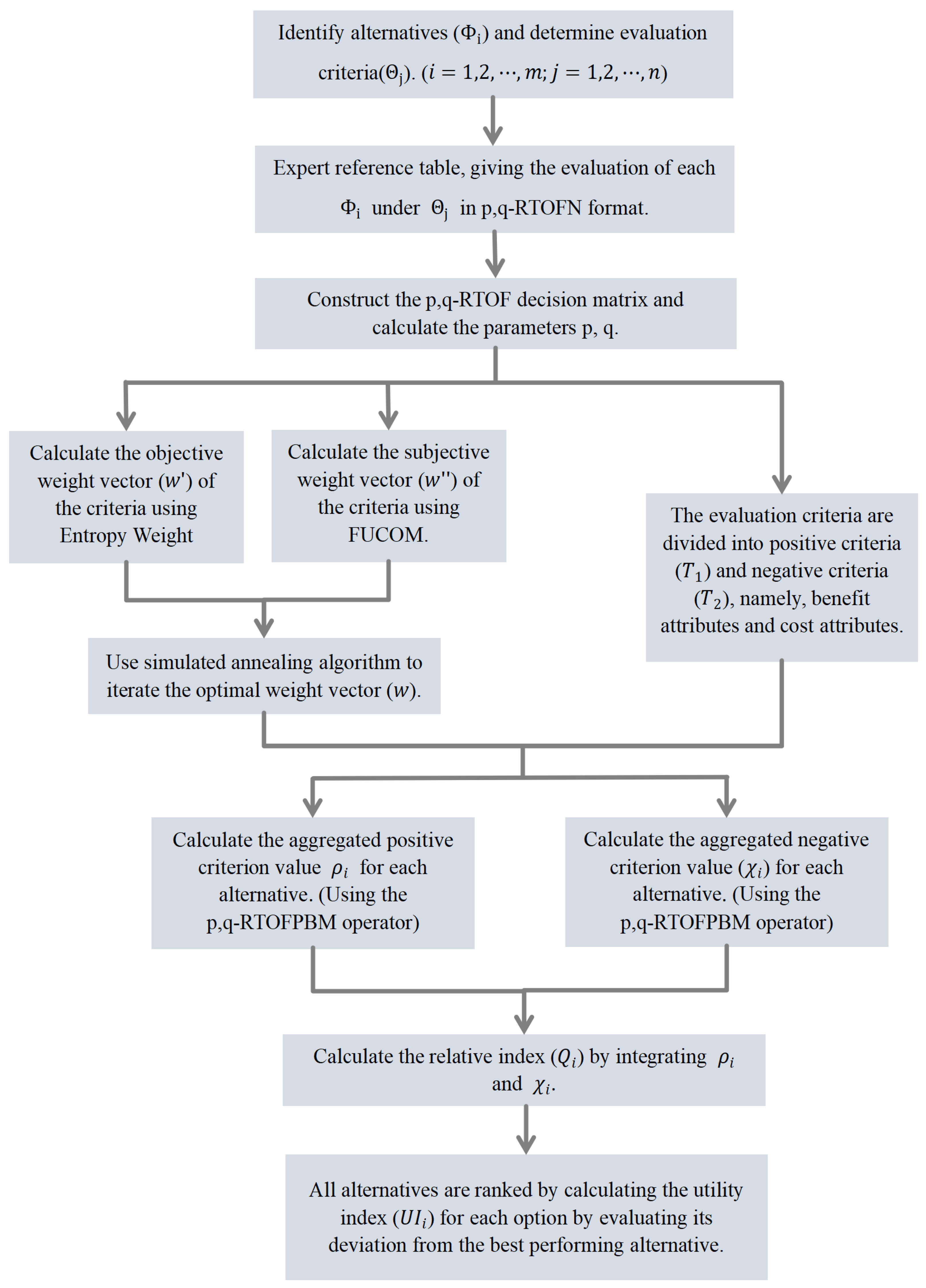
Figure 1. Process of the p,q-RTOF-COPRAS method.
Symmetry 17 01422 g001
Figure 2. Smart farm operational models evaluation result.
Symmetry 17 01422 g002
Figure 3. Impact of parameter s , t on the ranking.
Symmetry 17 01422 g003
Figure 4. Impact of parameter ϕ on the ranking.
Symmetry 17 01422 g004
Table 1. Linguistic scale in p,q-RTOFN form.
Linguistic TermsRelated p,q-RTOFNs
Absolutely High (AH) ( 8.5 , 9.5 , 10.0 ) ; 0.95 , 0.2
Very High (VH) ( 7.5 , 8.5 , 9.5 ) ; 0.85 , 0.35
High (H) ( 6.5 , 7.5 , 8.5 ) ; 0.75 , 0.45
Medium High (MH) ( 5.5 , 6.5 , 7.5 ) ; 0.65 , 0.5
Average (A) ( 4.5 , 5.5 , 6.5 ) ; 0.55 , 0.55
Medium Low (ML) ( 3.5 , 4.5 , 5.5 ) ; 0.5 , 0.65
Low (L) ( 2.5 , 3.5 , 4.5 ) ; 0.45 , 0.75
Very Low (VL) ( 1.5 , 2.5 , 3.5 ) ; 0.35 , 0.85
Absolutely Low (AL) ( 1.0 , 1.5 , 2.5 ) ; 0.2 , 0.95
Table 2. The language decision matrix.
Θ 1 Θ 2 Θ 3 Θ 4 Θ 5 Θ 6 Θ 7
Φ 1 LHMHMHAHAH
Φ 2 HAVHHALAH
Φ 3 AVLLALLMHML
Φ 4 MLMLAAAAA
Φ 5 ALHHAHMHAHVH
Φ 6 LMHMHLHVHL
Φ 7 MHLMLVLALVL
Table 3. The p,q-RTOF decision matrix.
Θ 1 Θ 2 Θ 3 Θ 4 Θ 5 Θ 6 Θ 7
Φ 1 ( 1 , 1.2 , 2.5 ) ; 0.5 , 0.6 ( 2.8 , 3.5 , 4 ) ; 0.8 , 0.4 ( 2 , 3.2 , 3.5 ) ; 0.65 , 0.2 ( 2.5 , 3.2 , 4 ) ; 0.65 , 0.5 ( 2 , 2.5 , 3 ) ; 0.65 , 0.55 ( 2.5 , 3.5 , 4 ) ; 0.7 , 0.3 ( 5 , 5.4 , 6 ) ; 0.85 , 0.2
Φ 2 ( 2.8 , 3 , 4.5 ) ; 0.75 , 0.2 ( 2 , 2.5 , 3.2 ) ; 0.55 , 0.5 ( 3 , 4.2 , 4.5 ) ; 0.8 , 0.3 ( 3 , 4 , 4.5 ) ; 0.65 , 0.2 ( 1.2 , 1.5 , 1.7 ) ; 0.15 , 0.9 ( 2.5 , 2.7 , 3 ) ; 0.5 , 0.55 ( 3 , 3.5 , 4.5 ) ; 0.75 , 0.3
Φ 3 ( 2.3 , 2.5 , 3 ) ; 0.6 , 0.5 ( 1 , 1.2 , 2 ) ; 0.3 , 0.85 ( 1.5 , 1.7 , 2 ) ; 0.25 , 0.65 ( 0.5 , 1 , 1.5 ) ; 0.3 , 0.9 ( 1.5 , 2 , 2.3 ) ; 0.45 , 0.75 ( 2 , 2.8 , 3.2 ) ; 0.7 , 0.1 ( 1.5 , 2.5 , 2.7 ) ; 0.55 , 0.65
Φ 4 ( 2.3 , 2.5 , 3 ) ; 0.45 , 0.65 ( 1.6 , 2.5 , 3 ) ; 0.45 , 0.65 ( 2 , 2.5 , 3 ) ; 0.65 , 0.55 ( 2 , 3 , 3.5 ) ; 0.45 , 0.55 ( 2 , 3 , 3.2 ) ; 0.55 , 0.55 ( 2 , 2.5 , 3.5 ) ; 0.6 , 0.55 ( 2.5 , 2.8 , 3.5 ) ; 0.45 , 0.55
Φ 5 ( 0.7 , 1 , 1.2 ) ; 0.25 , 0.9 ( 3.5 , 4 , 4.5 ) ; 0.7 , 0.25 ( 3 , 3.5 , 4.5 ) ; 0.65 , 0.25 ( 4 , 4.5 , 5.5 ) ; 0.9 , 0.1 ( 2 , 3 , 3.5 ) ; 0.7 , 0.55 ( 4.2 , 4.8 , 5 ) ; 0.98 , 0.2 ( 3.6 , 4 , 5 ) ; 0.7 , 0.4
Φ 6 ( 1.8 , 2.2 , 2.5 ) ; 0.35 , 0.8 ( 2 , 2.8 , 4 ) ; 0.6 , 0.3 ( 2.3 , 3 , 3.5 ) ; 0.65 , 0.3 ( 1.2 , 1.7 , 2 ) ; 0.35 , 0.6 ( 3 , 4.2 , 4.5 ) ; 0.65 , 0.45 ( 4 , 4.2 , 4.8 ) ; 0.9 , 0.4 ( 1 , 1.8 , 2.3 ) ; 0.3 , 0.55
Φ 7 ( 2.8 , 3.1 , 3.8 ) ; 0.65 , 0.35 ( 1.5 , 1.8 , 2 ) ; 0.25 , 0.55 ( 2 , 2.3 , 2.5 ) ; 0.5 , 0.55 ( 1 , 1.2 , 1.5 ) ; 0.35 , 0.65 ( 2.3 , 2.5 , 3.5 ) ; 0.55 , 0.5 ( 1.5 , 1.8 , 2 ) ; 0.35 , 0.7 ( 0.8 , 1 , 1.5 ) ; 0.25 , 0.7
Table 4. The aggregated positive and negative criteria.
ρ i χ i
Φ 1 ( 2.7644 , 3.3672 , 4.1699 ) ; 0.6883 , 0.432 ( 2.2289 , 2.9907 , 3.5206 ) ; 0.6673 , 0.4733
Φ 2 ( 2.7127 , 3.013 , 3.8478 ) ; 0.657 , 0.387 ( 2.3358 , 3.1102 , 3.5211 ) ; 0.5908 , 0.5756
Φ 3 ( 1.8366 , 2.5565 , 2.8965 ) ; 0.6091 , 0.5315 ( 0.9518 , 1.329 , 1.7884 ) ; 0.3136 , 0.8197
Φ 4 ( 2.2289 , 2.5722 , 3.3143 ) ; 0.4976 , 0.5996 ( 1.8484 , 2.6634 , 3.0869 ) ; 0.5127 , 0.6196
Φ 5 ( 2.8712 , 3.3091 , 3.7963 ) ; 0.7055 , 0.5441 ( 3.088 , 3.6719 , 4.439 ) ; 0.70179 , 0.4175
Φ 6 ( 2.0191 , 2.6049 , 3.0881 ) ; 0.4887 , 0.6150 ( 1.8398 , 2.5358 , 3.0231 ) ; 0.5308 , 0.4637
Φ 7 ( 1.475 , 1.7371 , 2.1871 ) ; 0.3973 , 0.615 ( 1.4974 , 1.7329 , 2.0998 ) ; 0.4081 , 0.6011
Table 5. Decision result of operational models of urban smart farms.
Φ 1 Φ 2 Φ 3 Φ 4 Φ 5 Φ 6 Φ 7
Q i 7.30666.79928.49015.23836.7234.92564.517
U I i 0.86060.800810.6170.79190.58020.532
Rank Φ 3 Φ 1 Φ 2 Φ 5 Φ 4 Φ 6 Φ 7
Table 6. Results for different p-values.
p , q UI 1 UI 2 UI 3 UI 4 UI 5 UI 6 UI 7 Rank
2 , 3 0.86060.800810.6170.79190.58020.532 Φ 3 Φ 1 Φ 2 Φ 5 Φ 4 Φ 6 Φ 7
3 , 3 0.87630.822610.64740.79830.60830.5613 Φ 3 Φ 1 Φ 2 Φ 5 Φ 4 Φ 6 Φ 7
4 , 3 0.87030.83110.67500.77820.63380.5839 Φ 3 Φ 1 Φ 2 Φ 5 Φ 4 Φ 6 Φ 7
5 , 3 0.860.832310.6840.75620.64180.591 Φ 3 Φ 1 Φ 2 Φ 5 Φ 4 Φ 6 Φ 7
10 , 3 0.84540.834210.68620.72640.64220.5948 Φ 3 Φ 1 Φ 2 Φ 5 Φ 4 Φ 6 Φ 7
50 , 3 0.82210.832710.68020.70560.63270.5887 Φ 3 Φ 2 Φ 1 Φ 5 Φ 4 Φ 6 Φ 7
100 , 3 0.81450.832310.67760.69630.62810.5861 Φ 3 Φ 2 Φ 1 Φ 5 Φ 4 Φ 6 Φ 7
Table 7. Results for different q-values.
p , q UI 1 UI 2 UI 3 UI 4 UI 5 UI 6 UI 7 Rank
2 , 3 0.86060.800810.6170.79190.58020.532 Φ 3 Φ 1 Φ 2 Φ 5 Φ 4 Φ 6 Φ 7
2 , 4 0.90760.832910.68080.85730.65220.5896 Φ 3 Φ 1 Φ 5 Φ 2 Φ 4 Φ 6 Φ 7
2 , 5 0.94390.859510.71980.90080.69720.6270 Φ 3 Φ 1 Φ 5 Φ 2 Φ 4 Φ 6 Φ 7
2 , 7 0.98240.889210.75290.94230.73350.6593 Φ 3 Φ 1 Φ 5 Φ 2 Φ 4 Φ 6 Φ 7
2 , 10 0.99460.896610.76120.95650.74160.6664 Φ 3 Φ 1 Φ 5 Φ 2 Φ 4 Φ 6 Φ 7
2 , 50 0.99680.895610.76160.96070.74170.6660 Φ 3 Φ 1 Φ 5 Φ 2 Φ 4 Φ 6 Φ 7
2 , 100 0.99680.895610.76160.96070.74170.6660 Φ 3 Φ 1 Φ 5 Φ 2 Φ 4 Φ 6 Φ 7
Table 8. The utility index ( U I i ) under different ϕ .
UI 1 UI 2 UI 3 UI 4 UI 5 UI 6 UI 7 Rank
s , t = 0.3 0.96190.971610.89430.92310.87330.8498 Φ 3 Φ 2 Φ 1 Φ 5 Φ 4 Φ 6 Φ 7
s , t = 0.5 0.94390.950310.84270.89360.81660.7907 Φ 3 Φ 2 Φ 1 Φ 5 Φ 4 Φ 6 Φ 7
s , t = 1 0.86060.800810.61700.79190.58020.5320 Φ 3 Φ 1 Φ 2 Φ 5 Φ 4 Φ 6 Φ 7
s , t = 2 0.84330.704110.54450.80860.53560.5296 Φ 3 Φ 1 Φ 5 Φ 2 Φ 4 Φ 6 Φ 7
s , t = 3 0.77230.54110.37890.76120.39180.3961 Φ 3 Φ 1 Φ 5 Φ 2 Φ 7 Φ 6 Φ 4
Table 9. The utility index ( U I i ) under different ϕ .
UI 1 UI 2 UI 3 UI 4 UI 5 UI 6 UI 7 Rank
ϕ = 0 0.22130.243210.31680.16570.29280.4887 Φ 3 Φ 7 Φ 4 Φ 6 Φ 2 Φ 1 Φ 5
ϕ = 0.1 0.27720.292010.34310.22050.31800.4925 Φ 3 Φ 7 Φ 4 Φ 6 Φ 2 Φ 1 Φ 5
ϕ = 0.2 0.34090.347510.37300.28290.34660.4968 Φ 3 Φ 7 Φ 4 Φ 2 Φ 6 Φ 1 Φ 5
ϕ = 0.3 0.41400.411310.40730.35450.37940.5017 Φ 3 Φ 7 Φ 1 Φ 2 Φ 4 Φ 6 Φ 5
ϕ = 0.4 0.49880.485310.44710.43750.41760.5075 Φ 3 Φ 7 Φ 1 Φ 2 Φ 4 Φ 5 Φ 6
ϕ = 0.5 0.59840.572110.49390.53510.46230.5143 Φ 3 Φ 1 Φ 2 Φ 5 Φ 7 Φ 4 Φ 6
ϕ = 0.6 0.71700.675610.54960.65120.51560.5223 Φ 3 Φ 1 Φ 2 Φ 5 Φ 4 Φ 7 Φ 6
ϕ = 0.7 0.86060.800810.61700.79190.58020.5320 Φ 3 Φ 1 Φ 2 Φ 5 Φ 4 Φ 6 Φ 7
ϕ = 0.8 10.92060.96330.67460.93020.63570.5241 Φ 1 Φ 3 Φ 5 Φ 2 Φ 4 Φ 6 Φ 7
ϕ = 0.9 10.91190.79170.63810.93900.60250.4428 Φ 1 Φ 5 Φ 2 Φ 3 Φ 4 Φ 6 Φ 7
ϕ = 1 10.90440.64210.60620.94660.57360.3720 Φ 1 Φ 5 Φ 2 Φ 3 Φ 4 Φ 6 Φ 7
Table 10. Model evaluation results using multiple methods.
CharacteristicsMethod Type
Chen et al. [30] Pandey et al. [34] Mishra et al. [35] Karaaslan et al. [36] Li et al. [37] Ameen et al. [38] Proposed Method
Decision
information
T-SFNsPFNsIVHFFSsIVpqr-SFNsIT2TrFSs B p q r SFSsp,q-RTOFNs
Methodology
framework
TaxonomyCOPRASCOPRASTOPSISPROMETHEETOPSISCOPRAS
Mathematical
measure
Similarity
and
Closeness
Positive score
and
Negative loss
Positive score
and
Negative loss
Distance
measure
Preference
Measure
Distance
measure
p,q-RTOFWPBM
operator
and
Proportional
Aggregation
Weighting
method
MERECSWARADiscrimination
weight
method
Score
weighting
method
AHP
and
EWM
Directly
from
decision
makers
FUCOM
and
EWM
Weigh typeObjective
weight
Subjective
weight
Objective
weight
Subjective
weight
Combination
weight
Subjective
weight
Combination
weight
Ranking Φ 3 Φ 1
Φ 4 Φ 7
Φ 6 Φ 2 Φ 5
Φ 3 Φ 1
Φ 6 Φ 2
Φ 4 Φ 5 Φ 7
Φ 3 Φ 1
Φ 2 Φ 5
Φ 4 Φ 7 Φ 6
Φ 1 Φ 3
Φ 4 Φ 7
Φ 6 Φ 2 Φ 5
Φ 3 Φ 7
Φ 1 Φ 2
Φ 4 Φ 6 Φ 5
Φ 1 Φ 3
Φ 7 Φ 5
Φ 2 Φ 4 Φ 6
Φ 3 Φ 1
Φ 2 Φ 5
Φ 4 Φ 6 Φ 7
Best model Φ 3 Φ 3 Φ 3 Φ 1 Φ 3 Φ 1 Φ 3
Table 11. Comparison of different fuzzy numbers.
CharacteristicsFuzzy Numbers
T-SFN PFN IVHFFN IVpqr-SFN IT2TrFN B pqr SFN p,q-RTOFN
High-order fuzzy abilityGeneralNoneStrongGeneralStrongStrongStrong
Flexibility and adjustabilityMediumLowHighHighLowHighHigh
Resistance to information lossMediumWeakStrongStrongStrongStrongStrong
Expressive abilityGeneralGeneralStrongGeneralStrongStrongStrong
Language approximation abilityMediumLowHighHighHighMediumHigh
Structural scalabilityLowExtremely HighLowHighLowGeneralHigh
Computational complexityMediumLowHighHighExtremely HighHighMedium
Disclaimer/Publisher’s Note: The statements, opinions and data contained in all publications are solely those of the individual author(s) and contributor(s) and not of MDPI and/or the editor(s). MDPI and/or the editor(s) disclaim responsibility for any injury to people or property resulting from any ideas, methods, instructions or products referred to in the content.