A Decoupled Contrastive Learning Framework for Backdoor Defense in Federated Learning

Abstract

Federated learning (FL) enables collaborative model training across distributed clients while preserving data privacy by sharing only local parameters. However, this decentralized setup, while preserving data privacy, also introduces new vulnerabilities, particularly to backdoor attacks, in which compromised clients inject poisoned data or gradients to manipulate the global model. Existing defenses rely on the global server to inspect model parameters, while mitigating backdoor effects locally remains underexplored. To address this, we propose a decoupled contrastive learning–based defense. We first train a backdoor model using poisoned data, then extract intermediate features from both the local and backdoor models, and apply a contrastive objective to reduce their similarity, encouraging the local model to focus on clean patterns and suppress backdoor behaviors. Crucially, we leverage an implicit symmetry between clean and poisoned representations—structurally similar but semantically different. Disrupting this symmetry helps disentangle benign and malicious components. Our approach requires no prior attack knowledge or clean validation data, making it suitable for practical FL deployments.

1. Introduction

By enabling decentralized model optimization without sharing raw data, federated learning (FL) effectively preserves the privacy of participating clients and enhances the capability for collaborative learning across devices [1]. However, this architecture also creates vulnerabilities that can be exploited by backdoor attacks, in which compromised clients introduce malicious modifications to manipulate the behavior of the global model and undermine the trustworthiness of the entire system. Existing studies indicate that backdoor attacks in FL mainly arise from two types of strategies: the first involves manipulating local training data by injecting samples embedded with specific triggers, thereby implanting hidden malicious behaviors without affecting the model’s performance on the primary task [2,3,4]; the second involves directly tampering with model updates after local training, such as forging or modifying gradients or model parameters to achieve malicious objectives [5,6,7,8]. Both strategies can stealthily affect the behavior of the aggregated global model, posing severe security threats to federated learning systems.

Existing defenses against backdoor threats in federated learning can be broadly categorized into two main approaches: one focuses on enhancing the aggregation mechanism to resist malicious updates [9,10,11], while the other aims to identify and filter out suspicious client models [12,13,14,15], primarily relying on the analysis of plaintext model parameters. These methods attempt to detect potential backdoor attacks by identifying abnormal changes in model weights or gradients. Typically, such approaches assume that the aggregation server is honest and trustworthy [16,17,18,19], or they rely on access to a large amount of clean data on the server side [13,20]. However, these assumptions pose significant risks and contradict the core principle of data localization in federated learning. Prior studies [21,22] have shown that adversaries can exploit model parameters or gradient updates to infer local data of clients, thereby compromising data privacy. Although homomorphic encryption can enhance privacy protection by concealing client data, it introduces new challenges—most notably, the server loses the ability to verify whether received model updates have been maliciously tampered with. This highlights a fundamental trade-off between user privacy and system-level security. Consequently, there is an urgent need to develop robust defense strategies tailored to the unique characteristics of federated learning environments.

We propose a contrastive learning–based defense for federated learning that disentangles clean and backdoor feature representations. In contrast to many existing defense approaches, the proposed method operates without relying on prior knowledge of the attack or the availability of clean validation data, thereby enhancing its practicality and generalizability across diverse federated learning scenarios. Guided by symmetry theory—which suggests clean and poisoned features share structural similarities despite distinct semantics—we design contrastive objectives to break this symmetry and achieve effective separation. Potentially compromised clients are modeled with specialized backdoor detectors, while benign models use contrastive loss, sample reweighting, and the information bottleneck principle to reinforce clean feature learning. This symmetry-informed strategy improves robustness, preserves user privacy by avoiding server-side weight inspection, and provides a theoretically grounded, interpretable defense. Figure 1 illustrates the workflow. All colors are used for visual distinction only and have no practical meaning.

Our Contributions. To summarize, our key theoretical insights and experimental findings include the following:

• We explore how backdoor-related and benign representations interact by analyzing their separability in the feature space. Building on this insight, we propose a novel defense strategy named Decoupled Contrastive Learning (DCL), specifically crafted to counter backdoor threats in federated learning systems. By designing targeted augmentation methods and crafting informative positive–negative sample pairs, DCL encourages the separation of malicious and benign representations. This method enables local models to focus on extracting clean features while minimizing the influence of backdoor signals in the learned embedding space.
• We conducted evaluations on the MNIST, Fashion-MNIST, and CIFAR-10 datasets to validate the performance of our method. Results demonstrate that it reliably suppresses the attack success rate (ASR) below 16% across both transient and sustained backdoor threat settings, all while preserving the primary task accuracy (ACC) with negligible impact.
• We develop a defense-aware adaptive attack strategy and demonstrate that DCL remains robust under such challenging conditions.
• By comparing the communication overhead per training round with and without DCL, we verify that the proposed scheme enhances security without introducing significant communication burden.
• Unlike many existing defenses, our method does not require prior knowledge of the attack or access to clean validation data, and it avoids inspecting client model weights on the server side, which helps better preserve user privacy, making it broadly applicable.

The organization of the remainder of this paper is as follows: Section 2 introduces the background and related works. Section 3 presents the threat model. Section 4 details the design and implementation of the proposed method. Section 5 provides the experimental setup and results. Finally, Section 6 concludes the paper and outlines future work.

2. Related Work

2.1. Backdoor Attacks

Data-Poisoning Attacks. Data-poisoning attacks are a prevalent form of backdoor threat in federated learning, where adversaries intentionally tamper with local training data to cause the global model to behave incorrectly. For example, Shejwalkar [4] introduced an attack based on flipping labels. Expanding on this, Tolpegin [3] examined how variables such as the fraction of malicious participants, the specific class changes, and the timing of their involvement influence the attack’s success. Additionally, Xie [2] broke down the trigger into several localized patterns distributed across different compromised clients, enhancing the attack’s stealthiness and making detection more challenging.

Model-Poisoning Attacks. Adversarial participants may intentionally manipulate local training to inject hidden triggers into the global model, thereby corrupting its behavior without raising suspicion. Bagdasaryan [5] introduced an approach where adversaries locally train a model with embedded backdoors that subtly align with the global model’s parameters, allowing for seamless replacement without triggering anomalies. Fang [6] constructed deceptive gradient updates that can evade existing defense mechanisms, enabling backdoor injection under the guise of legitimate learning. Bhagoji [8] utilized an alternating minimization method to stealthily optimize attack objectives while maintaining plausible update behavior. Sun [7] presented the Distance-Aware Attack, which strategically adjusts feature representations to enhance the effectiveness of targeted poisoning without raising suspicion.

2.2. Backdoor Defense

Robust Aggregation. Robust aggregation techniques are designed to reduce the influence of adversarial updates on the federated global model. Instead of relying on standard averaging, these methods apply aggregation strategies that are resilient to manipulated contributions. For instance, Yin’s $\alpha$-trimmed mean [9] enhances resilience by discarding extreme values during aggregation. Pillutla [10] adopted the geometric median as a robust central tendency measure to limit the effect of poisoned updates. To defend against corrupted updates, Blanchard [11] introduced Krum, an aggregation strategy that selects a client model whose parameters exhibit minimal discrepancy from the majority, thus reducing the influence of outliers. Zhang et al. [18] designed a fine-grained removal strategy to eliminate malicious weights. Huang et al. [16] calibrated anomalous parameters using Fisher information to enhance robustness.

Anomalous Model Detection. Anomalous Model Detection, often known as clustering-based detection, is a widely used strategy for defending against backdoor threats in federated learning. For example, Ding et al. [17] proposed suppressing backdoor behavior by adjusting the weight updates of low-activation neurons. Lin et al. [19] identified potential backdoored models by analyzing layer-wise discrepancies in a fine-grained manner. Shen [12] explored grouping the model updates into clusters based on similarity, allowing suspicious updates that deviate from the main distribution to be identified and flagged as potential threats. Fung [13] introduced FoolsGold, which mitigates adversarial influence by evaluating the consistency patterns in update behaviors across clients. Mu noz-Gonz’alez [14] proposed an adaptive aggregation framework that incorporates statistical consistency checks based on gradient directions to exclude suspicious updates. In a similar vein, Wang [15] designed FLARE, which inspects latent feature distributions to pinpoint and suppress potential poisoning attacks.

2.3. Contrastive Learning

Given the concealed characteristics of backdoor triggers, the model often fails to effectively separate malicious cues from benign representations, thereby increasing the likelihood of misclassification. In contrast, humans are less affected by such perturbations because they tend to focus on the direct associations of objects rather than irrelevant factors [23]. Inspired by disentangled representation learning [24,25,26], we aim to enable the model to learn representations of only the critical features while discarding backdoor perturbations, thereby enhancing the robustness of federated learning. Contrastive learning has shown substantial success in learning discriminative features by guiding the model to distinguish between semantically similar and dissimilar inputs [27,28,29]. In computer vision, approaches like SimCLR [30] and MoCo [31] generate associated input pairs by applying varying transformations to a single data point, treating them as aligned samples. In contrast, samples originating from unrelated instances are treated as divergent, helping the model build a more structured feature representation. This paradigm has proven effective in enhancing visual understanding tasks such as classification and detection. Similarly, in the NLP domain, SimCSE [32] simulates semantically connected text pairs by perturbing a sentence through strategies like token masking or reordering, which improves sentence-level embedding quality. CCL [33] effectively distinguishes causal features from spurious correlations by incorporating causality-guided contrastive learning, thereby improving the model’s generalization and robustness in complex semantic tasks. In the time-series domain, TS-TCC [34] addresses the issues of false negatives and class imbalance in time-series data by leveraging contrastive learning methods to effectively enhance the model’s representation learning capability under imbalanced and noisy conditions.

Moreover, contrastive learning has also shown distinct strengths in achieving feature disentanglement. For example, Xuan [35] introduced a disentangled contrastive learning framework to tackle the issue of class imbalance in long-tailed distributions. Their method formed positive and negative pairs in a way that guided the model to distinguish inter-class features while enhancing the representation of underrepresented classes. Inspired by this capability, we extend contrastive learning to the realm of federated learning for mitigating backdoor threats. By carefully designing positive and negative feature pairs, the proposed strategy promotes the separation of malicious features from clean representations in the latent space, thus reducing the risk of backdoor manipulation.

3. Threat Model

In this study, we consider a federated learning system consisting of 100 clients. In the single-round attack scenario, 10% of the clients are compromised as malicious participants, while in the continuous attack scenario, 40% of the clients persistently participate in multiple training rounds, injecting malicious updates. These malicious clients attempt to manipulate the global model by poisoning their local training data with backdoor triggers. Specifically, in the single-round attack, malicious clients directly replace their local updates in one training round to rapidly implant the backdoor; in the continuous attack, they continuously inject backdoor-related updates over multiple rounds to progressively strengthen the backdoor effect. Throughout the training process, the server neither accesses the clients’ raw data nor inspects the specific model parameters or gradients, relying solely on aggregating local updates to train the global model. This setup adheres to the privacy-preserving principles of federated learning while also increasing the challenges in designing effective defense strategies.

4. Methodology

In this part, we provide a theoretical foundation for our method and assess its effectiveness within a standard federated learning backdoor scenario. Prior studies [15] have shown that the second-to-last layer of a model captures informative, high-level representations that reflect the model’s focus. Building on this understanding, we incorporate an auxiliary network to assist local training. If the client is benign, this additional model enhances the extraction of relevant features, thereby strengthening the quality of local representations. If the client is malicious, the auxiliary model is intentionally trained as a backdoored model $f_{t^{\prime }}$. Then, for the sample pairs $(X,Y)$ held by the malicious client, we extract the penultimate layer outputs of both $f_{t^{\prime }}$ and the local model $f_t$ as R (backdoor features) and Z (clean features), respectively. During training, contrastive learning is employed to decouple R from Z, followed by a sample-reweighting strategy to guide $f_{t^{\prime }}$ toward learning clean features, thereby mitigating the backdoor effect. Upon completion, the purified model $f_t$ is used in global aggregation. The subsequent sections elaborate on each implementation step in malicious clients.

4.1. Backdoor Model $f_{t^{\prime }}$

Building on previous research [36], this paper recognizes that backdoor samples are more easily learned by the model. To further reinforce the backdoor effect in $f_{t^{\prime }}$, the training of $f_{t^{\prime }}$ is terminated immediately after convergence on the backdoor samples, while $f_{t^{\prime }}$ is switched to evaluation mode during the training of $f_t$. At this stage, $f_{t^{\prime }}$ has exclusively learned the backdoor features and has yet to converge on the clean samples.

4.2. Local Model $f_t$

Building on the decoupling concept introduced by Huang [37], this work formulates the loss function by integrating a variational information bottleneck approach alongside sample weighting. The loss function is expressed as three parts:

$$\left\{\begin{array}{c}\begin{array}{cc}\hfill minI(Z;X)& ➀\hfill \\ \hfill maxI(Z;Y)& ➁\hfill \\ \hfill minI(Z;R)& ➂.\hfill \end{array}\hfill \end{array}\right.$$

(1)

Here, $I(·;·)$ denotes mutual information. The terms labeled ➀ and ➁ together form the information bottleneck loss. Term ➀ limits irrelevant information in the input that does not contribute to the label, helping to filter out noise from unrelated features. Term ➁ encourages the latent representation Z to retain the key information needed for accurate label prediction. Term ➂ measures the dependence between the backdoor feature R and the clean feature Z. Reducing the mutual information between Z and R decreases their dependency, allowing Z to focus on extracting features critical for the task. The detailed calculation process is presented below.

Term ➀. To constrain the irrelevant and redundant information in the input that does not affect the label, thus aiding in filtering noise from unrelated features, $I(Z;X)$ can be rewritten based on the mutual information formula as follows:

$$I(Z;X)=\int \int p(x,z)log{\displaystyle \frac{p\left(z\right|x)}{p\left(z\right)}}dxdz.$$

(2)

In real-world federated learning settings, calculating the marginal distribution $p\left(z\right)$ is challenging. Prior studies [38] suggest approximating $p\left(z\right)$ with a variational distribution $r\left(z\right)$. The Kullback–Leibler divergence provides a metric for the difference between $p\left(z\right)$ and $r\left(z\right)$, calculated as follows:

$$\begin{array}{cc}\hfill D_{KL}(p\left(x\right)\parallel q\left(x\right))& =H\left(p\right(x),q(x\left)\right)-H\left(p\right(x\left)\right)\hfill \\ \hfill & =\int p\left(x\right)log{\displaystyle \frac{1}{q\left(x\right)}}dx-\int p\left(x\right)log{\displaystyle \frac{1}{p\left(x\right)}}dx\hfill \\ \hfill & =\int p\left(x\right)(logp\left(x\right)-logq\left(x\right))dx\hfill \\ \hfill & =\int p\left(x\right)log{\displaystyle \frac{p\left(x\right)}{q\left(x\right)}}dx.\hfill \end{array}$$

(3)

Since the Kullback–Leibler divergence cannot be negative, the inequality below holds

$$\begin{array}{cc}\hfill & D_{KL}(p\left(z\right),r\left(z\right))\ge 0\hfill \\ \hfill & \to \int p\left(z\right)log{\displaystyle \frac{p\left(z\right)}{r\left(z\right)}}dz\ge 0\hfill \\ \hfill & \to \int p\left(z\right)logp\left(z\right)dz\ge \int p\left(z\right)logr\left(z\right)dz\hfill \\ \hfill & \to \int \int p(x,z)logp\left(z\right)dxdz\ge \int \int p(x,z)logr\left(z\right)dxdz.\hfill \end{array}$$

(4)

From the aforementioned inequality, the relationship between $p\left(z\right)$ and $r\left(z\right)$ can be established. Consequently, an upper bound for Equation (2) is obtained.

$$\begin{array}{cc}\hfill I(Z;X)& =\int \int p(x,z)logp\left(z\right|x)-p(x,z)logp\left(z\right)dxdz\hfill \\ \hfill & =\int \int p(x,z)logp\left(z\right|x)dxdz-\int p\left(z\right)logp\left(z\right)dz\hfill \\ \hfill & \le \int \int p(x,z)logp\left(z\right|x)dxdz-\int p\left(z\right)logr\left(z\right)dz\hfill \\ \hfill & =\int p\left(x\right)D_{KL}(p\left(z\right|x)\parallel r\left(z\right))dx.\hfill \end{array}$$

(5)

Assuming the posterior $p\left(z\right|x)$ follows a Gaussian distribution with mean $\mu \left(x\right)$ and diagonal covariance matrix $\mathsf{\Sigma }$ whose diagonal elements are ${\sigma }_1^2$ to ${\sigma }_D^2$, and the prior $r\left(z\right)$ is a standard normal distribution with mean zero and identity covariance matrix I, the KL divergence between the two distributions can be formulated as follows:

$$\begin{array}{cc}\hfill & D_{\mathrm{KL}}(p\left(z\right|x)\parallel r\left(z\right))\hfill \\ \hfill & =\int p\left(z\right|x)log{\displaystyle \frac{p\left(z\right|x)}{r\left(z\right)}}dz\hfill \\ \hfill & =-{\displaystyle \frac{1}{2}}logdet\left(\mathsf{\Sigma }\right)+{\displaystyle \frac{1}{2}}\int p\left(z\right|x)\left({(z-\mu \left(x\right))}^{\top }{\mathsf{\Sigma }}^{-1}(z-\mu \left(x\right))\right.\hfill \\ \hfill & \left.+z^{\top }z\right)dz\hfill \\ \hfill & =-{\displaystyle \frac{1}{2}}logdet\left(\mathsf{\Sigma }\right)+{\displaystyle \frac{1}{2}}\left(\mu {\left(x\right)}^{\top }\mu \left(x\right)+\mathrm{Tr}\left(\mathsf{\Sigma }\right)-D\right)\hfill \\ \hfill & ={\displaystyle \frac{1}{2}}\left(\mu {\left(x\right)}^{\top }\mu \left(x\right)+\mathrm{Tr}\left(\mathsf{\Sigma }\right)-logdet\left(\mathsf{\Sigma }\right)-D\right).\hfill \end{array}$$

(6)

Here, $\mu {\left(x\right)}^{\top }\mu \left(x\right)$ represents the squared length of the mean vector using the ${\ell }_2$ norm, $\mathrm{Tr}\left(\mathsf{\Sigma }\right)$ refers to the total of all diagonal elements within the covariance matrix, and $logdet\left(\mathsf{\Sigma }\right)$ denotes the logarithm of the determinant of the covariance matrix. The symbol D corresponds to the dimensionality of the feature vector.

When the covariance matrix $\mathsf{\Sigma }$ is set to zero, the posterior distribution turns deterministic, causing z to equal $\mu \left(x\right)$ and yielding a fixed embedding. In this scenario, reducing the mutual information between Z and X is equivalent to applying an ${\ell }_2$ norm regularization on z.

Term ➁. The goal of maximizing $I(Z;Y)$ is to ensure that the latent representation Z effectively encodes information relevant to predicting the label Y. This helps the model focus on extracting useful, task-relevant clean features, thereby improving classification performance and defense effectiveness, while reducing the interference of backdoor features on the model’s decisions. Since calculating $I(Z;Y)$ directly is challenging, we approximate it by minimizing the cross-entropy loss ($CE$). To achieve this, a sample-weighted cross-entropy loss ($\mathcal{L}\mathrm{weighted}$) is applied to train $ft$, where features from the intermediate layers of $f_{t^{\prime }}$ are used only for weighting purposes without backpropagation through $f_{t^{\prime }}$. The weight calculation is expressed as follows:

$$\omega \left(x\right)=1-{\displaystyle \frac{CE(f_t\left(x\right),y)}{CE(f_{t^{\prime }}\left(x\right),y)+CE(f_t\left(x\right),y)+ϵ}}.$$

(7)

For training samples, a low loss value on $f_{t^{\prime }}$ results in a weight near 0, while a high loss leads the weight to approach 1. A tiny value $ϵ$ is included to prevent division errors caused by zero denominators. This weighting mechanism aims to direct $f_t$ towards emphasizing clean feature learning and diminishing the influence of backdoor feature extraction. It is important to note that the features of the auxiliary model $f_{t^{\prime }}$ are computed only during the forward pass and do not participate in the backward propagation.

Term ➂. Using the connection between mutual information and entropy, $I(Z;R)$ can be represented as follows:

$$I(Z;R)=H\left(Z\right)-H\left(Z\right|R).$$

(8)

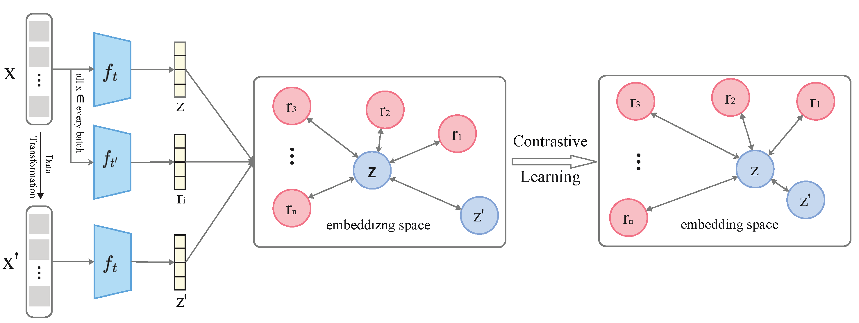
Minimizing the mutual information $I(Z;R)$ aims to separate the clean features Z from the backdoor features R, helping the model focus on extracting task-relevant clean key information while suppressing interference from backdoor features, thereby enhancing the model’s defense capability against backdoor attacks. We utilize contrastive learning to improve the model’s feature space by contrasting positive and negative pairs. Positive pairs include z and $z^{\prime }$, where $z^{\prime }$ is generated by applying data augmentation on the input x to form $x^{\prime }$, which is then processed by the local model $f_t$ to obtain its feature. Negative pairs are constructed from the local model’s feature z and the backdoor model’s feature $r_i$. Figure 2 illustrates the overall contrastive learning framework. All colors are used for visual distinction only and have no practical meaning.

Within this framework, the local model $f_t$ and the backdoor model $f_{t^{\prime }}$ produce intermediate representations z and r, respectively. These outputs are fed into the contrastive learning component to compute the contrastive loss. The loss function employed is based on the InfoNCE formulation, defined as follows:

$$\begin{array}{cc}\hfill & s^{+}=\mathrm{sim}(z,z^{\prime })s_i^{-}=\mathrm{sim}(z,r_i)(i=1,\dots ,n)\hfill \\ \hfill & {\mathcal{L}}_{\mathrm{contrastive}}=-log{\displaystyle \frac{exp\left(s^{+}/\tau \right)}{exp\left(s^{+}/\tau \right)+{\displaystyle \sum _{i=1}^n}exp\left(s_i^{-}/\tau \right)}}.\hfill \end{array}$$

(9)

Here, $\mathrm{sim}(·,·)$ refers to the similarity measure between sample pairs, commonly calculated using cosine similarity; $s^{+}$ denotes the similarity score for positive pairs, whereas $s_i^{-}$ corresponds to that of negative pairs; the parameter $\tau$ regulates the sharpness of the similarity distribution, while n represents the total count of samples.

It is worth noting that the InfoNCE loss serves as a lower bound on the mutual information between positive pairs $I(Z;Z^{\prime })$ [39,40]; thus, maximizing the similarity of positive pairs implicitly maximizes this mutual information. Meanwhile, by contrasting with negative samples $r_i$, the method encourages the dissimilarity between Z and R, effectively reducing the mutual information $I(Z;R)$ and promoting disentanglement. Although InfoNCE does not theoretically guarantee complete independence between Z and R, prior works [41] demonstrate that with sufficient negative samples and appropriate temperature settings, it effectively enforces feature separation in practice. Therefore, we consider the use of the InfoNCE-based contrastive loss as a practical and efficient approach to approximate the desired feature disentanglement in our framework.

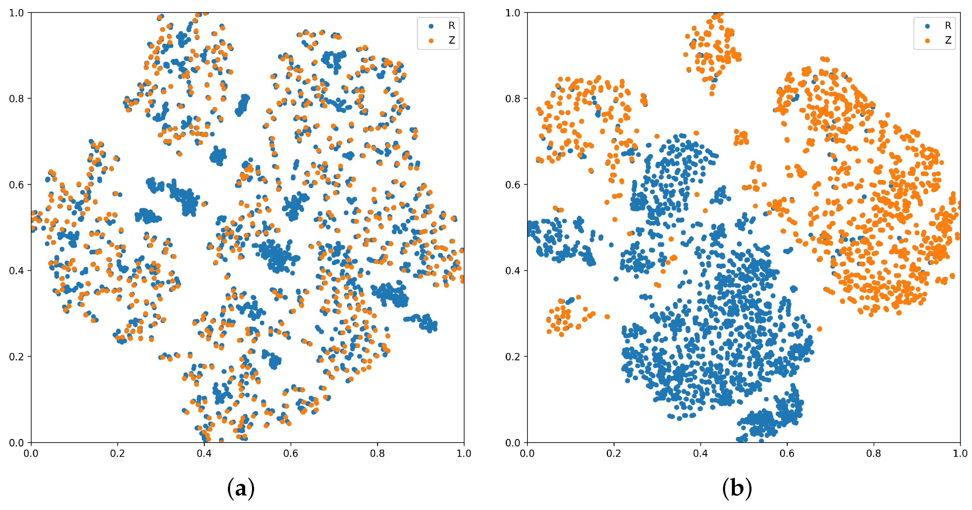
Through optimizing this objective, the model increases similarity between positive pairs to strengthen the consistency of clean features and reduces similarity among negative pairs to lower the mutual information between Z and R. Finally, integrating contrastive learning with sample weighting, the loss function for $f_t$ is formulated as follows:

$${\mathcal{L}}_{\mathrm{C}}={\mathcal{L}}_{\mathrm{contrastive}}+{\mathcal{L}}_{\mathrm{weighted}}+\beta {\parallel \mu \left(x\right)\parallel }_2^2,$$

(10)

$\beta$ controls the strength of regularization, balancing feature compression and model performance. Too small weakens defense; too large harms accuracy. We set $\beta$ = 0.1 in our experiments.

Based on the described approach, stochastic gradient descent optimizes the loss functions for both $f_{t^{\prime }}$ and $f_t$. Algorithm 1 presents the entire procedure. The contrastive learning process is described in Algorithm 2.

Algorithm 1 Decoupled contrastive learning for federated backdoor defense

1: Global server’s input: Global model $f_0$, total communication rounds T, Client sampling size per round K  2: Local client’s input: backdoor model training iterations $T_1$, local model training iterations $T_2$  3: Global output: Global backdoor-free model f  4: Initialize: Global model $f\leftarrow f_0$  5: for each round $t\in \{1,2,\dots ,T\}$ do  6:     Server samples a set of clients ${\mathcal{C}}_t$ with $|{\mathcal{C}}_t|=K$  7:     for each client $k\in {\mathcal{C}}_t$ do  8:         if client k is labeled as malicious then  9:                                    ▷Train backdoor model $f_{t^{\prime }}$ 10:            Initialize $f_{t^{\prime }}$ and local model $f_t\leftarrow f$ 11:            for iteration $i=1$ to $T_1$ do 12:               Train $f_{t^{\prime }}$ using poisoned data via SGD 13:            end for 14:            for iteration $j=1$ to $T_2$ do 15:               Sample poisoned data $(x,y)$ 16:               ${\left\{r_i\right\}}_{i=1}^n\leftarrow \{f_{t^{\prime }}\left(x\right)\mid x\in \mathrm{batch},\forall \mathrm{batch}\in \mathrm{dataset}\}$ 17:               $z\leftarrow f_t\left(x\right)$                       ▷Current feature from clean model 18:               $z^{\prime }\leftarrow f_t\left(x^{\prime }\right)$                                ▷Augmented view 19:               Compute contrastive loss: $\mathrm{Contrastive}\_\mathrm{L}({\left\{r_i\right\}}_{i=1}^n,z,z^{\prime })$ 20:               Compute instance weight $w\left(x\right)$ 21:               Optimize $f_t$ using SGD with total loss (e.g., Equation (10)) 22:            end for 23:         else 24:                                       ▷Benign client training 25:            Initialize local model $f_t\leftarrow f$ 26:            Train $f_t$ using clean data with SGD for $T_2$ iterations 27:         end if 28:         Client k sends updated model $f_t$ to server 29:      end for 30:      Server aggregates models from clients to update f 31: end for

Algorithm 2 Contrastive loss calculation

1: Input: Clean feature z, Augmented clean feature $z^{\prime }$, Set of backdoor features ${\left\{r_i\right\}}_{i=1}^n$, Temperature parameter $\tau$  2: Output: Contrastive loss $L_{\mathrm{contrastive}}$  3: Initialize:  $L_{\mathrm{contrastive}}\leftarrow 0$  4: function Contrastive_L$({\left\{r_i\right\}}_{i=1}^n,z,z^{\prime })$  5:     $\mathrm{sim}(z,z^{\prime })\leftarrow {\displaystyle \frac{z·z^{\prime }}{\parallel z\parallel \parallel z^{\prime }\parallel }}$                          ▷Similarity between z and $z^{\prime }$  6:     for each $r_i\in \{r_1,r_2,\dots ,r_n\}$ do  7:        $\mathrm{sim}(z,r_i)\leftarrow {\displaystyle \frac{z·r_i}{\parallel z\parallel \parallel r_i\parallel }}$                          ▷Similarity between z and $r_i$  8:     end for  9:     $\mathrm{Numerator}\leftarrow exp\left({\displaystyle \frac{\mathrm{sim}(z,z^{\prime })}{\tau }}\right)$ 10:     $\mathrm{Denominator}\leftarrow \mathrm{Numerator}+{\sum }_{i=1}^{n}exp\left({\displaystyle \frac{\mathrm{sim}(z,r_i)}{\tau }}\right)$ 11:     $L_{\mathrm{contrastive}}\leftarrow -log{\displaystyle \frac{\mathrm{Numerator}}{\mathrm{Denominator}+ϵ}}$ 12:     Return: $L_{\mathrm{contrastive}}$

5. Results

This section assesses the effectiveness of DCL against data-poisoning attacks. We compare DCL’s performance with seven leading defense techniques: Krum [11], RFA [10], Median [9], FLTrust [20], DnC [42], SDFC [16], and FLGuardian [43]. Additionally, we provide results for a baseline scenario without any defense mechanisms, denoted as “No Defense”. In addition to adopting the experimental configurations from [2,5], we also design experiments based on the setup used in our theoretical analysis to support its validity. Furthermore, we assess the performance of DCL under adaptive attack scenarios.

5.1. Experimental Settings

Our experiments follow the protocol outlined by Bagdasaryan et al. [5], guided by parameters informed by theoretical insights. The system consists of 100 clients, with 10 clients participating in each training round—6 are benign, and 4 are adversarial. Benign clients use a learning rate of 0.1, while malicious clients adopt 0.05. Training is performed with a batch size of 64 samples per client.

Datasets and DNNs: We assess our method using three widely recognized image classification benchmarks: MNIST [44], Fashion-MNIST (F-MNIST) [45], and CIFAR-10 [46]. An overview of these datasets is presented in

Table 1. Dataset specifications.

Dataset	Labels	Input Size	Training Images
MNIST	10	28 × 28 × 1	60,000
Fashion-MNIST	10	28 × 28 × 1	60,000
CIFAR-10	10	32 × 32 × 3	50,000

. For the MNIST and Fashion-MNIST datasets, the SimpNet architecture [47] is utilized, while ResNet-34 [48] serves as the backbone model for CIFAR-10. To reflect the typical Non-IID distribution in federated learning, we generate data heterogeneity by sampling from a Dirichlet distribution [49] with parameter $\alpha =0.5$.

Attack Setups: We adopted the BadNets [50] attack methodology as the adversarial framework in our experiments. Model optimization was performed using stochastic gradient descent (SGD) on deliberately poisoned training datasets. The proportion of poisoned samples per training batch was strictly set to 20 out of 64 for the MNIST and Fashion-MNIST datasets, and 5 out of 64 for the CIFAR-10 dataset. During training, all backdoor attacks consistently used class 2 as the target label. To provide a more intuitive illustration of the impact of backdoor attacks and the defense effectiveness of our method, we present representative poisoned samples from the MNIST dataset. As shown in Figure 3, the vanilla model is easily influenced by the trigger (located at the top-left corner), tends to prioritize learning the backdoor features, and misclassifies the poisoned samples into the target class.

Evaluation Criteria: We evaluation focuses on two key metrics: the classification accuracy (ACC) reflecting the model’s performance on the main task, and the attack success rate (ASR) measuring the effectiveness of backdoor intrusions. ASR indicates how susceptible the model is to backdoor triggers, with attackers attempting to increase it while defenders strive to reduce it. Meanwhile, ACC evaluates the model’s effectiveness on its primary task, which both attackers and defenders aim to preserve to avoid compromising normal operation.

5.2. Evaluation on Backdoor Mitigation

It is crucial to emphasize that backdoor attacks are executed only after the global model has reached convergence, as previous studies [2] have demonstrated that initiating poisoning from the first training round significantly hinders the model’s convergence on the primary task. In the experimental setup, two distinct attack strategies were examined: single-round and continuous attacks. In a single-round attack, the attacker participates in a single training iteration. Conversely, a continuous attack entails the attacker participating in all training rounds, which is more challenging to counteract.

Single attack: To ensure an unbiased comparison, we report the attack success rate and accuracy of our method and baseline approaches at identical training rounds. The single-step attack results are detailed in

Table 2. Comparison of DCL and leading defenses in terms of robustness under single-attack scenarios on MNIST, FMNIST, and CIFAR-10 datasets using 0.5 degree of non-IID data.

Defense	MNIST		Fashion-MNIST		CIFAR-10
	ACC(%)	ASR(%)	ACC(%)	ASR(%)	ACC(%)	ASR(%)
No Defense	96.33	83.46	81.50	96.79	78.74	80.35
Krum	96.50	0.39	79.75	10.21	77.42	9.13
RFA	96.93	0.43	80.25	5.04	78.84	6.83
Median	96.76	0.37	80.92	6.23	65.77	3.14
FLTrust	96.28	0.48	79.64	7.60	72.65	4.49
Dnc	96.61	0.52	80.33	5.38	76.59	4.98
SDFC	96.62	0.55	79.81	5.13	76.40	5.74
FLGuardian	96.86	0.24	81.51	4.78	74.87	2.23
DCL	96.67	0.18	80.47	4.66	76.53	4.28

. As shown, without any defense, the ASR surpasses 80% on all three datasets, while ACC remains above 78%. Under single-step attacks, traditional defense techniques also achieve notable effectiveness since model replacement leads to abnormal gradient updates that these methods can mitigate. Our proposed DCL method lowers the ASR to under 5% across all datasets, with the drop in ACC kept within 3%. Although DCL’s performance on CIFAR-10 is marginally behind some baselines, its local defense strategy offers the advantage of minimizing privacy risks.

Continuous attack: 

Table 3. Comparison of DCL and leading defenses in terms of robustness under continuous attack scenarios on MNIST, FMNIST, and CIFAR-10 datasets using 0.5 degree of non-IID data.

Defense	MNIST		Fashion-MNIST		CIFAR-10
	ACC(%)	ASR(%)	ACC(%)	ASR(%)	ACC(%)	ASR(%)
No Defense	97.46	99.97	81.27	99.86	78.92	83.64
Krum	96.59	0.21	72.98	20.13	42.40	17.58
RFA	97.54	99.93	82.34	99.87	75.39	65.30
Median	97.14	65.89	83.84	99.90	60.01	70.13
FLTrust	91.96	20.66	74.59	34.46	73.85	63.97
Dnc	91.81	99.78	65.18	98.34	54.32	82.54
SDFC	90.74	99.99	61.42	99.05	52.15	82.73
FLGuardian	90.03	19.63	76.51	36.88	64.81	43.92
DCL	96.69	0.96	77.24	15.71	73.42	10.31

shows the results for continuous attack scenarios. It is clear from the table that most defense methods struggle under continuous attacks. While Krum reduces the ASR on MNIST and Fashion-MNIST to below 21%, its effectiveness on CIFAR-10 remains limited. In contrast, DCL significantly decreases the ASR to very low levels, with the corresponding drop in ACC kept within acceptable bounds. Specifically, the ASR on MNIST falls below 1%, with ACC decreasing by less than 1%. DCL reduces the attack success rate to under 16% on Fashion-MNIST and below 11% on CIFAR-10, with accuracy decreasing by less than 6%. Unlike single-round attacks, continuous attacks introduce backdoors progressively through repeated malicious updates, making them harder to detect and defend. DCL addresses this by isolating backdoor features from clean representations during training, minimizing the impact of poisoned data on local models. This enhances the global model’s resilience, making it more resistant to both one-time and ongoing attacks.

5.3. Hidden-Feature Visualization

In Figure 4, we leverage t-SNE [51] to visualize the latent space, providing a comprehensive understanding of the proposed method. A data-poisoning attack is conducted on the CIFAR-10 dataset. Figure 4a shows the disentanglement capability of the latest baseline method FLGuardian, where the backdoor and clean features largely overlap, indicating poor disentanglement. In Figure 4b, the distributions of R and Z after training by our proposed method are depicted, revealing a clear separation between the two. This observation confirms the successful disentanglement of features achieved by our approach. Figure 4c,d present the t-SNE visualizations of R and Z, respectively, where samples with different labels are represented by distinct colors. Notably, backdoor samples form distinct clusters within R, indicating that the backdoor features have been effectively captured by the model $f_{t^{\prime }}$. Conversely, in Z, backdoor samples are closely aligned with clean samples, demonstrating the effectiveness of DCL in mitigating backdoor attacks and improving the robustness of federated learning systems.

5.4. Consequences of Different Non-IID Degrees

To simulate varying degrees of Non-IID data in federated learning, we employ the Dirichlet distribution with hyperparameter $\alpha$. We assess the effect of a single attack on the CIFAR-10 dataset under both “No Defense” and DCL defense settings. As depicted in Figure 5, without any defense, an increase in $\alpha$ corresponds to a stronger backdoor attack performance. In contrast, our DCL method consistently maintains the ASR below 6% across different Non-IID levels, while ensuring stable classification accuracy on benign data.

5.5. Results of Adaptive Attacks

To evaluate DCL’s robustness against potential adaptive attacks, we design targeted countermeasures and assess its performance in this scenario. The adaptive attack specifically targets DCL’s two defense mechanisms: (1) for feature decoupling, attackers employ dynamic feature obfuscation by minimizing the Wasserstein distance (beyond cosine similarity) between backdoor and clean features in latent space; (2) for contrastive learning, they implement adversarial sample weighting to disguise poisoned samples as high-confidence clean samples during local training. As shown in

Table 4. Adaptive attack evaluation.

Defense	MNIST		Fashion-MNIST		CIFAR-10
	ACC(%)	ASR(%)	ACC(%)	ASR(%)	ACC(%)	ASR(%)
No Defense	97.86	100.00	80.97	99.99	78.61	84.83
DCL	96.52	1.41	74.22	18.46	70.05	12.32

, DCL maintains robust defense performance under continuous adaptive attacks across all datasets.

5.6. Comparison of Computational Overhead

During the local training phase, the proposed method introduces an auxiliary model combined with a contrastive learning mechanism, which inevitably incurs some computational overhead. To evaluate this overhead, experiments were conducted on the MNIST dataset with a non-IID data partition following a Dirichlet distribution parameterized by 0.5. The proposed method was compared against the standard federated averaging algorithm (FedAvg) without defense, focusing on the local training time per communication round. As shown in

Table 5. Computation overhead comparison under different attack scenarios on MNIST dataset using 0.5 degree of non-IID data.

Attack Type	Method	Avg. Local Training Time (s)
Single Attack	No Defense	39
	DCL	42
Continuous Attack	No Defense	129
	DCL	141

, under the single-attack scenario, the average local training time increases by only approximately 7.6% compared to FedAvg. In the more challenging continuous attack scenario, the additional overhead remains controlled at around 9%, without significant growth. These results indicate that the proposed method enhances security without introducing noticeable communication burden. However, we also acknowledge that in large-scale deployments or resource-constrained federated learning environments, requiring each client to train both a contrastive learning model and a variational inference model simultaneously may limit the feasibility of the proposed method. In the future, the algorithm design could be further improved by sharing backdoor model parameters or caching intermediate computation results, thereby enhancing its scalability and practicality in complex real-world scenarios.

5.7. Impact of Temperature Parameter $\tau$ on DCL

To investigate the effect of the temperature parameter $\tau$ in contrastive learning, we conducted experiments on CIFAR-10 under a single-shot attack scenario with $\tau$ set to 0.05, 0.1, and 0.5. The results in

Table 6. Compare the defense effectiveness under different temperature parameters in a Single-shot Attack scenario on the CIFAR-10 Dataset with a non-IID degree of 0.5.

$\mathit{\tau }$	ACC(%)	ASR(%)
0.05	76.53	4.28
0.1	76.41	5.93
0.5	77.26	7.57

show that smaller $\tau$ values sharpen the contrastive loss, enhancing feature separation between clean and backdoor samples, thus improving defense. Larger $\tau$ values smooth the loss and reduce discriminability, weakening defense. Accordingly, we select $\tau$ = 0.05 for subsequent experiments.

5.8. Ablation Study of Contrastive Learning and Information Bottleneck

To evaluate the contributions of each component in our defense framework, we conducted an ablation study on CIFAR-10 under a single-shot attack. We compared three settings: contrastive learning only (CL-only), information bottleneck only (IB-only), and the combined method (DCL). As shown in

Table 7. Ablation study of CL and IB components in the proposed defense framework.

Defense	ACC(%)	ASR(%)
No Defense	78.74	80.35
IB-only	76.55	63.29
CL-only	74.31	15.86
DCL	76.53	4.28

, both CL-only and IB-only significantly reduced the attack success rate (ASR) compared to the baseline, with CL-only achieving a lower ASR of 15.86%. This is because contrastive learning explicitly disentangles features, helping to identify backdoor features even without IB. In contrast, IB alone cannot fully separate clean and backdoor features, resulting in higher ASR. The combined method further reduced ASR to 4.28% while maintaining high clean accuracy, demonstrating that CL and IB complement each other by compressing redundant information and explicitly disentangling features.

We also compared the feature disentanglement capabilities of IB-only and CL-only in more detail. Figure 6a illustrates the disentanglement performance of IB-only, where backdoor and clean features largely overlap. This is mainly because the Information Bottleneck strategy focuses on compressing irrelevant information and extracting key predictive information, resulting in weaker disentanglement ability in the feature space. Figure 6b shows the disentanglement effect of CL-only, where clean and backdoor features are more effectively separated, though some overlap still exists. This is because contrastive learning helps improve the discriminability and separability of features by pulling together samples of the same class and pushing apart samples of different classes.

6. Conclusions

We proposed a federated backdoor defense strategy called decoupled contrastive learning (DCL). Unlike traditional methods that rely on inspecting model updates to detect backdoor attacks—often requiring access to clients’ local data or gradients and risking privacy breaches—DCL implements defense locally, safeguarding data privacy while significantly lowering backdoor attack success rates. Our approach outperforms existing defense techniques in both single-round and continuous attack scenarios. From a theoretical standpoint, DCL utilizes feature disentanglement combined with contrastive learning to strengthen the model’s capacity to extract clean features and suppress backdoor-related ones, thereby improving resilience against diverse attacks. This framework also has potential for extension to other fields, such as natural language processing, supporting its applicability in multimodal tasks. However, the current study validates the proposed method primarily on two architectures, SimpNet and ResNet-34. While these models are representative to some extent, the limited coverage of model types remains a constraint. Moreover, our method is designed for static backdoor attacks; its generalizability to dynamic and more sophisticated attacks requires further investigation. In future work, we plan to extend DCL to a wider range of mainstream and structurally diverse architectures, further optimize communication efficiency to enhance the scalability of the method—such as by sharing the parameters of the backdoor model or caching intermediate computation results—and strengthen its robustness against more sophisticated backdoor strategies (e.g., dynamic attacks). Additionally, we will focus on addressing technical and resource constraints, integrating advanced feature disentanglement defenses, expanding experimental baselines, and enhancing the effectiveness and scope of our research. These efforts aim to improve the practicality and generalizability of our approach and better adapt it to diverse application scenarios such as federated learning.