Article

Numerical–ANN Framework for Thermal Analysis of MHD Water-Based Prandtl Nanofluid Flow over a Stretching Sheet Using Bvp4c

by
Syed Asif Ali Shah
1,2,
Fehaid Salem Alshammari
3,
Muhammad Fawad Malik
4,* and
Saira Batool
5
1
Department of Modern Mechanics, School of Engineering Science, University of Science and Technology of China, Hefei 230026, China
2
Jinhua Hangda Beidou Applied Technology Co., Ltd., Jinhua 321004, China
3
Department of Mathematics and Statistics, College of Science, Imam Mohammad Ibn Saud Islamic University (IMSIU), Ridyadh 11564, Saudi Arabia
4
Department of Mathematics, Government College University Faisalabad, Faisalabad 38000, Pakistan
5
Centre for Integrated Mountain Research, University of the Punjab, Lahore 54590, Pakistan
*
Author to whom correspondence should be addressed.
Symmetry 2025, 17(8), 1347; https://doi.org/10.3390/sym17081347
Submission received: 15 July 2025 / Revised: 5 August 2025 / Accepted: 11 August 2025 / Published: 18 August 2025
(This article belongs to the Special Issue Symmetry/Asymmetry in Thermal Management)

Abstract

The main goal of this study is to create a computational solver that analyzes the effects of magnetohydrodynamics (MHD) on heat radiation in Cu–water-based Prandtl nanofluid flow using artificial neural networks. Copper nanoparticles are utilized to boost the water-based fluid’s thermal effect. This study primarily focuses on heat transfer over a horizontal sheet, exploring different scenarios by varying key factors such as the magnetic field and thermal radiation properties. The mathematical model is formulated using partial differential equations (PDEs), which are then transformed into a corresponding set of ordinary differential equations (ODEs) through appropriate similarity transformations. The bvp4c solver is then used to simulate the numerical behavior. The effects of relevant parameters on the temperature, velocity, skin friction, and local Nusselt number profiles are examined. It is discovered that the parameters of the Prandtl fluid have a considerable impact. The local skin friction and the local Nusselt number are improved by increasing these parameters. The dataset is split into 70% training, 15% validation, and 15% testing. The ANN model successfully predicts skin friction and Nusselt number profiles, showing good agreement with numerical simulations. This hybrid framework offers a robust predictive approach for heat management systems in industrial applications. This study provides important insights for researchers and engineers aiming to comprehend flow characteristics and their behavior and to develop accurate predictive models.

1. Introduction

A major barrier to meeting the demands of the developing engineering and technology sectors is the low thermal conductivity and modest heat transfer capability of base or parent fluids. A variety of nanoscale materials can be added to base fluids to increase their effectiveness. It is well-recognized that the thermal, physical, and chemical characteristics of nanomaterials significantly improve heat transfer performance. Because of their numerous uses in contemporary technologies, such as electronic and engine cooling, nuclear reactors, medical research, and the textile industry, research on the thermal transport characteristics of nanofluid flows has grown dramatically over the last ten years. The improved heat transfer capabilities of nanoparticle-enhanced fluid systems, also known as nanofluids, have led to interesting applications in thermal management technology. Energy-efficient heat exchangers in HVAC systems, concentrated solar power systems, medical thermal treatments like magnetic hyperthermia, and electronic equipment cooling (such as CPUs and GPUs) are a few examples of applications. For industrial design, nanofluid-based simulations are crucial because they may be used to regulate and optimize such systems using predictive models, such as artificial neural networks. Choi and Eastman [1] developed the idea of nanofluids and demonstrated that the dispersion of nanoparticles increased the heat conductivity of ordinary fluids. Since then, scientists have carried out a great deal of research to examine the implications of nanomaterials’ size, shape, and physical characteristics. Qureshi [2] investigated the level of entropy and heat exchange of steady Williamson nanofluid flow by applying basic symmetry methods. Over an extended flat surface, the fluid flowed non-uniformly. By exposing the nanofluid to a convectively heated slippery surface, its flow and thermal transport characteristics were examined. Raghu et al. [3] analyzed the impacts of a modified Fourier heat flux on Maxwell hybrid (Cu-Al2O3/H2O) nanofluid transport along an inclined stretched cylinder. Highly effective pool boiling heat transfer on surfaces with zoned hierarchical structures reminiscent of rose petals have been investigated by Long et al. [4]. Kumar et al. [5] used a computational model to examine the flow of nanofluids and the heat transfer from an infinite vertical surface under the influence of thermal radiation, a magnetic field, and viscous dissipation. Gajjela et al. [6] examined the influence of induced magnetic fields on second-grade hybrid nanofluid behavior within thermally unstable systems. Kumar et al. [7] analyzed the significance of nanoparticle radius in the MHD micropolar tangential hyperbolic flow of a water-based A l 2 O 3 nanofluid over a stretching sheet, considering convective boundary conditions, thermal radiation, and internal heat generation. A neural regression model for forecasting the thermal conductivity of CNT nanofluids with multiple base fluids was studied by Zou et al. [8]. In the presence of metallic nanoparticles, Waqas et al. [9] showed how to numerically investigate mass and heat transport in a viscous magnetohydrodynamic nanofluid ( A u / H 2 O ) flow via an opening with a permeable wall. Wang et al. [10] proposed a physically constrained decomposition technique for infrared thermography, employing a pseudo-restored heat flux strategy built upon an ensemble Bayesian variance tensor fraction framework. Tarakaramu et al. [11] performed a numerical analysis of the three-dimensional flow of a non-Newtonian nanofluid with nonlinear thermal radiation and heat absorption. The phase-change properties and thermal conductivity of hierarchical porous diamond/erythritol composite phase-change materials were investigated by Yan et al. [12]. Basit et al. [13] examined the flow of an incompressible non-Newtonian nanofluid known as Casson nanofluid. The fluid flow covered a cylindrical gap that developed between the cone and the revolving disc. The convection mechanism of heat transfer was used to move mass and heat via this nanofluid. This concept is relevant to sophisticated cooling technologies, MHD systems, and biomedical equipment. The use of an ANN to solve a Prandtl nanofluid problem with radiation and MHD effects is a unique addition to the discipline.
Initially, MHD was used to solve geological and astronomical issues. Because of its many uses in the petroleum and agricultural sectors, this topic has received increased attention in recent years. This study primarily aims to investigate the effect of thermal radiation on MHD Prandtl nanofluid flow over a stretching sheet. It is important to remember that applications like magneto-optical wavelength filters, optical modulators, and optical gratings need careful study of nanofluids under the effect of MHD. Magnetic particles find use in sink-float separation, drug delivery, cancer treatment, loudspeaker development, sealing materials, magnetic cell separation, enhancing contrast in magnetic resonance imaging (MRI), and more. Vinutha et al. [14] examined the sensitivity analysis and RSM optimization in MHD ternary nanofluid flow across parallel plates using activation energy and quadratic radiation. Shoaib et al. [15] used the numerical Lobatto IIIA technique to investigate heat and mass transfer in a three-dimensional MHD radiation flow of a water-based nanofluid across a stretched sheet. The characteristics of flow and heat transfer of a hybrid nanofluid over a porous, moving surface were investigated by Zainal et al. [16] in the presence of thermal radiation and MHD. Shah et al. [17] investigated the effects of thermophoresis, multiple buoyancy forces, and Brownian motion on the flow of an MHD Prandtl fluid over an extended cylinder while taking convective boundary conditions into account. Neural network algorithms for a curved Riga sensor in a ternary hybrid nanofluid with Arrhenius kinetics and chemical reactions were examined by Ramesh et al. [18]. Reddy and Goud [19] examined how a magnetic field affected the erratic movement of a water-based MHD nanofluid over an infinite flat plate while taking radiative heat transfer, a ramping temperature gradient, and a porous material into account. Karishna and Kumar [20] examined how a non-uniform temperature source or sink affected the MHD flow and heat transfer of a Jeffreys nanoliquid across a stretched sheet.
In electronics, aerospace, and industrial applications, carbon nanotube nanofluids improve thermal conductivity, allowing for more effective cooling solutions. Artificial neural networks (ANNs) can optimize the design of highly durable electronics, heat exchangers, and aerospace components by simulating intricate transient heat transfer behavior. Under extremely hot circumstances, this results in better material performance and energy efficiency. The geometrical configurations of various industrial and technical systems, as well as the choice of suitable coolants, must be carefully considered in order to ensure effective heat transfer. Pourpasha et al. [21] employed a combination of artificial neural networks and genetic algorithms to predict and optimize key parameters influencing the efficiency of heat transfer in nanofluids. A multireference frame-based three-dimensional fluid–solid coupling heat transfer simulation for a side-blown aluminum processing furnace was examined by Qiu et al. [22]. Akbar et al. [23] created a computational solver that combines artificial neural networks with a two-layer backpropagation Levenberg–Marquardt scheme. With an emphasis on heat transfer between two horizontally rotating plates, this solver was utilized to examine the impact of MHD on thermal radiation in a two-phase nanofluid flow model. The thermal analysis of the Tiwari–Das and Xue nanofluid model with spatially and thermally dependent heat source/sink across a rotating disk was investigated numerically by Roopa et al. [24]. Rehman et al. [25] investigated the effects of thermal stratification, internal heat generation, and absorption on convective heat transfer in non-Newtonian fluid flow. They used artificial neural networks for their analysis. The Falkner–Skan flow of an aqueous magnetite–graphene oxide nanoliquid propelled by a wedge was examined by Ramesh et al. [26]. A physics-informed neural network for the diffusive wave model was studied by Hou et al. [27]. Nasir et al. [28] applied artificial neural networks to investigate the influence of heat transfer on hybrid nanofluid flow within a porous cavity. Mishra et al. [29] utilized artificial neural networks to assess the heat transfer rate in the magnetized nanoparticle flow surrounding a translating and rotating sphere.
Artificial neural network-based prediction combined with MHD nanofluid simulation is extremely useful in a number of technical and industrial areas. In order to improve the efficiency of high-power electronics and micro-channel heat sinks, nanofluids with enhanced thermal conductivity, such as C u –water mixtures, are currently being studied. Real-time thermal monitoring in devices is made possible by the ability to anticipate and regulate heat transfer using AI models and magnetic fields. MHD nanofluid principles are applied in magnetic hyperthermia for cancer therapy and targeted drug delivery, where precise control of heat transfer is essential. Systems that may be exposed to magnetic fields or high radiation levels, such as hydraulic systems, re-entry shielding, and engine cooling systems, require improved heat transfer fluids. Numerous academics have used a variety of numerical simulation approaches to analyze Prandtl fluid models that are governed by differential equations. Nevertheless, no previous research has used an ANN-based solution approach to improve the accuracy and computational efficiency of solver methodologies. Aruna et al. [30] investigated a comparison technique using an ANN to predict the effect of a magnetic dipole on the heat transfer of Maxwell hybrid nanocoolant flow in an inclined cylinder. Because of their adaptability and consistency, stochastic numerical methods have been shown to be efficient and trustworthy for examining Prandtl fluid flow-related issues. Artificial neural networks have recently emerged as an effective substitute modeling method for tackling complex engineering issues involving nonlinear partial differential equations. ANNs can learn sophisticated functional correlations across system inputs and outputs from limited data and, once trained, provide fast and accurate predictions. They are appropriate for black-box modeling since they do not rely on explicit governing equations. These motivations prompted the authors to solve the Prandtl fluid flow on a horizontal sheet using an AI-driven mathematical simulation system. This method offers an accurate and reliable solution by combining graphical and numerical analysis. The authors examine how heat radiation affects the flow of a Prandtl nanofluid based on C u and water. In the presence of a magnetic field, flow is generated over a horizontal sheet. Since they work well for establishing the surface boundary, Cartesian coordinates are used. The shooting approach, in conjunction with the traditional fourth-order Runge–Kutta method, is used to numerically solve the governing equations. An artificial neural network is used to predict the response function; other artificial intelligence approaches are also considered. The following research questions, which guide the inquiries, are helpful for further study on the same topic:
  • Does adding C u nanoparticles affect how a nanofluid transfers heat over a stretched sheet?
  • To what extent is the governing flow behavior effectively addressed by the ANN approach?
  • How much does thermal radiation affect the thermal characteristics of nanofluids used in technical applications?
  • What effect does the Prandtl fluid parameter have on the thermal profile and fluid flow?
  • What is the relationship between the outcomes predicted by the ANN and those derived from the bvp4c solver?

2. Mathematical Modeling

A two-dimensional incompressible Prandtl nanofluid flowing steadily over a horizontal stretching surface is considered. C u is used as the nanoparticles, with water serving as the base fluid. With the sheet expanding along the x 1 -axis at a velocity of u 1 = a x 1 , where a is a positive constant, the flow is confined to a finite area. Cartesian coordinates are used to characterize the flow domain. The sheet is subjected to a uniform magnetic field B 0 that is perpendicular to it. In thermal equilibrium, the nanofluid is regarded as a single-phase fluid, with a slip velocity between the nanoparticles and the base fluid. While the ambient fluid temperature is constant at T W , the expanding surface temperature is kept constant at T . The flow arrangement and the Cartesian coordinate system are depicted in Figure 1.
The boundary layer equations describing the velocity and temperature profiles are as follows [31,32]:
v 1 y 1 + u 1 x 1 = 0 ,
u 1 u 1 x 1 + v 1 u 1 y 1 = μ n f ρ n f A c + A 2 c 3 u 1 y 1 2 2 u 1 y 1 2 σ n f ρ n f B 0 2 u 1 ,
v 1 T y 1 + u 1 T x 1 = 2 T y 1 2 k n f ρ n f + 2 T y 1 2 16 σ * T 3 3 k * ( ρ c ) n f ,
with the associated boundary conditions [29,31,32]
u 1 = a x 1 , v 1 = 0 , k n f T y 1 = h * ( T T w ) , as y 1 = 0 , u 1 0 , T T , as y 1 ˜ .
At y 1 = 0 , u 1 = a x 1 indicates the stretching surface, and v 1 = 0 implies no fluid penetration. As y 1 , the fluid returns to free-stream conditions.
The temperature-dependent features of the nanofluids and base fluid are listed in Table 1 and Table 2, respectively.
The following similarity transformations are introduced to simplify the governing equations [31,32,35]:
y 1 = ( ν a ) 1 2 η , v 1 = ψ x 1 , ψ y 1 = u 1 , ψ x 1 ν a = f ( η ) , θ ( η ) = T T T w T .
Substituting them into Equations (2) and (3) gives
f ( γ 1 + γ 2 f 2 ) + B 1 ( f f f 2 ) B 2 M f = 0 ,
P r B 3 θ f + B 4 + 4 3 R d θ = 0 .
Moreover, the corresponding boundary conditions (4) are transformed into
f η = 1 , f = 0 , θ η = α 1 B 4 ( θ ( η ) 1 ) , at η = 0 , f η , θ 0 , as η .
The physical quantities, such as the skin friction and Nusselt number, are given by [31]
N u x R e x 1 2 = 1 + 4 3 R d θ ( 0 ) ,
R e x 1 2 C f = γ 1 f ( 0 ) + γ 2 ( f ( 0 ) ) 3 ,
where R d = 4 σ T ˜ k k * is the radiation parameter, P r = ν f α f is the Prandtl number, α 1 = h 1 k f ν a is the heat transfer Biot parameter, γ 1 = A c and γ 2 = a 3 A 2 c 3 ν f are Prandtl fluid parameters, and M = σ f B 0 2 a ρ f is the magnetic parameter. Also,
B 1 = ( 1 ϕ ) 2.5 ( 1 ϕ ) + ϕ ρ s 1 ρ f ,
B 2 = ( 1 ϕ ) 2.5 ,
B 3 = ( 1 ϕ ) + ϕ ( ρ C p ) s ( ρ C p ) f ,
B 4 = k n f k f .

3. Numerical Solution

There are several difficulties in solving the set of nonlinear partial differential Equations (6) and (7) and the related boundary conditions (8). A numerical technique is better suited to deal with this. The transformed system of equations is solved numerically using a shooting approach known as the bvp4c technique along with the specified boundary conditions. The numerical solver and ANN training were implemented in MATLAB R2020b using custom code and the Neural Network Toolbox. The boundary value problems can be solved numerically using the similarity transformation, which reduces them to a system of nonlinear, first-order ODEs with predetermined initial conditions. MATLAB then uses the bvp4c solver to solve the ODEs numerically. To ensure accuracy, the numerical solver (bvp4c) was configured with relative tolerances of 10 8 and absolute tolerances of 10 10 . The following changes to the governing ODEs are suggested:
K ( 1 ) = f ( η ) ; K ( 2 ) = f ( η ) ; K ( 3 ) = f ( η ) ; K K ( 1 ) = f ( η ) ; K ( 4 ) = θ ( η ) ; K ( 5 ) = θ ( η ) ; K K ( 2 ) = θ ( η ) .
Then, Equations (6)–(8) can be written as
K K ( 1 ) = [ B 1 ( K ( 3 ) K ( 1 ) K ( 2 ) 2 ) B 2 M K ( 2 ) ] ( γ 1 + γ 2 K ( 3 ) 2 ) ,
K K ( 2 ) = P r B 3 K ( 1 ) K ( 5 ) B 4 + 4 3 R d ,
K ( 1 ) = 0 , K ( 2 ) = 1 , K ( 5 ) = α 1 B 4 ( 1 K ( 4 ) ( η ) ) at η = 0 , K ( 2 ) , K ( 4 ) , as η .

4. Artificial Neural Network (ANN) Modeling

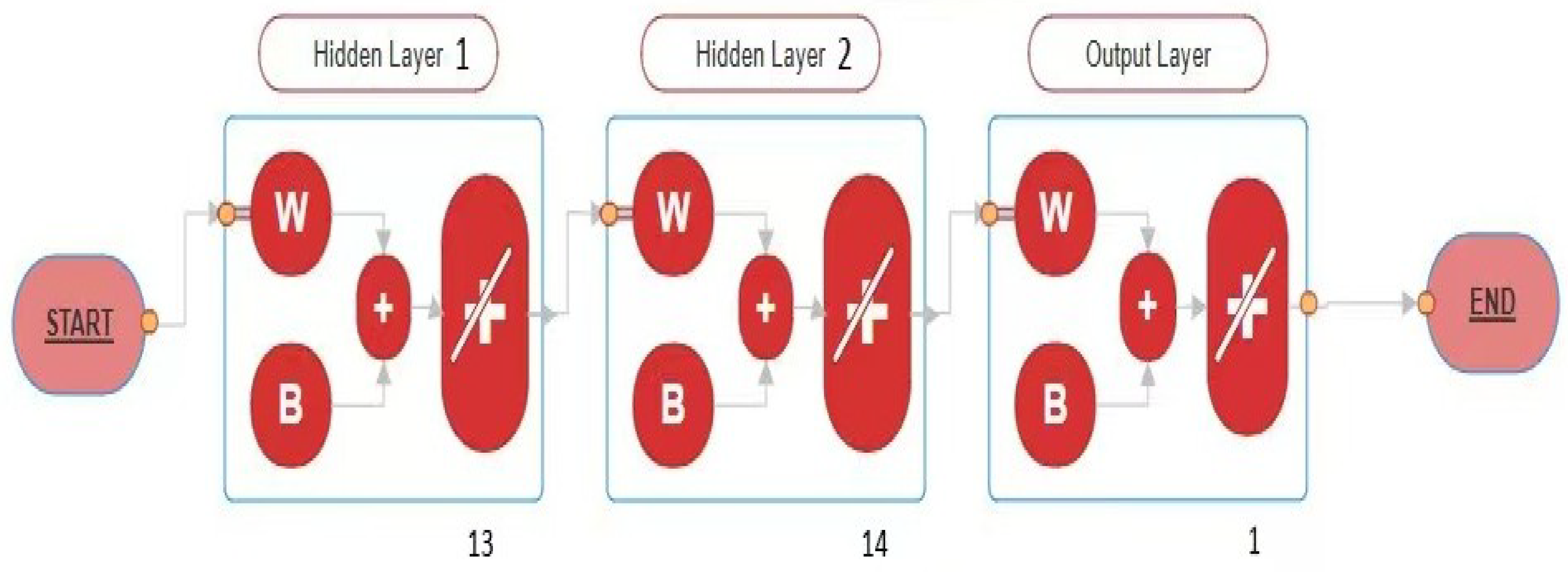
Techniques for machine learning have become crucial for solving everyday issues in the real world. The literature has examined a number of approaches to address these issues. Because of their superior approximation capabilities, ANNs have been used extensively to solve mathematical programming problems. Even with large datasets, ANNs can efficiently estimate nonlinear functions. Three layers make up the structure of a neural network: input, hidden, and output layers. The present work includes a dataset containing the training and testing samples utilized in ANN modeling (along with the input parameters and associated outputs). The dataset was created using the numerical solutions of the governing equations computed in MATLAB. Figure 2 illustrates the net input received by the j-th neuron. The network generates output h from input X. By optimizing the weights and biases of the network nodes, neural network models seek to learn a mapping between the input and output. This research uses an artificial neural network model with an input layer, two hidden layers, and an output layer. The first and second hidden layers contain thirteen and fourteen neurons, respectively. The output layer uses a purelin function, while the two hidden layers use the log-sigmoid activation function, as shown in Figure 3. A physical system has to be mathematically represented before it can be modeled. Mathematical models have many real-world uses and are essential for explaining certain phenomena. Finding the ideal unknown parameters that best describe the system is one of the main goals of these models. Optimization techniques are essential to achieving this objective.
In this context, x i denotes the i-th node in the input layer, a j represents the j-th neuron in the hidden layer, and W 1 j i refers to the weight linking x i to a j . The output of the j-th hidden neuron is given by the following expression:
z j ( x ) = 1 1 + e y j ( x ) .
The expression for the k-th hidden node’s output is as follows:
O k ( x ) = j = 1 m W 2 k j z j + b k .
W 2 k j represents the weight that connects the k-th output layer node to the j-th hidden layer node, and b k denotes the bias term related to the output layer’s k-th node.
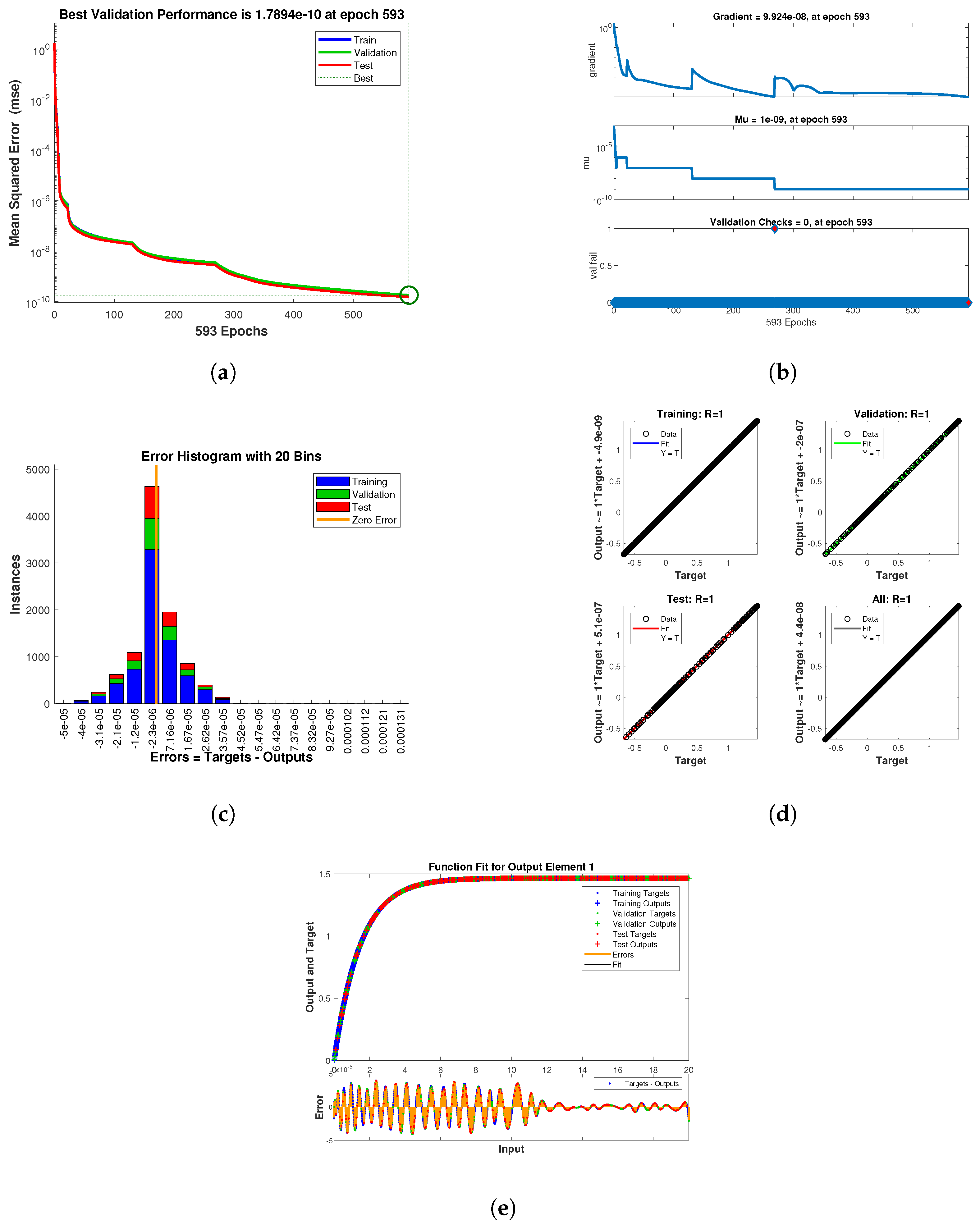
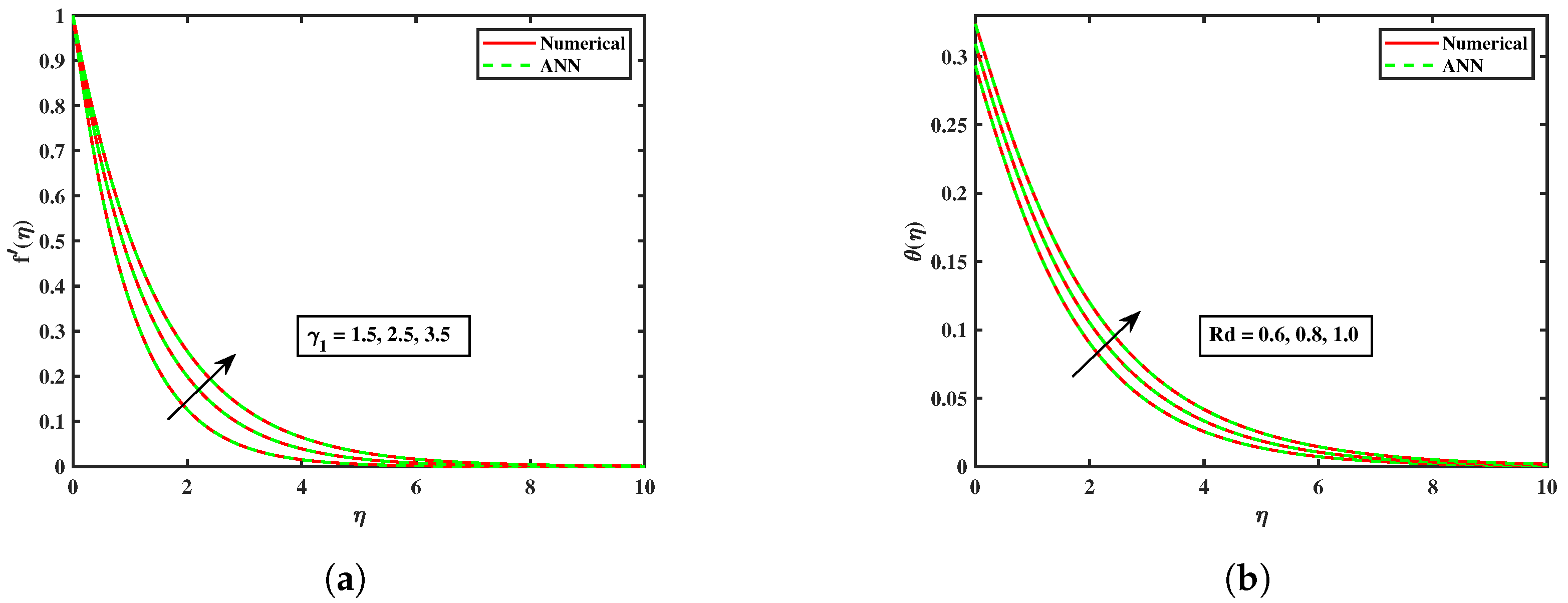
The output neurons of the artificial neural network in this study were utilized to evaluate the mean squared error (MSE), training performance, error distribution, regression analysis, and fitting function across various parameter values of γ 1 and R d , as depicted in Figure 4 and Figure 5. The impact of γ 1 on the velocity equation is shown in Figure 4a–e. Figure 4a shows the best validation performance for the physical parameter γ 1 , which was 1.7894 × 10 10 , obtained at 593 epochs. Figure 4b shows the gradient, M u , and validation. Figure 4c shows an error histogram with 20 bins. Figure 4d shows the regression, which indicates a good fit, while Figure 4e shows the fit function for the input parameter γ 1 . Similarly, the impact of R d on the energy equation is shown in Figure 5a–e. Figure 5a shows the best validation performance for the physical parameter R d , which was 5.8979 × 10 10 , obtained at 346 epochs. Figure 5b shows the gradient, M u , and validation. Figure 5c shows an error histogram with 20 bins. Figure 5d shows the regression, which indicates a good fit, while Figure 5e shows the fit function for the input parameter R d . The ANN predictions with numerical data for the parameters γ 1 and R d are shown in Figure 6. The ANN model’s overall performance shows a good agreement with the numerical data, indicating outstanding accuracy.
The values obtained via computational analysis closely match the outcomes produced by the artificial neural network model. Table 3, Table 4 and Table 5 show the changes in the skin friction coefficient and the Nusselt number in relation to the variables that vary. The acquired numerical data clearly agree with the ANN predictions, indicating strong agreement between the two datasets. As the magnetic parameter M rises, Table 3 shows that the skin friction’s magnitude decreases. Higher levels of M result in a decrease in skin friction because M produces an opposing force that lowers the fluid velocity. Furthermore, the findings shown in Table 3 demonstrate that the Prandtl fluid parameters γ 1 and γ 2 have opposite effects on the skin friction. Similarly, Table 4 and Table 5 show how the Nusselt number is affected by the Prandtl fluid parameters, the radiation parameter, the Biot number, and the magnetic parameter. According to Table 4, as the Prandtl fluid parameters increase, the Nusselt number also increases. Also, the table shows that higher values of the radiation parameter result in an increase in the magnitude of heat transfer. Table 5 indicates that as M increases, the amount of the Nusselt number decreases, but by increasing the Biot number, the Nusselt number shows the opposite behavior. The quantitative results and the artificial neural network model’s outputs closely align, demonstrating the ANN’s capacity to forecast the Nusselt number and the skin friction coefficient.

5. Results and Discussion

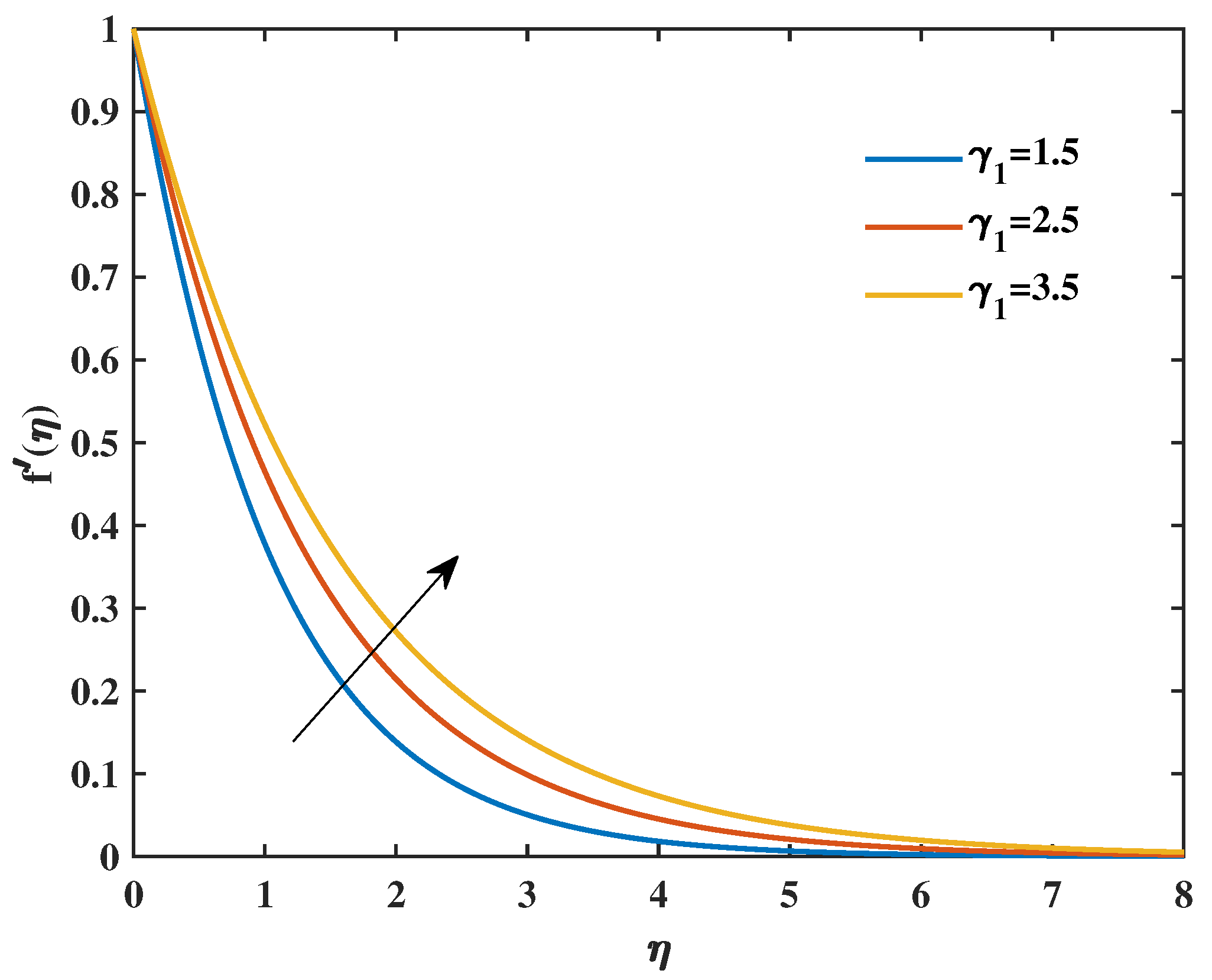
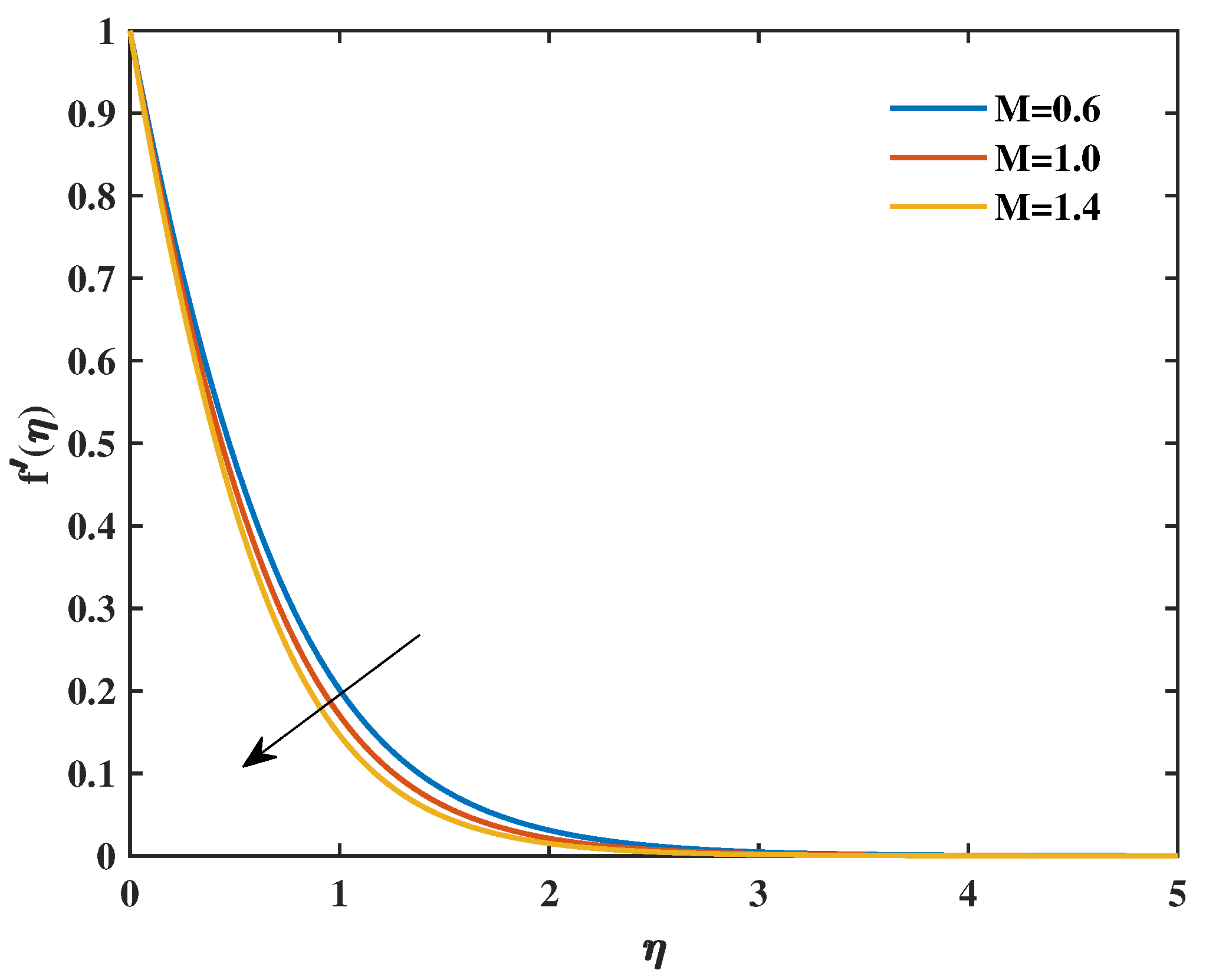
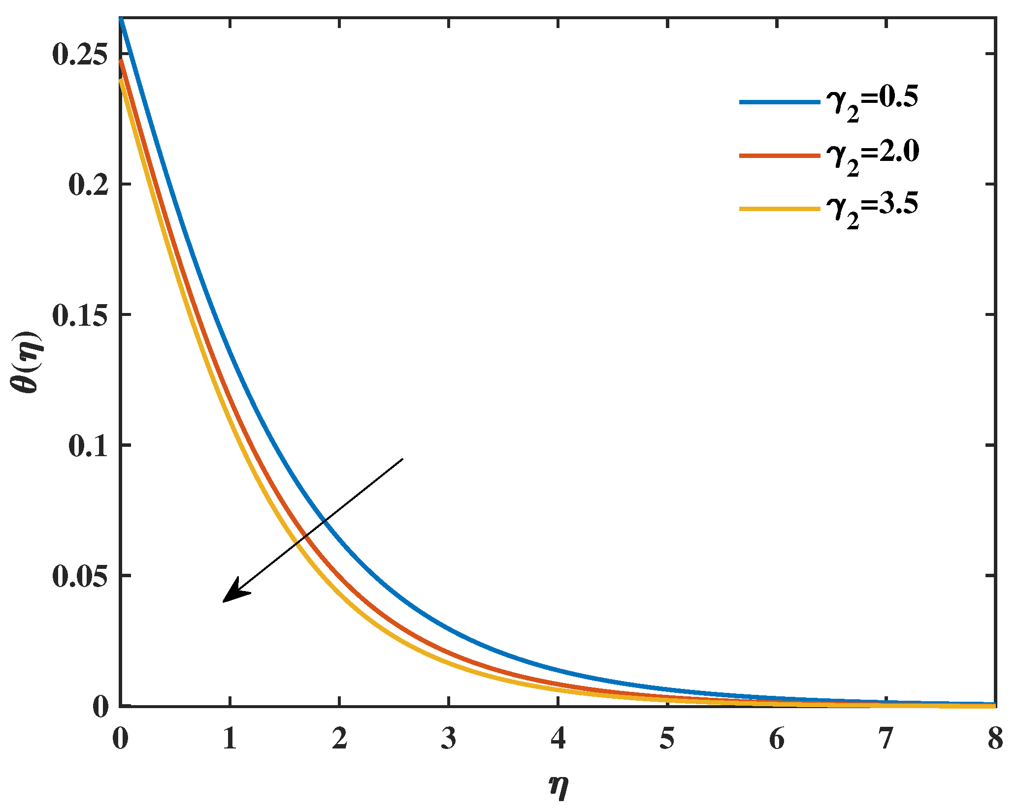
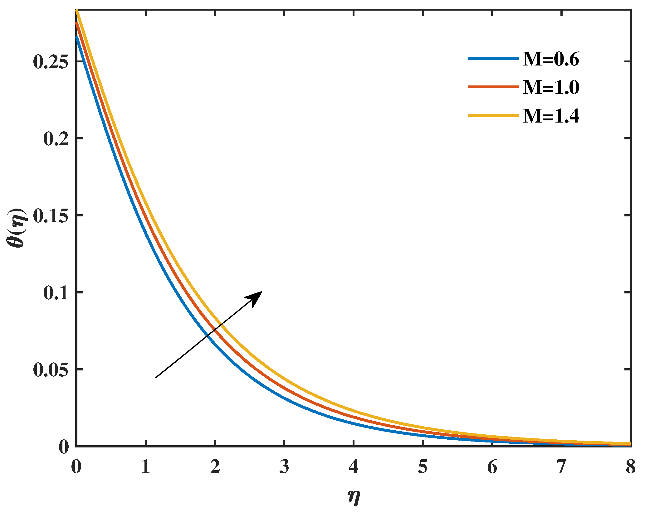
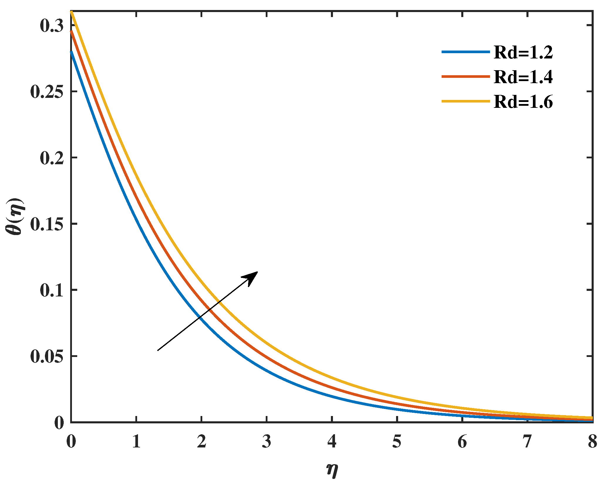
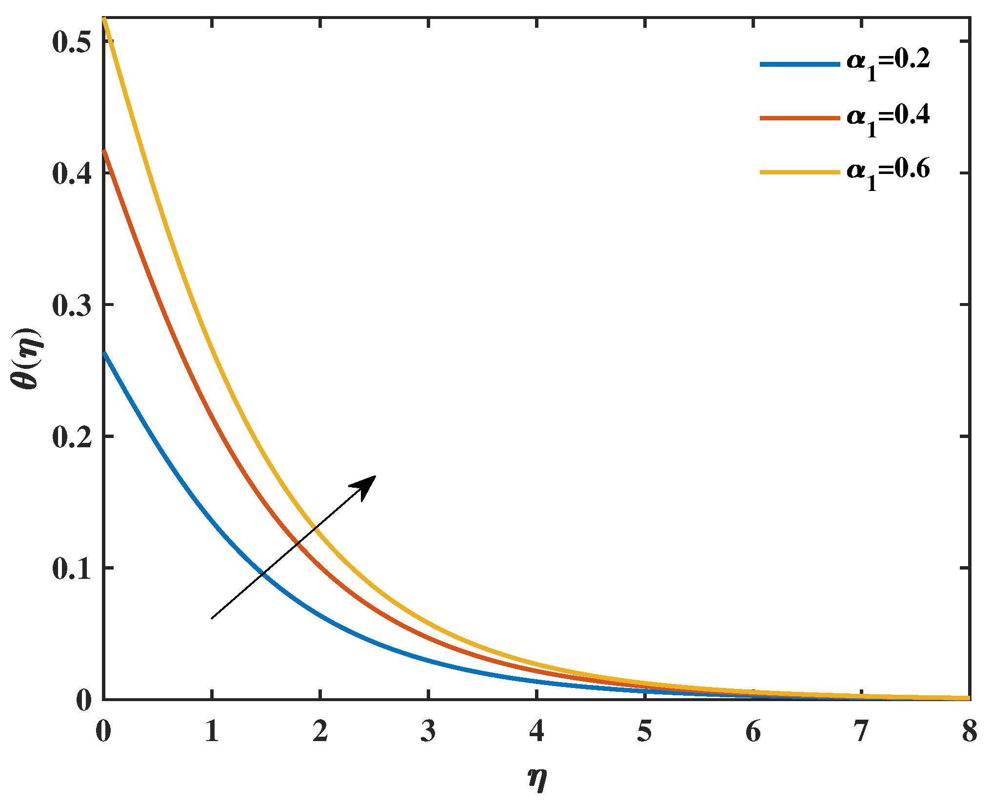
In this work, the flow and heat transfer properties of Prandtl nanofluids under the effect of thermal radiation are compared. The bvp4c shooting technique is used to solve the governing equations while modeling the flow over a stretched sheet. The results are visually represented to allow for a thorough comparison and analysis. The model is numerically computed using specified inputs for parameters such as 0.5 γ 1 3.5 , 0 M 2 , 0.5 γ 2 3.5 , 0 R d 2 , P r = 6.2 , and 0 α 1 1 . Figure 7 and Figure 8 demonstrate how the Prandtl fluid parameters affect the velocity field; higher Prandtl fluid characteristics γ 1 and γ 2 result in increased velocity profiles due to lower effective viscosity, which reduces flow resistance and promotes momentum diffusion. This behavior happens as a result of the fluid’s viscosity decreasing as the Prandtl fluid parameter increases. Consequently, an increase in the Prandtl fluid parameter reduces the fluid’s viscosity, leading to enhanced velocity profiles. However, when the magnetic parameter increases, the velocity decreases, as seen in Figure 9. The electric current created by variations in magnetic flux causes a Lorentz force to be generated by the fluid–magnetic field interaction. It is found that when the strength of the magnetic field increases, the flow of the Prandtl fluid slows down because the Lorentz force opposes the fluid’s motion. As a result, larger magnetic fields result in a reduction in the fluid flow’s boundary layer thickness. Figure 10, Figure 11, Figure 12, Figure 13 and Figure 14 show the effects of the Prandtl fluid parameters, the magnetic parameter, the radiation parameter, and the Biot number on a dimensionless temperature field, respectively. As the ratio of the Prandtl fluid parameters γ 1 and γ 2 increases, the fluid temperature drops, as seen in Figure 10 and Figure 11, respectively. On the other hand, Figure 12 illustrates the opposite pattern for the magnetic parameter M. The reason for this behavior is that a greater M increases the temperature field by strengthening the Lorentz force, which adds more heat. The temperature distribution inside the flow rises as R d increases, as seen in Figure 13. The reason for this is that a greater R d causes more heat energy to enter the flow, which thickens the thermal layer. Furthermore, when the magnetic parameter M is present, the fluid reaches a higher temperature. The influence of the Biot number on the thermal profile is shown in Figure 14. The graphical results have been examined for their practical relevance as well as parameter trends. For instance, the effect of the Biot number α 1 and the magnetic parameter M on surface temperature is important for convective heat transfer augmentation and electromagnetic flow control in cooling systems. These observations provide design recommendations for practical thermal purposes such as energy storage systems, heat exchangers, and electronic cooling. The figure shows that the thermal profile increases as the Biot number increases. The fluid will have a greater temperature close to the surface as the Biot number rises because heat transfer from the surface to the fluid becomes less effective. The fluid’s temperature distribution will change as a result of the thickening of the thermal boundary layer brought on by this rise in temperature near the surface. The rise in temperature profiles with greater radiation parameter R d is attributed to increased radiative heat flow, which thickens the thermal boundary layer. Greater Biot numbers α 1 improve surface-to-fluid heat conduction, leading to greater surface temperatures.

6. Conclusions

This work examined how a stretched horizontal sheet exposed to heat radiation affected the behavior of a Prandtl nanofluid containing copper ( C u ) nanoparticles and water as the base fluid. By applying similarity transformations, the developed nonlinear mathematical model involving multiple parameters was transformed into a system of ODEs. The bvp4c solver in MATLAB was then used to solve these ODEs. The findings were displayed both tabularly and visually. The dataset for the ANN process was created using MATLAB. ANNs are cutting-edge AI tools and were used to improve this model’s solvability. Reliable numerical computing techniques were applied for training, testing, and validating the dataset. This process aimed to provide the intended results, which were subsequently checked for correctness by comparing them with a reference answer. The primary results are summarized as follows, along with a brief description of the major physical elements impacting the flow model:
  • Higher Prandtl fluid parameter values resulted in an increase in the velocity distribution, whereas higher magnetic parameter values produced the opposite effect.
  • Increases in the Biot number, radiation parameter, and magnetic parameter caused the temperature profile to rise.
  • Increases in the Prandtl fluid parameters reduced the temperature distribution.
  • Temperature profiles were enhanced by increasing the values of the magnetic parameter, thermal radiation, and thermal Biot number.
  • As the magnetic parameter and Prandtl fluid parameters increased, the skin friction decreased.
  • As the magnetic parameter increased, the Nusselt number decreased, but increases in the radiation parameters, Prandtl fluid parameters, and Biot number increased it.
  • The bvp4c methodology’s convergence features were demonstrated, and the findings were validated through numerical comparison with the present ANN model, which showed strong agreement in this scenario.

7. Limitations and Future Directions

Table 6 shows a comparison of the current study with Gupta et al. [36] for limited values of parameters. To improve heat transfer efficiency, future studies might investigate hybrid nanofluids, tri-hybrid nanofluids, turbulent flow effects, 3D simulations, and other base fluids. Although this work focuses on Prandtl nanofluid flow based on C u –water, the ANN-integrated solution that is provided may be used for more complex fluid–solid systems, hybrid nanofluids, or other nanoparticle combinations (such as A l 2 O 3 , CNT, or graphene oxide). Future research may potentially incorporate chemically reactive flows or latent heat effects.

Author Contributions

Methodology, S.A.A.S. and M.F.M.; Software, F.S.A. and M.F.M.; Validation, S.A.A.S. and S.B.; Formal analysis, F.S.A. and S.B.; Investigation, M.F.M. and S.B.; Resources, M.F.M.; Data curation, F.S.A.; Writing—original draft, S.A.A.S.; Writing—review and editing, S.A.A.S.; Visualization, S.B.; Supervision, M.F.M.; Project administration, M.F.M.; Funding acquisition, F.S.A. All authors have read and agreed to the published version of the manuscript.

Funding

This work was supported and funded by the Deanship of Scientific Research at Imam Mohammad Ibn Saud Islamic University (IMSIU) under grant number IMSIU-DDRSP2503.

Data Availability Statement

No new data were created or analyzed in this study. Data sharing is not applicable to this article.

Conflicts of Interest

Author Syed Asif Ali Shah was employed by the Jinhua Hangda Beidou Applied Technology Co., Ltd. The remaining authors declare that the research was conducted in the absence of any commercial or financial relationships that could be construed as a potential conflict of interest.

References

  1. Choi, S.U.S.; Eastman, J.A. Enhancing Thermal Conductivity of Fluids with Nanoparticles; No. ANL/MSD/CP-84938; CONF-951135-29; Argonne National Lab. (ANL): Lemont, IL, USA, 1995. [Google Scholar]
  2. Qureshi, M.A. Numerical simulation of heat transfer flow subject to MHD of Williamson nanofluid with thermal radiation. Symmetry 2020, 13, 10. [Google Scholar] [CrossRef]
  3. Raghu, A.; Gajjela, N.; Aruna, J.; Niranjan, H. Significance of modified Fourier heat flux on Maxwell hybrid (Cu-Al2O3/H2O) nanofluid transport past an inclined stretching cylinder. J. Therm. Anal. Calorim. 2024, 149, 12983–13001. [Google Scholar] [CrossRef]
  4. Long, J.; Liu, Z.; Cao, Z.; Wu, J.; Xie, X. Highly efficient pool boiling heat transfer on surfaces with zoned rose-petal-inspired hierarchical structures. Appl. Therm. Eng. 2024, 241, 122330. [Google Scholar] [CrossRef]
  5. Kumar, M.A.; Reddy, Y.D.; Rao, V.S.; Goud, B.S. Thermal radiation impact on MHD heat transfer natural convective nano fluid flow over an impulsively started vertical plate. Case Stud. Therm. Eng. 2021, 24, 100826. [Google Scholar] [CrossRef]
  6. Gajjela, N.; Balakrishnan, A.S.; Garvandha, M.; Niranjan, H.; Raju, A. Impact on induced magnetic field over a second-grade hybrid nanofluid in unsteady thermal systems. Case Stud. Therm. Eng. 2025, 69, 105956. [Google Scholar] [CrossRef]
  7. Kumar, P.; Poonia, H.; Ali, L.; Areekara, S. The numerical simulation of nanoparticle size and thermal radiation with the magnetic field effect based on tangent hyperbolic nanofluid flow. Case Stud. Therm. Eng. 2022, 37, 102247. [Google Scholar] [CrossRef]
  8. Zou, H.; Chen, C.; Zha, M.; Zhou, K.; Xiao, R.; Feng, Y.; Wang, Z. A neural regression model for predicting thermal conductivity of CNT nanofluids with multiple base fluids. J. Therm. Sci. 2021, 30, 1908–1916. [Google Scholar] [CrossRef]
  9. Waqas, H.; Fida, M.; Liu, D.; Manzoor, U.; Alghamdi, M.; Muhammad, T. Heat transport of nanofluid flow through a porous channel with thermal radiation effects. Int. Commun. Heat Mass Transf. 2022, 138, 106376. [Google Scholar] [CrossRef]
  10. Wang, H.; Hou, Y.; He, Y.; Wen, C.; Giron-Palomares, B.; Duan, Y.; Gao, B.; Vavilov, V.P.; Wang, Y. A Physical-constrained decomposition method of infrared thermography: Pseudo restored heat flux approach based on Ensemble Bayesian Variance Tensor Fraction. IEEE Trans. Ind. Inform. 2023, 20, 3413–3424. [Google Scholar] [CrossRef]
  11. Tarakaramu, N.; Satya Narayana, P.V.; Sivakumar, N.; Harish Babu, D.; Bhagya Lakshmi, K. Convective conditions on 3D magnetohydrodynamic (MHD) non-Newtonian nanofluid flow with nonlinear thermal radiation and heat absorption: A numerical analysis. J. Nanofluids 2023, 12, 448–457. [Google Scholar] [CrossRef]
  12. Yan, X.; Feng, Y.; Qiu, L.; Zhang, X. Thermal conductivity and phase change characteristics of hierarchical porous diamond/erythritol composite phase change materials. Energy 2021, 233, 121158. [Google Scholar] [CrossRef]
  13. Basit, M.A.; Imran, M.; Akgül, A.; Hassani, M.K.; Alhushaybari, A. Mathematical analysis of heat and mass transfer efficiency of bioconvective Casson nanofluid flow through conical gap among the rotating surfaces under the influences of thermal radiation and activation energy. Results Phys. 2024, 63, 107863. [Google Scholar] [CrossRef]
  14. Vinutha, K.; Sajjan, K.; Madhukesh, J.K.; Ramesh, G.K. Optimization of RSM and sensitivity analysis in MHD ternary nanofluid flow between parallel plates with quadratic radiation and activation energy. J. Therm. Anal. Calorim. 2024, 149, 1595–1616. [Google Scholar] [CrossRef]
  15. Shoaib, M.; Raja, M.A.Z.; Sabir, M.T.; Islam, S.; Shah, Z.; Kumam, P.; Alrabaiah, H. Numerical investigation for rotating flow of MHD hybrid nanofluid with thermal radiation over a stretching sheet. Sci. Rep. 2020, 10, 18533. [Google Scholar] [CrossRef] [PubMed]
  16. Zainal, N.A.; Nazar, R.; Naganthran, K.; Pop, I. MHD flow and heat transfer of hybrid nanofluid over a permeable moving surface in the presence of thermal radiation. Int. J. Numer. Methods Heat Fluid Flow 2021, 31, 858–879. [Google Scholar] [CrossRef]
  17. Shah, S.A.A.; Ahammad, N.A.; Ali, B.; Guedri, K.; Awan, A.U.; Gamaoun, F.; Tag-ElDin, E.M. Significance of bio-convection, MHD, thermal radiation and activation energy across Prandtl nanofluid flow: A case of stretching cylinder. Int. Commun. Heat Mass Transf. 2022, 137, 106299. [Google Scholar] [CrossRef]
  18. Ramesh, G.K.; Saadeh, R.; Madhukesh, J.K.; Qazza, A.; Khan, U.; Zaib, A.; Abed, A.M. Neural network algorithms of a curved riga sensor in a ternary hybrid nanofluid with chemical reaction and Arrhenius kinetics. J. Radiat. Res. Appl. Sci. 2024, 17, 101078. [Google Scholar] [CrossRef]
  19. Reddy, Y.D.; Goud, B.S. Comprehensive analysis of thermal radiation impact on an unsteady MHD nanofluid flow across an infinite vertical flat plate with ramped temperature with heat consumption. Results Eng. 2023, 17, 100796. [Google Scholar] [CrossRef]
  20. Krishna, M.V.; Kumar, A.V. Chemical reaction, slip effects, and non-linear thermal radiation on unsteady MHD Jeffreys nanofluid flow over a stretching sheet. Case Stud. Therm. Eng. 2024, 55, 104129. [Google Scholar] [CrossRef]
  21. Pourpasha, H.; Farshad, P.; Heris, S.Z. Modeling and optimization the effective parameters of nanofluid heat transfer performance using artificial neural network and genetic algorithm method. Energy Rep. 2021, 7, 8447–8464. [Google Scholar] [CrossRef]
  22. Qiu, L.; Li, Y.; Feng, Y.; Chen, Z.; Zhang, X. Three-dimensional fluid-solid coupling heat transfer simulation based on the multireference frame for a side-blown aluminum annealing furnace. Eng. Appl. Comput. Fluid Mech. 2019, 13, 1036–1048. [Google Scholar] [CrossRef]
  23. Akbar, A.; Ullah, H.; Raja, M.A.Z.; Nisar, K.S.; Islam, S.; Shoaib, M. A design of neural networks to study mhd and heat transfer in two phase model of nano-fluid flow in the presence of thermal radiation. Waves Random Complex Media 2022, 1–24. [Google Scholar] [CrossRef]
  24. Roopa, G.S.; Vishalakshi, C.S.; Madhukesh, J.K.; Ramesh, G.K. Thermal investigation of Tiwari–Das and Xue nanofluid model on space and thermal-dependent heat source/sink over a spinning disk: A numerical study. Numer. Heat Transf. Part Appl. 2025, 1–16. [Google Scholar] [CrossRef]
  25. Rehman, K.U.; Çolak, A.B.; Shatanawi, W. Artificial neural networking (ANN) model for convective heat transfer in thermally magnetized multiple flow regimes with temperature stratification effects. Mathematics 2022, 10, 2394. [Google Scholar] [CrossRef]
  26. Ramesh, G.K.; Shehzad, S.A.; Izadi, M. Falkner–Skan flow of aqueous magnetite–graphene oxide nanoliquid driven by a wedge. Chin. J. Phys. 2022, 77, 733–746. [Google Scholar] [CrossRef]
  27. Hou, Q.; Li, Y.; Singh, V.P.; Sun, Z. Physics-informed neural network for diffusive wave model. J. Hydrol. 2024, 637, 131261. [Google Scholar] [CrossRef]
  28. Nasir, S.; Berrouk, A.S.; Gul, T.; Ali, A. Develop the artificial neural network approach to predict thermal transport analysis of nanofluid inside a porous enclosure. Sci. Rep. 2023, 13, 21039. [Google Scholar] [CrossRef]
  29. Mishra, S.R.; Pattnaik, P.K.; Baithalu, R.; Ratha, P.K.; Panda, S. Predicting heat transfer performance in transient flow of CNT nanomaterials with thermal radiation past a heated spinning sphere using an artificial neural network: A machine learning approach. Partial. Differ. Equ. Appl. Math. 2024, 12, 100936. [Google Scholar] [CrossRef]
  30. Aruna, J.; Niranjan, H. An artificial neural network approach to comparative aspects: A predictive analysis of magnetic dipole on the heat transfer of maxwell hybrid nano coolants flow in an inclined cylinder. Case Stud. Therm. Eng. 2025, 68, 105825. [Google Scholar] [CrossRef]
  31. Awan, A.U.; Qayyum, S.; Nadeem, S.; Ahammad, N.A.; Gepreel, K.A.; Alharthi, M.; Alosaimi, M. Analysis of chemical characteristics of engine-oil-based Prandtl hybrid nanofluid flow. ZAMM-J. Appl. Math. Mech./Z. Angew. Math. Mech. 2024, 104, e202400050. [Google Scholar] [CrossRef]
  32. Shah, S.A.A.; Qayyum, S.; Nadeem, S.; Alzubadi, H.; Ahammad, N.A.; Awan, A.U.; Alroobaea, R. Thermal characterization of Sutterby nanofluid flow under Riga plate: Tiwari and Das model. Mod. Phys. Lett. B 2024, 39, 2450421. [Google Scholar] [CrossRef]
  33. Cao, W.; Animasaun, I.L.; Yook, S.J.; Oladipupo, V.A.; Ji, X. Simulation of the dynamics of colloidal mixture of water with various nanoparticles at different levels of partial slip: Ternary-hybrid nanofluid. Int. Commun. Heat Mass Transf. 2022, 135, 106069. [Google Scholar] [CrossRef]
  34. Cengel, Y.A.; Ghajar, A.J. Heat and Mass Transfer (in SI Units); Mcgraw-Hill Education-Europe: London, UK, 2014. [Google Scholar]
  35. Awan, A.U.; Shah, S.A.A.; Qayyum, S.; Alzubadi, H.; Ahammad, N.A.; Alroobaea, R. Mixed convected synchronization of gyrotactic microorganism flow of an Eyring–Powell nanofluid over a riga plate. ZAMM-J. Appl. Math. Mech./Z. Angew. Math. Mech. 2024, 104, e202301055. [Google Scholar] [CrossRef]
  36. Gupta, D.; Kumar, L.; Anwar Bég, O.; Singh, B. Finite element analysis of MHD flow of micropolar fluid over a shrinking sheet with a convective surface boundary condition. J. Eng. Thermophys. 2018, 27, 202–220. [Google Scholar] [CrossRef]
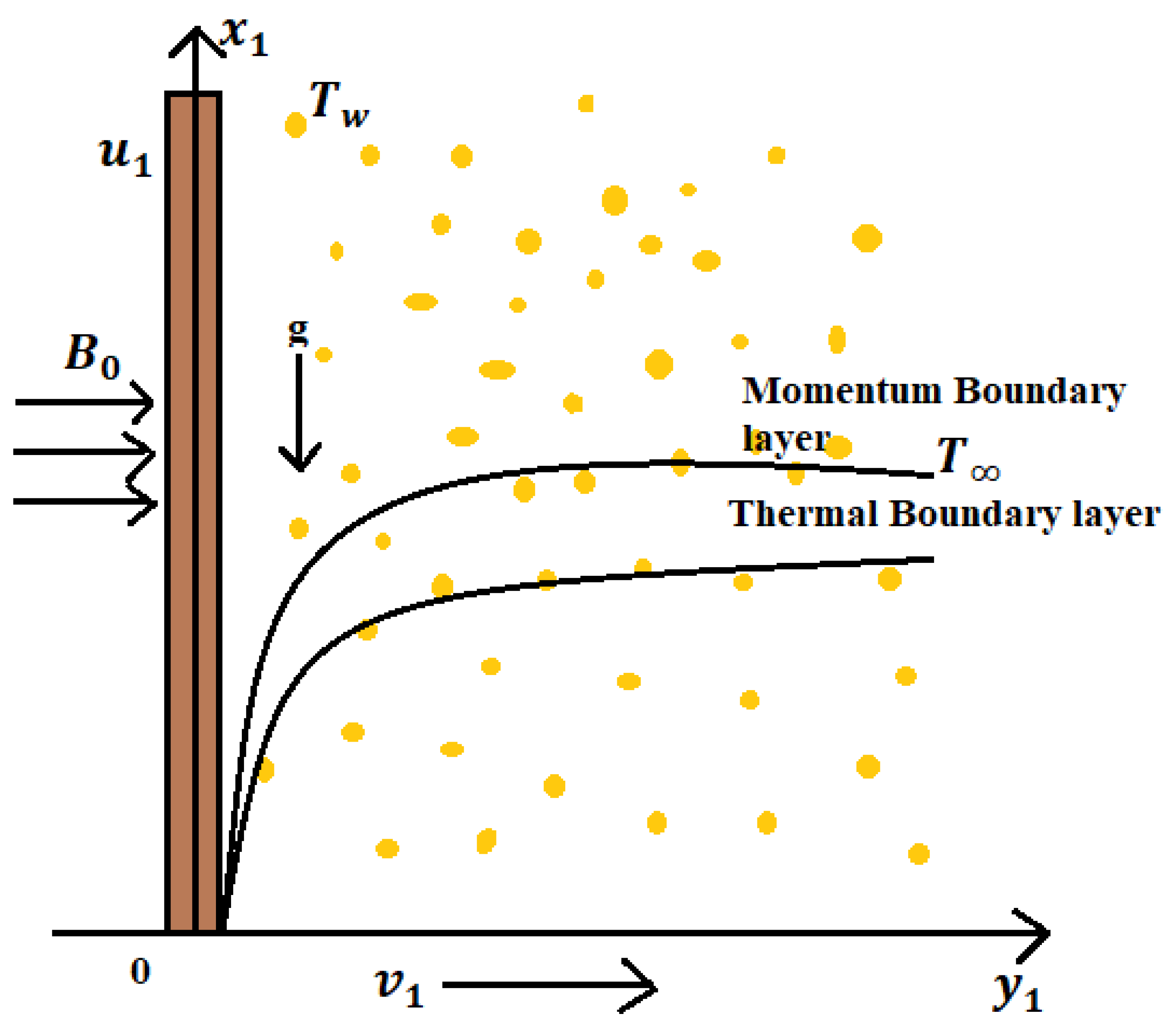
Figure 1. Geometry of the problem.
Symmetry 17 01347 g001
Figure 2. Illustration of the backpropagation of a neural network.
Symmetry 17 01347 g002
Figure 3. ANN model with multiple layers.
Symmetry 17 01347 g003
Figure 4. ANN training for γ 1 : (a) mean squared error; (b) training states; (c) error histogram; (d) regression analysis; (e) function fit.
Symmetry 17 01347 g004
Figure 5. ANN training for R d : (a) mean squared error; (b) training states. (c) error histogram; (d) regression analysis; (e) function fit.
Symmetry 17 01347 g005
Figure 6. Comparison of ANN and bvp4c for different parameters: (a) velocity for γ 1 ; (b) temperature for R d .
Symmetry 17 01347 g006
Figure 7. Influence of γ 1 on f ( η ) .
Symmetry 17 01347 g007
Figure 8. Influence of γ 2 on f ( η ) .
Symmetry 17 01347 g008
Figure 9. Influence of M on f ( η ) .
Symmetry 17 01347 g009
Figure 10. Influence of γ 1 on θ ( η ) .
Symmetry 17 01347 g010
Figure 11. Influence of γ 2 on θ ( η ) .
Symmetry 17 01347 g011
Figure 12. Influence of M on θ ( η ) .
Symmetry 17 01347 g012
Figure 13. Influence of R d on θ ( η ) .
Symmetry 17 01347 g013
Figure 14. Influence of α 1 on θ ( η ) .
Symmetry 17 01347 g014
Table 1. Temperature-dependent characteristics of nanofluids [33].
PropertiesNanofluid
Viscosity μ n f = μ f ( 1 ϕ ) 2.5
Density ρ n f = ρ f ( ( ϕ 1 ) ϕ ( ρ s ρ f ) )
Heat Capacity ( ρ C p ) n f = ( ρ C p ) f ( ( ϕ 1 ) ϕ ( ( ρ C p ) s ( ρ C p ) f ) )
Thermal Conductivity k n f k f = k s + ( m 1 ) k f ( m 1 ) ϕ ( k f k s ) k s + ( m 1 ) k f + ϕ ( k f k s )
Table 2. Physical characteristics of water and C u at a temperature of 293 K [34].
Properties H 2 O Cu
ρ ( Kg · m 3 )997.18933
C p ( J · Kg 1 · K 1 )4179385.0
k ( W · m 1 · K 1 ) 0.6130401.0
σ (Ωm)0.05 5.96 × 10 7
Table 3. Numerical results for the skin friction coefficient with different parameter inputs.
γ 1 γ 2 M Re 0.5 Cf x Re 0.5 Cf x
Bvp4cANNError
0.500.50.5−1.7282−1.75790.0297
0.750.50.5−1.7007−1.70030.0004
1.000.50.5−1.7164−1.70230.0141
1.250.50.5−1.7581−1.75710.001
1.500.50.5−1.8153−1.8170.0017
1.750.50.5−1.8813−1.87920.0021
2.00.50.5−1.9522−1.95280.0006
2.250.50.5−2.0257−2.02840.0027
2.500.50.5−2.1001−2.09860.0015
2.750.50.5−2.1746−2.17170.0029
3.000.50.5−2.2485−2.24690.0016
3.250.50.5−2.3216−2.32050.0011
0.50.500.5−1.7282−1.75790.0297
0.50.750.5−1.9412−1.94080.0004
0.51.000.5−2.1105−2.13680.0263
0.51.250.5−2.2525−2.25170.0008
0.51.500.5−2.3755−2.34190.0336
0.51.750.5−2.4847−2.48480.0003
0.52.000.5−2.5830−2.58360.0006
0.52.250.5−2.6728−2.62720.0456
0.52.500.5−2.7555−2.72020.0353
0.52.750.5−2.8323−2.83550.0032
0.53.000.5−2.9041−2.90560.0015
0.53.250.5−2.9716−2.95730.0143
0.50.50.5−1.8177−1.75790.0598
0.50.50.7−2.0000−1.99980.0002
0.50.50.9−2.1780−2.21140.0334
0.50.51.1−2.3521−2.41750.0654
0.50.51.3−2.5227−2.58470.0620
0.50.51.5−2.6902−2.7040.0138
0.50.51.7−2.8548−2.85290.0019
0.50.51.9−3.0168−3.01720.0004
0.50.52.1−3.1764−3.15450.0219
0.50.52.3−3.3339−3.32350.0104
0.50.52.5−3.4892−3.50060.0114
0.50.52.7−3.6426−3.58790.0547
Table 4. Numerical results for the Nusselt number with different parameter inputs.
γ 1 γ 2 Rd Re 0.5 Nu Re 0.5 Nu
Bvp4cANNError
0.500.51.40.34360.35230.0087
0.750.51.40.34960.35120.0016
1.000.51.40.35360.35870.0051
1.250.51.40.35650.36070.0042
1.500.51.40.35870.35610.0026
1.750.51.40.36040.36160.0012
2.00.51.40.36180.36960.0078
2.250.51.40.36300.36680.0038
2.500.51.40.36390.36280.0011
2.750.51.40.36480.36520.0004
3.000.51.40.36550.36470.0008
3.250.51.40.36610.35940.0067
0.50.501.40.34360.35870.0151
0.50.751.40.34550.35420.0087
0.51.001.40.34700.34780.0008
0.51.251.40.34830.34530.003
0.51.501.40.34930.34640.0029
0.51.751.40.35030.34920.0011
0.52.001.40.35110.35130.0002
0.52.251.40.35180.35120.0006
0.52.501.40.35240.35090.0015
0.52.751.40.35300.35320.0002
0.53.001.40.35360.35320.0029
0.53.251.40.35410.35650.0003
0.50.51.20.37430.36270.0116
0.50.51.40.40370.35870.045
0.50.51.60.43200.40960.0224
0.50.51.80.45910.46610.007
0.50.52.00.48510.50020.0151
0.50.52.20.51020.51690.0067
0.50.52.40.53430.53190.0024
0.50.52.60.55760.55260.005
0.50.52.80.58000.57780.0022
0.50.53.00.60170.60430.0026
0.50.53.20.62260.62850.0059
0.50.53.40.64290.64210.0008
Table 5. Numerical results for the Nusselt number with different parameter inputs.
α 1 M Re 0.5 Nu Re 0.5 Nu
Bvp4cANNError
0.21.50.34360.35870.0151
0.41.50.54380.53520.0086
0.61.50.67480.67550.0007
0.81.50.76730.77110.0038
1.01.50.83600.83280.0032
1.21.50.88910.88190.0072
1.41.50.93140.92920.0022
1.61.50.96580.96770.0019
1.81.50.99440.99360.0008
2.01.51.01851.01520.0033
2.21.51.03911.03830.0008
2.41.51.05691.05740.0005
0.20.50.34360.34160.002
0.20.70.34130.34170.0004
0.20.90.33910.33390.0052
0.21.10.33710.33470.0024
0.21.30.33520.34820.013
0.21.50.33340.35870.0253
0.21.70.33170.34640.0147
0.21.90.33010.32480.0053
0.22.10.32860.32050.0091
0.22.30.32710.32690.0002
0.22.50.32570.32520.0005
0.22.70.32440.32400.0004
Table 6. Skin friction validation for different M with γ 1 = 1 , γ 2 = 0 , R d = 0 , P r = 0 , ϕ = 0 , α 1 .
MGupta et al. [36]Our Results
0.0−1.0000084−0.999306073
1.01.414213561.414213264
5.02.449489742.449489744
10.03.316624793.316627156
50.07.141428437.141424060
100.010.049875610.049871347
500.022.383029322.383023555
1000.031.638584031.638576868
Disclaimer/Publisher’s Note: The statements, opinions and data contained in all publications are solely those of the individual author(s) and contributor(s) and not of MDPI and/or the editor(s). MDPI and/or the editor(s) disclaim responsibility for any injury to people or property resulting from any ideas, methods, instructions or products referred to in the content.