Fusion of k-Means and Local Search Approach: An Improved Angular Bisector Insertion Algorithm for Solving the Traveling Salesman Problem

Abstract

The Angular Bisector Insertion Constructive Heuristic Algorithm (ABIA), though effective for small-scale TSPs, suffers from reduced solution quality and high computational complexity in larger instances due to the degradation of its geometric properties. To address this, two enhanced variants—k-ABIA and k-ABIA-3opt—are proposed. k-ABIA employs k-means clustering to decompose large-scale problems into subgroups, each solved via ABIA, with designed inter-cluster connections to reduce global search cost. k-ABIA-3opt further integrates 3-opt local search and ATSP-specific refinement strategies to avoid local optima. Both algorithms were benchmarked against GA, AACO-LST, and the original ABIA on instances ranging from 100 to 1200 nodes, considering solution quality, stability, runtime, and ATSP performance. k-ABIA-3opt achieved the best overall solution quality, with a total deviation of 28.75%, outperforming AACO-LST (44.86%) and ABIA (144.93%). Meanwhile, k-ABIA, with its O(n²) complexity and low constant overhead, was the fastest, solving 1000-node problems within seconds on standard hardware. Both variants exhibit strong robustness due to minimal stochasticity. For ATSP, k-ABIA-3opt further incorporates directed graph-specific optimization strategies, yielding the best solution quality among all tested algorithms. In summary, k-ABIA-3opt is well-suited for scenarios demanding high-quality solutions within tight time constraints, while k-ABIA provides an efficient option for rapid large-scale TSP solving. Together, they offer scalable and effective solutions for both symmetric and asymmetric TSP instances.

1. Introduction

The symmetric Traveling Salesman Problem (TSP) is a classical NP-hard combinatorial optimization problem that seeks a closed tour with the minimum total distance, given a set of cities and the pairwise distances among them. Mathematically, it is equivalent to finding the minimum Hamiltonian circuit in a weighted complete graph. The history of the problem can be traced back to Euler’s study of the knight’s tour in the 18th century, while its modern formal definition was clearly presented by Karl Menger in the 1930s. The problem gained significant attention in the 1950s when Dantzig and Johnson successfully solved a 49-city instance using cutting plane methods [1,2]. In 1972, Richard M. Karp proved that the Hamiltonian circuit problem is NP-complete, indirectly establishing the NP-completeness of the TSP and providing a theoretical basis for its computational complexity [1]. As the number of cities increases, the search space grows exponentially. For example, the number of possible tours for 30 cities reaches the order of 1032, with the possibilities for symmetric and asymmetric TSP being n!/2 and n!, respectively [3]. The asymmetric TSP (ATSP) refers to the case when a weighted complete graph is converted into a weighted complete directed graph, where the cost of arc (i, j) is not equal to that of (j, i). This asymmetry prevents ATSP from being simplified to the TSP and necessitates an explicit treatment of directional constraints [4]. The TSP also serves as a mathematical foundation for a wide range of real-world applications, including circuit board drilling, logistics routing, warehouse robotics, and various combinatorial optimization problems involving cost minimization.

Current methods for solving the TSP fall into two categories: exact algorithms and heuristic algorithms. Exact algorithms, which guarantee finding the optimal solution, include methods such as branch-and-bound, the Dantzig–Fulkerson–Johnson (DFJ) integer programming model, and dynamic programming. The core idea of the branch-and-bound method is to recursively partition the search space (branching) and eliminate non-promising subsets (bounding) to gradually approach the optimal solution [5]. The DFJ integer programming model ensures that the TSP forms a single tour by adding appropriate constraints, although the number of these constraints grows on the order of $O(2^n)$ [6]. The Held–Karp algorithm, a dynamic programming approach, has a time complexity of $O(n^2·2^n)$, rendering it practical only for up to 30 cities due to substantial memory requirements [7]. While exact algorithms guarantee optimality, they become prohibitively difficult to solve for large-scale instances owing to the enormous computational resources required [8,9]. Consequently, exact algorithms are generally suited to small-scale problems or applications requiring very high accuracy—such as last-mile drone delivery [10] and path planning in integrated circuit lithography.

When exact algorithms encounter computational bottlenecks, heuristic algorithms can quickly obtain approximate solutions by mining problem-specific features and applying intelligent search strategies. Heuristic methods can be further divided into metaheuristic algorithms, deep learning-based solvers, and constructive heuristics. Metaheuristics, which remain a hot research topic, simulate natural phenomena or collective intelligence to perform guided random searches in the solution space. Notable examples include the Migrating Birds Optimization (MBO) algorithm, which mimics the cooperative mechanisms of migrating birds (e.g., formation flying and information sharing) [11]; Genetic Algorithms that simulate natural selection, crossover, and mutation processes [12]; the relatively novel Grey Wolf Optimization, inspired by the social behaviors of gray wolves [13]; and the Discrete Artificial Bee Colony (DABC) algorithm, which models the foraging behavior of bees and integrates domain-specific operators for optimization [14]. Among swarm intelligence methods, the Ant Colony Optimization algorithm is particularly popular, simulating the pheromone-based foraging behavior of ants to find better paths [15]. Particle swarm optimization, inspired by the synchronized speed adjustments observed in bird flocks, achieves rapid convergence in continuous spaces [16]. A more recent development is the Discrete Tree Seed Algorithm (DTSA), which mimics the natural process of tree propagation—including seed generation, dispersal, and survival of the fittest—to accommodate the characteristics of permutation-based optimization problems [17]. In recent years, parallel optimization strategies have been widely adopted in swarm intelligence algorithms. For example, the Parallel Binary Cat Swarm Optimization (PBCSO) algorithm divides the population into multiple subgroups that evolve independently and periodically exchange information through communication mechanisms to enhance global search capabilities [18]. In addition, the Discrete Symbiotic Organisms Search (DSOS) algorithm, which fuses gene transfer and path crossover elimination strategies, facilitates information exchange among multiple groups of symbiotic organisms and effectively mitigates the tendency of traditional discrete symbiotic algorithms to get trapped in local optima and exhibit insufficient convergence when solving the TSP [19].

With the rise in deep learning in recent years, end-to-end training methods can directly learn path construction rules from TSP instances, thereby overcoming the reliance on the domain knowledge characteristic of traditional algorithms. For example, a method based on the Transformer architecture uses reinforcement learning for training without relying on pre-existing TSP solutions [20]. Another study developed a deep learning framework that employs deep convolutional networks to extract features from TSP instances, integrating data augmentation techniques to handle complex cases [21]. Moreover, Q-learning has been applied to optimize TSP formulations in multi-robot formation tasks [22]. In addition, deep learning models can be combined with heuristic algorithms—such as hybrid genetic algorithms and multi-agent reinforcement learning algorithms—to solve the TSP [23]. By merging metaheuristics and deep learning, researchers primarily target medium-to-large TSP instances, achieving faster solution speeds with smaller deviations. These methods find broad applications, including optimizing meal-preparation sequences for restaurant chefs [24], handling large-scale pharmaceutical and fresh produce deliveries [25], implementing the Multi-Traveling Salesman Problem (M-TSP) for multi-vehicle cooperative distribution [26], and planning municipal garbage truck routes in conjunction with genetic algorithms to reduce travel distance [27].

However, certain scenarios impose strict requirements on both response time and solution stability, making traditional metaheuristics or deep learning approaches less directly applicable. Examples include the following:

• Food delivery systems require real-time route updates (within 1 s per new order) under dynamic order influx. Traditional metaheuristics suffer from prolonged iteration times (minute-level) and potential solution instability during dynamic adjustments.
• Earthquake rescue drones necessitate rapid coverage path planning in communication-constrained environments.
• Network base station repairs demand immediate multi-site maintenance route generation to prevent service disruptions.
• Robotic formation tasks require both rapid response and high stability for coordinated maneuvers.

In such contexts, constructive heuristic algorithms demonstrate distinct advantages due to their inherent properties:

(1)

Single-pass solution construction: Feasible solutions are generated directly via deterministic or semi-deterministic rules, bypassing iterative optimization and enabling millisecond-level computation.

(2)

Rule-driven stability: Deterministic construction rules ensure consistent outputs, mitigating solution volatility.

(3)

Domain knowledge integration: Heuristic rules explicitly embed domain-specific constraints (e.g., traffic regulations, physical limitations) with minimal parameter tuning and straightforward implementation.

Prominent constructive heuristics include the nearest-neighbor method [28], farthest insertion [29], convex hull algorithm [30], and the recently proposed Angular Bisector Insertion Algorithm (ABIA) [31].

The Angular Bisector Insertion Algorithm (ABIA) leverages the spatial distribution characteristics of point sets to construct angular bisectors that partition the set into left and right subsets. It then incrementally inserts the points from these subsets into a tour according to predefined insertion rules. As a constructive heuristic algorithm based on geometric principles, ABIA demonstrates strong performance in small-scale Traveling Salesman Problems (TSPs), characterized by solution stability, high computational efficiency (at the millisecond level), and high solution quality. However, when applied to large-scale or high-complexity asymmetric TSPs (ATSPs), ABIA suffers from limitations such as reduced solution quality and increased computational complexity. The core challenge lies in effectively reducing the overall problem complexity. To address this, a “Divide-Connect-Optimize” three-level collaborative strategy has emerged as a key approach to enhancing ABIA’s performance. This divide–solve–connect framework was first proposed by Croes (1958) and has since become a classical model supporting both symmetric and asymmetric TSPs in automated solution processes [32]. Recent studies have increasingly focused on integrating clustering-based pre-segmentation techniques—aimed at reducing subproblem sizes—with metaheuristic optimization methods that improve solution quality. One notable example is the hybrid strategy combining k-means clustering and the Ant Colony Optimization algorithm [33].

In this work, the k-means clustering algorithm [34] is employed to partition the point set, with each resulting small-scale TSP subproblem solved using the ABIA. Subsequently, inter-cluster connection rules are constructed to link multiple TSP tours. To accommodate the structural differences between TSP and ATSP, distinct inter-cluster connection strategies are designed accordingly. After the inter-cluster tour is formed, a post-processing phase is applied, incorporating the 3-opt algorithm [35] along with a set of custom-designed path refinement rules, to mitigate the risk of convergence to local optima.

This framework yields two improved variants of ABIA: one that integrates k-means clustering and 3-opt optimization (termed k-ABIA-3opt), which focuses on enhancing solution quality; and another that omits the 3-opt refinement step (termed k-ABIA) to emphasize computational efficiency. Both variants are applicable to TSP instances of varying scales and application requirements. Given node coordinates and the pairwise distances (or weights) between nodes, the algorithm can generate a directed or undirected tour that minimizes the total travel cost or distance. Beyond solving TSP and ATSP, the core design philosophy underlying the proposed methods—namely, complexity reduction through clustering and solution refinement via local heuristics—may hold potential for broader applications such as feature selection in high-dimensional data analysis [36]. For instance, in problems like sparse linear discriminant analysis for image classification, where selecting representative subsets from large feature spaces is essential, similar clustering and path construction strategies could be adapted to identify optimal feature combinations. While the current study remains focused on combinatorial routing problems, this direction suggests promising avenues for future cross-domain extensions.

The structure of this paper is organized as follows:

Section 2 introduces the related research, including the Angular Bisector Insertion Algorithm, k-means clustering, and 3-opt optimization.

Section 3 details the proposed improved Angular Bisector Insertion Algorithm that fuses k-means and 3-opt.

Section 4 provide an analysis of the characteristics and time complexity of the improved algorithm.

Section 5 presents comparative experiments using TSPLIB standard datasets, contrasting the performance of the proposed algorithm with the traditional ABIA and a genetic algorithm.

Section 6 concludes the study and discusses future research directions.

2. Related Research

2.1. Mathematical Models of TSP and ATSP

The Traveling Salesman Problem (TSP) is defined on a complete weighted undirected graph G = (V, E), where V = {1,2,…,n} represents the set of n cities (or nodes) and E is the set of edges connecting each pair of cities. Each edge $\left(i,j\right)\in E$ is associated with a non-negative distance (or cost) d_ij.

The objective is to determine a Hamiltonian cycle that visits each city exactly once and returns to the starting city while minimizing the total travel cost. The classical integer linear programming (ILP) formulation of the symmetric TSP is

$$\min {\displaystyle \sum _{i=1}^n{\displaystyle \sum _{j=1}^n{d}_{ij}}}{x}_{ij}$$

(1)

subject to

$${\displaystyle \sum _{j=1}^n{x}_{ij}}=1,\forall i\in V,$$

(2)

$${\displaystyle \sum _{i=1}^n{x}_{ij}}=1,\forall j\in V,$$

(3)

$$x_{ij}\in \left\{0,1\right\}, \forall i,j\in V,i\ne j,$$

(4)

where x_ij = 1 if the tour travels directly from city i to city j, and x_ij = 0 otherwise. To prevent the formation of disconnected subtours, additional subtour elimination constraints, such as the Dantzig–Fulkerson–Johnson (DFJ) constraints, are required:

$${\displaystyle \sum _{i\in S}{\displaystyle \sum _{j\in S}{x}_{ij}}}\le \left|S\right|-1, \forall S\subset V,2\le \left|S\right|\le n-1.$$

(5)

Here, S denotes any non-empty proper subset of nodes in V, and $\left|S\right|$ is the cardinality of this subset. These constraints ensure that no feasible solution can form a smaller closed loop within the subset S without visiting the remaining nodes, thereby guaranteeing a single Hamiltonian cycle. The Asymmetric Traveling Salesman Problem (ATSP) is a more general form of the TSP in which the travel cost is direction-dependent, i.e., $d_{ij}\ne d_{ji}$ in general.

2.2. Angular Bisector Insertion Algorithm

The ABIA is a constructive heuristic whose core idea is to “open up” the tour by exploiting the properties of the angular bisector, first constructing an outer Hamiltonian circuit and then progressively inserting the interior points. The algorithm consists of the following three steps:

• Construction of the Initial Tour
  Given a set of points V = {a, b, c, d, e, f, g, o}, let d_ij denote the distance between point i and point j, and let e_ij represent the edge connecting these two points. Define d(i, L) as the perpendicular distance from point i to the angle bisector L, with the reference point denoted as o. The procedure is as follows:

  (1)

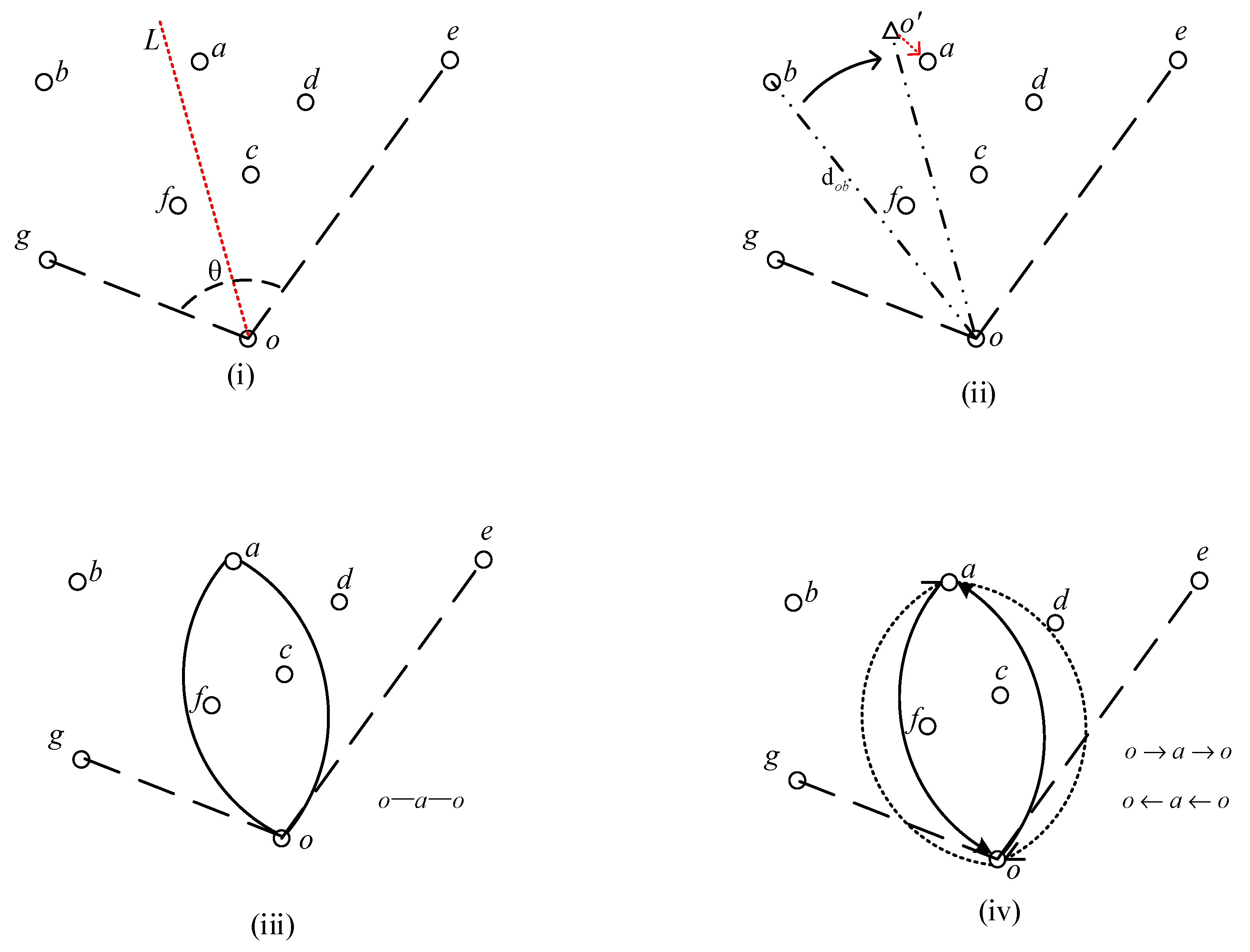
  Identify the leftmost and rightmost points in the set to construct a sector region, as illustrated in Figure 1i, where the sector $\angle \theta$ is defined by og and oe.

  (2)

  Compute the angle bisector L of the sector.

  (3)

  Determine the maximum distance from o to any other point in the set, denoted as $d_{ob}=\max (d_{oi}|i\in V)$ in Figure 1ii.

  On the angle bisector L, mark a new point o’ such that the distance from o to o’ equals d_ob, and identify point $\min (d_{o^{\prime }j}|j\in V)$. Connect this point (e.g., point a as shown in Figure 1ii) to the origin o, forming the initial loop as depicted in Figure 1iii. For the ATSP, two directed loops are created as shown in Figure 1iv.

2.

Insertion Node Selection

Let the initial loop be represented by the point set S = {o,a}. The next insertion point j is selected from the remaining nodes in $V\backslash S$, and it must satisfy the condition: $\max \left(d\left(m,L\right)|m\in V\backslash S\right)$.

3.

Node Insertion into the Loop

Traverse all edges in the current tour to identify eligible insertion positions. When the condition

$$\min (d_{uj}+d_{jv}-d_{uv}|u,v\in S)$$

(6)

is satisfied, insert node j between points u and v. And steps 1 and 2 are repeated until all points are inserted into the loop, forming the final loop.

In the case of the ATSP, the node j must be inserted into the loop in both clockwise and counterclockwise directions:

The insertion cost in the counterclockwise direction is as shown in Equation (6).

The insertion cost in the clockwise direction is

$$\min (d_{vj}+d_{ju}-d_{vu}|u,v\in S)$$

(7)

Steps 2 and 3 are repeated until all nodes are inserted. After all nodes are inserted, the complete clockwise and counterclockwise loops are compared, and the one with the minimum total cost is selected as the final optimal loop.

2.3. k-Means Clustering Algorithm

The k-means algorithm is a classical clustering method that iteratively optimizes the partitioning of data into a specified number of clusters (k), aiming to maximize the similarity within clusters and maximize the dissimilarity between clusters [35]. The main steps of the algorithm are as follows:

• Initialization: Randomly select k sample points as initial centroids, with each centroid representing the core location of a cluster.
• Sample Assignment: Compute the distance (typically Euclidean distance) between all samples and the centroids, assigning each sample to the cluster of the nearest centroid, thus forming an initial clustering.
• Centroid Update: Recalculate the centroid of each cluster (i.e., the average x and y coordinates of the points within the cluster), which serves as the new center point.
• Iterative Optimization: Repeat steps 2 and 3 until the centroids no longer change, sample assignments stabilize, or the preset number of iterations is reached, at which point the algorithm terminates.

The core objective of the algorithm is to minimize the sum of squared errors within clusters (SSE):

$$SSE={\displaystyle \sum _{i=1}^{\mathrm{k}}{\displaystyle \sum _{x\in C_i}{‖x-{\mu }_i‖}^2}}$$

(8)

Here, ${\mu }_i$ represents the centroid of the i-th cluster, and $C_i$ denotes the set of sample points belonging to that cluster.

2.4. The 3-Opt Algorithm

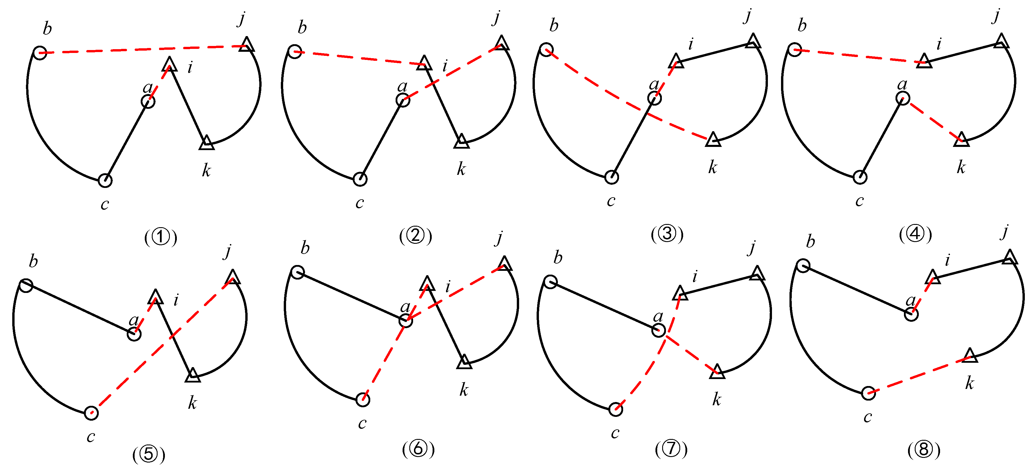
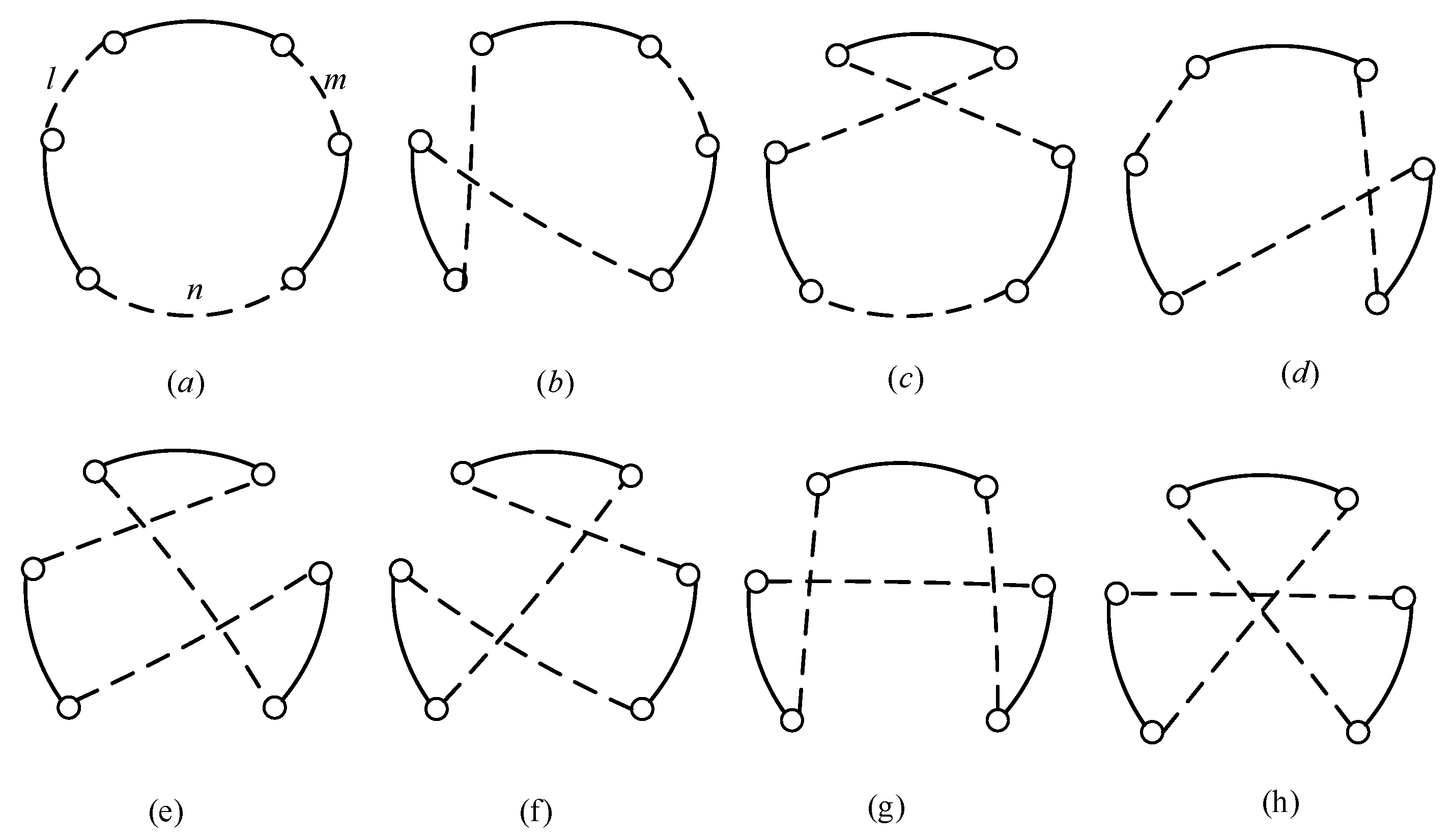
The 3-opt algorithm is a classic local search optimization method primarily used to solve the Traveling Salesman Problem (TSP). It is a form of the k-opt heuristic algorithm, which improves the solution quality by removing three edges from the current path and reconnecting the disconnected parts in different ways [36]. As shown in Figure 2, there are eight distinct ways to reconnect the broken edges l, m, and n [37], forming a new loop (the dashed lines represent the reconnected paths).

The specific implementation steps of the 3-opt algorithm are as follows:

(a)

Randomly select three nodes: Choose i, j, and k using a nearest-neighbor approach.

(b)

Compute all possible reconnection methods: Reconstruct the path using the eight connection methods shown in Figure 2 and verify whether each reconnection reduces the total path length.

(c)

Select the optimal improvement: Retain the best combination that shortens the path length and update the current solution.

(d)

If no further optimization is possible or the stopping condition (e.g., a set number of iterations) is met, output the current solution.

3. Algorithm Proposal

To address the issue of poor solution quality when solving large-scale TSPs using the ABIA, this paper introduces the k-means algorithm to divide the large TSP into multiple smaller TSP subproblems. For each smaller TSP, the ABIA’s strengths—such as excellent solution quality for small-scale problems, high stability, and fast computation speed—are leveraged for solving. Additionally, inter-cluster connection rules are established to effectively link the paths between multiple clusters. Furthermore, due to the insertion characteristics of the ABIA, which may lead to local optima, this paper further incorporates the 3-opt algorithm for optimization, thus improving solution quality and global search capability. Based on this, an improved Angle Bisector Insertion Algorithm, integrating k-means and 3-opt, is proposed to further enhance the TSP solving performance. The algorithm steps are as follows:

• Use the k-means algorithm to cluster the TSP point set. Let the number of points in the TSP be n, and the total set of TSP points is

$$V=\{v_1,v_2,\dots ,v_n\}$$

(9)

Divide the point set into k clusters:

$$C=\{C_1,C_2,\dots ,C_k\}, \mathrm{where} k=round(n/100)$$

(10)

Each cluster satisfies

$${\displaystyle \underset{i=1}{\overset{k}{\cup }}{C}_i}=V, C_i\cap C_j=\varnothing (i\ne j)$$

(11)

Since the ABIA demonstrates superior solution quality and computation speed for up to 100 points, the number of clusters $k=round(n/100)$ is set to appropriately partition the problem size.

2.

For each cluster $C_i$, apply the ABIA to solve the TSP path (parallel processing can be employed to improve efficiency):

$$T_i=\mathrm{ABIA}(C_i), i=1,2,\dots ,k$$

(12)

3.

To connect all clusters, a nearest-point connection search strategy between clusters is defined to identify the optimal connection scheme between cluster C_i and cluster C_j.

Within clusters C_i and C_j, the closest pair of points is identified:

$$(p_i,p_j)=\arg \underset{(p_i\in C_i,p_j\in C_j)}{\min }d(p_i,p_j)$$

(13)

Suppose the closest pair of points is $\left(a,i\right)$, where a is a point in cluster $C_i$, $i$ is a point in cluster j, b and c are the adjacent points before and after a, and j and k are the adjacent points before and after $i$. Based on different edge disconnection strategies, the following eight connection methods are designed (other points in the loop are omitted), as shown in Figure 3:

①$b\to j,a\to i$②$b\to i,a\to j$③$b\to k,a\to i$④$b\to i,a\to k$⑤$a\to i,c\to j$⑥$c\to i,a\to j$⑦$c\to i,a\to k$⑧$a\to i,c\to k$; there are eight connection methods in total. The distance variations are computed, and the scheme with the shortest total distance is selected to optimize the overall inter-cluster connection. This strategy ensures that the inter-cluster connections are efficient and adhere to the optimal path principle, thereby improving the global solution quality.

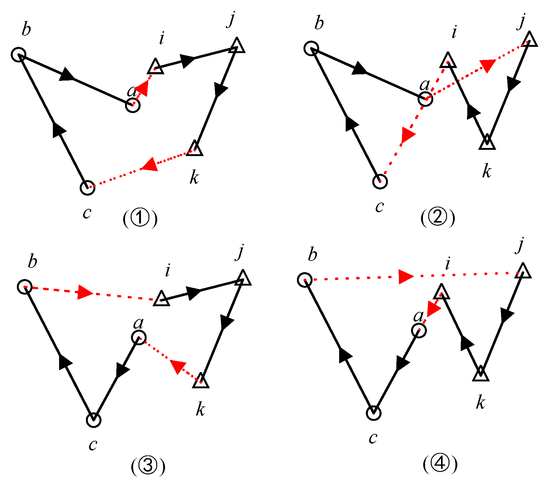
In the ATSP, since the loops generated by the ABIA are directional, the designed connection scheme must consider directionality constraints. Cluster $C_i$ can disconnect either the ac or ba edge and can also disconnect either the ij or ki edge. By disconnecting one edge from each pair, a connection method is determined. Therefore, there are a total of four connection methods, as shown in Figure 4: ①$a\to i,k\to c$②$i\to c,a\to j$③$b\to i,k\to a$④$b\to j,i\to a$.

4.

After merging the clusters to form a complete loop, direct connections between multiple clusters are prone to getting stuck in local optima, affecting the final path quality. Therefore, the 3-opt algorithm is introduced to optimize the path, thereby improving the overall solution quality. However, the traditional 3-opt algorithm is primarily suited for the TSP and needs to be appropriately adjusted for the ATSP to fit the problem characteristics.

Inspired by the 3-opt optimization approach, the complete TSP loop is divided into four continuous path segments using three splitting points (in conjunction with the starting point), as shown in Figure 5. Here, let o be the starting point of the loop, and i, j, and k represent the three key splitting points. The loop can then be divided into the following four path segments.

seq1: The path from the starting point o to i;

seq2: The path from i + 1 to j;

seq3: The path from j + 1 to k;

seq4: The path from k + 1 to the endpoint z.

During the optimization process, to ensure the consistency of the loop’s direction, only the exchange of different path segments is allowed, without changing the direction of node visits. Based on this, three path exchange methods are designed to optimize the overall path length:

(a)

Exchange seq1 with seq2, adjusting the path structure between the starting point and the first partition point.

(b)

Exchange seq2 with seq3, optimizing the path connection in the middle segment.

(c)

Exchange seq3 with seq4, adjusting the connection method of the terminal path.

After each exchange, the length of the optimized path is calculated. If the new path length is shorter than the original path, the exchange operation is accepted, continuously iterating to optimize the overall loop structure. This improvement strategy further enhances the final solution quality, resulting in better paths after cluster merging, leading to the final solution.

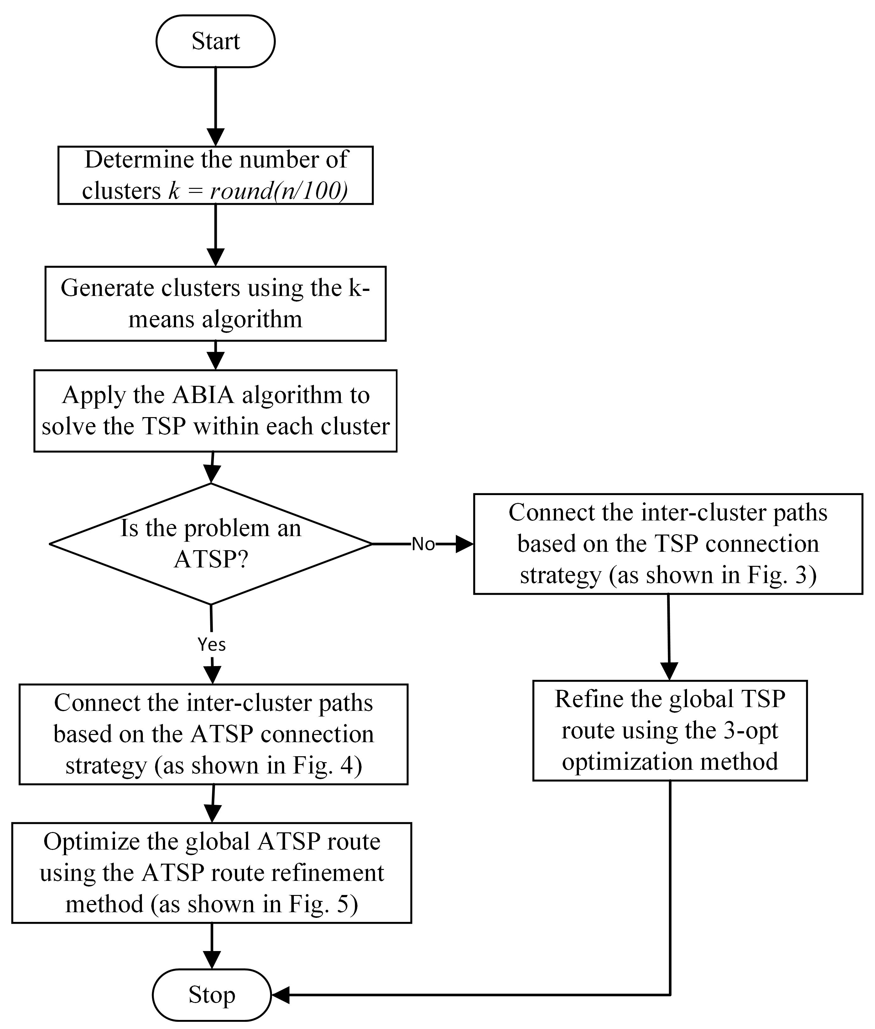
In summary, the improved Angular Bisector Insertion Algorithm (ABIA), which integrates K-means clustering and 3-opt optimization, consists of four main steps, as detailed in the pseudocode in Algorithm 1 and illustrated by the flowchart in Figure 6. It is worth noting that Step 4 (Path Optimization) is an optional step; omitting it can significantly reduce the computational time, especially for large-scale problem instances.

Algorithm 1 Improved Angular Bisector Algorithm Combining K-means and 3-opt (TSP Point Set V, Distance Matrix D)
1	Step 1: Clustering Division
2	Clusters ← KMeans(V, k)  //$k=round(n/100)$, n represents the number of point groups.
3	Step 2: Calculate the optimal path within the cluster.
4	for each Cluster in Clusters do
5	LocalRoute[Cluster] ← ABIA(Cluster, D)  // Optimize the intra-cluster path using the ABIA.
6	end for
7	Step 3: Connect the inter-cluster path.
8	if   ProblemType == TSP then
9	GlobalRoute ← ConnectClusters_TSP(LocalRoute, D)  // The 8 connection methods used (Figure 3).
10	else if ProblemType == ATSP then
11	GlobalRoute ← ConnectClusters_ATSP(LocalRoute, D)  // The 4 connection methods used (Figure 4).
12	end if
13	Step 4: Path optimization.
14	if    ProblemType == TSP then
15	GlobalRoute ← 3OptOptimization(GlobalRoute, D)  // Path optimization using 3-opt (Figure 2).
16	else if    ProblemType == ATSP then
17	GlobalRoute ← PathExchangeOptimization(GlobalRoute, D)  //Path exchange optimization (Figure 5).
18	end if
19	Return GlobalRoute

4. Algorithm Characteristics and Complexity Analysis

The time complexity of this algorithm is mainly composed of four parts: k-means clustering, angle bisector algorithm, inter-cluster connection optimization, and 3-opt local optimization. The following is a detailed analysis of each module:

• k-means Clustering Phase
  The time complexity of k-means is $O\left(knt\right)$, where n is the total number of points, k is the number of clusters, and t is the number of iterations [37]. In this work, the number of clusters k is adaptively set as $k\approx n/100$ to constrain the cluster size to approximately 100 points. Under this assumption and considering that the number of K-means iterations t remains constant, the time complexity of the clustering phase simplifies to $O\left(n^2\right)$.
• Angle Bisector Algorithm
  The time complexity for a single computation of the angle bisector algorithm is

  $$O\left(3n^2+{\displaystyle \frac{2n^3-8n^2+8n}{2}}\right)$$

  (14)
  Here, n represents the number of points [30]. The time complexity of a single execution of the Angle Bisector Insertion Algorithm (ABIA) can be approximated as $O\left(n^3\right)$. In the proposed method, the TSP is divided into k clusters, where $k\approx n/100$, and the number of points in each cluster is approximately 100, as previously constrained. Therefore, the ABIA is executed independently on each cluster of fixed size, and the total time complexity for all clusters can be simplified to

  $$O\left(k·{100}^3\right)=O\left({\displaystyle \frac{n}{100}}·{10}^6\right)=O\left({10}^4·n\right)$$

  (15)
• Inter-cluster Connection Optimization
  Let cluster $C_i$ contain $n_i$ points. The time complexity for traversing these points is $O\left(n_i\right)$. For each point, the time complexity to calculate its distance to all points in other clusters is $O\left(n_j\right)$, where $n_j$ denotes the number of points in the other clusters. Therefore, the time complexity for finding the nearest point for all points in cluster $C_i$ is $O\left(n_i·n_j\right)$. For each pair of points, the time complexity of the connection method is constant $O\left(1\right)$, so the overall time complexity remains $O\left(n_i·n_j\right)$. Given that $k\approx n/100$, $n_i\approx 100$, and $n_j\approx n-100$ are constants, the overall time complexity for the inter-cluster connection can be expressed as follows:

  $$O\left(100·\left(n-100\right)·{\displaystyle \frac{n}{100}}\right)=O\left(n^2\right)$$

  (16)
• 3-opt Optimization
  The time complexity of the 3-opt algorithm in the worst case is $O\left(n^3\right)$ [38]. However, when combined with the ABIA optimization, the actual time complexity of the solution is significantly lower than $O\left(n^3\right)$.
  Considering the above analysis, the overall time complexity of the improved angle bisector algorithm that integrates k-means and 3-opt is the sum of the time complexities of the four components:

  $$O\left(n^2\right)+O\left(n·{10}^4\right)+O\left(n^2\right)+O\left(n^3\right)$$

  (17)
  The term $O\left(n^3\right)$ represents the highest order, so in the worst case, the overall time complexity of the algorithm simplifies to $O\left(n^3\right)$. In the case of the ATSP, the time complexity of the k-means and ABIA modules is the same as in the TSP. However, due to the relatively reduced inter-cluster connections in ATSP, the computational complexity of this module is lower than in TSP. Additionally, since ABIA is directional, it further reduces the number of connections in the 3-opt algorithm, thereby lowering its time complexity compared to TSP. In summary, the overall time complexity of the improved angle bisector algorithm that integrates k-means and 3-opt in ATSP is lower than that of TSP.

5. Experimental Analysis

This section compares the performance of the proposed improved Angular Bisector Algorithm combining K-means and 3-opt (k-ABIA-3opt), as well as its simplified version without 3-opt refinement (k-ABIA), against several benchmark algorithms. The comparison includes the classical Genetic Algorithm (GA), the original ABIA, and a competitive discrete metaheuristic—Adaptive Ant Colony Optimization (AACO-LST) [39].

These algorithms are selected to represent a wide range of solution strategies for the Traveling Salesman Problem (TSP). The Genetic Algorithm is a well-established evolutionary approach; the original ABIA serves as a baseline for evaluating the effects of clustering and path refinement; and AACO-LST represents a class of discrete algorithms tailored for combinatorial optimization problems such as TSP. AACO-LST has demonstrated strong performance in producing high-quality solutions in various studies, making it a valuable point of comparison in this context.

All methods are tested on standard benchmark instances from TSPLIB [40], a widely used repository of TSP datasets with varying sizes and structural properties, ensuring a comprehensive evaluation of solution quality and computational efficiency.

The experiments were carried out in an environment with 16 GB of RAM and an Intel i5-12500H CPU, with the algorithms implemented in Java 21. To minimize the effects of randomness, each algorithm was run 50 times, and the average results were taken.

Best Solution Deviation (BSD) was employed to evaluate the solution accuracy with respect to the known optimal values. The deviation is computed using the following expression:

$$\mathrm{Deviations}\left(\%\right)=\left({\displaystyle \frac{\mathrm{Obtained} \mathrm{Solution}-\mathrm{Known} \mathrm{best} \mathrm{solution}}{\mathrm{Known} \mathrm{best} \mathrm{solution}}}\right)\times 100\%$$

(18)

This metric quantifies the relative distance between the obtained solution and the best-known solution, allowing for consistent performance comparison.

The subsequent experimental analysis is structured into four parts:

• Evaluation of solution quality.
• Assessment of algorithmic stability.
• Analysis of computational efficiency.
• Performance evaluation of asymmetric TSP instances.

5.1. Evaluation of Solution Quality

In this section, 17 benchmark instances containing 50 to 1000 nodes are selected, consistent with those used in the AACO-LST algorithm study [39]. The results of AACO-LST are directly adopted from the original publication for consistency and fair comparison. For the Genetic Algorithm (GA), the parameter settings are based on those reported in the paper [31], which have been shown to ensure convergence, as detailed in

Table 1. GA parameters.

Name	Parameters
Population Size	50
Crossover Operator	OX
Mutation Operator	Insertion
Crossover Probability	0.95
Mutation Probability	0.25
Selection Operator	ES&RWS
Maximum Generations	3500

. In contrast, k-ABIA-3opt, ABIA, and k-ABIA do not require any parameter tuning. These algorithms operate without the need for manual adjustment, contributing to their robustness and ease of use in practice.

Table 2. Comparison of algorithmic solutions.

Instance (Optimum)	Cities	Best (BSD)
		k-ABIA-3opt	k-ABIA	GA	AACO-LST	ABIA
eil51(426)	51	428(0.47%)	428(0.47%)	426(0.00%)	428.87(0.67%)	428(0.47%)
eil76(538)	76	541(0.56%)	541(0.56%)	538(0.00%)	544.37(1.18%)	541(0.56%)
eil101(629)	101	641(1.91%)	641(1.91%)	630(0.16%)	640.98(1.9%)	641(1.91%)
bier127(118,282)	127	119,169(0.75%)	126,933(7.31%)	119,075(0.67%)	118,816.98(0.45%)	126,933(7.31%)
ch150(6528)	150	6566(0.58%)	6860(5.09%)	6578(0.77%)	6533.81(0.09%)	7062(8.18%)
d198(15,780)	198	15,836(0.35%)	16,402(3.94%)	16,450(4.25%)	15,965.24(1.17%)	16,333(3.50%)
ts225(126,643)	225	127,444(0.63%)	135,924(7.33%)	126,643(0.00%)	127,441.15(0.63%)	137,217(8.35%)
gil262(2378)	262	2414(1.51%)	2499(5.09%)	2416(1.60%)	2414.13(1.52%)	2662(11.94%)
lin318(42,029)	318	42,972(2.24%)	43,770(4.14%)	43,021(2.36%)	42,371.29(1.21%)	46,521(10.69%)
rd400(15,281)	400	15,778(3.25%)	16,408(7.38%)	15,673(2.57%)	154,67.56(1.22%)	17,611(15.25%)
fl417(11,861)	417	11,919(0.49%)	12,568(5.96%)	12,236(3.16%)	12,081.41(1.86%)	12,274(3.48%)
gr431(171,414)	431	175,303(2.27%)	184,261(7.49%)	180,023(5.02%)	198,237(15.65%)	189,839(10.75%)
pr439(107,217)	439	110,764(3.31%)	115,336(7.57%)	108,745(1.43%)	108,937.9(1.61%)	115,169(7.42%)
pcb442(50,778)	442	51,757(1.93%)	54,877(8.07%)	52,051(2.51%)	51,837.94(2.09%)	56,733(11.73%)
d493(35,002)	493	35,717(2.04%)	37,366(6.75%)	38,058.00(8.73%)	36,074.31(3.06%)	39,309(12.31%)
u574(369,05)	574	38,176(3.44%)	39,964(8.29%)	38,399(4.05%)	38,169.74(3.43%)	42,488(15.13%)
vm1084(239,297)	1084	246,517(3.02%)	259,283(8.35%)	255,860(6.92%)	256,344.84(7.12%)	277,459(15.95%)
Total Deviation		28.75%	95.70%	44.20%	44.86%	144.93%

Bold values indicate that the corresponding algorithm achieves the optimal solution for that instance.

presents a comparative summary of the best solutions obtained by each algorithm across the benchmark instances. Based on these results, a rank-based evaluation was performed, in which algorithms were ranked for each instance according to their best solution quality, measured by the shortest tour length. In cases where two or more algorithms achieved the same best value, a tie was recorded and the same rank was assigned.

Table 3. Rank distribution of best solutions obtained by each algorithm.

Algorithm	Rank1	Rank2	Rank3	Rank4	Rank5	Average Rank
k-ABIA-3opt	7	5	5	0	0	1.8824
k-ABIA	0	2	3	10	2	3.7059
GA	5	4	6	1	1	2.3529
AACO-LST	5	8	1	0	3	2.2941
ABIA	0	2	2	4	9	4.1765

Rank 1 represents the best performance (lowest tour length) for a given instance. Average rank is computed as the mean position across all instances.

reports the frequency distribution of ranks obtained by each algorithm over all 17 instances, along with their corresponding average rank.

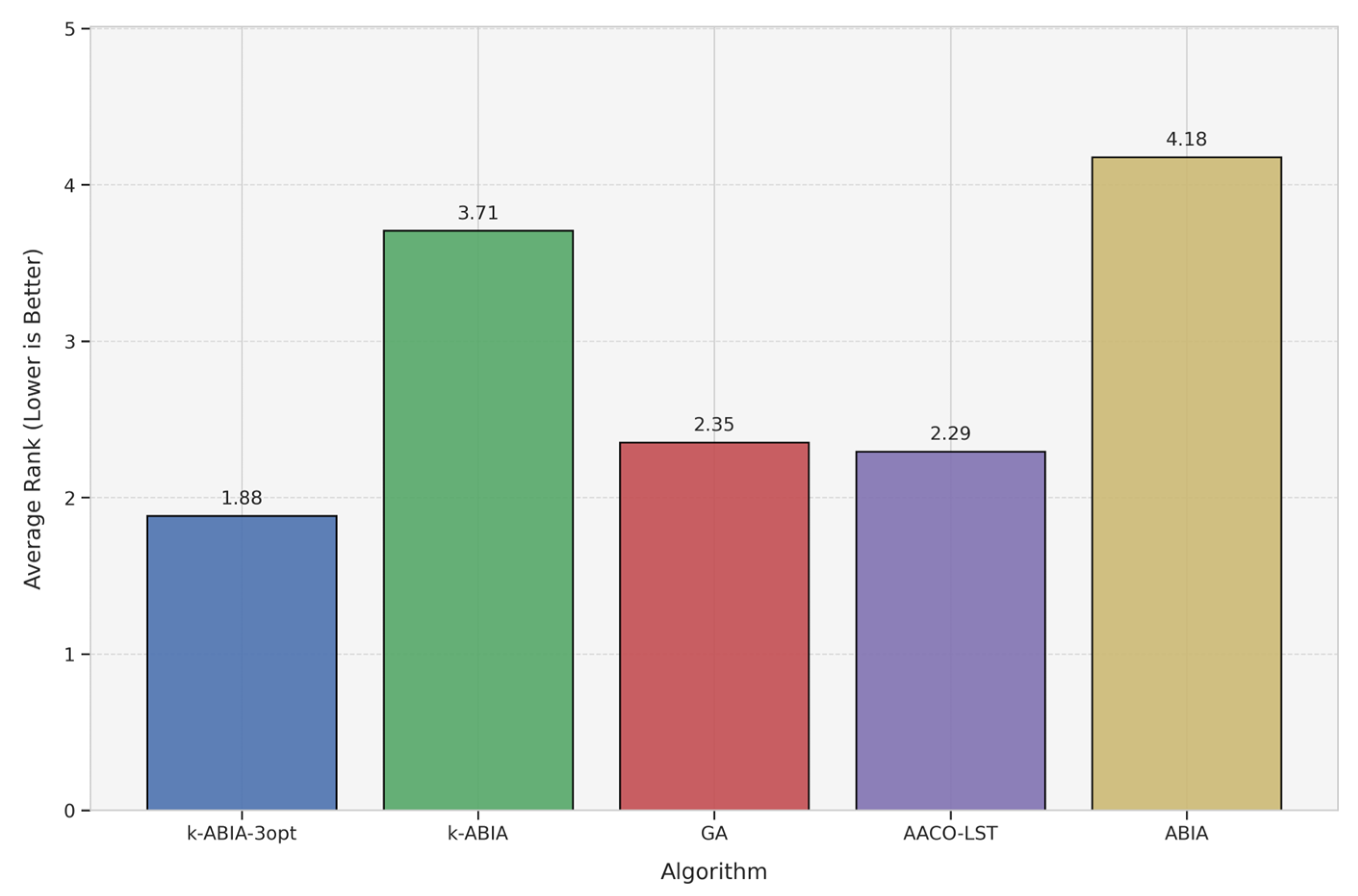
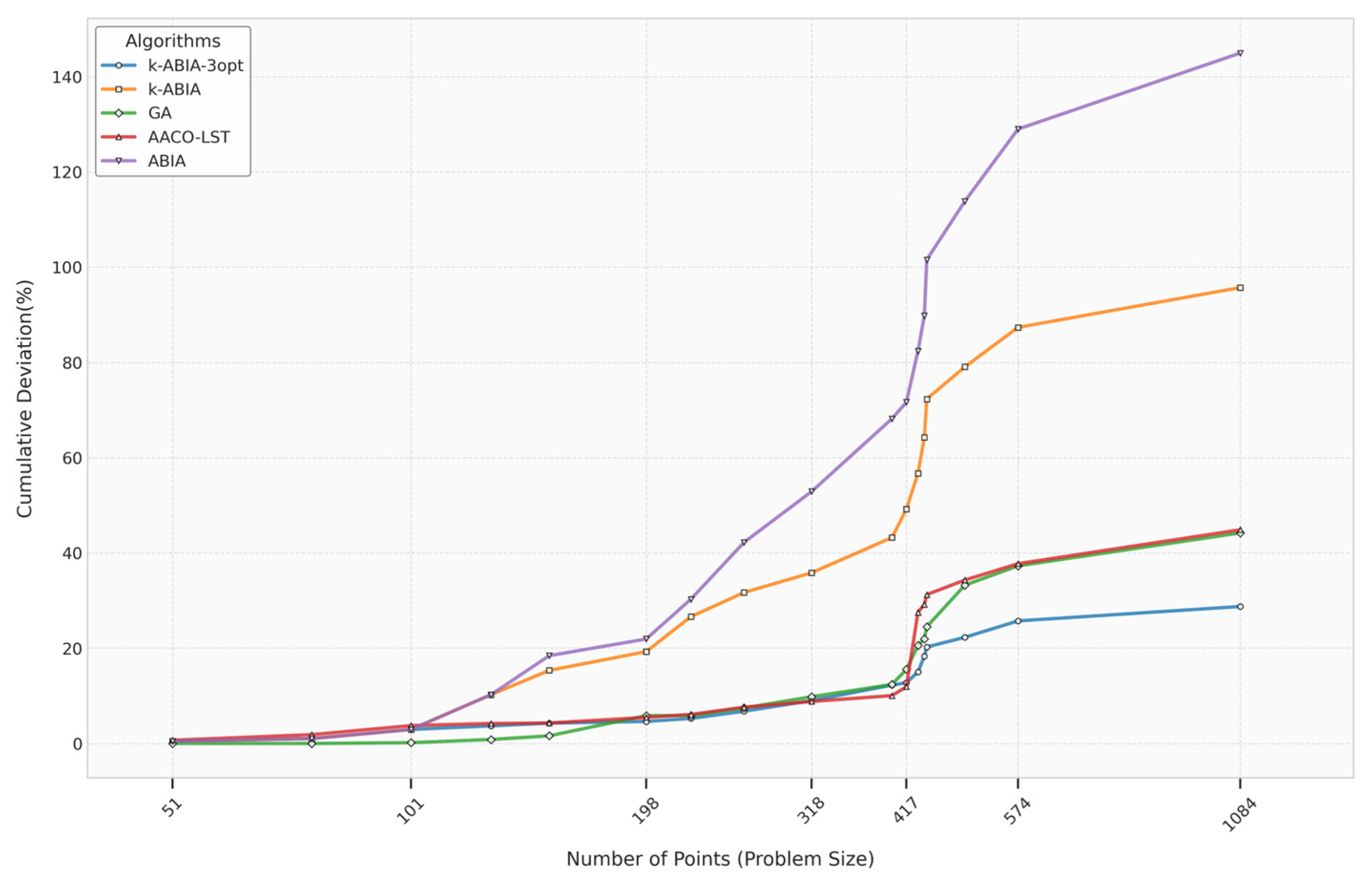
Furthermore, the average rank data from Table 3 were used to generate the histogram (Figure 7), while the BSD (Best Solution Deviation) values listed in Table 2 were used to construct the cumulative deviation plot (Figure 8). Together, Figure 7 and Figure 8, along with the tabulated results in Table 3 and

Table 4. Performance and stability on TSP instances.

Instance (Optimum)	Cities	Algorithm	Best	Avg	Worst	Std	CV
ch130(6110)	130	k-ABIA-3opt	6235	6235	6235	0	0.00%
		k-ABIA	6431	6431	6431	0	0.00%
		GA	6170	7329.44	8534	775.11	10.58%
kroA200(29,368)	200	k-ABIA-3opt	30,350	30,467.56	30,623	116.47	0.38%
		k-ABIA	31,436	31,436	31,436	0	0.00%
		GA	29,505	31,914.10	36,128	1948.98	6.11%
pr226(80,369)	226	k-ABIA-3opt	80,839	84,447.80	87,058	2212.62	2.62%
		k-ABIA	83,571	88,711.16	90,370	2481.43	2.80%
		GA	80,882	98,893.14	122,314	11,343.58	11.47%
pr299(48,191)	299	k-ABIA-3opt	49,012	49,701.84	50,501	419.42	0.84%
		k-ABIA	51,176	51,927.60	53,954	993.55	1.91%
		GA	49,280	56,871.28	65,010	4783.58	8.41%
lin318(42,029)	318	k-ABIA-3opt	42,972	43,314.92	43,696	166.32	0.38%
		k-ABIA	43,770	44,853.96	45,130	310.89	0.69%
		GA	43,021	51,566.58	60,311	5159.46	10.01%
gr431(171,414)	431	k-ABIA-3opt	175,303	177,320.44	183,668	2264.81	1.28%
		k-ABIA	184,261	188,354.20	198,086	4517.16	2.40%
		GA	180,023	212,970.36	253,633	20,663.48	9.70%
ali535(202,339)	535	k-ABIA-3opt	209,332	210,975.88	212,498	955.36	0.45%
		k-ABIA	218,207	221,288.10	230,074	3179.08	1.44%
		GA	209,331	239,082.32	275,124	19,333.56	8.09%
rat783(8806)	783	k-ABIA-3opt	9109	9184.20	9254	41.93	0.46%
		k-ABIA	9596	9677.64	9739	31.90	0.33%
		GA	9160	10,423.10	11,448	642	6.16%
pr1002(259,045)	1002	k-ABIA-3opt	267,521	269,849.16	272,269	1089.77	0.40%
		k-ABIA	281,128	286,241.32	290,857	2394.59	0.84%
		GA	289,951	323,338.88	354,289	19,343.21	5.98%

, form the foundation for the following key observations:

• Across the 17 medium-to-large-scale TSP instances ranging from 51 to 1084 cities, the k-ABIA-3opt not only achieved the top average rank but also produced the best solutions in 7 instances—both metrics highlighting its superior solution quality compared to the other evaluated algorithms.
• The cumulative deviation of the k-ABIA-3opt was 66.95% lower than that of the k-ABIA, clearly demonstrating the effectiveness of local search strategies applied after clustering. Additionally, the cumulative deviation of k-ABIA was 49.23% lower than that of the original ABIA, confirming that the clustering–connection strategy significantly improves solution quality.

5.2. Assessment of Algorithmic Stability

In this subsection, TSP instances ranging from 100 to 1000 cities were randomly selected for evaluation. Both k-ABIA and k-ABIA-3opt include a single source of randomness—namely, the initial centroid selection in K-means clustering. These two algorithms were compared against GA, a representative metaheuristic method. ABIA, being a fully deterministic rule-based algorithm, was excluded from this comparison. For each instance, the best, average, and worst solutions were recorded, along with the standard deviation (Std) and coefficient of variation (CV), defined as follows:

$$Std=\sqrt{{\displaystyle \frac{{\displaystyle {\sum }_{i=1}^N{\left(x_i-\mu \right)}^2}}{N}}}$$

(19)

$$CV={\displaystyle \frac{Std}{\mu }}\times 100\%$$

(20)

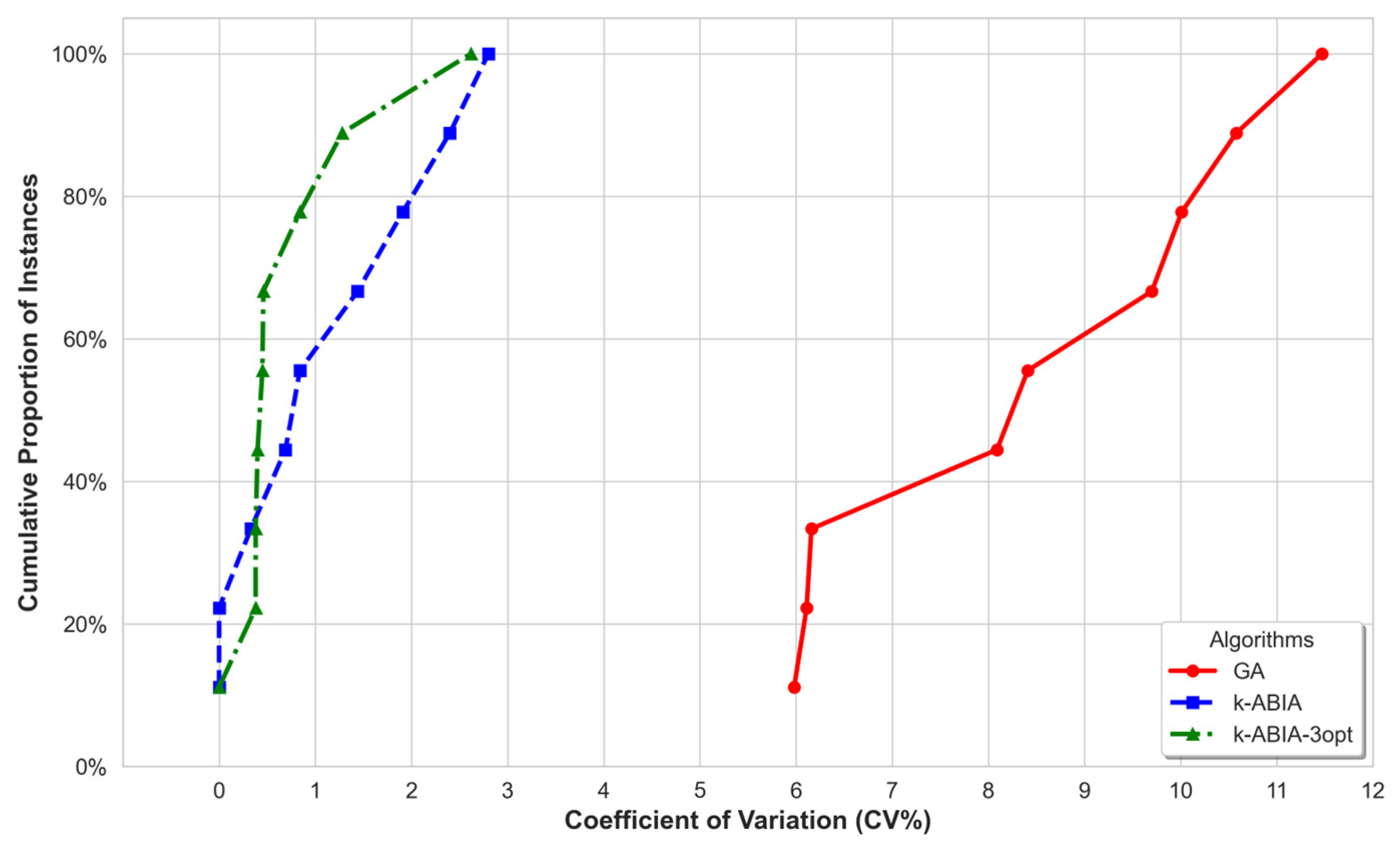
where N denotes the total number of solutions, $\mu$ is the average (Avg), and $x_i$ is the $i^{th}$ solution. Table 4 reports the stability comparison among algorithms. Figure 9 shows the cumulative distribution of CV values. From Table 4 and Figure 9, the following observations can be made:

• In all tested instances, the average and worst solution values obtained using k-ABIA-3opt were consistently better than those of the comparative algorithms, reflecting its advantage in both solution quality and stability.
• In Figure 7, the k-ABIA-3opt curve is concentrated near the left (low CV), with 80% of its CV values below 1%. Both k-ABIA-3opt and k-ABIA kept CV values under 3% across all instances, reflecting strong stability.

5.3. Analysis of Computational Efficiency

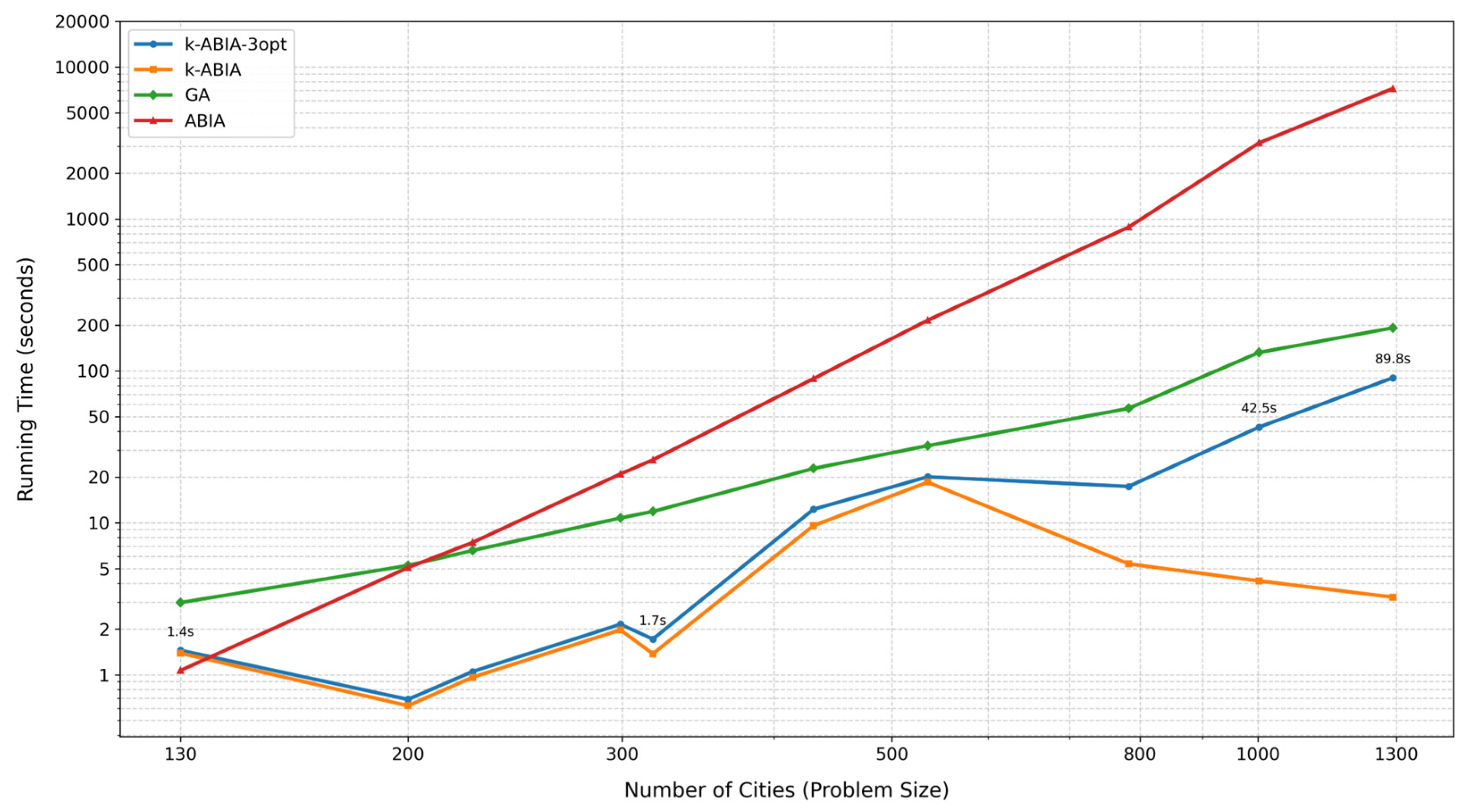
In this subsection, ten TSP instances ranging from 100 to 1300 cities were selected for evaluating the computational efficiency of the algorithms. Since the AACO-LST paper did not report runtime, only k-ABIA-3opt, k-ABIA, GA, and ABIA were compared. The results are shown in

Table 5. Comparative analysis of computational times across TSP instances.

Instance	Cities	Time (s)
		k-ABIA-3opt	k-ABIA	GA	ABIA
ch130	130	1.447	1.385	2.983	1.066
kroA200	200	0.687	0.624	5.232	5.067
pr226	226	1.048	0.962	6.563	7.416
pr299	299	2.146	1.969	10.740	20.928
lin318	318	1.715	1.374	11.859	25.934
gr431	431	12.250	9.561	22.742	88.730
ali535	535	20.058	18.493	32.127	214.892
rat783	783	17.336	5.358	56.583	883.102
pr1002	1002	42.548	4.142	131.935	3160.319
d1291	1291	89.848	3.239	191.735	7206.912
Total		189.083	47.108	472.497	11,614.367

, and the runtime trend with increasing problem size is illustrated in Figure 10. The key findings are summarized as follows:

• k-ABIA achieved the shortest runtime across all instances, with a maximum of only 18 s. In comparison, the total runtime of k-ABIA was approximately one-fourth of k-ABIA-3opt, one-tenth of GA, and just 1⁄61 of ABIA.
• A noticeable runtime spike was observed for ABIA on the gr431 instance. This is due to unbalanced k-means clustering in that instance, where one cluster contained over 200 cities, resulting in an expensive individual ABIA execution.

Based on the algorithmic characteristics, the theoretical time complexity of ABIA is $O\left(n^3\right)$, while GA has a complexity of $O\left(T{n}_0{n}^2\right)$ [31], where $n_0$ is the initial population size and T is the number of iterations. ABIA’s runtime exceeded GA’s when the number of cities surpassed 210, consistent with its higher computational complexity. Although k-ABIA-3opt also has a theoretical complexity of $O\left(n^3\right)$, its actual runtime was significantly reduced due to the clustering-and-partitioning strategy, which effectively narrows the 3-opt search space. k-ABlA does not utilize the 3-opt optimization path, so its time complexity is $O\left(n^2\right)$. Since k-ABlA has much smaller constant factors compared to GA, its running speed is faster.

5.4. Performance Evaluation of Asymmetric TSP Instances

In this subsection, since both k-ABIA-3opt and k-ABIA incorporate inter-cluster connection and path optimization rules specifically designed for ATSPs, we evaluated their solution quality on all ATSP instances with more than 100 cities from the TSPLIB benchmark. The AACO-LST algorithm was not designed for ATSPs and therefore was excluded from comparison. The comparison was carried out among k-ABIA-3opt, k-ABIA, GA, and ABIA. As established in Section 4, both k-ABIA-3opt and k-ABIA exhibit lower time complexity in ATSP than in TSP, and their runtime stability remains consistent with that observed in Section 5.2; hence, only solution quality is evaluated in this subsection.

Table 6. Performance comparison of algorithms on ATSP instances.

Instance	Cities	Algorithm	Best (BSD)	Rank
kro124p(36,230)	124	k-ABIA-3opt	38,319(5.77%)	2
		GA	36,724(1.36%)	1
		k-ABIA	38,609(6.57%)	3
		ABIA	38,609(6.57%)	3
ftv170(2755)	171	k-ABIA-3opt	2946(6.93%)	1
		GA	3208(16.44%)	3
		k-ABIA	3080(11.80%)	2
		ABIA	3235(17.42%)	4
rbg323(1326)	323	k-ABIA-3opt	1364(2.87%)	1
		GA	2343(76.70%)	4
		k-ABIA	1855(39.89%)	3
		ABIA	1648(24.28%)	2
rbg358(1163)	358	k-ABIA-3opt	1229(5.67%)	1
		GA	2214(90.37%)	3
		k-ABIA	2235(92.18%)	4
		ABIA	1605(38.01%)	2
rbg403(2465)	403	k-ABIA-3opt	2507(1.70%)	1
		GA	3916(58.86%)	4
		k-ABIA	3373(36.84%)	3
		ABIA	2606(5.72%)	2
rbg443(2720)	443	k-ABIA-3opt	2767(1.73%)	1
		GA	4540(66.91%)	4
		k-ABIA	3645(34.01%)	3
		ABIA	2947(8.35%)	2

reports the best solution deviations (BSDs) and rankings across ATSP instances, while

Table 7. Aggregate performance statistics of ATSP instances.

Algorithm	Rank1	Rank2	Rank3	Rank4	Average Rank	Total BSD
k-ABIA-3opt	5	1	0	0	1.17	24.67%
k-ABIA	0	1	4	1	3	221.29%
GA	1	0	2	3	3.17	310.64%
ABIA	0	4	1	1	2.5	100.35%

summarizes the overall performance. From these results, we observe the following:

k-ABIA-3opt achieved the highest average rank across all ATSP instances, followed by ABIA, k-ABIA, and GA. Its total BSD was only 24%, approximately one-twelfth that of GA. This superior performance stems from the fact that k-ABIA-3opt, k-ABIA, and ABIA all incorporate ATSP-specific design strategies. The lower solution quality of k-ABIA relative to ABIA indicates that clustering, by itself, fails to enhance solution quality in ATSP tasks. This further underscores the effectiveness of integrating a dedicated local search mechanism, as employed in k-ABIA-3opt, in enhancing solution quality.

6. Conclusions

To address the issues of poor solution quality and high time complexity in ABIA for medium- to large-scale TSPs, this study proposes two improvement strategies: k-ABIA (which integrates k-means clustering with ABIA) and k-ABIA-3opt (which further incorporates 3-opt optimization). These strategies employ a “Divide-Conquer-Construct-Optimize” three-phase collaborative mechanism, balancing both efficiency and precision.

k-ABIA employs K-means to partition large-scale problems into subproblems, reducing the time complexity of ABIA from $O\left(n^3\right)$ to $O\left(n^2\right)$. It then leverages the advantages of ABIA for smaller-scale TSPs while avoiding the high cost of global search. For symmetric TSP instances, eight inter-cluster connection strategies were specifically designed to link the clusters formed by k-means, followed by 3-opt-based route optimization. For asymmetric TSPs (ATSPs), four directed connection strategies were developed for the clustered subproblems, with corresponding refinement procedures applied after connection to further enhance solution quality.

Experimental results show that in large-scale TSP instances (with 100–1000 cities), k-ABIA-3opt generally outperforms k-ABIA, GA, AACO-LST, and ABIA in terms of solution quality. Regarding stability, both k-ABIA-3opt and k-ABIA demonstrated superior robustness, due to their limited randomness (only in the selection of cluster centroids), compared to GA. In terms of runtime, k-ABIA was the fastest, followed by k-ABIA-3opt, GA, and ABIA. For ATSP instances, k-ABIA-3opt achieved the highest solution quality, surpassing k-ABIA, GA, and ABIA. These results suggest that k-ABIA-3opt is more suitable for time-constrained scenarios where high-quality solutions are required, while k-ABIA offers a more efficient alternative for fast approximate solutions in large-scale settings. Moreover, both k-ABIA and k-ABIA-3opt are effective extensions under large-scale ATSP conditions.

Future research could focus on the following directions:

• Dynamic Clustering Strategy: Adaptively adjusting cluster sizes based on path directional characteristics or point group density to improve the feasibility of inter-cluster connections in ATSP.
• Initial Point and Bisecting Strategy Optimization: ABIA’s solution quality is significantly influenced by the initial starting point and bisecting direction. Heuristic rules could be designed to precisely select initial points and optimize bisecting directions, reducing time complexity to $O\left(n^2\right)$.
• The proposed method holds promise for extension to other combinatorial optimization problems, such as the Vehicle Routing Problem, Quadratic Assignment Problem, and Job Shop Scheduling Problem, by appropriately adapting its clustering and refinement strategies. Furthermore, due to its structure-preserving and subset selection capabilities, the method also shows potential for application in feature selection tasks. These directions will be explored in future research.

References

1. Kaml, B.S.; Ibrahim, M.S. Solving the Multi-Objective Travelling Salesman Problem with Real Data Application. J. Al-Nahrain Univ. 2018, 21, 146–161. [Google Scholar] [CrossRef]
2. Macioszek, E.; Granà, A.; Fernandes, P.; Coelho, M.C. New Perspectives and Challenges in Traffic and Transportation Engineering Supporting Energy Saving in Smart Cities—A Multidisciplinary Approach to a Global Problem. Energies 2022, 15, 4191. [Google Scholar] [CrossRef]
3. ŞİRİN, M.; ALTINTAŞ, T.; GÜNEŞ, A. Creating the Best Routing by Heuristic Algorithm. Int. J. Eng. Technol. Manag. Res. 2020, 4, 28–42. [Google Scholar] [CrossRef]
4. Gutin, G.; Punnen, A.P. The Traveling Salesman Problem and Its Variations; Springer Science & Business Media: Berlin/Heidelberg, Germany, 2006; Volume 12, ISBN 0306482134. [Google Scholar]
5. Padberg, M.; Rinaldi, G. A Branch-and-Cut Algorithm for the Resolution of Large-Scale Symmetric Traveling Salesman Problems. SIAM Rev. 1991, 33, 60–100. [Google Scholar] [CrossRef]
6. Herraiz, A.; Gutierrez, M.; Ortega-Mier, M. Equivalent Cyclic Polygon of a Euclidean Travelling Salesman Problem Tour and Modified Formulation. Cent. Eur. J. Oper. Res. 2022, 30, 1427–1450. [Google Scholar] [CrossRef]
7. Kimura, K.; Higa, S.; Okita, M.; Ino, F. Accelerating the Held-Karp Algorithm for the Symmetric Traveling Salesman Problem. IEICE Trans. Inf. Syst. 2019, 102, 2329–2340. [Google Scholar] [CrossRef]
8. Babaee Tirkolaee, E.; Cakmak, E.; Karadayi-Usta, S. Traveling Salesman Problem with Drone and Bicycle: Multimodal Last-mile E-mobility. Int. Trans. Oper. Res. 2024, 32, 3232–3258. [Google Scholar] [CrossRef]
9. Mahmoudinazlou, S.; Kwon, C. A Hybrid Genetic Algorithm for the Min–Max Multiple Traveling Salesman Problem. Comput. Oper. Res. 2024, 162, 106455. [Google Scholar] [CrossRef]
10. Roberti, R.; Ruthmair, M. Exact Methods for the Traveling Salesman Problem with Drone. Transp. Sci. 2021, 55, 315–335. [Google Scholar] [CrossRef]
11. Tongur, V.; Ülker, E. The Analysis of Migrating Birds Optimization Algorithm with Neighborhood Operator on Traveling Salesman Problem. In Intelligent and Evolutionary Systems: The 19th Asia Pacific Symposium, IES 2015, Bangkok, Thailand, November 2015, Proceedings; Springer: Berlin/Heidelberg, Germany, 2015; pp. 227–237. [Google Scholar]
12. Razali, N.M.; Geraghty, J. Genetic Algorithm Performance with Different Selection Strategies in Solving TSP. In Proceedings of the World Congress on Engineering, London, UK, 6–8 July 2011; International Association of Engineers: Hong Kong, China, 2011; Volume 2, pp. 1–6. [Google Scholar]
13. Xu, Z.; Zhang, X. An Improve Grey Wolf Optimizer Algorithm for Traveling Salesman Problems. IAENG Int. J. Comput. Sci. 2024, 51, 602–612. [Google Scholar]
14. Kıran, M.S.; İşcan, H.; Gündüz, M. The Analysis of Discrete Artificial Bee Colony Algorithm with Neighborhood Operator on Traveling Salesman Problem. Neural Comput. Appl. 2013, 23, 9–21. [Google Scholar] [CrossRef]
15. Hlaing, Z.; Khine, M.A. Solving Traveling Salesman Problem by Using Improved Ant Colony Optimization Algorithm. Int. J. Inf. Educ. Technol. 2011, 1, 404–409. [Google Scholar] [CrossRef]
16. Wang, K.-P.; Huang, L.; Zhou, C.-G.; Pang, W. Particle Swarm Optimization for Traveling Salesman Problem. In Proceedings of the 2003 international conference on machine learning and cybernetics (IEEE cat. no. 03ex693), Xi’an, China, 5 November 2003; Volume 3, pp. 1583–1585. [Google Scholar]
17. Cinar, A.C.; Korkmaz, S.; Kiran, M.S. A Discrete Tree-Seed Algorithm for Solving Symmetric Traveling Salesman Problem. Eng. Sci. Technol. Int. J. 2020, 23, 879–890. [Google Scholar] [CrossRef]
18. Pan, J.-S.; Ji, X.-F.; Liang, A.; Huang, K.-C.; Chu, S.-C. Parallel Binary Cat Swarm Optimization with Communication Strategies for Traveling Salesman Problem. J. Internet Technol. 2021, 22, 1621–1633. [Google Scholar]
19. Du, Z.-G.; Pan, J.-S.; Chu, S.-C.; Chiu, Y.-J. Multi-Group Discrete Symbiotic Organisms Search Applied in Traveling Salesman Problems. Soft Comput. 2022, 26, 4363–4373. [Google Scholar] [CrossRef]
20. Bresson, X.; Laurent, T. The Transformer Network for the Traveling Salesman Problem. arXiv 2021, arXiv:2103.03012. [Google Scholar] [CrossRef]
21. Zhao, K.; Liu, S.; Yu, J.X.; Rong, Y. Towards Feature-Free TSP Solver Selection: A Deep Learning Approach. In Proceedings of the 2021 International Joint Conference on Neural Networks (IJCNN), Shenzhen, China, 18–22 July 2021; pp. 1–8. [Google Scholar]
22. Lamperti, R.D.; de Arruda, L.V.R. A Strategy Based on Wave Swarm for the Formation Task Inspired by the Traveling Salesman Problem. Eng. Appl. Artif. Intell. 2023, 126, 106884. [Google Scholar] [CrossRef]
23. Alipour, M.M.; Razavi, S.N.; Feizi Derakhshi, M.R.; Balafar, M.A. A Hybrid Algorithm Using a Genetic Algorithm and Multiagent Reinforcement Learning Heuristic to Solve the Traveling Salesman Problem. Neural Comput. Appl. 2018, 30, 2935–2951. [Google Scholar] [CrossRef]
24. Duman, T.; Duman, E. Solving a New Application of Asymmetric TSP by Modified Migrating Birds Optimization Algorithm. Evol. Intell. 2024, 17, 1697–1713. [Google Scholar] [CrossRef]
25. Xia, T. The Use of Big Data in the Take-out and Delivery Market in China. Front. Manag. Sci. 2023, 2, 26–55. [Google Scholar] [CrossRef]
26. Hui, L.; Min, C. Research on the Distribution System Simulation of Large Company’s Logistics under Internet of Things Based on Traveling Salesman Problem Solution. Cybern. Inf. Technol. 2016, 16, 891. [Google Scholar] [CrossRef]
27. Romero, M.C.; Sánchez, J.N.; Lira, D.A.; Talavera, J.G.C.; Urbano, J.A. Aplicación Del Modelo TSP En La Planificación de Rutas de Una Empresa de Servicio de Limpieza. Científica 2023, 27, e270103. [Google Scholar] [CrossRef]
28. Hurkens, C.A.J.; Woeginger, G.J. On the Nearest Neighbor Rule for the Traveling Salesman Problem. Oper. Res. Lett. 2004, 32, 1–4. [Google Scholar] [CrossRef]
29. Renaud, J.; Boctor, F.F.; Ouenniche, J. A Heuristic for the Pickup and Delivery Traveling Salesman Problem. Comput. Oper. Res. 2000, 27, 905–916. [Google Scholar] [CrossRef]
30. Alipour, M.M.; Razavi, S.N. A New Local Search Heuristic Based on Nearest Insertion into the Convex Hull for Solving Euclidean TSP. Int. J. Oper. Res. 2019, 34, 409–429. [Google Scholar] [CrossRef]
31. Lin, J.; Zeng, X.; Liu, J.; Li, K. Angular Bisector Insertion Algorithm for Solving Small-Scale Symmetric and Asymmetric Traveling Salesman Problem. J. Comb. Optim. 2022, 43, 235–252. [Google Scholar] [CrossRef]
32. Croes, G.A. A Method for Solving Traveling-Salesman Problems. Oper. Res. 1958, 6, 791–812. [Google Scholar] [CrossRef]
33. Baydogmus, G.K. Solution for TSP/MTSP with an Improved Parallel Clustering and Elitist ACO. Comput. Sci. Inf. Syst. 2023, 20, 195–214. [Google Scholar] [CrossRef]
34. Latah, M. Solving Multiple TSP Problem by K-Means and Crossover Based Modified ACO Algorithm. Int. J. Eng. Res. Technol. 2016, 5, 430–434. [Google Scholar]
35. Mahi, M.; Baykan, Ö.K.; Kodaz, H. A New Hybrid Method Based on Particle Swarm Optimization, Ant Colony Optimization and 3-Opt Algorithms for Traveling Salesman Problem. Appl. Soft Comput. J. 2015, 30, 484–490. [Google Scholar] [CrossRef]
36. Liu, J.; Feng, M.; Xiu, X.; Liu, W. Towards Robust and Sparse Linear Discriminant Analysis for Image Classification. Pattern Recognit. 2024, 153, 110512. [Google Scholar] [CrossRef]
37. Rauf, A.; Sheeba, S.M.; Khusro, S.; Javed, H. Enhanced K-Mean Clustering Algorithm to Reduce Number of Iterations and Time Complexity. Middle-East. J. Sci. Res. 2012, 12, 959–963. [Google Scholar]
38. Lancia, G.; Dalpasso, M. Finding the Best 3-OPT Move in Subcubic Time. Algorithms 2020, 13, 306. [Google Scholar] [CrossRef]
39. Tang, K.; Wei, X.F.; Jiang, Y.H.; Chen, Z.W.; Yang, L. An Adaptive Ant Colony Optimization for Solving Large-Scale Traveling Salesman Problem. Mathematics 2023, 11, 4439. [Google Scholar] [CrossRef]
40. Reinelt, G. TSPLIB—A Traveling Salesman Problem Library. ORSA J. Comput. 1991, 3, 376–384. [Google Scholar] [CrossRef]
Figure 1. Construction of initial loop. (i) Construction of the angle bisector for the sector; (ii) Strategy for determining the initial connection point; (iii) Formation of the initial loop for the TSP; (iv) Formation of two initial directed loops for the ATSP.
Symmetry 17 01345 g001
Figure 2. The eight connection methods of 3-opt. In each method, the points represent cities in the TSP, and the loops are formed by disconnecting and reconnecting edges. The dashed lines represent the edges that are being swapped or removed, while the solid lines represent the edges that remain unchanged. Each subfigure (ah) shows a different way of breaking and reconnecting edges to create a new loop.
Symmetry 17 01345 g002
Figure 3. The eight connection methods between TSP clusters. In the figure, circles represent points of one cluster, triangles represent points of another cluster, and red dashed lines indicate connections between the two clusters. ①–⑧ represent different inter-cluster connection methods.
Symmetry 17 01345 g003
Figure 4. The four connection methods between ATSP clusters. We’ve added explanations for Figure 4: Circles represent connection points of one cluster, triangles represent points to be connected of the other cluster, red dashed lines are inter - cluster connection lines, arrows indicate directions, and ①–④ represent 4 different inter-cluster connection methods.
Symmetry 17 01345 g004
Figure 5. Modified 3-opt for ATSP. In the figure, circles represent TSP points. Red dashed lines indicate disconnections and reconnections to form new circuits. Arrows represent directions, showing the process of the modified 3—opt operation for the ATSP.
Symmetry 17 01345 g005
Figure 6. A flowchart of the improved Angular Bisector Algorithm combining K-means and 3-opt.
Symmetry 17 01345 g006
Figure 7. Histogram of average ranks of algorithms.
Symmetry 17 01345 g007
Figure 8. Cumulative Best Solution Deviation diagram across all instances.
Symmetry 17 01345 g008
Figure 9. Cumulative distribution of CV values across TSP instances.
Symmetry 17 01345 g009
Figure 10. Runtime scaling of algorithms with increasing TSP size.
Symmetry 17 01345 g010