Abstract
With the deep integration of Internet of Vehicles (IoV) and edge computing technologies, the spatiotemporal dynamics, burstiness, and load fluctuations of user requests pose severe challenges to microservices auto-scaling. Existing static or periodic resource adjustment strategies struggle to adapt to IoV edge environments and often neglect service dependencies and multi-objective optimization synergy, failing to fully utilize implicit regularities like the symmetry in spatiotemporal patterns. This paper proposes a dual-phase dynamic scaling mechanism: for long-term scaling, the Spatio-Temporal Graph Transformer (STGT) is employed to predict traffic flow by capturing correlations in spatial–temporal distributions of vehicle movements, and the improved Multi-objective Graph-based Proximal Policy Optimization (MGPPO) algorithm is applied for proactive resource optimization, balancing trade-offs among conflicting objectives. For short-term bursts, the Fast Load-Aware Auto-Scaling algorithm (FLA) enables rapid instance adjustment based on the M/M/S queuing model, maintaining balanced load distribution across edge nodes—a feature that aligns with the principle of symmetry in system design. The model comprehensively considers request latency, resource consumption, and load balancing, using a multi-objective reward function to guide optimal strategies. Experiments show that STGT significantly improves prediction accuracy, while the combination of MGPPO and FLA reduces request latency and enhances resource utilization stability, validating its effectiveness in dynamic IoV environments.
1. Introduction
With the deepening integration of Internet of Vehicles [1,2,3] (IoV) and edge computing technologies [4,5,6], data interaction between vehicles and infrastructure has become increasingly frequent, posing greater challenges to service response speed, system elasticity, and resource utilization efficiency. Microservice architecture [7], due to its modular, loosely coupled, and scalable characteristics, has been widely adopted in vehicular network scenarios. By decomposing complex applications into multiple independent services that collaborate through lightweight communication mechanisms, microservices [8,9] significantly enhance system flexibility and adaptability. This architecture has demonstrated strong performance in applications such as vehicle navigation, intelligent perception, and edge computing [10].
However, most existing research on microservices auto-scaling still relies on static or periodic strategies for resource adjustment, which are ill-suited to the spatiotemporal variability, burstiness, and dynamic load fluctuations typical of user requests in vehicular edge computing environments [11,12]. For instance, some studies make scaling decisions based solely on single metrics like CPU or memory usage [13,14], neglecting critical factors such as request latency, quality of service (QoS), and resource heterogeneity across edge nodes, which leads to suboptimal resource utilization or excessive delays. Other works attempt to introduce prediction-based scaling mechanisms [15,16], but often rely on linear or stationary assumptions that fail to capture the complex spatiotemporal correlations inherent in vehicular network scenarios. Moreover, mainstream orchestration platforms such as Kubernetes typically use threshold-based horizontal pod autoscaling (HPA), which suffers from delayed responses and is ineffective under sudden traffic surges [17]. Although some studies have explored combining reinforcement learning with predictive models for intelligent scaling [18], many overlook inter-service dependencies and variations in service call paths, resulting in low training efficiency, poor generalization, and limited adaptability to the dynamic nature of vehicular edge computing. Therefore, there is an urgent need for a fine-grained auto-scaling mechanism that comprehensively considers spatiotemporal load dynamics, service dependency structures, and heterogeneous edge resource states to enable more efficient and intelligent elastic management of microservices.
To achieve efficient elastic management of microservice systems in vehicular edge computing environments, this paper introduces a dynamic auto-scaling mechanism that combines predictive analytics with reinforcement learning. However, applying advanced machine learning techniques to microservice auto-scaling presents several challenges. First, user requests in vehicular scenarios exhibit significant spatiotemporal non-uniformity and burstiness; changes in traffic flow directly affect service loads, making traditional static or periodic scaling strategies insufficient to meet real-time requirements. Second, microservices’ resource demands show dynamic fluctuations during operation; frequent scaling can lead to system instability and resource wastage. Finally, under high-concurrency conditions, ensuring rapid responses to load changes while maintaining service quality remains a key challenge in designing effective auto-scaling mechanisms.
To address these challenges, this paper proposes a dual-phase dynamic microservice scaling mechanism that integrates long-term trend prediction with short-term load awareness. On a longer time scale, future request loads are modeled using a Spatio-temporal Graph Transformer (STGT), and the improved Multi-objective Graph-based Proximal Policy Optimization (MGPPO) algorithm is employed to optimize scaling decisions. On a shorter time scale, a Fast Load-Aware Auto-Scaling algorithm (FLA) is designed to rapidly adjust instance counts when sudden traffic spikes occur, thereby ensuring system stability and response performance.
The main contributions of this study are summarized as follows:
- (1)
- To address spatiotemporal dynamics, burstiness, and load fluctuations of user requests in vehicular edge environments, we propose a dynamic microservice scaling model. It considers request latency and resource consumption, formulates a multi-objective optimization problem, adjusts instance counts across heterogeneous edge nodes based on load changes, and enhances system adaptability and resource utilization.
- (2)
- To better handle the non-stationary traffic patterns characteristic of vehicular networks, we improve upon the traditional Proximal Policy Optimization (PPO) algorithm by introducing the MGPPO algorithm. Leveraging dynamic masking mechanisms and topological embedding techniques, MGPPO enhances training efficiency and generalization capability in complex state spaces, effectively addressing the issue of delayed scaling decisions caused by conventional methods under fluctuating traffic conditions.
- (3)
- To handle sudden high-concurrency requests that may occur in the IoV environment, we specifically designed the FLA algorithm, which can respond and dynamically adjust resource allocation within seconds to ensure system stability and response performance. Experimental results show that compared with mainstream algorithms such as DDQN, SAC, and G_DDPG, the proposed method combining MGPPO with FLA performs better in terms of response delay control and load balancing. This provides new ideas and technical means for elastic management of microservices in the edge computing environment of the IoV, and lays a solid foundation for intelligent scheduling and optimization of service resources in future intelligent transportation systems.
2. Related Work
This section reviews research progress in traffic flow prediction and microservice scaling. With the deep integration of IoV and edge computing, vehicular networks demand higher service response efficiency, system elasticity, and resource utilization. As key to system stability, traffic flow dynamics and microservice elastic scaling have gained significant research attention. However, existing works have limitations in complex scenarios, making it necessary to sort out related research to lay the groundwork for better solutions in IoV edge environments.
2.1. Traffic Flow Prediction
Hochreiter et al. [19] proposed the Long Short-Term Memory (LSTM) network, which leverages a gating mechanism to effectively capture long-term dependencies in time series—proving valuable for modeling the temporal features of traffic flow. Wang et al. [20] conducted traffic flow prediction from a global perspective and provided reasonable traffic signal timing strategies based on such predictions. Through data analysis to forecast future road traffic flow and formulate corresponding optimal traffic signal strategies, their study put forward a time series prediction method based on recurrent neural networks (TSPR). Li et al. [21] introduced the Diffusion Convolutional Recurrent Neural Network (DCRNN), which models information propagation in traffic networks via bidirectional random walks and incorporates a Seq2Seq structure for temporal modeling. This approach is capable of capturing both temporal and spatial dependencies. Zhao et al. [22] explored the problem of traffic flow forecasting and proposed a novel model, Dynamic Hypergraph Structure Learning (DyHSL), for traffic flow prediction. Yu et al. [23] developed the Spatio-Temporal Graph Convolutional Network (STGCN), which merges graph convolution and temporal convolution to efficiently extract spatio-temporal features from traffic flow data. Bai et al. [24] developed the Spatio-Temporal Graph-to-Sequence network (STG2Seq), integrating graph neural networks with Sequence-to-Sequence (Seq2Seq) models to enable concurrent modeling of both spatial and temporal dependencies within traffic flow data. Wu et al. [25] proposed Graph WaveNet, a model that achieves efficient spatio-temporal modeling of traffic flow data by fusing graph convolutional networks with one-dimensional extended causal convolution. It utilizes an adaptive graph learning mechanism to capture the dynamic topology of traffic networks without relying on predefined adjacency matrices.
Existing models have their own focuses in capturing spatio-temporal features and modeling dependencies, but there is still room for further optimization. Based on this, we innovatively adopt the STGT model for traffic flow prediction. This model integrates graph structures’ ability to accurately depict spatial correlations with Transformers’ advantage in efficiently capturing long-term temporal dependencies. It adapts to real-time changes in traffic networks by constructing dynamic graph structures that reflect real-time topological relationships and leverages self-attention mechanisms to deeply explore complex interactive relationships in spatio-temporal dimensions, with the expectation of improving the accuracy and robustness of traffic flow prediction.
2.2. Microservice Scaling
Li et al. [26] proposed a fuzzy-based microservice computing resource-scaling (FMCRS) algorithm that leverages fuzzy reasoning, particle swarm optimization, and expansion strategies to optimize microservice resource management in IoV edge computing environments. Zarie et al. [27], focusing on IoV scenarios with base station communication, combined fuzzy logic reasoning with priority scheduling to achieve intelligent microservice scaling, demonstrating significant advantages over Kubernetes-based methods. Zhao et al. [28] proposed DDQN, a deep reinforcement learning-based approach for online microservice deployment. Specifically, DDQN employs the Dueling DQN (Deep Q-Network) model to dynamically generate real-time deployment strategies in response to fluctuating system loads and resource demands. Santos et al. [29] introduced the gym-hpa framework, which applies reinforcement learning to study the impact of microservice dependencies on auto-scaling, aiming to reduce both resource consumption and request latency. Samanta et al. [30] proposed the Dyme algorithm, which formulates a multi-objective optimization model and employs a multi-queue feedback priority scheduling scheme to address dynamic microservice scheduling in IoT mobile edge computing. Wang et al. [31] introduced the elastic scheduling for microservices algorithm (ESMS), which jointly optimizes microservice task scheduling and resource scaling to minimize virtual machine rental costs while meeting task deadlines. Tuli et al. [32] proposed an asynchronous advantage actor–critic (A3C)-based real-time scheduler for stochastic Edge-Cloud environments. Using the Residual Recurrent Neural Network (R2N2) architecture, it enables decentralized learning across multiple agents, capturing host and task parameters along with temporal patterns for efficient scheduling. Toka et al. [17], targeting Kubernetes-based edge clusters, integrated multiple machine learning techniques to build a prediction engine, addressing the limitation of Kubernetes’ default scaling mechanism in proactively adapting to workload fluctuations. Rossi et al. [33] proposed a reinforcement learning-based dynamic multi-metric threshold algorithm for microservice elasticity, employing an adaptive multi-metric threshold strategy under both single-agent and multi-agent architectures. Li et al. [34] proposed an edge service placement strategy based on an improved NSGA-II, called GA-MSP, which minimizes transmission delay and load imbalance under the constraint of one container per service instance. Shifrin et al. [35] presented a Markov Decision Process (MDP)-based method for dynamic virtual machine scaling and load balancing, constructing an MDP model to optimize system cost and revenue, and also introduced an abstract MDP approach to handle large-scale scenarios. Garg et al. [36], targeting dynamic service placement in mobile edge computing, proposed an optimization method combining heuristic algorithms with deep deterministic policy gradient (DDPG) reinforcement learning to address the challenges posed by user mobility and resource dynamics.
Most existing studies on microservice dynamic scaling are based on static or semi-static request patterns, making them difficult to adapt to the time-varying nature of traffic in mobile edge environments. Methods such as FMCRS and ESMS have similar limitations, exhibiting delayed responses to traffic fluctuations and easily causing service quality degradation under sudden traffic surges.
Specifically, FMCRS relies on 27 manually defined fuzzy rules to classify CPU and memory loads. Despite optimization via the Particle Swarm Optimization (PSO) algorithm, its rule-driven nature makes it unable to capture the complex spatiotemporal dynamics of traffic in the IoV, resulting in rigid resource allocation. ESMS, while integrating task scheduling and auto-scaling, limits its decision-making to current states and lacks the ability to predict future traffic changes. During sudden traffic surges, it can only trigger scaling after the load exceeds a threshold, leading to delayed responses. Moreover, its cloud-oriented two-layer scaling mechanism (containers–virtual machines) is incompatible with the rapid changes in edge environments.
In contrast, our method autonomously learns the spatiotemporal dependencies of traffic through the STGT, eliminating the need for manual rule presets and enabling more accurate adaptation to dynamic loads. It combines the FLA algorithm to respond to sudden traffic in real time, effectively overcoming lag issues. Additionally, it captures service dependencies via graph convolutional networks and integrates dynamic weight routing strategies, significantly improving performance in multi-service collaboration scenarios.
In this paper, we focus on the IoV edge computing environment and investigate the problem of microservice dynamic scaling under dynamic request conditions. Our goal is to optimize request latency, load balancing, and resource utilization based on existing advanced methodologies. Unlike previous works, this paper presents an adaptive scaling method named MGPPO. It uses STGT for traffic prediction and includes graph convolutional networks. A FLA algorithm is also added to manage sudden traffic increases. This combination enables rapid instance adjustment, providing high-concurrency and low-latency service support in dynamic IoV environments.
3. Problem Formulation
This section formulates the problem of microservice dynamic scaling in the IoV edge computing environment, with the aim of addressing the challenges posed by the spatiotemporal dynamics, burstiness, and load fluctuations of user requests. We first describe the system scenario, then detail the STGT-based traffic flow prediction model and the microservice dynamic scaling framework, and finally clarify the constraints and optimization objectives, thereby laying a theoretical foundation for the subsequent algorithm design.
3.1. Scenarios
Figure 1 presents the architecture of microservice resource utilization and request flows in the IoV edge computing environment, with core components including base stations, edge servers, and vehicle–infrastructure interaction links, clearly illustrating the system’s physical connection topology and logical collaboration mechanisms.
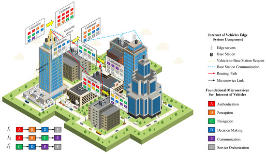
Figure 1.
The architecture of microservice resource utilization and request flows in the IoV edge computing environment.
As the core communication hub, base stations receive service requests sent by vehicles through wireless links and transmit data with edge servers via wired connections, forming a critical transmission path for requests from terminal devices to computing nodes. Edge server clusters deploy foundational IoV microservices and achieve inter-node collaborative communication through routing paths, providing distributed computing support for the operation of various core services.
Microservice types fully cover the core business needs of IoV: Authentication Service (A) is responsible for verifying vehicle identity and request legitimacy; Perception Service (B) processes roadside sensor data to achieve accurate environmental state perception; Navigation Service (C) provides dynamic route planning based on real-time traffic flow data; Decision Service (D) generates vehicle control suggestions based on perception and navigation information; Communication Service (E) focuses on optimizing cross-node data transmission efficiency; and Service Orchestration (F) flexibly adapts to dynamic changes in request loads by dynamically scheduling instances and coordinating service invocation chains. Request flows follow the transmission path of “vehicle → base station → edge server” and are intelligently allocated to corresponding microservice chains by the service orchestration module according to request types. For example, a navigation request triggers the collaborative process of “Authentication (A) → Perception (B) → Navigation (C) → Communication (E)”, ensuring targeted and efficient service responses. This architecture, with its distributed deployment and dynamic collaboration characteristics of microservices, lays a solid foundation for elastic resource management in the IoV edge environment.
3.2. STGT-Based Traffic Flow Prediction Model
3.2.1. Model Architecture
Figure 2 illustrates the overall architecture of STGT. This model integrates a Graph Convolutional Network (GCN) with the Transformer mechanism, specifically designed for spatio-temporal sequence prediction tasks such as traffic flow forecasting. Its structure mainly consists of an input layer, a spatio-temporal position embedding layer, an encoder, a decoder, and an output layer. The model input consists of three parts. The first is the adjacency matrix, which describes the relationships between nodes. The second and third parts are the encoder and decoder inputs. Both are spatio-temporal feature tensors with the shape . Here, n denotes the number of nodes, T represents the number of time steps, and F indicates the number of features.
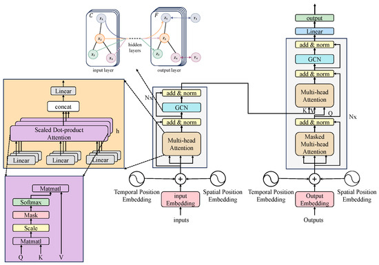
Figure 2.
STGT overall framework diagram.
The raw input is first projected through a Multi-Layer Perceptron (MLP) to enhance its representational capacity by mapping it into a fixed-dimensional space. The projected features are then combined with Temporal Position Embedding and Spatial Position Embedding before being fed into the encoder.
The encoder of STGT combines GCN with Multi-Head Self-Attention to jointly model spatial and temporal information. The GCN aggregates information from neighboring nodes using the adjacency matrix to update node representations, while the multi-head attention captures global dependencies within the time series, avoiding the gradient vanishing problem inherent in traditional RNN structures. Each layer incorporates residual connections and layer normalization to improve training stability.
During the decoding phase, the model fuses historical information to generate predictions for future time steps. Since the current prediction must not depend on future time steps, a Masked Attention mechanism is employed to mask out subsequent time-step information. Unlike conventional Transformers, STGT continues to use GCN instead of a standard feed-forward network during decoding, preserving spatial topological information and ensuring that predictions align with the actual structure of the transportation network.
3.2.2. Model Functional Module Architecture
- (1)
- Spatial Feature Extraction Module
In traffic flow prediction tasks, the traffic network is modeled as a weighted undirected graph , where V denotes the set of sensor nodes, E represents the edges between nodes, and A is the adjacency matrix that defines node connectivity.
To capture spatial dependencies, we employ GCNs as the spatial feature extraction module. The core operation of a GCN layer is defined as:
In this formulation, denotes the input feature matrix at the l-th GCN layer, and represents the learnable weight matrix at that layer. The activation function introduces non-linearity into the model, which helps improve its expressive power and training stability. The adjacency matrix is constructed by adding self-loops to the original adjacency matrix A, where I is the identity matrix. is the degree matrix of , with its diagonal elements defined as , representing the sum of weights for each node’s connections.
This formulation enables each node to aggregate information from its neighbors, thereby capturing broader spatial dependencies by integrating both local and structural features.
However, as the number of GCN layers increases, node representations tend to become overly smoothed, leading to reduced feature distinguishability—a phenomenon known as over-smoothing. To mitigate this issue and preserve feature discriminability, we introduce a residual connection after each GCN layer. This allows to retain part of the original input features, improving model expressiveness and training stability.
- (2)
- Temporal Feature Extraction Module
Considering the temporal characteristics of traffic flow data, this chapter employs the self-attention mechanism to model temporal dependencies. The self-attention computation is defined as follows:
where Q, K, and V denote the query, key, and value matrices derived from the input features, respectively, and is a scaling factor that prevents large values from destabilizing gradient computations.
Since single-head attention may overlook interactions across different time steps, we further adopt the multi-head attention (MHA) mechanism. Its formulation is given as:
where , , and are projection weight matrices for each head, and is the output weight matrix. X is an input tensor, representing feature data that includes dimensions such as time steps.
To further enhance the modeling of temporal information, we introduce temporal positional encoding into the architecture. The encoding is computed as follows:
where t represents the time step and denotes the hidden dimension of the model. and generate periodic encodings with different frequencies.
3.3. Microservice Dynamic Scaling Model
3.3.1. Transmission Model
In the IoV scenario, vehicles communicate with the base station through 5G wireless communication, and wired connections are used between the base station and MEC servers, and between MEC servers. Due to the limitation of sensor technology, only the number of vehicles within the detection range can be counted, so the fixed position of the sensor is used to refer to the position of all detected vehicles in the region. Because of the fixed position of the sensor and the base station, the propagation delay of the wireless transmission of the two is constant and a single connection can be maintained, without the need to repeat the construction of the connection delay while, at the same time, assuming that the processing capacity of the base station is unlimited and its queuing delay can be ignored. Therefore, this paper focuses on analyzing the transmission delay between the base station and MEC servers and between MEC servers, including the propagation delay, queuing delay, processing delay and the forwarding-related delay generated by the forwarding device. Specifically, the propagation delay can be expressed as:
where denotes the propagation delay, d is the total distance of the transmission medium (e.g., fiber-optic or coaxial cable) between the source and destination nodes, and v represents the signal propagation speed in that medium. Queuing delay, processing delay, and forwarding delay are typically associated with the number of forwarding hops, as they are all incurred during packet switching. Assuming that each forwarding device introduces a fixed delay of , the total forwarding delay across H hops can be expressed as:
This term captures the cumulative forwarding delay from the source to the destination. Additionally, a single-task execution delay, denoted by , is introduced to characterize the time overhead required for operations such as packet parsing, header checking, and route computation at each forwarding node. If the number of tasks waiting in the queue is , the queuing delay due to the serial processing mechanism becomes . This includes the delay caused by the one task currently being processed and the tasks waiting in the queue. Finally, the total transmission delay from the source to the destination can be expressed as:
This formulation systematically accounts for the delays due to physical signal propagation, intermediate node forwarding, and queuing plus processing at each hop.
3.3.2. Resource Model
A single cluster may contain one or more base stations. Let denote the set of base stations in the cluster, where n is the number of base stations. The geographic coordinates (longitude and latitude) of the n-th base station are represented by . Given that 5G base stations are typically deployed approximately 1 km apart, the MEC servers associated with a cluster should be placed as close as possible to the base stations in the network topology to minimize network latency. Therefore, only MEC servers located within a straight-line distance of 2 km from any base station in the cluster are allowed to join. Let represent the set of all MEC servers that are eligible to join the cluster — including both currently included and excluded servers — provided they meet the distance constraint. Furthermore, define , where as the set of MEC servers currently belonging to the cluster. Here, k denotes the total number of MEC servers under consideration. The geographical location of the k-th MEC server is denoted by .
Each MEC server consists of four types of computing resources: CPU, memory, storage (disk), and GPU. The initial resource capacities vary across different types of MEC servers. Let represent the overall resource profile of the MEC servers, where each individual server’s resource configuration is defined as . Let denote the set of microservice types, with s representing the total number of distinct microservice types. The required resource profile for these microservices is denoted by where the resource demand of a single microservice type is expressed as . The weight vector of all microservices is defined as , where denotes the weight assigned to the s-th microservice type.
Each MEC server in the set is assigned an independent computational capacity benchmark , based on its CPU core count and clock frequency. As the server load increases, its effective computing power decreases. We define the effective computing capacity as where the function is defined as:
where represents the threshold load level, and is an empirically fitted parameter indicating the degree to which load affects computational performance. Finally, the execution time of a task is modeled as:
where denotes the relative computational data size of the corresponding microservice—a measure of the data volume required for its execution.
3.3.3. Scaling and Routing Model
Scaling of microservice instances on MEC servers includes scaling up, scaling down, and migrating. Scaling up is to add or delete instances in the target server when the traffic increases, consuming resources to improve throughput; shrinkage is to reduce instances when the traffic decreases, releasing resources to avoid waste; and migration is to expand the capacity of the server in the new hotspot area first, and then gradually shut down the instances in the original location, which is essentially a combination of expansion and shrinkage. In practice, scaling usually involves only expansion and contraction, and migration, as an advanced strategy based on scaling, is used to adapt to temporal and spatial changes in traffic and optimize system performance and resource utilization.
In this paper, we adopt a probability-based microservice routing strategy: when requests flow from parent nodes (upstream microservices) to child nodes (downstream microservices), they are not preset with a fixed target, but are dynamically selected based on real-time probability distributions. After the microservice deployment is completed, the requests are distributed to the downstream instances for processing through probabilistic routing. For this reason, this paper proposes a probabilistic routing model based on dynamic weight adjustment, which can combine the propagation delay of the parent and child nodes, the queuing situation of the child nodes, and the load state to dynamically calculate the routing probability, in order to achieve the system delay optimization and computational load balancing. When an upstream microservice needs to route requests to one of multiple downstream microservices , the routing probability is computed by normalizing the parent–child weight , where denotes the set of all possible downstream nodes. The weight is determined by three factors: the transmission and forwarding delay between the parent and child node, the queuing delay of the corresponding service at the child node, and the load status of the child node. There are two types of parent–child relationships: one in which a base station (AP) acts as the parent and an MEC server as the child, and another in which both the parent and the child are MEC servers. In both cases, data transmission occurs over wired links. According to the communication model, the delay over a wired link mainly consists of transmission delay and forwarding-related delay.
The queuing delay at the child node is calculated as the product of the total expected number of services waiting in the queue and the average execution time of each service. Specifically, if represents the current average number of queued services and denotes the average execution time per service at the child node , then the expected queuing delay is:
The load status refers to the resource utilization of the child node. Based on the baseline computational capacity of the child node and its current resource usage, the expected service execution time can be derived using the resource model described in Equation (11), which accounts for how load affects computing performance. Finally, the routing probability for each path can be calculated as:
3.3.4. Constraints and Optimization Objectives
When the reinforcement learning agent decides to perform a microservice instance scaling-down operation on an edge computing node, the number of deployed instances of this type of microservice on that node must satisfy the constraint ; that is, the number of scaled-down microservice instances must not exceed the current number of deployed instances. Otherwise, the scaling-down operation fails, and the system maintains its existing state. If this constraint is met, the scaling-down is successful, and the computing resources are released accordingly. After a server completes the scaling-down operation, its remaining available amount of resources can be updated as:
The amount of resources released by scaling-down is added to the original remaining resources, further improving the resource utilization rate of the server and providing room for possible subsequent scaling-up or task scheduling.
When performing a scaling-up operation, since the physical resources of the edge computing node have a strict upper limit, the reinforcement learning agent must first evaluate the resource availability of the current node when deciding on scaling-up to ensure that the scaling-up does not exceed its hardware limitations. When considering the feasibility of scaling-up, the system needs to first calculate the amount of resources released by scaling-down and then determine whether the scaling-up operation is executable based on this. Specifically, if the node still has sufficient available resources after completing the scaling-down, such that: , then the scaling-up can be successfully executed, and the system will add new microservice instances to meet the growing request demand. Conversely, if the scaling-up request exceeds the available resources of the current node, the operation fails, and the system remains unchanged.
In this chapter, users are most concerned about request latency, which is also what service providers care most about in practical engineering. Therefore, this chapter first optimizes the global request latency. The specific optimization function and constraint conditions are as follows. The calculation related to request latency can be expressed as:
The constraint conditions that need to be satisfied are summarized as follows:
4. Algorithm
To address the challenges of dynamic scaling of microservices in the IoV edge computing environment, this chapter constructs a core algorithm system for a dual-phase dynamic scaling mechanism. First, combined with the spatiotemporal characteristics of user requests and service dependencies, the MGPPO algorithm integrating graph convolutional networks is designed. It filters out invalid operations through a dynamic masking mechanism, improves training efficiency and generalization ability in complex state spaces, and realizes long-term proactive resource optimization. Second, the FLA algorithm for short-term burst traffic scenarios is elaborated. Based on the M/M/S queuing model, it monitors queue and resource status in real time and completes instance adjustment within seconds to cope with high-concurrency impacts. The two algorithms work together, from the perspectives of long-term prediction and short-term perception, to achieve multi-objective optimization of request latency, resource consumption, and load balancing, providing a complete solution for elastic management of microservices in the IoV edge environment.
4.1. Microservice Scaling Algorithm Based on MGPPO
This paper improves upon the PPO algorithm to develop the MGPPO algorithm, motivated by two key factors. First, the topology of vehicular edge servers exhibits graph-structured data characteristics, which are difficult for traditional neural networks to model effectively. By introducing a graph convolutional network, we can aggregate neighborhood features and accurately capture transmission delays and resource competition between servers. Second, microservice scaling decisions are subject to strict physical constraints. The standard PPO algorithm tends to generate invalid actions during exploration, leading to inefficient learning. In contrast, the action masking mechanism filters out infeasible actions, significantly improving training efficiency, especially in the early stages.
4.1.1. State
The state space in reinforcement learning must comprehensively cover global system information, including key elements such as server locations, resource statuses, traffic distributions, and microservice deployment states, to provide a basis for the agent to formulate optimal decisions. To effectively capture the global characteristics of the system, this paper generates a state vector through a global average pooling operation, which uniformly aggregates the features of all servers. This design ensures that each server contributes equally to the state representation, enabling the model to accurately depict the overall characteristics of the entire system.
From a mathematical perspective, the global state can be expressed as a vector integrating multiple features:
where denotes the graph structure of MEC servers, with v as the set of nodes (servers), E as the set of edges (communication links), and A as the adjacency matrix; represents the graph convolutional network operation, which is used to extract spatial features of the graph and output node feature matrices; indicates the global average pooling operation, which ensures each server contributes equally to the state representation by aggregating features of all nodes; is the request queue information vector of each server, where is the queue length of the i-th server; and ⊕ denotes the vector concatenation operation.
4.1.2. Action
In the scaling and routing model proposed in this paper, the scaling actions are explicitly defined as two types: scale-down and scale-up. The action space can be expressed as:
where s denotes the selected MEC server from the cluster; m represents the type of microservice; and is the scaling amount for microservice m on server s, with positive values indicating scale-up and negative values indicating scale-down.
Considering the sensing capabilities of traffic detectors and the deployment latency of container instances in engineering practice, the adjustment cycle is set to 5 min. Based on traffic flow predictions, the request stream data for the next 5 min is obtained in advance. Therefore, the reinforcement learning agent must decide on a scaling strategy based on the current state, in order to adapt to the anticipated changes in request load after 5 min.
Given the large number of servers and the potential for significant fluctuations in request traffic, directly adjusting the global state would make it difficult for the agent to associate actions with rewards, leading to convergence challenges. To address this, the change in microservice request pressure is decomposed into steps equal to the number of servers in the cluster. This allows the agent to autonomously select a server within the cluster to perform actions for each type of microservice, and dynamically perceive ongoing changes in the request stream through target value updates.
The action space output by the agent has a dimension of 20, representing both the selected server and the specific scaling amount for each of the 10 microservice types.
To improve training efficiency, during early iterations, if an agent’s scale-down or scale-up operation exceeds physical constraints, an action masking mechanism is applied to constrain the values within feasible bounds. In later iterations, the mask is removed to allow the agent to explore freely and further refine its policy.
4.1.3. Reward
In dynamic scaling control, the agent’s optimization objectives focus on minimizing global request latency, controlling scaling operation costs, ensuring system resource availability, and improving load balancing performance. It is essential to formally model the scale-up and scale-down operations of microservices and design a well-structured reward-penalty mechanism.
During scale-down, the agent reduces the number of instances of a specific microservice on a compute node and releases resources. If the current number of instances is less than the desired reduction amount, the scale-down operation fails, and the agent receives a negative reward to discourage invalid actions. If the operation succeeds, the agent receives a positive reward proportional to the amount of resources released, encouraging the recovery of idle resources. However, excessive scale-down can lead to reduced processing capacity and increased request queuing delays. Therefore, the agent must balance the benefits of resource release with the penalty for increased latency when selecting an optimal strategy.
During scale-up, the agent deploys additional instances on the target node, consuming available resources. If the remaining resources on the node are insufficient to accommodate the new instance, the scale-up fails, and the agent incurs a negative reward to prevent resource over-provisioning. If successful, the agent bears the cost of resource consumption and must weigh the benefit of reduced latency against the cost of resource usage to achieve an optimal trade-off.
A portion of the reward function related to resource management is defined as follows:
The variable denotes the change in resource x, where a positive value indicates resource consumption and a negative value represents resource release. is the maximum available amount of resource x, used for normalization purposes, and represents the weight or importance of resource x.
The delay reward is composed of four components: propagation delay reward , switching-related delay reward , queuing delay reward , and execution delay reward . These are combined with corresponding service weights to ensure high-quality service for microservices with higher priority.
In summary, this paper designs a multi-objective reward function that integrates global delay optimization, computational resource constraints, load balancing, and scaling cost control. This reward structure guides the agent to learn an optimal microservice scheduling strategy. The final form of the reward function is defined as follows:
where represents the negative sum of all individual latency components (such as propagation, switching, queuing, and execution delays), and is defined as the negative value of resource usage. The weight parameters and can be adjusted according to specific system requirements to balance the trade-offs among different optimization objectives.
4.1.4. Algorithm Implementation
Algorithm 1 illustrates the specific implementation process of the MGPPO algorithm. The input parameters of this algorithm include the update epochs K of PPO, time steps T, and the maximum number of training episodes . The final output is the optimal scaling strategy, which covers scaling actions and resource variation .
At the start of the algorithm, relevant information is first imported, and the GCN network, Actor–Critic network, and replay memory are initialized. In each training episode, the environment is reset to obtain the initial state, followed by extracting graph features via GCN and combining them with request queue information to generate the global state. Within each timestep, action probabilities are calculated based on the current state, and actions are executed to obtain a new state. If a scaling-down operation is triggered, a check is performed to see if the number of instances of the microservice type on the current node meets the scaling-down conditions. If satisfied, the scaling-down is executed, and the resource variation and remaining resource amount of the node are updated; otherwise, a penalty is imposed. Similarly, if a scaling-up operation is triggered, the node’s resources are checked to see if they meet the scaling-up conditions before the corresponding operation is executed. Afterwards, the resource reward, delay reward, and total reward are calculated, the new state is encoded, and the experience is stored. After all timesteps in a training episode are completed, the PPO update phase begins, where the value network output, estimated target value, and advantage function are calculated. The network parameters are updated by computing the PPO loss and performing backpropagation, and finally the optimal scaling strategy is returned. In this way, the MGPPO algorithm can continuously learn and optimize in the IoV edge computing environment to achieve reasonable scaling of microservice instances and effective allocation of resources.
| Algorithm 1 MGPPO Algorithm |
| Require: PPO update epochs; Time steps T; Max episodes ; |
| Ensure: Optimal scaling strategy (including scaling actions and resource variation ) |
| 1: Import the set of all possible MEC servers that the cluster may contain, and import the AP location information; |
| 2: Initialize GCN network (with 2-layer graph convolution and residual connection), Actor-Critic network (PPO-based), and replay memory; |
| 3: for to do |
| 4: Reset the environment: ; |
| 5: Extract graph features via GCN: ; |
| 6: Concatenate with request queue information to generate global state ; |
| 7: ; |
| 8: for to T do |
| 9: Calculate action probabilities via Actor: ; |
| 10: Perform action and get ; |
| 11: if scaling_down_triggered(state) then |
| 12: if then |
| 13: Perform scaling down: remove microservice instances; |
| 14: Update resource variation (release resources: ); |
| 15: |
| 16: else |
| 17: (constant c); |
| 18: end if |
| 19: end if |
| 20: if scaling_up_triggered(state) then |
| 21: if then |
| 22: Perform scaling up: add microservice instances; |
| 23: Update resource variation (occupy resources: ); |
| 24: else |
| 25: ; |
| 26: end if |
| 27: end if |
| 28: Calculate the resource reward according to Equation (19); |
| 29: Calculate the delay reward according to Equation (21); |
| 30: Calculate the total reward according to Equation (22); |
| 31: Re-encode via GCN to form low-dimensional ; |
| 32: Store experience in memory: ; |
| 33: end for |
| 34: for to K do |
| 35: Compute the value network’s output ; |
| 36: Compute the estimated target value ; |
| 37: Compute the advantage function ; |
| 38: Compute the PPO loss and perform backpropagation to update ,; |
| 39: Return optimal scaling strategy; |
| 40: end for |
| 41: end for |
4.2. FLA
Algorithms 2 and 3 aim to address the limitation of reinforcement learning-based adjustment algorithms, which, although capable of achieving globally optimal results, require a certain amount of time for inference. The system described in this section corresponds to an M/M/S queuing model, i.e., a multi-server Poisson queuing system.
The reasons for using the Poisson distribution in the FLA are as follows: First, the Poisson distribution is mathematically tractable, which enables the FLA to rapidly compute key parameters such as service rate and queue length. This supports second-level instance scaling decisions and meets the low-latency requirements of edge computing environments. Second, at the second-level timescale of the FLA operation, vehicle service requests can be reasonably modeled as a Poisson process during periods of stable traffic flow. This assumption therefore provides a good approximation of real-world request patterns. Third, the Poisson distribution serves as a classic benchmark in queuing theory. Using this distribution allows for direct performance comparisons with existing algorithms based on similar assumptions—such as the Kubernetes Horizontal Pod Autoscaler (HPA)—thereby clearly demonstrating the performance advantages of the FLA.
| Algorithm 2 FLA |
| Require: Microservice arrival rate ; Service rate of each node instance ; Node queue length ; Remaining node resources ; Instance status set (Running/Queuing/Reconnecting) |
| Ensure: Set of scaling operations (including scaling-down/up nodes and instance counts) |
| 1: Calculate the service rate of each node instance |
| 2: Calculate the average service rate of microservice instances in the cluster |
| 3: if then |
| 4: Sort all nodes in the cluster in descending order of queue length: |
| 5: Iterate through sorted nodes, prioritizing high-load nodes for scaling-up: |
| 6: for in do |
| 7: Call instance scaling strategy: |
| 8: if then |
| 9: Return scaling operation set |
| 10: end if |
| 11: end for |
| 12: If all nodes in the cluster fail to scale up, select nodes closest to the highest-load node: |
| 13: Iterate through nearest nodes and retry scaling-up: |
| 14: for in do |
| 15: Call instance scaling strategy: |
| 16: if then |
| 17: Return scaling operation set |
| 18: end if |
| 19: end for |
| 20: Return “Scaling-up failed: No available resources in the cluster” |
| 21: else |
| 22: Return “No scaling needed: Current capacity meets request demand” |
| 23: end if |
However, certain limitations should be acknowledged. First, the model assumes that request arrivals follow a Poisson process—implying independent inter-arrival times and an exponential distribution. However, in real-world Internet of IoV environments, traffic patterns often exhibit non-Poisson characteristics due to factors such as traffic signal control or sudden incidents, leading to bursty or clustered request arrivals. This may result in deviations between the estimated and actual queuing delays. Second, the model assumes exponentially distributed service times, whereas actual microservice processing times may follow more complex distributions due to variations in request payload size and server load fluctuations. This discrepancy can affect the accuracy of the FLA’s decisions regarding the timing of instance scaling. Third, the model does not fully account for resource contention (e.g., CPU, memory) among co-located services on MEC servers, which may lead to underestimation of actual delays in multi-service concurrent scenarios.
Although the processing efficiency of each microservice instance container decreases as CPU load increases, the model statistically captures both the data volume required per request for each microservice and the processing capacity of the container under varying CPU loads. Therefore, it can calculate the time required to process a single microservice request under the current load, leading to the service rate of the container under the current state, as expressed below:
The average service rate across all S microservice instance containers is given by:
| Algorithm 3 Instance Scale Strategy (ISS) |
| Require: : Target node for scaling-out attempts; Resource requirement of new instance |
| Ensure: : Flag of successful scaling-up and set of operations |
| 1: |
| 2: if Remaining resources of then |
| 3: Deploy a new instance on |
| 4: |
| 5: Return |
| 6: else |
| 7: Calculate required resource gap: |
| 8: for in instance set of do |
| 9: if Resource occupied by then |
| 10: Scale in this instance to free up resources |
| 11: Deploy a new instance on |
| 12: Return |
| 13: end if |
| 14: end for |
| 15: Return |
| 16: end if |
During actual operation, if at any moment the arrival rate of a microservice exceeds its average service rate, it means the overall processing capacity of the system cannot meet the instantaneous request load. Unprocessed requests will accumulate, causing system load to rise and potentially leading to performance degradation or even system failure. Therefore, to ensure system stability and quality of service, it is necessary to dynamically adjust the number of microservice instances based on the current load conditions to adapt to varying request intensities.
When rapid scaling of a particular microservice instance is deemed necessary, priority should be given to the server currently experiencing the highest queue load for that microservice instance. This ensures low-latency processing of service requests and efficient utilization of computing resources. If the target server has reached its resource limit and cannot accommodate new instances, a resource usage evaluation of all microservice instances on that server must be conducted. If certain microservice instances are not in a waiting queue state, they should be scaled down to free up computing resources for more urgently needed scaling operations. If the scaling requirements cannot be satisfied even after downsizing, the system should search within the cluster for the server with the next-highest load and deploy the new microservice instance there. If no available servers within the cluster can meet the scaling demand, the algorithm should look for available computing resources on servers located relatively close to the target server, enabling deployment within the same cluster.
To make the FLA algorithm more sensitive, scaling can be triggered even before the arrival rate reaches the average service rate, allowing preemptive resource allocation in anticipation of increased demand.
4.3. Collaboration and Switching of the Dual-Phase Dynamic Scaling Mechanism
In the dual-phase dynamic scaling mechanism proposed in this paper, the long-term mode (STGT + MGPPO) and the short-term mode (FLA) achieve collaboration, switching, and coordination in the following ways.
The long-term mode operates with an adjustment cycle of 5 min. After the STGT model outputs the prediction results of future traffic flow trends, the MGPPO algorithm performs resource pre-allocation based on these predictions. It constructs a basic resource pool by adjusting the number of microservice instances on edge nodes, and its decision results serve as the initial resource baseline for the short-term mode. During this process, MGPPO will reserve some resources for short-term burst traffic, which act as the operation boundary for the FLA algorithm, ensuring that short-term adjustments do not exceed physical resource limits.
The activation of the short-term mode is realized by the FLA algorithm through real-time monitoring of the M/M/S queue status: when the request arrival rate of a node exceeds the current average service rate , the system immediately switches from the long-term mode to the short-term response mode. At this time, FLA first attempts to locally scale up the nodes with excessive queue lengths. If resources are insufficient, it diverts requests to the reserved resource pools of neighboring nodes through a probabilistic routing mechanism. The diversion weight is dynamically calculated based on the propagation delay between nodes, queue status, and load conditions. When the burst traffic subsides ( remains below for 30 consecutive seconds), the system automatically switches back to the long-term mode, and MGPPO optimizes the pre-allocation strategy for the next stage based on the accumulated short-term adjustment data.
5. Performance Evaluation
In this section, we evaluate the performance of the proposed dual-phase dynamic microservice scaling mechanism. This mechanism integrates STGT, MGPPO, and FLA, and we assess it through comprehensive simulations. Our experimental configurations and parameter settings are based on real traffic flow datasets, namely PeMS03 and PeMS04, as well as practical scenarios in IoV edge computing environments. We obtain the performance results of the proposed mechanism by comparing it with several baseline algorithms.
It should be noted that the present study is primarily conducted based on simulation experiments. The deployment of the proposed microservice dynamic scaling method in real-world intelligent transportation systems requires critical supporting capabilities across three dimensions: data acquisition, computing infrastructure, and communication networks.
The system must collect high-frequency traffic data from diverse sources, including on-vehicle sensors, roadside units (RSUs), surveillance cameras, navigation applications, and traffic management platforms. To ensure data accuracy and consistency, rigorous data preprocessing procedures are essential, encompassing data cleaning, outlier elimination, and standardization. Additionally, a distributed storage architecture such as a time-series database should be established to support efficient data ingestion and real-time query operations.
Edge and regional computing nodes need to be equipped with sufficient computing power and elastic resource pools to handle high-concurrency workloads, run complex models like STGT, and support real-time decision-making processes such as those enabled by MGPPO. It is recommended to adopt a cloud-native architecture based on containerization technologies (e.g., Docker) and orchestration platforms (e.g., Kubernetes) to achieve fine-grained resource monitoring and rapid scaling during traffic peak periods.
Urban communication networks must meet the requirements of high bandwidth, low latency, and high reliability. Low-latency vehicle-to-infrastructure (V2I) and vehicle-to-network (V2N) communication should be realized through the deployment of NR-V2X technology, while interconnections between edge and cloud servers should rely on fiber-optic backbones. Furthermore, 5G network slicing technology can be leveraged to guarantee quality of service (QoS) for critical services.
In summary, the successful deployment of this method depends not only on innovations at the algorithmic level but also on the support of an integrated data computing network infrastructure. Future research will focus on testing the system in real urban environments to validate its robustness and scalability, thereby bridging the gap between simulation and practical applications.
5.1. Traffic Flow Prediction Experiment
5.1.1. System Configuration
All experiments in this paper were conducted on a server equipped with an NVIDIA GeForce RTX 3090 GPU and an Intel Core i9-13900KF CPU. The deep learning framework used for implementation is PyTorch 1.10.0.
The STGT model employs a 2-layer GCN for spatial feature extraction. Each GCN layer uses a symmetrically normalized adjacency matrix, and residual connections are applied to stabilize gradient propagation. For temporal modeling, the architecture follows the Transformer structure, in which the self-attention layers utilize multi-head attention to enhance the model’s ability to capture relationships across different time steps.
During training, the AdamW optimizer is used to optimize the model parameters. The initial learning rate is set to 0.001, and a cosine annealing learning rate scheduler is applied for dynamic adjustment, improving both convergence speed and stability. The batch size is set to 32, and the maximum number of training epochs is 100.
5.1.2. Datasets
We evaluated our model on two datasets from the Performance Measurement System (PeMS) of the California highway network [37].
- (1)
- PeMS 03 [38]: 358 sensors, with a total of 26,209 timesteps and each timestep having a temporal granularity of 5 min, spanning from 1 September 2018 to 30 November 2018.
- (2)
- PeMS04 [38]: 307 sensors, with a total of 16,992 timesteps and each timestep having a temporal granularity of 5 min, spanning from 1 January 2018 to 28 February 2018.
These two datasets are derived from real road sensor networks, covering data such as traffic flow and speed across different time periods and road segments. They can accurately reflect the spatiotemporal distribution characteristics of user requests caused by vehicle movement, which are highly consistent with the dynamics and burstiness of requests in the IoV edge computing environment. The differences in the number of nodes, time steps, and collection periods between the two datasets provide a diverse environment for verifying the model’s performance across different network scales and seasonal scenarios, avoiding evaluation biases caused by a single dataset and ensuring the universality of the model. In addition, as commonly used benchmark data in the fields of traffic flow prediction and edge computing, the openness and standardization of PeMS enable the experimental results of this study to be directly compared with existing works. Through quantitative comparison with classical algorithms, the prediction accuracy advantage of the proposed STGT model can be clearly highlighted.
To ensure comparability of the experimental results, the same dataset partitioning strategy as baseline methods is adopted in this study. Specifically, the dataset is split into training, validation, and test sets at a ratio of 6:2:2, used for model training, hyperparameter tuning, and final evaluation, respectively.
5.1.3. Baselines and Metrics
To evaluate the effectiveness of the proposed STGT model, we compare it with several classical and state-of-the-art methods for traffic flow prediction:
- (1)
- LSTM [19] captures temporal dependencies in traffic data via gating mechanisms but ignores spatial relationships.
- (2)
- DCRNN [21] models spatial dependencies using bidirectional random walks and integrates Seq2Seq for temporal modeling. It captures spatio-temporal patterns but suffers from high computational cost.
- (3)
- STGCN [23] combines graph and temporal convolutions to extract spatio-temporal features. However, its fixed sliding-window design limits long-term dependency modeling.
- (4)
- STG2Seq [24] combines GNNs with Seq2Seq for joint spatio-temporal modeling, but has high complexity and long training time.
- (5)
- Graph WaveNet [25] uses adaptive graph learning and dilated causal convolutions for efficient spatio-temporal modeling. While accurate, its convolutional structure may miss some short-term dynamics.
The following metrics are used to evaluate the performance of STGT:
- (1)
- Mean Absolute Error (MAE): MAE measures the average absolute difference between the predicted values and the ground truth. It provides a straightforward interpretation of the average magnitude of prediction errors, without considering their direction. A lower MAE indicates better model performance.
- (2)
- Mean Absolute Percentage Error (MAPE): MAPE expresses the prediction error as a percentage of the actual values. It is useful for comparing model performance across different datasets or scales, as it normalizes the error with respect to the true value. Lower MAPE values indicate higher accuracy in relative terms.
- (3)
- Root Mean Squared Error (RMSE): RMSE calculates the square root of the average squared differences between predicted and actual values. Compared to MAE, RMSE assigns higher weight to larger errors, making it more sensitive to outliers. It is widely used in regression tasks to assess overall prediction quality.
5.1.4. Results
As shown in Table 1, the proposed model achieves the best performance across all evaluation metrics on both the PeMS03 and PeMS04 datasets, significantly outperforming the current state-of-the-art baseline models. Specifically, on the PeMS03 dataset, our method achieves an MAE of 13.62, which is 21.95% lower than the second-best model STGCN (17.45). The MAPE is reduced to 14.25%, representing a 16.91% improvement over STGCN’s 17.15%. In terms of RMSE, our model reduces the error from 30.14 to 19.60, achieving a significant improvement of 34.03%. On the PeMS04 dataset, our method obtains an MAE of 18.65, which is 17.86% lower than that of STGCN. The MAPE is reduced to 12.82%, a 12.13% improvement. Additionally, the RMSE drops from 35.55 (STGCN) to 28.04, yielding a reduction of 26.78%.

Table 1.
Comparison of results between the prediction algorithm and baseline models on the PeMS03 and PeMS04 datasets.
As shown in Figure 3 and Figure 4, the STGT model demonstrates its exceptional capability in capturing the trends of traffic flow changes, maintaining a high degree of consistency with actual observations throughout the entire time series. Although there are minor discrepancies at certain peaks and troughs, the overall prediction curve closely follows the trajectory of the real data. This indicates that the model not only possesses strong predictive power but also exhibits notable robustness. Additionally, these figures reveal the periodicity and volatility characteristics of traffic flow over time, further confirming the model’s effectiveness in handling complex time-series data.
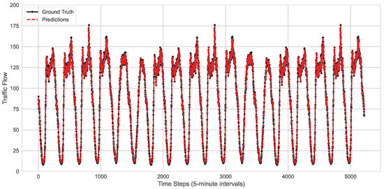
Figure 3.
The performance of the model at node 58 of the PeMS03 dataset.
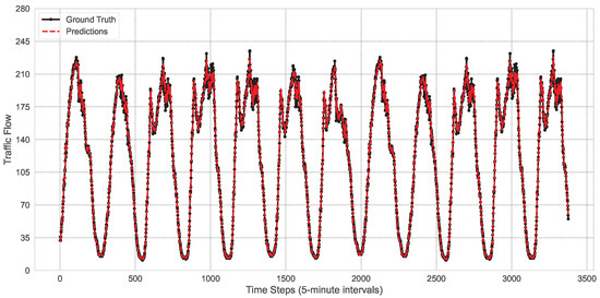
Figure 4.
The performance of the model at node 172 of the PeMS04 dataset.
5.2. Dynamic Scaling Experiment of Microservices
5.2.1. System Configuration
This experiment further enhances the dynamic characteristics of request volume and nodes within the cluster. Microservice instances are deployed in an environment with dynamically changing nodes to minimize the global request latency. The experiment generates 5 applications in total, covering 10 different microservices, and the dependency relationships between microservices are modeled as an N-ary tree structure. For dynamic request scenarios, different arrival rate models are used to configure the parameters of user requests for microservices, and the request data is generated based on three distribution patterns: Poisson distribution, long-tailed distribution, and exponential distribution. Meanwhile, multiple time points are randomly selected from the above three distribution patterns to inject a large number of request flows, simulating burst traffic scenarios.
is defined as the critical load threshold for performance degradation of MEC servers. When the load exceeds this value, resource contention leads to a non-linear decline in effective computing capacity. Combined with the resource model in Section 3.3.2, and integrating the M/M/S queuing model with stress test data (when simulating IoV requests, a CPU utilization rate of 70–80% causes a sharp increase in latency), is set to 0.7. The MGPPO adjustment cycle is set to 5 min, which is consistent with the time granularity of traffic flow prediction and matches the typical deployment time of container instances (approximately 2–3 min), ensuring that pre-allocated resources take effect in a timely manner. The triggering condition for FLA is set as , which is based on the stability criterion of the M/M/S queue model: when the request arrival rate exceeds the average service rate, the queue length will continue to grow, so this is used as the standard to trigger the rapid expansion mechanism.
5.2.2. Baselines and Metrics
To evaluate the effectiveness of the proposed STGT model, we compare it with several classical and state-of-the-art methods for traffic flow prediction:
- (1)
- DDQN [28]: A reinforcement learning method based on the Double Deep Q-Network, designed for dynamic service deployment scenarios. It improves resource utilization, service deployment success rate, and response efficiency by incorporating experience replay and target network mechanisms.
- (2)
- A3C-R2N2 [32]: A task scheduling strategy that combines the R2N2 with the A3C algorithm. It is suitable for cloud-edge collaborative environments and capable of handling complex temporal dependencies and dynamic resource allocation.
- (3)
- GA-MSP [34]: A microservice deployment approach based on an improved non-dominated sorting genetic algorithm. Targeted at mobile edge computing scenarios, it aims to reduce service chain transmission latency and improve server load balancing.
- (4)
- HPA [17]: The Kubernetes-native Horizontal Pod Autoscaler adjusts the number of service instances dynamically based on resource usage metrics such as CPU and memory, making it suitable for applications with significant workload fluctuations.
5.2.3. Results
Figure 5 illustrates the relationship between the number of system instances and the number of requests under three request distribution models. It can be observed that if the difference in the number of requests is small, the agent tends to take no action and maintain the original state of the system after comprehensively considering the scaling cost and queuing delay. From the overall trend, the greater the number of requests, the more instances there are, and the number of instances stops increasing once the resource limit is reached; the fewer the number of requests, the fewer instances there are.
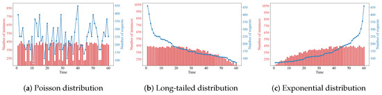
Figure 5.
Changes in the number of system instances.
Figure 6 illustrates the relationship between the average request latency of the system and the number of requests under three request distribution models. Analysis shows that when the number of requests increases within a certain range, the average latency fluctuates within a certain range, which indicates that MGPPO can suppress the increase in overall request latency by increasing microservice instances. If the number of requests is excessively large, the system has insufficient resources for expansion, leading to an increase in the number of queued requests, and thus the average request latency will increase accordingly.
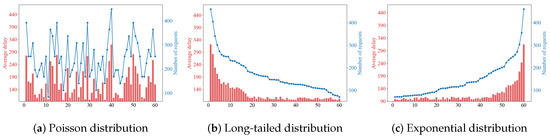
Figure 6.
Changes of average delay.
Figure 7 illustrates the relationship between system resource consumption and the number of requests under three request distribution models. Analysis shows that as the number of requests increases, MGPPO increases the number of deployed instances, thereby increasing resource consumption; conversely, as the number of requests decreases, MGPPO reduces the number of deployed instances, leading to decreased resource consumption. When the number of requests exceeds a certain threshold, MGPPO has consumed all resources in the cluster, and resource consumption no longer increases.
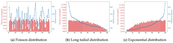
Figure 7.
Changes of resource consumption.
Figure 8 presents a performance comparison between the proposed MGPPO algorithm and two baseline algorithms: DDQN and A3C-R2N2. As shown in the figure, all three algorithms exhibit a gradual increase in reward values with more training iterations, eventually stabilizing over time. However, the MGPPO algorithm demonstrates a significantly faster convergence speed, reaching a higher reward level at an earlier stage. This indicates that MGPPO achieves higher sample efficiency and more stable learning performance during the reinforcement learning policy update process. In contrast, the DDQN and A3C-R2N2 algorithms perform relatively worse in terms of both policy convergence speed and reward stability—particularly showing larger fluctuations during the early learning phase. These results highlight the advantages of MGPPO in handling complex decision-making tasks related to microservice scheduling and scaling in vehicular networks.
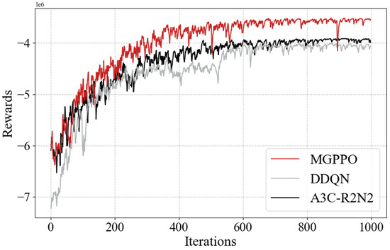
Figure 8.
The MGPPO algorithm.
As shown in Figure 9, the ablation study comparing the proposed MGPPO algorithm with the original PPO algorithm demonstrates that the mask mechanism and graph embedding strategy introduced in MGPPO play a crucial role in improving algorithmic performance. By comparing the reward curves of the two algorithms, it can be observed that MGPPO exhibits a faster and more stable upward trend from the early stages of training and maintains a higher level of reward throughout the entire training process. In contrast, the original PPO algorithm shows notable fluctuations and lower stability.
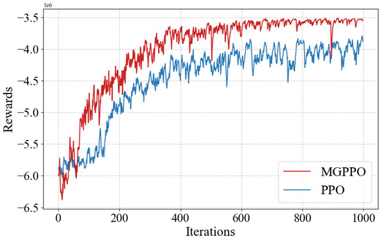
Figure 9.
Ablation study of MGPP.
This indicates that the mask mechanism in MGPPO effectively reduces the action space, thereby lowering the exploration difficulty in high-dimensional and complex state spaces. Meanwhile, the graph embedding strategy successfully captures the topological relationships among MEC edge nodes, leading to significantly improved generalization capability and decision-making quality of the algorithm.
Figure 10 and Figure 11 present five repeated experiments in which varying numbers of requests were added over the same time period after static deployment. The performance of MGPPO, DDQN, and A3C-R2N2 was compared in terms of request latency and resource utilization.
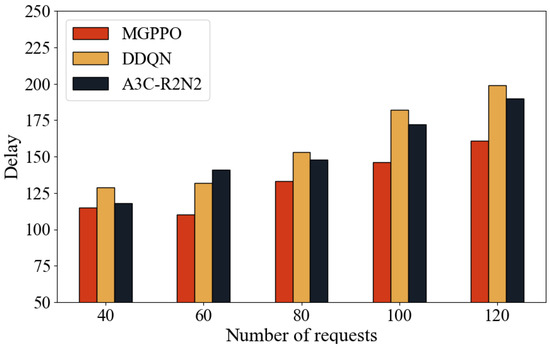
Figure 10.
Delay Performance under varying request loads.
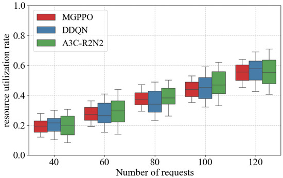
Figure 11.
Resource utilization performance under varying request loads.
As shown in Figure 10, when the number of requests increases within a moderate range, all three algorithms can effectively suppress latency growth through timely scaling, with MGPPO showing the best performance. Under sufficient resource conditions, MGPPO nearly eliminates latency increases. However, as system load becomes heavier due to increased request volume, latency rises for all methods despite instance scaling—mainly due to queue buildup. Thanks to its ability to model node topologies, MGPPO achieves better scaling placement decisions, reducing latency increases by more than 25% on average compared to baseline algorithms. Moreover, as the number of microservice types grows, MGPPO maintains stable performance, while DDQN and A3C-R2N2 show significantly higher latency increases, indicating their limited adaptability in complex scenarios.
As shown in Figure 11, resource utilization improves with increasing request volume for all algorithms. When the request count is 40, the median resource utilizations are approximately 0.20 (MGPPO), 0.22 (DDQN), and 0.19 (A3C-R2N2). At 120 requests, these values rise to about 0.55, 0.57, and 0.54, respectively. From the distribution perspective, MGPPO exhibits smaller interquartile ranges across all request levels, indicating lower variability and greater stability in resource allocation. This makes MGPPO better suited for dynamic vehicular environments with fluctuating workloads, leading to improved overall resource efficiency and service quality.
To evaluate the performance of the FLA, this experiment compares it with the heuristic algorithm GA-MSP and Kubernetes’ native HPA algorithm. FLA is designed to trade off some degree of global optimality for faster response times. Since HPA cannot perform real-time monitoring like FLA and GA-MSP, a random monitoring interval between 10 and 20 s is introduced in the simulation—based on HPA’s typical 15 s sampling cycle in real systems—to better mimic its behavior.
Figure 12 and Figure 13 show that FLA achieves the lowest latency across all test scenarios under varying request loads. As the number of requests increases, the performance of all algorithms degrades, but FLA remains superior. Compared to HPA, FLA reduces response time by approximately 80–90%, and average request latency by about 20–30%. Compared to GA-MSP, FLA reduces response time by 50–70%, and average request latency by 10–15%.
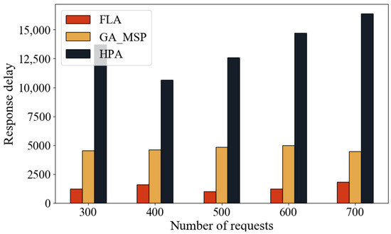
Figure 12.
Response latency.
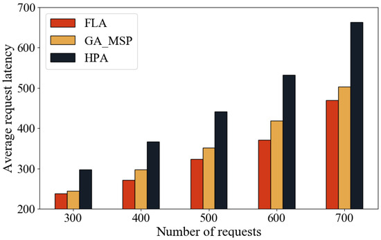
Figure 13.
Average request latency.
This advantage stems from the FLA’s ability to make resource scaling decisions based on real-time queueing information. In contrast, HPA is limited by fixed sampling intervals and cannot adapt quickly to dynamic load changes, while GA-MSP, although effective in dynamic environments, suffers from high computational overhead. Therefore, FLA demonstrates stronger adaptability and responsiveness in highly dynamic environments, making it well-suited for latency-sensitive applications such as vehicular networks.
The experimental results preliminarily confirm the effectiveness of the proposed two-stage dynamic scaling mechanism, but its practical deployment performance still requires further exploration in conjunction with the characteristics of vehicular edge computing environments.
The core design of this mechanism aligns well with practical requirements: The STGT model captures the spatiotemporal dependencies of traffic flow through a dynamic graph structure and self-attention mechanism, adapting to the spatiotemporal variations in traffic volume; the MGPPO algorithm integrates a graph convolutional network to model service dependencies and optimize resource allocation for coordinated multi-service operations; and the FLA algorithm, based on the M/M/S queuing model, enables rapid response to burst traffic, meeting the high-concurrency and low-latency demands of edge environments.
However, limitations exist in practical deployment: First, STGT relies on high-quality traffic data, and its prediction accuracy may degrade in areas with sparse sensors or unstable data transmission. Second, the training and inference processes of MGPPO consume computational resources, potentially increasing computational latency on edge nodes with limited hardware capabilities. Third, the rapid scaling of FLA depends on fast container startup/shutdown and image pulling; network bandwidth fluctuations in edge environments could lead to delays in container initialization, affecting the responsiveness to burst traffic.
5.3. Algorithm Real-Time Feasibility Analysis
Training time is a core metric for measuring computational complexity during the model development phase. As shown in the left bar chart of Figure 14, under an experimental environment equipped with an NVIDIA GeForce RTX 3090 GPU and Intel Core i9-13900KF CPU and built on the PyTorch 1.10.0 framework, the STGT model requires approximately 12 h for training, while the MGPPO model takes about 18 h to complete training. This significant time difference indicates that MGPPO consumes more computational resources and time during the training process. From an algorithmic logic perspective, MGPPO involves more complex state-space exploration and policy optimization mechanisms, leading to higher computational overhead during iterative training; in contrast, the training process of STGT is more streamlined and efficient.
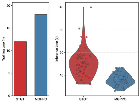
Figure 14.
Comparative analysis of training and inference times for STGT and MGPPO.
The inference time directly determines the real-time performance of models in practical application scenarios. The violin plot on the right side of Figure 14 illustrates the time distribution characteristics of 60 inference runs each for STGT and MGPPO (the experimental environment remains consistent with the training phase, using the RTX 3090 GPU, i9-13900KF CPU, and executed on the PyTorch 1.10.0 framework). The results show that STGT’s inference time is primarily concentrated within the 5 to 20 s range, although there is some variability, with certain samples approaching 40 s. In contrast, MGPPO’s inference time is stably concentrated between 5 and 12 s, exhibiting a more compact distribution. Although STGT’s inference time shows greater fluctuations, it maintains relatively fast response speeds in most cases, whereas MGPPO demonstrates stronger real-time processing capabilities due to its more stable inference times.
6. Conclusions
In this work, we have presented a dual-phase dynamic microservice scaling mechanism tailored to IoV edge computing environments, addressing the spatiotemporal variability and burstiness of user requests. Secondly, we have designed the STGT to predict long-term traffic trends, laying a foundation for proactive resource allocation. In addition, we have proposed an improved reinforcement learning algorithm, MGPPO, which integrates graph convolutional networks and dynamic masking mechanisms to optimize scaling decisions, and an FLA algorithm based on the M/M/S queuing model to handle short-term traffic surges. We use real datasets, PeMS03 and PeMS04, to compare the proposed mechanism with baseline algorithms such as DDQN, A3C-R2N2, GA-MSP, and Kubernetes HPA. The experimental results show that the STGT model outperforms existing methods in traffic prediction accuracy, with MAE reduced by up to 21.95%, and the combination of MGPPO and FLA outperforms baseline algorithms in request latency reduction by more than 25% on average, as well as resource utilization stability. Even under dynamically changing request intensities, the proposed mechanism maintains excellent performance, demonstrating its broad effectiveness and adaptability in complex IoV edge environments.
Author Contributions
Conceptualization, Y.J. and Z.W.; methodology, Y.J.; software, Z.Y. and G.D.; validation, G.D.; investigation, X.H.; resources, C.Z. and Z.W.; data curation, J.H.; writing—original draft preparation, Z.Y. and J.H.; writing—review and editing, J.L. and C.Z. All authors have read and agreed to the published version of the manuscript.
Funding
This research was funded in part by the Key Research and Development Program of Hubei Province, China, under Grants 2024BAA011, 2024BAB031, and 2024BAB016.
Data Availability Statement
Data are available on request from the authors.
Conflicts of Interest
The authors declare no conflicts of interest.
References
- Yang, F.; Wang, S.; Li, J.; Liu, Z.; Sun, Q. An overview of internet of vehicles. China Commun. 2014, 11, 1–15. [Google Scholar] [CrossRef]
- Ji, B.; Zhang, X.; Mumtaz, S.; Han, C.; Li, C.; Wen, H.; Wang, D. Survey on the internet of vehicles: Network architectures and applications. IEEE Commun. Stand. Mag. 2020, 4, 34–41. [Google Scholar] [CrossRef]
- Taslimasa, H.; Dadkhah, S.; Neto, E.C.P.; Xiong, P.; Ray, S.; Ghorbani, A.A. Security issues in Internet of Vehicles (IoV): A comprehensive survey. Internet Things 2023, 22, 100809. [Google Scholar] [CrossRef]
- Cao, K.; Liu, Y.; Meng, G.; Sun, Q. An overview on edge computing research. IEEE Access 2020, 8, 85714–85728. [Google Scholar] [CrossRef]
- Kong, L.; Tan, J.; Huang, J.; Chen, G.; Wang, S.; Jin, X.; Zeng, P.; Khan, M.; Das, S.K. Edge-computing-driven internet of things: A survey. ACM Comput. Surv. 2022, 55, 174. [Google Scholar] [CrossRef]
- Sharma, M.; Tomar, A.; Hazra, A. Edge computing for industry 5.0: Fundamental, applications, and research challenges. IEEE Internet Things J. 2024, 11, 19070–19093. [Google Scholar] [CrossRef]
- Peng, K.; Wang, L.; He, J.; Cai, C.; Hu, M. Joint optimization of service deployment and request routing for microservices in mobile edge computing. IEEE Trans. Serv. Comput. 2024, 17, 1016–1028. [Google Scholar] [CrossRef]
- Peng, K.; He, J.; Guo, J.; Liu, Y.; He, J.; Liu, W.; Hu, M. Delay-aware optimization of fine-grained microservice deployment and routing in edge via reinforcement learning. IEEE Trans. Netw. Sci. Eng. 2024, 11, 6024–6037. [Google Scholar] [CrossRef]
- Xu, B.; Guo, J.; Ma, F.; Hu, M.; Liu, W.; Peng, K. On the joint design of microservice deployment and routing in cloud data centers. J. Grid Comput. 2024, 22, 42. [Google Scholar] [CrossRef]
- Hu, M.; Guo, Z.; Wen, H.; Wang, Z.; Xu, B.; Xu, J.; Peng, K. Collaborative Deployment and Routing of Industrial Microservices in Smart Factories. IEEE Trans. Ind. Inform. 2024, 20, 12758–12770. [Google Scholar] [CrossRef]
- Kephart, J.; Chess, D. The vision of autonomic computing. Computer 2003, 36, 41–50. [Google Scholar] [CrossRef]
- Herbst, N.R.; Kounev, S.; Reussner, R. Elasticity in Cloud Computing: What it is, and What it is Not. In Proceedings of the 10th International Conference on Autonomic Computing (ICAC 2013), San Jose, CA, USA, 26–28 June 2013. [Google Scholar]
- Verma, A.; Pedrosa, L.; Korupolu, M.; Oppenheimer, D.; Tune, E.; Wilkes, J. Large-scale cluster management at Google with Borg. In Proceedings of the Tenth European Conference on Computer Systems, Bordeaux, France, 21–24 April 2015; pp. 1–17. [Google Scholar]
- Medel, V.; Tolosana-Calasanz, R.; Ángel Bañares, J.; Arronategui, U.; Rana, O.F. Characterising resource management performance in Kubernetes. Comput. Electr. Eng. 2018, 68, 286–297. [Google Scholar] [CrossRef]
- Zhou, S.; Wei, C.; Song, C.; Pan, X.; Chang, W.; Yang, L. Short-Term Traffic Flow Prediction of the Smart City Using 5G Internet of Vehicles Based on Edge Computing. IEEE Trans. Intell. Transp. Syst. 2023, 24, 2229–2238. [Google Scholar] [CrossRef]
- Pham, Q.V.; Fang, F.; Ha, V.N.; Piran, M.J.; Le, M.; Le, L.B.; Hwang, W.J.; Ding, Z. A Survey of Multi-Access Edge Computing in 5G and Beyond: Fundamentals, Technology Integration, and State-of-the-Art. IEEE Access 2020, 8, 116974–117017. [Google Scholar] [CrossRef]
- Toka, L.; Dobreff, G.; Fodor, B.; Sonkoly, B. Machine Learning-Based Scaling Management for Kubernetes Edge Clusters. IEEE Trans. Netw. Serv. Manag. 2021, 18, 958–972. [Google Scholar] [CrossRef]
- Chen, L.; Bai, Y.; Zhou, P.; Li, Y.; Qu, Z.; Xu, J. On Adaptive Edge Microservice Placement: A Reinforcement Learning Approach Endowed With Graph Comprehension. IEEE Trans. Mob. Comput. 2024, 23, 11144–11158. [Google Scholar] [CrossRef]
- Hochreiter, S.; Schmidhuber, J. Long Short-Term Memory. Neural Comput. 1997, 9, 1735–1780. [Google Scholar] [CrossRef]
- Wang, T.; Xue, S.; Yang, G.; Gao, S.; Ouyang, M.; Chen, L. Research on Traffic Flow Prediction and Traffic Light Timing Recommendation Technology Based on Vehicle Data Analysis. In Proceedings of the CCF Conference on Computer Supported Cooperative Work and Social Computing, Harbin, China, 18–20 August 2023; pp. 536–546. [Google Scholar]
- Li, Y.; Yu, R.; Shahabi, C.; Liu, Y. Diffusion convolutional recurrent neural network: Data-driven traffic forecasting. arXiv 2017, arXiv:1707.01926. [Google Scholar]
- Zhao, Y.; Luo, X.; Ju, W.; Chen, C.; Hua, X.S.; Zhang, M. Dynamic Hypergraph Structure Learning for Traffic Flow Forecasting. In Proceedings of the 2023 IEEE 39th International Conference on Data Engineering (ICDE), Anaheim, CA, USA, 3–7 April 2023; pp. 2303–2316. [Google Scholar] [CrossRef]
- Yu, B.; Yin, H.; Zhu, Z. Spatio-temporal graph convolutional networks: A deep learning framework for traffic forecasting. arXiv 2017, arXiv:1709.04875. [Google Scholar]
- Bai, L.; Yao, L.; Kanhere, S.; Wang, X.; Sheng, Q. Stg2seq: Spatial-temporal graph to sequence model for multi-step passenger demand forecasting. arXiv 2019, arXiv:1905.10069. [Google Scholar]
- Wu, Z.; Pan, S.; Long, G.; Jiang, J.; Zhang, C. Graph wavenet for deep spatial-temporal graph modeling. arXiv 2019, arXiv:1906.00121. [Google Scholar]
- Li, D.C.; Huang, C.T.; Tseng, C.W.; Chou, L.D. Fuzzy-based microservice resource management platform for edge computing in the internet of things. Sensors 2021, 21, 3800. [Google Scholar] [CrossRef]
- Zarie, M.M.; Ateya, A.A.; Sayed, M.S.; ElAffendi, M.; Abdellatif, M.M. Microservice-Based Vehicular Network for Seamless and Ultra-Reliable Communications of Connected Vehicles. Future Internet 2024, 16, 257. [Google Scholar] [CrossRef]
- Zhao, Y.; Wang, J.; Li, B. A deep reinforcement learning approach to online microservice deployment in mobile edge computing. In Proceedings of the International Conference on Service-Oriented Computing, Rome, Italy, 28 November–1 December 2023; pp. 127–142. [Google Scholar]
- Santos, J.; Wauters, T.; Volckaert, B.; De Turck, F. gym-hpa: Efficient auto-scaling via reinforcement learning for complex microservice-based applications in kubernetes. In Proceedings of the NOMS 2023—2023 IEEE/IFIP Network Operations and Management Symposium, Miami, FL, USA, 8–12 May 2023; pp. 1–9. [Google Scholar]
- Samanta, A.; Tang, J. Dyme: Dynamic microservice scheduling in edge computing enabled IoT. IEEE Internet Things J. 2020, 7, 6164–6174. [Google Scholar] [CrossRef]
- Wang, S.; Ding, Z.; Jiang, C. Elastic scheduling for microservice applications in clouds. IEEE Trans. Parallel Distrib. Syst. 2020, 32, 98–115. [Google Scholar] [CrossRef]
- Tuli, S.; Ilager, S.; Ramamohanarao, K.; Buyya, R. Dynamic Scheduling for Stochastic Edge-Cloud Computing Environments Using A3C Learning and Residual Recurrent Neural Networks. IEEE Trans. Mob. Comput. 2022, 21, 940–954. [Google Scholar] [CrossRef]
- Rossi, F.; Cardellini, V.; Presti, F.L.; Nardelli, M. Dynamic multi-metric thresholds for scaling applications using reinforcement learning. IEEE Trans. Cloud Comput. 2022, 11, 1807–1821. [Google Scholar] [CrossRef]
- Li, H.; Tang, B.; Xu, W.; Guo, F.; Zhang, X. Application Deployment in Mobile Edge Computing Environment Based on Microservice Chain. In Proceedings of the 2022 IEEE 25th International Conference on Computer Supported Cooperative Work in Design (CSCWD), Hangzhou, China, 4–6 May 2022; pp. 531–536. [Google Scholar] [CrossRef]
- Shifrin, M.; Mitrany, R.; Biton, E.; Gurewitz, O. VM Scaling and Load Balancing via Cost Optimal MDP Solution. arXiv 2016, arXiv:1611.06956. [Google Scholar] [CrossRef]
- Garg, D.; Narendra, N.C.; Tesfatsion, S. Heuristic and reinforcement learning algorithms for dynamic service placement on mobile edge cloud. arXiv 2021, arXiv:2111.00240. [Google Scholar] [CrossRef]
- Chen, C.; Petty, K.; Skabardonis, A.; Varaiya, P.; Jia, Z. Freeway performance measurement system: Mining loop detector data. Transp. Res. Rec. 2001, 1748, 96–102. [Google Scholar] [CrossRef]
- Wang, X. PeMS03 and PeMS04. IEEE Dataport, 8 October 2024. [Google Scholar] [CrossRef]
Disclaimer/Publisher’s Note: The statements, opinions and data contained in all publications are solely those of the individual author(s) and contributor(s) and not of MDPI and/or the editor(s). MDPI and/or the editor(s) disclaim responsibility for any injury to people or property resulting from any ideas, methods, instructions or products referred to in the content. |
© 2025 by the authors. Licensee MDPI, Basel, Switzerland. This article is an open access article distributed under the terms and conditions of the Creative Commons Attribution (CC BY) license (https://creativecommons.org/licenses/by/4.0/).