Abstract
The recommendation system based on graphs aims to infer the symmetrical relationship between unconnected users and items nodes. Graph convolutional neural networks (GCNs) are powerful deep learning models widely used in recommender systems, showcasing outstanding performance. However, existing GCN-based recommendation models still suffer from the well-known issue of over-smoothing, which remains a significant obstacle to improve the recommendation performance. Additionally, traditional neighborhood aggregation methods of GCN-based recommendation models do not differentiate the nodes’ importance and also exert a certain negative impact on the recommendation effect of the model. To address these problems, we first propose a simple yet efficient GCN-based recommendation model, named WR-GCN, with a node-based dynamic weighting method and a flexible residual strategy. WR-GCN can effectively alleviate the over-smoothing issue and utilize the interaction information among the graph nodes, enhancing the recommendation performance. Furthermore, building upon the outstanding performance of contrastive learning (CL) in recommendation systems and its robust capability to address data sparsity issues, we integrate the proposed WR-GCN into a simple CL framework to form a more potent recommendation model, WR-GCL, which incorporates an initial embedding controlling method to strike a balanced state of high-frequency information. We have conducted extensive experiments on the proposed WR-GCN and WR-GCL models on multiple datasets. The experimental results show that WR-GCN and WR-GCL outperform several state-of-the-art baselines.
1. Introduction
In recent years, recommendation models based on graph convolutional neural networks (GCNs) have made great success in improving recommending performance [1,2,3,4,5]. This success can be attributed to the powerful capabilities of GCNs in handling graph data. In recommendation systems, interaction data inherently manifest graph structures [6,7].
Scholars have extensively studied the recommendation model based on the GCN, resulting in a substantial enhancement in performance [8,9,10,11,12,13,14,15]. NGCF [11] has exploited high-order connectivity through integrating multiple layers of embedded propagation, facilitating representation learning for inactive users. However, certain operations within GCN models, such as non-linear activation and feature transformation, do not yield a positive impact on recommendation performance. Instead, they may introduce additional computational complexity and resource overhead [11]. To tackle these issues, researchers have proposed simplified GCN models for recommendation [8,9,10,12]. For instance, LR_GCCF [12] eliminates non-linear activation functions from GCNs and computes final embeddings through a residual connection. LightGCN [10] removes non-linear activation functions and feature transformation modules from GCNs, retaining only neighborhood aggregation for feature updates and propagation. LightGCN demonstrates outstanding computational power and recommendation effectiveness in the recommendation system, with a simple structure, and is easily expandable. Although LR_GCCF and LightGCN partially alleviate over-smoothing, it is not particularly significant. IMP-GCN [9] introduces a subgraph generation module to alleviate the negative impact of high-order neighbor nodes, leading to improved performance. LayerGCN [8] focuses on the process of node-embedding learning and information propagation and refines the hidden layer during this process. Additionally, LayerGCN employs an alternative approach of degree-sensitive pruning and probability pruning to sparsify the user-item interaction graph, aiming to improve recommendation performance.
However, there are two issues with these aforementioned models. Firstly, like other graph neural networks, these models face the challenge of over-smoothing as the number of convolutional layers increases. This poses a dilemma in GCN-based recommendation models, as enhancing recommendation performance requires the stacking of more convolutional layers to aggregate more neighborhood information. Secondly, in these GCN-based recommendation models, the convolution layer assigns equal importance to each node, thereby significantly impacting performance enhancement.
Additionally, to address the sparsity problem within recommendation system, researchers have applied contrastive learning (CL) to recommendation systems [16,17,18,19,20,21]. To improve the accuracy and robustness of GCNs for recommendation, SGL [16] generates multiple different views through graph augmentations and then constructs a self-supervised learning task based on CL. Subsequently, Yu et al. [22] reveal that graph augmentations do not significantly improve performance and proposed a simple contrastive learning method called SimGCL, which constructs contrastive views in a way that mixes uniform noises in the embedding. Moreover, building upon SimGL, they have integrated the primary recommendation task with the auxiliary comparison learning task and proposed a simplified CL recommendation method XSimGCL [23]. Additionally, NCL [24] considers the structural and semantic neighbors of users or items as contrastive targets. However, the aforementioned CL-based recommendation models all rely on LightGCN as the primary component of the GCL framework. Consequently, they still suffer from the issue of over-smoothing.
To address the aforementioned issues, we explore a novel CL-based recommendation model via differential weighting GCN model with a flexible residuals strategy. Firstly, we propose a simpler and more efficient GCN-based recommendation model with differential weights and a flexible residuals strategy. We name this model as WR-GCN. Specifically, based on LightGCN, we allocate different weights to each node according to the similarity of node embeddings between adjacent convolutional layers during the linear propagation process. Furthermore, we introduce a residual strategy that uses a parameter to control from which layer the residual modules are added. We further integrate WR-GCN into a simple contrastive learning framework, which is named as WR-GCL, improving the training efficiency and recommendation performance. The main contributions of our work are as follows.
- We investigate the existing recommendation models based on GCNs and propose a flexible residual connection strategy, which effectively alleviates the over-smoothing issue in recommendation models based on GCNs.
- We propose a novel method named differential weighted aggregation for recommendation models based on GCNs. In contrast to conventional GCN-based recommendation models that perform graph convolution with uniform weight, the differential weighted aggregation identifies the importance of each node based on the similarity of embedding vectors across adjacent layers, enabling nodes to propagate in a linear manner. This method further improves the recommendation performance.
- Based on the aforementioned design, we propose an improved GCN-based recommendation model called WR-GCN. Subsequently, we integrate WR-GCN into a simple contrastive learning framework, where an initial embedding control method is utilized to achieve a balanced state of high-frequency information in the contrastive learning model, thereby further enhancing the recommendation performance of the model. We refer to this CL-based recommendation model as WR-GCL.
- We initially conducted experiments with WR-GCN on the Gowalla, Yelp2018, and Amazon-Book datasets. The experimental results demonstrate that the WR-GCN outperforms baselines models, particularly in deeper convolution layers. Subsequently, experiments were performed on the WR-GCL model using the Douban-Book, Yelp2018, and Amazon-Book datasets, with the results indicating that the WR-GCL outperforms existing models.
2. Related Work
In this section, we begin by reviewing recent advancements in recommendation models based on GCNs. Subsequently, we introduce the CL-based methods and models relevant to the field of recommendation. These studies serve as inspiration for the design of our model.
2.1. Recommendation Models Based on GCNs
With the proliferation of various media tools, recommendation systems have permeated various aspects of people’s lives [25]. The advancement of graph theory techniques [26,27] and graph neural networks [28,29] has established a solid theoretical and technical foundation for graph structure-based recommendation systems. In particular, in recent years, GCN-based recommendation models have achieved significant success in enhancing performance. By iteratively applying convolutional layers, GCNs effectively aggregate feature information from the multi-order neighborhood [30], enabling powerful representation learning from non-Euclidean structures. Since Thomas N. Kipf et al. [30] first utilized GCNs to process graph-structured data, various recommendation models based on GCNs have been developed, achieving significant improvement in performance [8,9,10,11,12].
Recent studies have shown that the non-linear activation and feature transformation modules within GCNs do not necessarily improve recommendation performance [10]. Observing this insight, LR_GCCF [12] has removed the non-linear operator from GCNs, and connects embeddings from each layer, obtaining the final embedding representation. Similarly, LightGCN [10] completely discarded non-linear activation and feature transformation, retaining only the basic neighborhood aggregation operator. Essentially, LightGCN presents itself as a simpler and more scalable graph convolutional model, as evidenced by exprimental results showcasing its excellent computational efficiency and performance in recommendation systems. However, neither LR_GCCF nor LightGCN effectively alleviated the over-smoothing issue inherent in GCN. Recognizing the significance of high-order neighbors of user nodes in embedding learning, IMP-GCN [9] devised a subgraph generation module to mitigate the negative impact of high-order neighbor nodes. LayerGCN [8] concentrated on embedding learning and refining hidden layers during information propagation processes. Furthermore, to sparsify the user-item interaction graph, LayerGCN adopted a method involving alternately performing degree-sensitive pruning and probability pruning, thus achieving better recommendation performance.
It should be noted that our proposed WR-GCN model differs significantly from similar models, such as lightGCN [10] and LR_GCCF [12]. Firstly, while WR-GCN, like lightGCN and LR_GCCF, employs a normalized sum aggregation during the process of linear information propagation in each convolutional layer, it also considers the differences in nodes through the cosine similarity of the adjacent node’s embedding. Secondly, LR_GCCF incorporates residual connections for user preference prediction, while WR-GCN applies a residual connection strategy in GCN information propagation.
2.2. Recommendation Models Based on Graph Contrastive Learning
In recent years, research on contrastive learning has continuously risen and made significant progress in multiple fields [16,31,32,33]. Recognizing the powerful capability of CL in addressing the sparsity issue in recommendation systems [34], more and more researchers have applied CL to existing recommendation models, resulting in significant performance improvements [16,17,18,19,20,21]. In 2021, Wu et al. [16] proposed a model named SGL, which generates multiple different views through data augmentation on the graph, such as edge dropout, node dropout, and random walk. It then maximizes the difference between representations of different nodes through contrastive learning. SGL greatly enhanced recommendation performance and provided a new perspective for subsequent research. Following SGL, researchers have proposed a series of CL-based recommendation models [22,23,24]. For example, SimGCL [22] delved into the SGL model and other related CL-based recommendation models, concluding that the performance of recommendation is primarily determined by the CL loss rather than graph augmentation. These authors further proposed a graphless augmentation CL recommendation method based on noise perturbation and demonstrated effectiveness of the proposed SimGCL through extensive experiments. Building on SimGCL, the authors later introduced a structurally simpler CL recommendation method named XSimGCL [23]. XSimGCL integrates the primary recommendation task with the auxiliary contrastive learning task, further simplifying the model structure, significantly reducing computational costs, and improving recommendation performance. Additionally, starting from the neighborhood relations of interaction graphs, the NCL [24] model considers the structural neighbors and semantic neighbors of users or items as contrastive targets to compute the contrastive loss. Experimental results have demonstrated the effectiveness of NCL in recommendation performance.
However, the aforementioned CL-based recommendation models all rely on LightGCN as the graph encoder within constrastive learning framework. Consequently, these models remain susceptible to the over-smoothing issue, which hinders the enhancement of recommendation performance through the addition of more convolutional layers. In comparison with SimGCL [22], the primary task encoder of WR-GCL incorporates our proposed WR-GCN. Furthermore, in order to achieve a balanced representation of high-frequency information in the contrastive learning model, we investigate the extent to which the initial embedding contributes to the computation of final the embedding. This design, based on our findings, further enhances the model’s recommendation performance.
3. Methodology
In this section, we initially present the detailed design of WR-GCN. Then, we elaborate on its design principles and relevant mathematical formulations. Subsequently, we design a more robust graph contrastive recommendation model, WR-GCL, which integrates the WR-GCN.
3.1. WR-GCN
3.1.1. Overview of WR-GCN
In the following, we present a detailed description of the proposed WR-GCN model. WR-GCN distinguishes itself from current GCN-based models through three characteristics. (1) Differential weighting neighborhood aggregation: in WR-GCN, we dynamically adjust the weight of node features by utilizing the similarity of embedding vectors of adjacent layer nodes during the model’s propagation process. (2) Flexible residual connection strategy: WR-GCN introduces a parameter that controls the starting layer of the residual connection. This strategy enables the model to delve into deeper levels of convolution, aggregating a wider range of neighborhood information. (3) Layer combination and prediction: WR-GCN sums the embedding results of all layer and then average them to make prediction and recommendation.
As shown in Figure 1, the WR-GCN framework consists of three modules: input module, propagation module, and prediction module. The WR-GCN takes a bipartite graph of user and item interactions as input. In the propagation module, unlike the simple neighborhood aggregation in LightGCN, our proposed model computes the similarity of embedding vectors of adjacent layer nodes and incorporates the processed results as weights for the current layer’s linear propagation process. The W-module shown in Figure 1b implements this function. There are L layers in the propagation module. When the layer number is less than , every layer includes two W-Modules as shown in Figure 1b. One W-Module is for the feature extractor of users, and the other is for the feature extractor of items. Additionally, we apply a residual connections strategy to alleviate the over-smoothing issue, improving the representation and learning ability of the model. Specifically, when the layer number equals or is larger than , every layer includes two RW-Modules, as shown in Figure 1c. It should be noted that the W-Module or RW-Module used for user embedding extracting adopts a normalized sum block, as shown in Figure 1e, while the W-Module or RW-Module used for item embedding extracting adopts the normalized sum block shown in Figure 1d. Finally, we sum and average the embedding results obtained at each layer during the model’s propagation. Thus, we obtain two final embeddings that are used to calculate the prediction score.
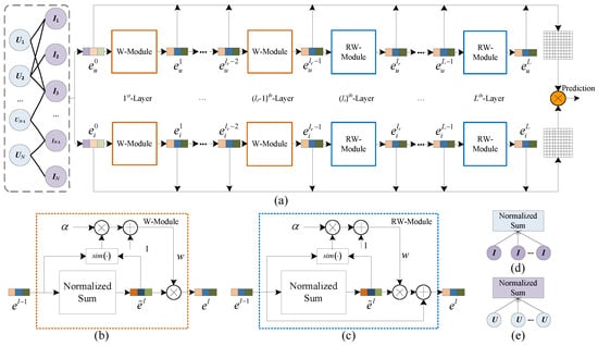
Figure 1.
The architecture of WR-GCN. (a) Architecture of WR-GCN. (b)W-Modules. (c) RW-Modules. (d) Aggregation of user nodes. (e) Aggregation of item nodes.
3.1.2. Differential Weighting Neighborhood Aggregation
In traditional GCN-based recommendation models, the aggregation methods in the graph convolution operation assign the same weight to each neighboring node. However, these methods neglect the differences among individual nodes, resulting in increased noise that degrades recommendation performance. Inspired by layerGCN [9], we propose a neighborhood aggregation method with differential weight. The key to this approach is to dynamically adjust the weights according to the similarity of embedding vectors between two adjacent layers’ nodes during graph information propagation. We design a W-Module, shown in Figure 1b, to implement a differential weighting neighborhood aggregation method. The detailed procedures of the W-Module are as follows.
(1) Normalize sum aggregation. Like LightGCN, WR-GCN adopts a simple neighborhood aggregation. Let and denote the node embeddings of users and items at the l-th layer in the graph convolution operation, respectively. The aggregation in WR-GCN is defined as
where is the item node set interacting with user u, and is the user node set interacting with item i. The symmetric normalization term helps avoid the scale of embeddings increasing with graph convolution operations.
(2) Dynamically adjust weight. Firstly, we calculate the cosine similarity of nodes between adjacent graph convolution layers. The calculation of cosine similarity is as follows:
Secondly, to mitigate model over-fitting, we introduce a shrinkage factor , which is applied as a multiplier to the cosine similarity, and then added to the original weight of 1 to derive the final weights. The calculating of weights can be formulated as
where is a contraction factor whose function is to scale the cosine similarity between node embeddings. Since the is changed according to the embedding of nodes in the propagation process, we can dynamically adjust the weight for each node in the current layer.
(3) Graph convolution operator. Once we obtain the weights of the nodes, we formulate the output of the l-th layer of WR-GCN as
where is the learnable weights matrix, is the Sigmoid activation function. Here, denotes the normalized adjacency matrix, which can be expressed by
Here, we denote the W-Module as , where is the learning parameters.
Our model dynamically conducts feature learning based on the node-specific design of differential weighting neighborhood aggregation, thereby enhancing model flexibility and reducing the generation and impact of noise during model propagation. As a result, our design can to some extent improve recommendation performance. The effectiveness of WR-GCN will be demonstrated in Section 4.
3.1.3. Flexible Residual Connection Strategy
To further alleviate the performance degradation problem caused by over-smoothing, we attempt to integrate a residual strategy into the WR-GCN model. Unlike the traditional residuals method for the GCN, we introduce a parameter to specify the layer from which the residual module is incorporated. We refer to this residual module as the RW-Module, as illustrated in Figure 1c.
Specifically, when the layer number is less then , WR-GCN utilizes W-Modules; otherwise, it employs RW-Modules. Compared to the W-Module, a residual connection is simply added from the embedding of previous node to the output of the RW-Module. In other words, we enable the network block W-Module to learn the residual features. The output of the RW-Module in the l-th layer can be expressed as follows.
where represents the previous node’s embedding. We let denote the RW-Module, where is the learning parameters. By introducing residual connections, the model’s training gradient vanishing problem can be alleviated, making it easier for the model to learn more information in deep convolutions [35]. Additionally, residual connections preserve more low-order embedding information during the convolution process. To some extent, our residual strategy mitigates the over-smoothing issue caused by an increase in convolutional layers. In the next section, we will analyze the impact of different residual connection strategies on model performance and conduct experiments to determine specific strategies.
Finally, we sum the embedding presentation of all layers and then calculate the average. Specifically, the output of the WR-GCN model can be expressed as follows:
So far, the algorithm of WR-GCN can be described as Algorithm 1. The complexity of Algorithm 1 is , where is the number of edges in the user-item bipartite graph, d is the embedding dimension, and L is the number of layers. After analysis, the complexity of WR-GCN is consistent with that of LightGCN.
| Algorithm 1 Algorithm of WR-GCN |
|
3.1.4. Loss Function of WR-GCN
To train the WR-GCN model, we adopt pairwise Bayesian Personalized Ranking (BPR) [36] as the loss function. Specifically, the loss function is expressed as
where is the user representation, B is a mini-batch, is the sigmoid function, is the representation of a random sample item, and is the representation of an item that user u has interacted with.
3.1.5. Analysis
Similar to other graph neural networks, GCNs suffer from the over-smoothing issue as the number of network layers increases. Residual techniques represent one of the effective approaches to mitigate the over-smoothing problem in graph neural networks [37]. Mathematically, the residual connection of the l-th in the GCN can be formally expressed as follows [35]:
where denotes the output of the preceding layer, and is a hyperparameter that serves as a weight coefficient for controlling the proportion of residual mapping in the current layer. represents the neural network of the layer, and is the parameters of neural layer. If we reorganize Formulas (1)–(6), we obtain the following formula.
where . Here, represents Equation (1), and is Equation (2). After analysis, it was found that Equations (9) and (10) have the same expression. Therefore, we think our method also can effectively mitigate the issue of over-smoothing. It should be noted that in Equation (9), the parameter is a hyperparameter with fixed value, while the weight coefficient in Equation (10) is a dynamic weight that adjusts according to the input embedding representation and hyperparameter . Consequently, WR-GCN can be regarded as a novel approach to implementing weighted residual connections for addressing the over-smoothing issue.
3.2. WR-GCL
In this subsection, we explore the integration of our proposed model, WR-GCN, into a contrastive learning framework to enhance recommendation performance.
3.2.1. Overview of WR-GCL
In recent years, some researchers leveraged the advancements in contrastive learning to GCN-based recommendation models. Several studies [16,22,23,24] have utilized LightGCN [10] as the graph encoder in their contrastive learning-based recommendation models. However, it has been observed that the performance of LightGCN tends to deteriorate when the number of convolutional layer exceeds three, primarily due to the over-smoothing issue inherent in GCNs. Motivated by this observation, we sought to investigate the potential for improved recommendation performance by integrating our proposed WR-GCN model into contrastive learning. Consequently, we incorporate the WR-GCN model into a simplified contrastive learning framework, resulting in a novel contrastive recommendation model, WR-GCL. The architecture of the WR-GCL model is illustrated in Figure 2. Extensive experiments are conducted in Section 4 to thoroughly validate its effectiveness in recommendation performance.
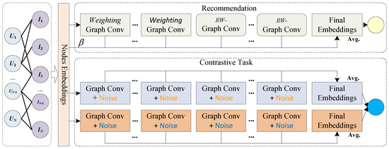
Figure 2.
Architecture of WR-GCL.
3.2.2. Contrastive Learning Model Design Based on WR-GCN
To effectively integrate WR-GCN into contrastive learning, we employ the simple yet efficient contrastive recommendation model SimGCL [22] as the main framework. In WR-GCL, we adopt a similar architecture to that of SimGCL. As shown in Figure 2, WR-GCL consists of three graph encoders. For contrastive tasks, we utilize the same graph encoder as SimGCL. It is worth noting that these graph encoders incorporate added noise perturbations to augment the node representation. The perturbations in noise for the embeddings of the i-th node can be expressed by [22]
where the added noise vector and are subject to and , . Here, is a small constant. The final embedding of contrastive tasks is expressed by
where L is the number of layers in the graph contrastive task.
In the primary recommendation task, WR-GCL utilizes the WR-GCN model as the graph encoder. To improve the performance of recommendation, a control strategy for initial embeddings has been developed in the WR-GCL model. Specifically, we introduce a hyperparameter to control the proportion of initial embedding involved in the computation of final embedding . Further elaboration on this strategy is provided in the subsequent subsection.
Subsequently, in WR-GCL, we adopt Equation (13) as the joint loss function. The first term of Equation (13) is the standard BPR loss as WR-GCN. The second term is the InfoNCE loss [38] for contrastive learning.
where e represents the final embeddings obtained by applying WR-GCN to the primary recommendation task, is a hyperparameter, and is a hyperparameter. and denote the final embedding results obtained from the other two graph encoders in the contrastive learning task. The algorithm for WR-GCL is presented in Algorithm 2. The complexity of Algorithm 2 is , which is three times that of WR-GCN because there is one primary task and two contrastive tasks in WR-GCL.
| Algorithm 2 Algorithm for WR-GCL. |
|
3.2.3. Tradeoff Design of Initial Embedding for WR-GCL
Some studies revealed that the incorporating initial embeddings can alleviate the over-smoothing issue to some extent in GCN-based recommendation models and enable the model to capture more extensive neighborhood information [10,39]. On the other hand, in the SimGCL framework, if the initial embedding is involved in the calculation of final representation, it deviates from the graph augmentation criterion; i.e., the difference in high-frequency parts is greater than the difference in low-frequency parts, thereby adversely affecting the effectiveness of graph contrastive learning [22,23,40].
Based on the theoretical support and analysis mentioned above, we believe that it is essential to find a balance point that can effectively alleviate the over-smoothing issue without compromising the effectiveness of contrastive learning. Within the WR-GCL framework, we incorporate only the initial embedding to the main recommendation task and associate the -graph convolutional layers with . In the -graph convolutional layers, a hyper parameter is introduced to regulate , thereby preventing an excessive amount of high-frequency information in the final embedding representation. Specifically, the formula for calculating the final embedding can be expressed as
Here, we use fine-tuning to determine the optimal value of hyperparameter within the range . Experiments validate the effectiveness of WR-GCL in Section 4.4.2.
4. Experiment and Results
We carry out extensive experiments on benchmark datasets to assess the WR-GCN and WR-GCL models. Our aim is to address the following research questions:
- RQ1: Can WR-GCN significantly alleviate the over-smoothing issue and achieve good performance in recommendation tasks? (Section 4.3.2)
- RQ2: Is the combination of WR-GCN with contrastive learning models still effective? (Section 4.4.2)
- RQ3: What is the effect of introducing different residual connections during the propagation process? (Section 4.3.4)
- RQ4: What impact do individual components of the model have on overall performance? (Section 4.3.3 and Section 4.4.3)
- RQ5: Is the influence of hyperparameters on model performance significant? What selection of hyperparameters can achieve relatively optimal results? (Section 4.3.4 and Section 4.4.4)
4.1. Datasets
In this subsection, we provide a unified description of the four datasets used in our experiments. The datasets include Gowalla [41], Amazon-Book [42], Yelp2018 [11], and Douban-Book [43]. The detailed information of these datasets are presented in Table 1. The Gowalla dataset comprises user check-in records collected from the Gowalla application on smartphones. The Amazon-Book dataset, provided by Amazon, consists of book review data from its users. The Yelp2018 dataset originates from the Yelp challenge held in the United States in 2018, encompassing business record data from millions of enterprises such as bars and restaurants. The Douban-Book dataset is sourced from online book rating data on the Douban website. The WR-GCN experiments were conducted on the Gowalla, Yelp2018, and Amazon-Book datasets, while the WR-GCL experiments were performed on the Douban-Book, Yelp2018, and Amazon-Book datasets.

Table 1.
Datasets description.
4.2. Evaluation Metrics
Our proposed WR-GCN and WR-GCL models are implemented by using the Python 3.6 language. The training and testing of the WR-GCN and WR-GCL models were conducted on a DELL server, which was equipped with an Intel Xeon Bronze 3106 CPU @ 1.70 GHz, an Nvidia GeForce 2080Ti GPU, 96 GB of DDR4 memory, and Ubuntu 20.04 operating system. To observe and validate the performance of the two models more intuitively, we employ recall calculated over top-K items (Recall@K) and normalized discounted cumulative gain over top-K items (NDCG@K) as evaluation metrics. In all experiments, we set .
4.3. Experiment and Results of WR-GCN
4.3.1. Experimental Setup
In this subsection, we first introduce the baseline models in comparison with the WR-GCN model and then present the parameter settings used in the experiments.
We compare WR-GCN with several baseline recommendation models as follows.
- LightGCN [10] is a GCN-based recommendation model that removes non-linear activations and feature transformations from GCNs, achieving better recommendation performance with a light weight structure.
- DGCF [13] is a GCN-based collaborative filtering model that models from the perspective of user intentions, obtaining finer-grained embedding representations and significantly enhancing the recommendation effectiveness of the model.
- UltraGCN [14] is a GCN model for recommendation systems that bypasses infinite-layer explicit message passing, achieving more efficient recommendation performance.
- IA-GCN [15] is a GCN-based recommendation model that utilizes the aggregated interactions of users and items to guide node aggregation during the embedding process, resulting in superior recommendation performance.
In this experiment, we select the Gowalla, Yelp2018, and Amazon-Book datasets, which were randomly allocated in a ratio of 0.8, 0.1, 0.1 for training, validation, and testing sets, respectively. In the experiment, we set the regularization coefficient to 1 × , the size of the embedding layer to 64, the learning rate to 0.001, and the training epochs to 1000. To enhance training speed, we set the batch sizes for Gowalla, Yelp2018, and Amazon-Book to 2048, 8192, and 2048, respectively. Additionally, we progressively increase the number of convolutional layers in the WR-GCN model to evaluate the impact of the over-smoothing issue on model performance.
4.3.2. Performance Comparison
Firstly, we compare WR-GCN with several other GCN-based baselines. As shown in the experimental results in Table 2, WR-GCN outperforms the baselines models on the Gowalla and Yelp2018 datasets. Moreover, WR-GCN achieved notably better performance on the Amazon dataset, although it falls short of UltraGCN’s performance. These results validate the effectiveness of our proposed approach for the WR-GCN model.
Table 2.
Performance comparison among GCN-based baseline models on three datasets.
Secondly, we evaluate the ability of WR-GCN to alleviate over-smoothing by comparing it with LightGCN under different layers. The performance comparison is shown in Table 3. From the table, we can discern two significant observations. Firstly, at every layer, WR-GCN outperforms LightGCN on three datasets. Under eight layers of convolution, in the Gowalla dataset, recall increased by 12.17%, and NDCG increased by 11.54%. In the Amazon-Book dataset, recall increased by 26.69%, and NDCG increased by 27.18%. In the Yelp2018 dataset, recall increased by 13.33%, and NDCG increased by 14.17%. These results validate the effectiveness of WR-GCN in recommendation performance. Secondly, LightGCN achieves its best performance at the third or fourth layer. However, as the number of graph convolutional layers increase, the performance of LightGCN decreases. In contrast, the performance of WR-GCN continually increases until reaching the eighth layer. This experiment demonstrates that WR-GCN’s capacity to alleviate over-smoothing surpasses that of LightGCN.
Table 3.
Performance comparison between LightGCN and WR-GCN across different layers.
Thirdly, Figure 3 presents the comparison of performance curves between WR-GCN and LightGCN across different epochs during the training phase. These curves indicate that WR-GCN outperforms LightGCN on all metrics at each epoch. As the number of epoch reaches 1000, the performance across all metrics stabilizes.
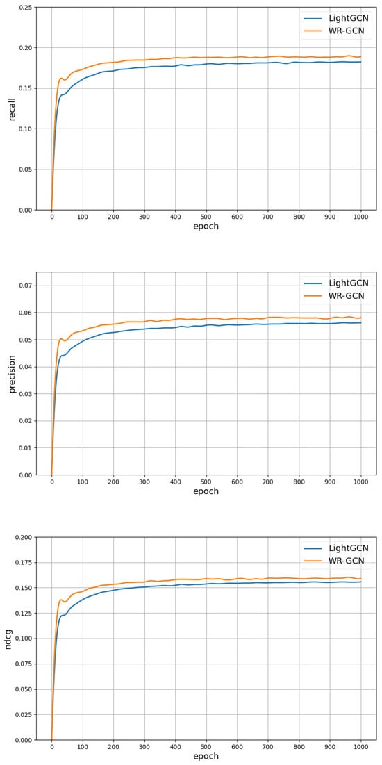
Figure 3.
Performance comparison between WR-GCN and LightGCN on three evaluation metrics across different epochs.
Finally, Table 4 presents a comparison between the WR-GCN and LightGCN models, including training time, parameter size, and Flops. Taking the Gowalla dataset as an example, it can be observed from Table 4 that the parameter size of WR-GCN is identical to that of LightGCN when both models employ four convolutional layers, but the training time and Flops of WR-GCN are both larger than those of LightGCN. Due to the ability of WR-GCN to alleviate the issue of over smoothing, it enables the network convolutional layers to be deepened, for example, reaching up to eight layers. Simultaneously, this also resulted in a significant increase in computational resource requirements. Therefore, as shown in Table 4, the eight-layer WR-GCN model has witnessed significant improvements in terms of training time, parameter size, and FLOPS. The other two datasets also share similar characteristics with Gowalla. The reason for this lies in the calculation of Equation (3), which incorporates the cosine similarity operator.
Table 4.
Model comparison between WR-GCN and LightGCN.
4.3.3. Ablation Analysis
We analyzed different variants of WR-GCN to explore the contributions of various improvement strategies. In this subsection, we set up two variants of WR-GCN as follows:
WR-GCN-or: A variant only includes the residual connection strategy. Specifically, when the layer number is less than , WR-GCN-or employs the normalized sum module, named the NS-Module, as shown in Figure 1d or Figure 1e, during linear propagation. Starting from the -th layer, WR-GCN-or utilizes the NS-Module as the residual module.
WR-GCN-ow: A variant only includes differential weight neighborhood aggregation. We compute the cosine similarity between each layer’s convolutional embedding and its previous layer’s embedding, then multiply this value by a contraction factor as an added weight and fuse it with the original embedding.
We conduct ablation experiments between the aforementioned two variants and WR-GCN on the Gowalla, Yelp2018, and Amazon-Book datasets. From the experimental results shown in Table 5, we can observe that WR-GCN-or outperforms WR-GCN-ow on all three datasets. The reason is that WR-GCN-or can incorporate more information from neighbor nodes through a deeper network model compared to WR-GCN-ow. On the other hand, WR-GCN achieves the best recommendation performance among all variants. These observations validate the effectiveness of our design that combines differential weighting neighborhood aggregation and flexible residual network structure. Furthermore, in comparison to LightGCN, we can observe a significant performance enhancement in WR-GCN. For instance, In the Amazon-Book dataset, the recall metric increased from 0.04110 for LightGCN to 0.04336 for WR-GCN-or, representing a significant improvement of 5.49%. Similarly, the NDCG metric increased from 0.03150 for LightGCN to 0.03376 for WR-GCN-or, representing a significant improvement of 7.17%. Obviously, the reason is that WR-GCN-or incorporates our proposed residual connection strategy.
Table 5.
Performance comparison among ablation GCN models on three databases.
4.3.4. Analysis of Hyperparameters
We investigate the impact of two related hyperparameters: the number of graph convolution layers L and the residual connections starting from the -th layer. Experimental results and analysis are as follows:
The effect of L on WR-GCN. As shown in Table 3, the performance of WR-GCN gradually increases with the increase in the graph convolution layer. When the number of layers reaches eight, the performance of WR-GCN is optimal. However, the performance of LightGCN continued to deteriorate starting from three layers. On the Yelp2018 dataset, a similar trend also occurs when the layer number starts from five. This demonstrates that our proposed method can effectively mitigate the over-smoothing issue in GNNs and can be stacked with deeper layers to enhance performance.
The effect of -th on WR-GCN. The weight coefficient calculated by Equation (3) is incorporated into the GCN graph convolution operation, as shown in Equation (4). If , it is the same as the standard GCN model. To retain most of the features and to reflect the feature differences before and after node graph convolution, we need close to 1.0. Furthermore, Equation (2) gives out the formula of cosine similarity, whose value falls in . Therefore, the hyperparameter is preferably around 0.1. Additionally, Section 4.4.4 will discuss the effect of on WR-GCL. The results of the experiment on hyperparameter demonstrates that WR-GCL achieved the best performance when .
The effect of -th on WR-GCN. In WR-GCN, we introduce residual connections starting from the -th layer rather than incorporating them across all convolutional layers. To verify the validity of our approach, we design a series models, denoted as WR-GCN_all, according to the number of layers. In WR-GCN_all, all models only adopt residual connections across all convolutional layers. Experiments are conducted on the Gowalla, Yelp2018, and Amazon-Book datasets. Figure 4 illustrates the performance comparison between WR-GCNs and WR-GCN_alls with different layers, ranging from three to eight layers.
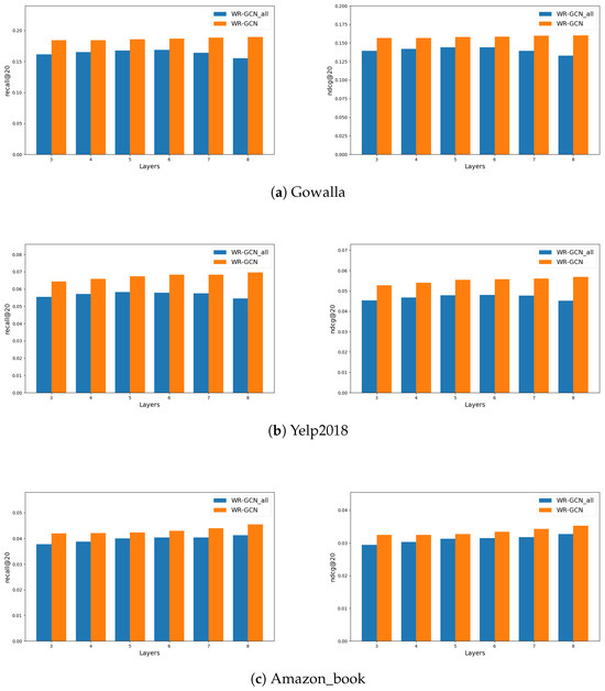
Figure 4.
Performance comparison between WR-GCN and WR-GCN_all with residual connection across different layers.
Experimental results demonstrate that WR-GCNs consistently outperform WR-GCN_alls at different layers. Generally speaking, GCN-based recommendation models require two to three graph convolutional layers to aggregate sufficient useful information. However, WR-GCN_all excessively concentrates information on the insights gained from low-order convolutions. This potentially leads to the model learning excessive noise and consequently decreasing performance. Furthermore, excessive residual connections may result in gradient explosion, leading to over-fitting during model training and only achieving suboptimal performance. Therefore, in WR-GCN, flexibly controlling is a useful strategy to design residual structures. This approach can effectively alleviate the over-smoothing issue in GCN models and achieves superior recommendation performance.
4.4. Experiment and Results of WR-GCL
4.4.1. Experimental Setup
In this subsection, we first introduce the baseline models in comparison with the WR-GCL model and then present the parameters settings used in the experiments.
We compare WR-GCL with several baseline recommendation models, as briefly outlined below.
- Mult-VAE [44] is a collaborative filtering model based on variational autoencoder with a reconstruction objective, enabling better capturing of latent representations of users and items using autoencoders.
- LightGCN [10] is a GCN-based recommendation model that removes non-linear activations and feature transformations from GCNs, achieving better recommendation performance with a lightweight structure.
- MixGCF [45] is an approach to training GNN recommendation system models using mixed negative sampling, greatly enhancing the recommendation performance of the model.
- DNN+SSL [46] is a recommendation method using the DNN as the graph encoder, employing feature masking and feature dropout through contrastive learning.
- SimGCL [22] is a recommendation model based on graph contrastive learning, demonstrating the non-necessity of graph augmentation in graph contrastive learning and acquiring different contrastive views through uniform noise perturbation.
To evaluate the performance of WR-GCL, we conduct comparison experiments with baseline models on the Douban-Book, Yelp2018, and Amazon-Book datasets. In the experiments, we allocate these three datasets into training, validation, and testing sets in the ratio of 7:1:2. Regarding parameter settings, we also set the regularization parameter value to 1 × , the size of the embedding layer to 64, the learning rate to 0.001, and the batch size to 2048. For the Douban-Book, Yelp2018, and Amazon-Book datasets, we set the number of epochs to 50, 100, and 30, respectively. Additionally, due to dataset-specific hyperparameters in the model, different values were assigned for various datasets. The detailed parameter settings are presented in Table 6.
Table 6.
Parameter settings for different dataset.
4.4.2. Performance Comparison
The performance comparison between WR-GCL and baseline models is shown in Table 7. From the data in Table 7, it can be observed that WR-GCL significantly outperforms the other competing baselines on all three datasets. The significant improvement in performance of WR-GCL can be attributed to three factors. Firstly, the W-Module or RW-Module blocks in WR-GCN assign different weights to each node, according to the similarity between embeddings of the previous and current layers during the propagation process. This design helps to distinguish the importance of the nodes and contributes to improvement of recommendation performance in WR-GCL. Secondly, as graph encoder, WR-GCN employs a flexible residual design that retains more information from lower-order embeddings, deepens the network layer, and captures more neighbor information through graph convolution. This flexible residual design is of great significance for alleviating the over-smoothing issue. Thirdly, WR-GCL enables partial initial embedding involved in the expression of the final embedding. This design alleviates the adverse effects on contrastive learning and enables the model to learn more extensive neighborhood information.
Table 7.
Performance comparison among baseline models on three datasets.
To further intuitively observe the impact of WR-GCL in alleviating the issue of over-smoothing, we conduct a comparison of recommendation performance with SimGCL across different convolutional layers, ranging from two to six layers. Table 8 presents the comparison of performance. It can be seen that on the three experimental datasets, the performance of SimGCL tends to stabilize at the second convolutional layer. However, increasing the number of convolutional layers does not bring greater performance improvement. On the contrary, our proposed WR-GCL exhibits noticeable performance improvement up to the sixth layer. Intriguingly, a sudden decrease in performance is observed at the fourth convolutional layer on the Douban_book and Yelp2018 datasets. This phenomenon stems from the introduction of residual structures starting from the fourth layer, where the initial embedding is involved in the calculation of final embeddings. The addition of initial embeddings affects contrastive learning efficacy and subsequently impacts overall recommendation performance [22,23]. However, the performance enhancement due to alleviating over-smoothing at layer four is less pronounced in Douban_book and Yelp2018, contributing significantly to the observed performance degradation in these datasets. As WR-GCL progresses to deeper convolutional layers, performance swiftly recovers and reaches higher levels at layer 6. These experimental results validate the effectiveness of our proposed design.
Table 8.
Performance comparison between SimGCL and WR-GCL across different layers on three datasets.
4.4.3. Ablation Analysis
In this subsection, we set up four variants of WR-GCL to investigate the impact of each component on overall performance.
WR-GCL-or: A variant of WR-GCL that adopts WR-GCN-or as the graph encoder in the primary recommendation task. It should be noted that the initial embedding is involved in the calculation of the final embedding.
WR-GCL-ow: A variant of WR-GCL that adopts WR-GCN-ow model as the graph encoder in the primary recommendation task. And this variant does not uses the initial embedding to compute the final embedding.
WR-GCL-ore: A variant of WR-GCL that uses WR-GCN-or as the graph encoder in the primary recommendation task. Additionally, this variant uses the hyperparameter to control how much initial embedding is added to the final embedding.
WR-GCL-orw: A variant of WR-GCL that uses GCN, which only consists of the WR-Module as the graph encoder in the primary recommendation task. Here, the entire initial embedding participates in the calculation of the final embedding.
The performance comparison among the four variants with WR-GCL is shown in Table 9. Based on the data in Table 9, the following observations are drawn: Firstly, WR-GCL achieves the best overall performance on three experimental datasets. Secondly, the outstanding performance of WR-GCL-ow demonstrates the effectiveness of the differential weighting neighborhood aggregation in our design. Thirdly, compared to WR-GCL-or, WR-GCL-ore achieves better performance. This demonstrates that partial involvement of in the calculation of final embedding helps improve performance. Moreover, the network structure of WR-GCL is similar to that of WR-GCL-orw, except that is involved in the final embedded calculation, and it achieves the best recommendation performance. These results validate our previous analysis on how to add initial embeddings in contrastive learning, as discussed in Section 3.2.3. These ablation experiments indicate that WR-GCL can effectively mitigate the over-smoothing issue and enhance the recommendation performance.
Table 9.
Performance comparison among ablation GCL models on three databases.
4.4.4. Analysis of Hyperparameters
We investigate the impact of three related hyperparameters: the number of graph convolution layers L, the contraction factor , and the initial embedding ratio . Experimental results and analysis are as follows:
The effect of L on WR-GCL. As shown in Table 8, the overall performance of WR-GCL gradually increases with the increase in graph convolution layers of WR-GCN. The optimal performance is achieved in the sixth layer. This demonstrates that it will achieve the optimal performance by using WR-GCN stacked deeper graph convolution layers.
The influence of the on WR-GCL. In WR-GCN model, we set the parameter to 0.1 and obtain significant performance improvement. However, may not necessarily make the WR-GCL model achieve optimal recommendation performance. To further investigate the impact of the shrinkage factor on the WR-GCL model, we conducted parameter-tuning experiments within the range {0.05, 0.1, 0.2, 0.3, 0.5, 0.7, 1.0}. As depicted in Figure 5, the model achieves relatively optimal recommendation performance when is set to 0.1.
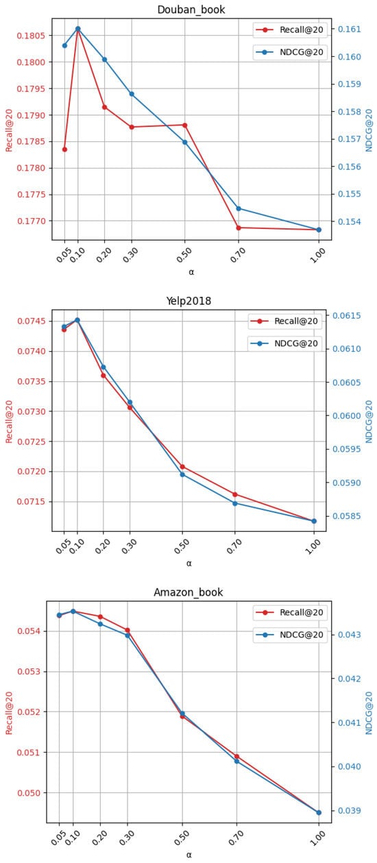
Figure 5.
The performance comparison of WR-GCL with varying values of the parameter .
The effect of the on WR-GCL. Experiments are conducted with . The experimental results are shown in Figure 6. From Figure 6, we can observe that the performance of WR-GCL is relatively better when approaches the middle value. On the contrary, when the value of is too small or too large, the model performance deteriorates. These experimental results further demonstrate that adding a certain proportion of to the final embedding can improve the performance of WR-GCL, as discussed in Section 3.2.3. In WR-GCL experiments, we set for the Douban-Book, Yelp2018, and Amazon-Book datasets to attain relatively optimal performance.
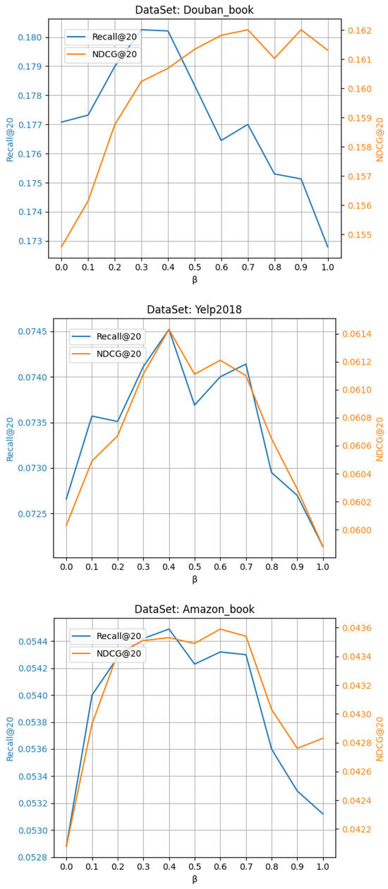
Figure 6.
The performance comparison of WR-GCL with varying values of the parameter .
5. Conclusions
In this paper, we first design WR-GCN, which effectively improves the over-smoothing issue through a flexible residual strategy. Furthermore, by investigating the similarity between embedding vectors in adjacent convolutional layers, dynamic weighting is applied during neighborhood aggregation, enhancing the recommendation performance of the model. Additionally, we integrate our proposed WR-GCN into a CL-based recommendation framework, which incorporates the initial embeddings controlling method to achieve a balanced state of high-frequency information, resulting in a superior recommendation model, WR-GCL. We conduct extensive experiments on several benchmark datasets to evaluate the performance of the WR-GCN and WR-GCL models. The experimental results demonstrate that our proposed models can attain superior recommendation performance compared to several SOTA baseline models.
Although the WR-GCN and WR-GCL models have demonstrated excellent performance on the experimental datasets, there is still room for improvement in our proposed models, which can be addressed as follows. Firstly, when the number of graph convolutional layers is large, the computing resources required by WR-GCN are relatively high. Secondly, further validation and application in real-world scenarios are still required. Therefore, future work will focus on optimizing and deploying the proposed methods in practical applications, such as drug–target interaction prediction, personalized recommendation systems, and so on.
Author Contributions
Conceptualization, M.W. and F.X.; methodology, M.W.; software, F.X.; validation, D.S., J.P. and F.X.; formal analysis, M.W.; investigation, M.W. and F.X.; resources, F.X.; data curation, F.X. and J.P.; writing—original draft preparation, F.X.; writing—review and editing, M.W., J.P. and D.S.; visualization, D.S. and J.P.; supervision, M.W.; project administration, M.W.; funding acquisition, M.W. All authors have read and agreed to the published version of the manuscript.
Funding
This research was funded by the National Natural Science Foundation of China under Grant 62362002.
Data Availability Statement
The codes of WR-GCN and WR-GCL are available at https://github.com/ThreeCathan/WRGCNandWRGCL.git (accessed on 10 August 2025).
Conflicts of Interest
The authors declare no conflicts of interest.
Abbreviations
The following abbreviations are used in this manuscript:
| GCN | Graph Convolutional Network |
| CL | Contrastive Learning |
| WR-GCN | GCN model with differential weights and flexible residuals strategy |
| GCL | Graph Contrastive Learning |
| WR-GCL | GCL model integrating WR-GCN |
References
- Wang, X.; Zhang, Z.; Shen, G.; Lai, S.; Chen, Y.; Zhu, S. Multi-view knowledge graph convolutional networks for recommendation. Appl. Soft Comput. 2025, 169, 112633. [Google Scholar] [CrossRef]
- Duan, Y.; Zhang, L.; Lu, X.; Li, J. Light Graph Convolutional Recommendation Algorithm Based on Hybrid Spreading. Appl. Sci. 2025, 15, 1898. [Google Scholar] [CrossRef]
- Su, Y.; Wei, P.; Zhu, L.; Xu, L.; Wang, X.; Tong, H.; Han, Z. Lbgcn: Lightweight bilinear graph convolutional network with attention mechanism for recommendation. Appl. Intell. 2025, 55, 465. [Google Scholar] [CrossRef]
- Jiang, M.; Li, M.; Cao, W.; Yang, M.; Zhou, L. Multi-task convolutional deep neural network for recommendation based on knowledge graphs. Neurocomputing 2025, 619, 129136. [Google Scholar] [CrossRef]
- Hassanzadeh, R.; Majidnezhad, V.; Arasteh, B. A novel recommender system using light graph convolutional network and personalized knowledge-aware attention sub-network. Sci. Rep. 2025, 15, 15693. [Google Scholar] [CrossRef] [PubMed]
- Berg, R.v.d.; Kipf, T.N.; Welling, M. Graph convolutional matrix completion. arXiv 2017, arXiv:1706.02263. [Google Scholar] [CrossRef]
- Ying, R.; He, R.; Chen, K.; Eksombatchai, P.; Hamilton, W.L.; Leskovec, J. Graph convolutional neural networks for web-scale recommender systems. In Proceedings of the 24th ACM SIGKDD International Conference on Knowledge Discovery & Data Mining, London, UK, 19–23 August 2018; pp. 974–983. [Google Scholar]
- Zhou, X.; Lin, D.; Liu, Y.; Miao, C. Layer-refined graph convolutional networks for recommendation. In Proceedings of the 2023 IEEE 39th International Conference on Data Engineering (ICDE), Anaheim, CA, USA, 3–7 April 2023; pp. 1247–1259. [Google Scholar]
- Liu, F.; Cheng, Z.; Zhu, L.; Gao, Z.; Nie, L. Interest-aware message-passing GCN for recommendation. In Proceedings of the Web Conference 2021, Ljubljana, Slovenia, 19–23 April 2021; pp. 1296–1305. [Google Scholar]
- He, X.; Deng, K.; Wang, X.; Li, Y.; Zhang, Y.; Wang, M. Lightgcn: Simplifying and powering graph convolution network for recommendation. In Proceedings of the 43rd International ACM SIGIR Conference on Research and Development in Information Retrieval, Virtual, 25–30 July 2020; pp. 639–648. [Google Scholar]
- Wang, X.; He, X.; Wang, M.; Feng, F.; Chua, T.S. Neural Graph Collaborative Filtering. In Proceedings of the SIGIR’19: 42nd International ACM SIGIR Conference on Research and Development in Information Retrieval, Paris, France, 21–25 July 2019; ACM: New York, NY, USA, 2019; pp. 165–174. [Google Scholar] [CrossRef]
- Chen, L.; Wu, L.; Hong, R.; Zhang, K.; Wang, M. Revisiting graph based collaborative filtering: A linear residual graph convolutional network approach. In Proceedings of the AAAI Conference on Artificial Intelligence, New York, NY, USA, 7–12 February 2020; Volume 34, pp. 27–34. [Google Scholar]
- Wang, X.; Jin, H.; Zhang, A.; He, X.; Xu, T.; Chua, T.S. Disentangled graph collaborative filtering. In Proceedings of the 43rd International ACM SIGIR Conference on Research and Development in Information Retrieval, Virtual, 25–30 July 2020; pp. 1001–1010. [Google Scholar]
- Mao, K.; Zhu, J.; Xiao, X.; Lu, B.; Wang, Z.; He, X. UltraGCN: Ultra simplification of graph convolutional networks for recommendation. In Proceedings of the 30th ACM International Conference on Information & Knowledge Management, Virtual, 1–5 November 2021; pp. 1253–1262. [Google Scholar]
- Zhang, Y.; Wang, P.; Zhao, X.; Qi, H.; He, J.; Jin, J.; Peng, C.; Lin, Z.; Shao, J. IA-GCN: Interactive graph convolutional network for recommendation. arXiv 2022, arXiv:2204.03827. [Google Scholar] [CrossRef]
- Wu, J.; Wang, X.; Feng, F.; He, X.; Chen, L.; Lian, J.; Xie, X. Self-supervised graph learning for recommendation. In Proceedings of the 44th International ACM SIGIR Conference on Research and Development in Information Retrieval, Virtual, 11 July 2021; pp. 726–735. [Google Scholar]
- Xia, X.; Yin, H.; Yu, J.; Wang, Q.; Cui, L.; Zhang, X. Self-supervised hypergraph convolutional networks for session-based recommendation. In Proceedings of the AAAI Conference on Artificial Intelligence, Virtual, 19–21 May 2021; Volume 35, pp. 4503–4511. [Google Scholar]
- Yu, J.; Yin, H.; Gao, M.; Xia, X.; Zhang, X.; Viet Hung, N.Q. Socially-aware self-supervised tri-training for recommendation. In Proceedings of the 27th ACM SIGKDD Conference on Knowledge Discovery & Data Mining, Virtual, 14–18 August 2021; pp. 2084–2092. [Google Scholar]
- Yu, J.; Yin, H.; Li, J.; Wang, Q.; Hung, N.Q.V.; Zhang, X. Self-supervised multi-channel hypergraph convolutional network for social recommendation. In Proceedings of the Web Conference 2021, Ljubljana, Slovenia, 19–23 April 2021; pp. 413–424. [Google Scholar]
- Zhou, C.; Ma, J.; Zhang, J.; Zhou, J.; Yang, H. Contrastive learning for debiased candidate generation in large-scale recommender systems. In Proceedings of the 27th ACM SIGKDD Conference on Knowledge Discovery & Data Mining, Virtual, 14–18 August 2021; pp. 3985–3995. [Google Scholar]
- Zhou, K.; Wang, H.; Zhao, W.X.; Zhu, Y.; Wang, S.; Zhang, F.; Wang, Z.; Wen, J.R. S3-rec: Self-supervised learning for sequential recommendation with mutual information maximization. In Proceedings of the 29th ACM International Conference on Information & Knowledge Management, Virtual, 19–23 October 2020; pp. 1893–1902. [Google Scholar]
- Yu, J.; Yin, H.; Xia, X.; Chen, T.; Cui, L.; Nguyen, Q.V.H. Are graph augmentations necessary? simple graph contrastive learning for recommendation. In Proceedings of the 45th International ACM SIGIR Conference on Research and Development in Information Retrieval, Madrid, Spain, 11–15 July 2022; pp. 1294–1303. [Google Scholar]
- Yu, J.; Xia, X.; Chen, T.; Cui, L.; Hung, N.Q.V.; Yin, H. XSimGCL: Towards extremely simple graph contrastive learning for recommendation. IEEE Trans. Knowl. Data Eng. 2023, 36, 913–926. [Google Scholar] [CrossRef]
- Lin, Z.; Tian, C.; Hou, Y.; Zhao, W.X. Improving graph collaborative filtering with neighborhood-enriched contrastive learning. In Proceedings of the ACM Web Conference 2022, Virtual, 25–29 April 2022; pp. 2320–2329. [Google Scholar]
- Wu, S.; Sun, F.; Zhang, W.; Xie, X.; Cui, B. Graph neural networks in recommender systems: A survey. ACM Comput. Surv. 2022, 55, 1–37. [Google Scholar] [CrossRef]
- Mahapatra, T.; Pal, M. An investigation on m-polar fuzzy threshold graph and its application on resource power controlling system. J. Ambient Intell. Humaniz. Comput. 2022, 13, 501–514. [Google Scholar] [CrossRef]
- Mahapatra, T.; Ghorai, G.; Pal, M. Competition graphs under interval-valued m-polar fuzzy environment and its application. Comput. Appl. Math. 2022, 41, 285. [Google Scholar] [CrossRef]
- Zhang, B.; Fan, C.; Liu, S.; Huang, K.; Zhao, X.; Huang, J.; Liu, Z. The Expressive Power of Graph Neural Networks: A Survey. IEEE Trans. Knowl. Data Eng. 2025, 37, 1455–1474. [Google Scholar] [CrossRef]
- Zhou, J.; Cui, G.; Hu, S.; Zhang, Z.; Yang, C.; Liu, Z.; Wang, L.; Li, C.; Sun, M. Graph neural networks: A review of methods and applications. AI Open 2020, 1, 57–81. [Google Scholar] [CrossRef]
- Kipf, T.N.; Welling, M. Semi-Supervised Classification with Graph Convolutional Networks. arXiv 2016. [Google Scholar] [CrossRef]
- Chen, T.; Kornblith, S.; Norouzi, M.; Hinton, G. A simple framework for contrastive learning of visual representations. In Proceedings of the International conference on Machine Learning, PMLR, Virtual, 13–18 July 2020; pp. 1597–1607. [Google Scholar]
- Gao, T.; Yao, X.; Chen, D. Simcse: Simple contrastive learning of sentence embeddings. arXiv 2021, arXiv:2104.08821. [Google Scholar]
- You, Y.; Chen, T.; Sui, Y.; Chen, T.; Wang, Z.; Shen, Y. Graph contrastive learning with augmentations. Adv. Neural Inf. Process. Syst. 2020, 33, 5812–5823. [Google Scholar]
- Hao, B.; Zhang, J.; Yin, H.; Li, C.; Chen, H. Pre-training graph neural networks for cold-start users and items representation. In Proceedings of the 14th ACM International Conference on Web Search and Data Mining, Virtual, 8–12 March 2021; pp. 265–273. [Google Scholar]
- Li, G.; Müller, M.; Thabet, A.; Ghanem, B. DeepGCNs: Can GCNs Go As Deep As CNNs? In Proceedings of the 2019 IEEE/CVF International Conference on Computer Vision (ICCV), Seoul, Republic of Korea, 27 October–2 November 2019; pp. 9266–9275. [Google Scholar] [CrossRef]
- Rendle, S.; Freudenthaler, C.; Gantner, Z.; Schmidt-Thieme, L. BPR: Bayesian personalized ranking from implicit feedback. In Proceedings of the Twenty-Fifth Conference on Uncertainty in Artificial Intelligence, Montreal, QC, Canada, 18–21 June 2009; UAI ’09. pp. 452–461. [Google Scholar]
- Rusch, T.K.; Bronstein, M.M.; Mishra, S. A Survey on Oversmoothing in Graph Neural Networks. arXiv 2023, arXiv:2303.10993. [Google Scholar] [CrossRef]
- van den Oord, A.; Li, Y.; Vinyals, O. Representation Learning with Contrastive Predictive Coding. arXiv 2018. [Google Scholar] [CrossRef]
- Gasteiger, J.; Bojchevski, A.; Günnemann, S. Predict then propagate: Graph neural networks meet personalized pagerank. arXiv 2018, arXiv:1810.05997. [Google Scholar]
- Liu, N.; Wang, X.; Bo, D.; Shi, C.; Pei, J. Revisiting graph contrastive learning from the perspective of graph spectrum. Adv. Neural Inf. Process. Syst. 2022, 35, 2972–2983. [Google Scholar]
- Cho, E.; Myers, S.A.; Leskovec, J. Friendship and mobility: User movement in location-based social networks. In Proceedings of the 17th ACM SIGKDD International Conference on Knowledge Discovery and Data Mining, San Diego, CA, USA, 21–24 August 2011; KDD ’11. pp. 1082–1090. [Google Scholar] [CrossRef]
- Ni, J.; Li, J.; McAuley, J. Justifying Recommendations using Distantly-Labeled Reviews and Fine-Grained Aspects. In Proceedings of the 2019 Conference on Empirical Methods in Natural Language Processing and the 9th International Joint Conference on Natural Language Processing (EMNLP-IJCNLP), Hong Kong, China, 3–7 November 2019; Inui, K., Jiang, J., Ng, V., Wan, X., Eds.; 2019; pp. 188–197. [Google Scholar] [CrossRef]
- Yin, H.; Cui, B.; Li, J.; Yao, J.; Chen, C. Challenging the long tail recommendation. Proc. VLDB Endow. 2012, 5, 896–907. [Google Scholar] [CrossRef]
- Liang, D.; Krishnan, R.G.; Hoffman, M.D.; Jebara, T. Variational autoencoders for collaborative filtering. In Proceedings of the 2018 World Wide Web Conference, Lyon, France, 23–27 April 2018; pp. 689–698. [Google Scholar]
- Huang, T.; Dong, Y.; Ding, M.; Yang, Z.; Feng, W.; Wang, X.; Tang, J. Mixgcf: An improved training method for graph neural network-based recommender systems. In Proceedings of the 27th ACM SIGKDD Conference on Knowledge Discovery & Data Mining, Virtual, 14–18 August 2021; pp. 665–674. [Google Scholar]
- Yao, T.; Yi, X.; Cheng, D.Z.; Yu, F.; Chen, T.; Menon, A.; Hong, L.; Chi, E.H.; Tjoa, S.; Kang, J.; et al. Self-supervised learning for large-scale item recommendations. In Proceedings of the 30th ACM International Conference on Information & Knowledge Management, Virtual, 1–5 November 2021; pp. 4321–4330. [Google Scholar]
Disclaimer/Publisher’s Note: The statements, opinions and data contained in all publications are solely those of the individual author(s) and contributor(s) and not of MDPI and/or the editor(s). MDPI and/or the editor(s) disclaim responsibility for any injury to people or property resulting from any ideas, methods, instructions or products referred to in the content. |
© 2025 by the authors. Licensee MDPI, Basel, Switzerland. This article is an open access article distributed under the terms and conditions of the Creative Commons Attribution (CC BY) license (https://creativecommons.org/licenses/by/4.0/).