Comparative Analysis of the Gardner Equation in Plasma Physics Using Analytical and Neural Network Methods

Abstract

In the present paper, a mathematical analysis of the Gardner equation with varying coefficients has been performed to give a more realistic model of physical phenomena, especially in regards to plasma physics. First, a Lie symmetry analysis was carried out, as a result of which a symmetry classification following the different representations of the variable coefficients was systematically derived. The reduced ordinary differential equation obtained is solved using the power-series method and solutions to the equation are represented graphically to give an idea of their dynamical behavior. Moreover, a fully connected neural network has been included as an efficient computation method to deal with the complexity of the reduced equation, by using traveling-wave transformation. The validity and correctness of the solutions provided by the neural networks have been rigorously tested and the solutions provided by the neural networks have been thoroughly compared with those generated by the Runge–Kutta method, which is a conventional and well-recognized numerical method. The impact of a variation in the loss function of different coefficients has also been discussed, and it has also been found that the dispersive coefficient affects the convergence rate of the loss contribution considerably compared to the other coefficients. The results of the current work can be used to improve knowledge on the nonlinear dynamics of waves in plasma physics. They also show how efficient it is to combine the approaches, which consists in the use of analytical and semi-analytical methods and methods based on neural networks, to solve nonlinear differential equations with variable coefficients of a complex nature.

1. Introduction

The investigation of the core principles that determine the behavior of gases, liquids, and plasmas comes under the study of fluid mechanics. In this subject, the forces that act on substances in motion and rest are taken into consideration. Plasma is commonly seen as the fourth state of matter, where there are freely moving charged particles, and their motion is greatly influenced by electromagnetic fields. As a result, plasma physics has become an important field of fluid mechanics, where the interaction of charged particles with a flow is investigated in the presence of external electromagnetic forces. The technologies of plasma modeling are applied to modeling many phenomena, such as magnetic confinement in fusion reactors, the dynamics of space plasma, and many areas in astrophysical and industrial processes [1]. Major functions in the scientific fields of accelerator physics, controlled fusion and beam storage technology, and astrophysics are overseen by plasma interactions. The mathematical representation of nonlinear phenomena intrinsic to both fluids and plasmas can be given in terms of nonlinear evolution equations (NLEEs). However, Korteweg–de Vries (KdV)-type equations can serve as effective models for long waves with small nonlinearities: ion acoustic waves, shallow-water waves, and acoustic waves in plasma and crystal lattices [2,3,4]. Mathematical descriptions of such phenomena contribute to the development of a high degree of knowledge concerning the actual physical processes taking part in them; and therefore are relevant to a wide variety of scientific work and industrial applications in the study of numerous phenomena. Additionally, some of the physical settings where mKdV-type equations have been found to be applicable are the quantum electron-acoustic waves in an electron–positron plasma; when Alfvén waves exist in a collisionless plasma; when interfacial waves arise in two layers of a liquid; when plasmon modes occur in a dusty plasma, and when optical pulses occur in Kerr-type nonlinear optical materials [5,6,7]. Together, the extended KdV (eKdV) is the combination of the properties of the KdV and mKdV equations; it is also known as the Gardner equation. It has been used to describe a range of nonlinear wave processes that appear in plasma physics, fluid dynamics, and nonlinear elasticity. In particular it has been applied to dust acoustic waves in dusty plasmas; internal waves in shear flows of oceans and the atmosphere; ion acoustic waves in plasmas with negative ions; surface water waves; and the flow of water in nonlinear elastic structures when large deflections occur [8,9]. It is important in that it integrates the effect of quadratic and cubic nonlinearities and is more accurate and versatile than either the Kdv or the mKdv equation. Consequently, the Gardner equation forms a unifying framework to describe complicated physical behavior in nonlinear dispersive media [10]. In addition, the number of applications of variable-coefficient NLEEs is higher than for constant-coefficient NLEEs. The eKdV equation with an external force term was studied by [11]. The Gardner equation,

$$u_t+\mathsf{a}\left(t\right)u{u}_x+\mathsf{b}\left(t\right)u^2{u}_x+\mathsf{c}\left(t\right)u_{xxx}+\mathsf{d}\left(t\right)u_x+\mathsf{f}\left(t\right)u=\mathsf{H}\left(t\right),$$

(1)

has huge importance for analysis because it is applicable to modeling the complex phenomena present in fluid dynamics and cosmic plasma systems. The variable coefficients allow a proper model of heterogeneous media, and the external force term also allows external influence terms that are common in practical physical environments. $u(x,t)$ is a wave function; in plasma physics it represents the potential or density fluctuation. The interaction of plasma particles is represented by the quadratic nonlinear coefficient $\mathsf{a}\left(t\right)$. Cubic nonlinearity $\mathsf{b}\left(t\right)$ arises due to higher-order nonlinear interactions.

In the study of plasma systems, the term $\mathsf{c}\left(t\right)$ is used for dispersive effects, arising from electron inertia or pressure, where $\mathsf{c}\left(t\right)$ is of critical importance for the shape of the resulting wave form. The term accounts for dissipative losses, i.e., losses caused by collisional or resistive mechanisms. Whereas $\mathsf{d}\left(t\right)$ contributes to energy dissipation in the plasma. In addition, the perturbation term accounts for the influence of background plasma variations. $\mathsf{f}\left(t\right)$ is a function that includes wave stability and affects fluctuations. The applied electric or magnetic fields require $\mathsf{H}\left(t\right)$ to be introduced, influencing the overall wave behavior. Extensive investigations have been performed on Equation (1) due to its widespread applications. In particular, the influence of external forces and damping terms has been of particular relevance towards understanding wave–particle interactions and energy dissipation in magnetized plasma environments. Because of this, it has become an important mathematical tool for modeling of complex plasma problems and is the starting point for an enormous number of theoretical as well as numerical studies. Equation (1) was reduced to an extended Korteweg–de Vries equation with variable coefficients and a multisoliton solution was obtained, which was studied by Liu et al. [12].

The Lax pair, Painlevé’s property, and the Bäcklund transformation for (1) were derived in [13]. Some nonlinear waves (1) under Painlevé-integrable conditions were explored in reference [14]. Analytical solution methods are extensively used in the study of plasma systems, as the research area in plasma physics, and enable insights to be gained into plasma-wave propagation, stability, and some interactions in a nonlinear plasma model. Several different techniques have been developed to analyze general NLEEs, such as the use of systematic approaches in Lie symmetry analysis [15,16]. This can be applied to any type of nonlinear partial differential equation (PDE). We use the Lie symmetry approach to find the complete vector field, commutator table, and adjoint representation of the derived vector field. In recent decades, many researchers have contributed to the development of Lie symmetry methods. Others who have led this field are Olver [17], Bluman [18], and Ovsiannikov [19]. The method of Lie symmetry generator classification into non-similar types has been acknowledged as an important procedure for finding invariant exact solutions [20]. These invariant solutions are considered optimal solutions in the context of solving differential equations through symmetry methods. In order to construct an optimal system, the adjoint representation is employed to categorize one-dimensional subalgebras into non-similar classes. This classification ensures that the subalgebras represent fundamentally different symmetry structures. The process of establishing an optimal system has been thoroughly discussed in [21] and by Olver [17], who provide the foundational frameworks for this classification approach. The study in [22] has discussed the Lie symmetry analysis and the exact solution of variable-coefficient equations by the standard KdV and mKdV equations. The analysis of generalized variable coefficients using the Gardner equation,

$$u_t+A\left(t\right)u{u}_x+C\left(t\right)u^2{u}_x+B\left(t\right)u_{xxx}+Q\left(t\right)u=0,$$

has been studied based on the use of the Lie symmetry classification. In this regard, the conservation laws of the equation have also been calculated by Rosa et al. [23]. Further, the study in [24] presented an analysis of the more general equation

$$u_t+f\left(t\right)u^2{u}_x+g\left(t\right)u_{xxx}+h\left(t\right)u+(p\left(t\right)+q\left(t\right)x)u_x+k\left(t\right)u{u}_x+l\left(t\right)=0,$$

where equivalence transformations or the method of mapping between equations was used to provide the Lie analysis of the subclass

$$u_t+k\left(t\right)u{u}_x+f\left(t\right)u^2{u}_x+u_{xxx}=0.$$

To the best of our knowledge, the Lie classification of the considered equation has not been discussed before, and is thus reported here. Various methods have been used to model, simulate, and solve differential equations (DEs) [25], and several methods have been used to study their stability [26]. In recent years, neural network techniques [27,28] have gained popularity in approximating the solutions to DEs that arise in a wide variety of physical phenomena [29]. Although other analytical methods for solving ordinary differential equations (ODEs) [30] and PDEs [31] are available, including semi-analytical methods, [32] such as using power series [33,34], and numerical methods, they either require a lot of computational time, are computationally inefficient, do not converge, or only provide results with non-zero precision. These problems can be answered by deep neural networks with high effectiveness [35]; these train the characteristics of the system through layers of interconnected neurons instead of calculations [36]. Analysis of the Benney–Luke equation has also been carried out with the help of a bilinear neural network, as shown by Tune [37]. The Hirota direct method, especially the Hirota D-operator, was used in transforming the nonlinear equation of the study into its bilinear variety. Moreover, it has been suggested and studied that a bilinear residual network is a possible way of capturing the complex dynamics of nonlinearly evolving systems [38]. The approach has been formulated to make use of residual learning and bilinear parameterization, so that the network can properly model the governing functional relationships that determine the evolution of a system. Additionally, Xie [39], using the symbolic calculation method with neural networks, succeeded in obtaining multiple sets of new analytical solutions to the Korteweg–de Vries equation. Raissi [40] used a five-layer deep neural network with one hundred neurons in each layer and the hyperbolic tangent activation function for analysis of nonlinear PDEs. Therefore, DNN-based methods have provided a new effective means of solving complex dynamical systems in terms of having high efficiency and accuracy. The Gardner equation is well known to give descriptions of non-trivial interactions of solitary waves and to provide models of nonlinear wave propagation, at least in applications like fluid dynamics and in plasma physics. In order to understand its behavior better, mathematical analysis has been deemed necessary.

The layout of the paper is the following: Section 2 is devoted to the introduction of the preliminaries. Then, a classification of the Lie group considered for Equation (1) is presented in Section 3. In Section 4, power-series solutions are given and the optimal system and reduction are discussed. In Section 5, the artificial neural network method is applied to the solution to improve understanding of what happens. In Section 6, the conclusions are summarized.

2. Preliminaries

2.1. Computation of Lie Symmetry

The algorithm is described below using the key terminology that is related to the methodology (readers are advised to see [41,42,43]).

• Define the kth-order PDE, i.e.,

  $$F(x_1,x_2,\dots ,x_k,u,u_{x_1},u_{x_2},\dots ,u_{x_k},u_{x_1{x}_1},u_{x_1{x}_2},\dots )=0.$$
• The infinitesimal generator is defined by

  $$\mathtt{X}={\xi }^{\mathfrak{i}}(x_1,x_2,\dots ,x_{\mathrm{k}},u){\displaystyle \frac{\partial }{\partial x_{\mathfrak{i}}}}+\eta (x_1,x_2,\dots ,x_{\mathrm{k}},u){\displaystyle \frac{\partial }{\partial u}}.$$
• Apply the kth-order extended prolongation terms:

  $${\eta }_i^{\left(1\right)}=D_i\eta -\sum _{j=1}^k{u}_{x_j}{D}_i{\xi }^j,$$

  where $D_i$ is the total derivative operator:

  $$D_i={\displaystyle \frac{\partial }{\partial x_i}}+u_{x_i}{\displaystyle \frac{\partial }{\partial u}}+\sum _{j=1}^k{u}_{x_i{x}_j}{\displaystyle \frac{\partial }{\partial u_{x_j}}}+\cdots .$$
• Use the prolongation into the invariance condition to obtain the determining system:

  $${\mathrm{pr}}^{\left(\mathrm{k}\right)}\mathtt{X}\left(F\right){|}_{F=0}=0.$$
• Find the set of infinitesimals by solving the resulting determining system.
• Construct the symmetry generators via a set of infinitesimals.
• Reduce the PDE using the symmetry using the characteristic method.
• Solve the reduced differential equation via a suitable method and analyze the original equation by obtaining the solution through a transformation variable.

2.2. Series Solution Method

• Assume the solution of the differential equation for $\mathcal{W}\left(z\right)$ in the form of a power series:

  $$\mathcal{W}\left(z\right)={\mathfrak{C}}_0+{\mathfrak{C}}_{1}z+{\mathfrak{C}}_2{z}^2+\sum _{n=1}^{\infty }{\mathfrak{C}}_{n+2}{z}^{n+2}$$
• Compute the solution derivatives and power terms by the Cauchy product. Substitute them into the differential equation.
• For comparison, collect terms with equal powers of z and equate the coefficients to zero.
• Solve the resulting recurrence relations for the coefficients ${\mathfrak{C}}_n$.
• If the terms converge within the specified tolerance, go to step 7. Otherwise, proceed to step 6.
• Compute additional terms using the recurrence relation.
• Output the series solution.

An FCNN is used to predict the dynamics of the plasma wave in this study. We designed the network with three layers, with 64 neurons per layer, with the Tanh activation function to capture nonlinear behavior. We feed the input values to the net and train the neural net to learn from the underlying pattern present in the data generated by the differential equations. This process is carried out with a trial solution which contains initial or boundary conditions. An optimization formulation of the differential equation is given as an objective to minimize the residual error between the trial solution and the governing equation. The solution of the differential equation is approximated as accurately as possible by minimizing the residual.

3. Lie Classification

The invariance condition on (1), i.e.,

$$X^{\left[3\right]}{[u_t+\mathsf{a}\left(t\right)u{u}_x+\mathsf{b}\left(t\right)u^2{u}_x+\mathsf{c}\left(t\right)u_{xxx}+\mathsf{d}\left(t\right)u_x+\mathsf{f}\left(t\right)u=\mathsf{H}\left(t\right)]}_{\mathrm{Equarion}\left(1\right)}=0.$$

(2)

(2) gives the system of determining equations involving the unknown coefficients. The resultant system of determining equations generates only one symmetry for arbitrary coefficients as the principal algebra:

$${\mathtt{X}}_1={\displaystyle \frac{\partial }{\partial x}}.$$

(3)

The unknown variable coefficients further generate the following cases for different combinations of coefficients.

3.1. Coefficients Are Constant

Let us assume that all coefficients are constant, i.e., $\mathsf{a}\left(t\right)=\mathsf{a}$, $\mathsf{b}\left(t\right)=\mathsf{b}$, $\mathsf{c}\left(t\right)=\mathsf{c}$, $\mathsf{d}\left(t\right)=\mathsf{d}$, $\mathsf{f}\left(t\right)=\mathsf{f}$ and $\mathsf{H}\left(t\right)=\mathsf{H}$. It is known that second-order nonlinear interaction of the wave occurs under the effect of electron pressure or ion pressure in plasma. The parameter corresponding to the quadratic coefficient $\mathsf{a}$ is used to quantify the strength of self-interaction or self-steepening of the wave. It is found that a change in quadratic nonlinearity causes wave steepening or disperses the wave. The third-order nonlinearity $\mathsf{b}$ is also present in the phenomenon. In particular, $\mathsf{b}$ is caused by electron–electron and ion–ion interactions. A change in the value of $\mathsf{b}$ causes the wave to explode or stationarizes the wave. However, viscous effects, electron–ion collisions, or wave–particle interactions can generate dissipation. The magnitude and sign of the dissipation coefficient influence both the lifetime and stability of nonlinear waves or solitons. The dissipation coefficient may be defined as the rate at which the energy lost by the wave is lost or the level at which the wave may become unstable. In this case, the wave can be damped or amplified depending on the value of the dissipation coefficient $\mathsf{d}$. Involvement of magnetic fields in interaction with electrostatic and electromagnetic characteristics leads to dispersion of the plasma. However, perturbations are a result of the plasma temperature or gradients in the background plasma density. Dispersive and perturbation coefficients give different physical results in the plasma. Both dispersive and perturbation coefficients are caused by wave growth, and are seen in soliton formation or shock wave formation and exponential damping. The wave is subject to energy loss, so that exponential growth leads to the wave’s instability. An external driving force can control the resonance and wave trapping in the plasma. This $\mathsf{H}$ is from electromagnetic fields such as the laser pulse. Like radio-frequency heating in tokamaks, energy injection sustains wave modes and improves wave confinement.

3.1.1. When All the Coefficients Have Constant Behavior

For the extended algebra, we have

$$\begin{array}{c}\hfill {\mathtt{X}}_2={\displaystyle \frac{\partial }{\partial t}}.\end{array}$$

(4)

3.1.2. In the Absence of Perturbation

By letting $\mathsf{f}\left(t\right)=0$, the resultant extended algebra is as in Section 3.1.1.

3.1.3. In the Absence of External Forces

For $\mathsf{H}\left(t\right)=0$, the extended algebra is the same as in Section 3.1.1.

3.1.4. In the Absence of Perturbation and External Forces

The extended algebras are

$${\mathtt{X}}_2={\displaystyle \frac{\partial }{\partial t}},{\mathtt{X}}_3=(2bu+a){\displaystyle \frac{\partial }{\partial u}}-6bt{\displaystyle \frac{\partial }{\partial t}}+(a^{2}t-4bcqt-2bx){\displaystyle \frac{\partial }{\partial x}}.$$

(5)

3.2. For Constant Dispersion and Perturbation

Let us consider constant dispersion and perturbation along with other functions as inverse power functions, i.e., $\mathsf{a}\left(t\right)={\displaystyle \frac{\mathsf{a}}{{(rt+s)}^{\frac{2}{3}}}}$, $\mathsf{b}\left(t\right)={\displaystyle \frac{\mathsf{b}}{{(rt+s)}^{\frac{2}{3}}}}$, $\mathsf{f}\left(t\right)={\displaystyle \frac{\mathsf{f}}{(rt+s)}}$, $\mathsf{H}\left(t\right)={\displaystyle \frac{\mathsf{H}}{(rt+s)}}$, $\mathsf{c}\left(t\right)$ = constant (say $\mathsf{c}$), and $\mathsf{d}\left(t\right)$ = constant (say $\mathsf{d}$). The extended algebra is

$${\mathtt{X}}_2={\displaystyle \frac{(2dt+x)r}{3}}{\displaystyle \frac{\partial }{\partial x}}+(rt+s){\displaystyle \frac{\partial }{\partial t}}.$$

(6)

3.3. All of the Coefficients Are Equal

Arbitrary Function

Let all the available coefficients vary equally, i.e., all the coefficients are equal. And let $\mathsf{a}\left(t\right)=c\mathcal{K}\left(t\right)$. The symmetry is extended by

$$\begin{array}{c}\hfill {\mathtt{X}}_2={\displaystyle \frac{1}{\mathcal{K}\left(t\right)}}{\displaystyle \frac{\partial }{\partial t}}.\end{array}$$

(7)

3.4. All Coefficients Are Equal Except External Force

3.4.1. Arbitrary Function

The symmetries are the same as in the Section Arbitrary Function, where $\mathsf{a}\left(t\right)=\mathcal{K}\left(t\right)$ and $\mathsf{H}\left(t\right)=c\mathcal{K}\left(t\right)$.

3.4.2. Quadratic Nonlinearity Is Exponential Function with External Force as Constant Multiple

Let $\mathsf{a}\left(t\right)={\mathrm{e}}^{-pt}+m$ and $\mathsf{H}\left(t\right)=n\mathsf{a}\left(t\right)$, where $m,n,$ and p are constants. The extended algebra is

$$\begin{array}{c}\hfill {\mathtt{X}}_2={\displaystyle \frac{{\mathrm{e}}^{pt}}{m{\mathrm{e}}^{pt}+1}}{\displaystyle \frac{\partial }{\partial t}}.\end{array}$$

(8)

3.5. Absence of Quadratic Nonlinearity

For $\mathsf{a}\left(t\right)=0$, i.e., the quadratic nonlinear coefficient is not present, the following cases arise.

3.5.1. All Coefficients Are Equal

Consider the case where all the coefficients are equal in the absence of a quadratic nonlinear coefficient, i.e., $\mathsf{b}\left(t\right)=\mathsf{c}\left(t\right)=\mathsf{d}\left(t\right)=\mathsf{f}\left(t\right)=\mathsf{H}\left(t\right)$. Let us suppose $=c\mathcal{K}\left(t\right)$ that the results are the same as in Section 3.3.

3.5.2. With Reciprocal Decaying Pattern Along with Constant Cubic and Dissipation

When $\mathsf{c}\left(t\right)=m,\mathsf{b}\left(t\right)=n,\mathsf{d}\left(t\right)={\displaystyle \frac{1}{{(t+1)}^r}},\mathsf{f}\left(t\right)={\displaystyle \frac{1}{t+1}}$, and $\mathsf{H}\left(t\right)={\displaystyle \frac{1}{{(t+1)}^{\frac{4}{3}}}}$ the extended algebra becomes

$${\mathtt{X}}_2=\left({\displaystyle \frac{x}{3}}+{\displaystyle \frac{{(t+1)}^{-r+1}(3r-2)}{3r-3}}\right){\displaystyle \frac{\partial }{\partial x}}+(t+1){\displaystyle \frac{\partial }{\partial t}}-{\displaystyle \frac{(t+1)u}{3t+3}}{\displaystyle \frac{\partial }{\partial u}}.$$

(9)

3.5.3. With Different Behavior of Coefficients and Cubic and External Forces

$$\mathsf{b}\left(t\right)=\mathsf{c}\left(t\right)=\mathsf{d}\left(t\right)=\mathsf{f}\left(t\right)\mathrm{and}\mathsf{b}\left(t\right)\ne \mathsf{H}\left(t\right)$$

For arbitrary functions we have only ${\mathtt{X}}_1$, and for

$$\mathsf{H}\left(t\right)=c\mathsf{b}\left(t\right)=c\mathcal{K}\left(t\right)$$

again we have a result similar to that in the Section Arbitrary Function.

$$\mathsf{H}\left(t\right)=\mathsf{c}\left(t\right)=\mathsf{d}\left(t\right)=\mathsf{f}\left(t\right)\mathrm{and}\mathsf{b}\left(t\right)\ne \mathsf{H}\left(t\right)$$

We obtain the same outcome as we have seen in the Section Arbitrary Function.

3.6. In the Absence of Cubic Nonlinearity

Mathematical physicists have extensively studied Equation (1) for $\mathsf{b}\left(t\right)=0$ because it applies to various physical situations. The equation has multiple physical applications including stratified fluid flow and ship-wake studies, as well as modeling quasi-one-dimensional Bose–Einstein condensates in trapped systems. Scientists utilize this equation in plasma physics to analyze the behavior of ion acoustic solitary waves because they drive a fundamental understanding of nonlinear wave propagation mechanisms in plasma systems.

3.6.1. All Coefficients Are Equal

For the arbitrary case

$${\mathtt{X}}_2={\displaystyle \frac{1}{\mathsf{a}\left(t\right)}}{\displaystyle \frac{\partial }{\partial t}},{\mathtt{X}}_3=\int e^{\int {\displaystyle \frac{-{\mathsf{a}}^2+{\mathsf{a}}_t}{\mathsf{a}}}dt}dt{\displaystyle \frac{\partial }{\partial x}}+{\displaystyle \frac{e^{\int \frac{-{\mathsf{a}}^2+{\mathsf{a}}_t}{\mathsf{a}}dt}}{\mathsf{a}}}{\displaystyle \frac{\partial }{\partial u}}.$$

(10)

In this case, $\mathsf{a}\left(t\right)=$ constant generates

$$\begin{array}{c}\hfill {\mathtt{X}}_2={\displaystyle \frac{\partial }{\partial t}},{\mathtt{X}}_3=e^{-\mathsf{a}t}{\displaystyle \frac{\partial }{\partial u}}-e^{-\mathsf{a}t}{\displaystyle \frac{\partial }{\partial x}}.\end{array}$$

(11)

The commutator table and adjoint table for a = 1 are presented in

Table 1. The commutator table for (11).

	${\mathtt{X}}_1$	${\mathtt{X}}_2$	${\mathtt{X}}_3$
${\mathtt{X}}_1$	0	0	0
${\mathtt{X}}_2$	0	0	$-{\mathtt{X}}_3$
${\mathtt{X}}_3$	0	${\mathtt{X}}_3$	0

and

Table 2. The adjoint table for (11).

	${\mathtt{X}}_1$	${\mathtt{X}}_2$	${\mathtt{X}}_3$
${\mathtt{X}}_1$	${\mathtt{X}}_1$	${\mathtt{X}}_2$	${\mathtt{X}}_3$
${\mathtt{X}}_2$	${\mathtt{X}}_1$	${\mathtt{X}}_2$	$e^{\omega }{\mathtt{X}}_3$
${\mathtt{X}}_3$	${\mathtt{X}}_1$	$-\omega {\mathtt{X}}_3+{\mathtt{X}}_2$	${\mathtt{X}}_3$

.

3.6.2. All Remaining Coefficients Are Equal but with Different External Forces

Two cases can be classified for this classification as follows.

Arbitrary Quadratic Nonlinearity and External Force

For an arbitrary quadratic nonlinearity and external force, we have extended the algebra as follows,

$${\mathtt{X}}_2={\displaystyle \frac{{\mathrm{e}}^{\int \frac{-{\mathsf{a}}^2+{\mathsf{a}}_t}{\mathsf{a}}dt}}{\mathsf{a}}}{\displaystyle \frac{\partial }{\partial u}}+\left(\int {\mathrm{e}}^{\int {\displaystyle \frac{-{\mathsf{a}}^2+{\mathsf{a}}_t}{\mathsf{a}}}dt}dt\right){\displaystyle \frac{\partial }{\partial x}},$$

(12)

and when $\mathsf{a}\left(t\right)=$ constant (say $\mathsf{a}$) we get

$${\mathtt{X}}_2=-{\mathrm{e}}^{-\mathsf{a}t}{\displaystyle \frac{\partial }{\partial u}}+{\mathrm{e}}^{-\mathsf{a}t}{\displaystyle \frac{\partial }{\partial x}}.$$

(13)

Quadratic Nonlinearity as Multiple of External-Force Coefficients

Let $k\left(t\right)$ be an arbitrary function. Whereas when $\mathsf{a}\left(t\right)={\displaystyle \frac{\frac{dk\left(t\right)}{dt}}{-k\left(t\right)+\mathsf{a}}}$ and $\mathsf{H}\left(t\right)=n\mathsf{a}\left(t\right)$, we have infinite symmetries. For a particular $k\left(t\right)=t$, we have

$${\mathtt{X}}_2=(-t+a){\displaystyle \frac{\partial }{\partial t}},{\mathtt{X}}_3=(-t+a){\displaystyle \frac{\partial }{\partial u}}+t{\displaystyle \frac{\partial }{\partial x}}.$$

(14)

The commutator table and adjoint table of (14) are presented in

Table 3. The commutator table for (14).

	${\mathtt{X}}_1$	${\mathtt{X}}_2$	${\mathtt{X}}_3$
${\mathtt{X}}_1$	0	0	0
${\mathtt{X}}_2$	0	0	$a{\mathtt{X}}_1-{\mathtt{X}}_3$
${\mathtt{X}}_3$	0	$-a{\mathtt{X}}_1+{\mathtt{X}}_3$	0

and

Table 4. Adjoint of (14).

	${\mathtt{X}}_1$	${\mathtt{X}}_2$	${\mathtt{X}}_3$
${\mathtt{X}}_1$	${\mathtt{X}}_1$	${\mathtt{X}}_2$	${\mathtt{X}}_3$
${\mathtt{X}}_2$	${\mathtt{X}}_1$	${\mathtt{X}}_2$	$-a(e^{\omega }-1){\mathtt{X}}_1+e^{\omega }{\mathtt{X}}_3$
${\mathtt{X}}_3$	${\mathtt{X}}_1$	$a\omega {\mathtt{X}}_1-\omega {\mathtt{X}}_3+{\mathtt{X}}_2$	${\mathtt{X}}_3$

.

3.7. Optimal System

The adjoint representation is given by

$$Ad\left(exp\left(\omega {\mathtt{X}}_m\right)\right)\left({\mathtt{X}}_n\right)={\mathtt{X}}_n-\omega [{\mathtt{X}}_m,{\mathtt{X}}_n]+{\displaystyle \frac{{\omega }^2}{2!}}[{\mathtt{X}}_m,[{\mathtt{X}}_m,{\mathtt{X}}_n]]-\cdots ,$$

(15)

where $\omega$ is a parameter and $[{\mathtt{X}}_m,{\mathtt{X}}_n]$ is a commutator of ${\mathtt{X}}_m$ and ${\mathtt{X}}_n$.

Consider a general element $\mathtt{X}\in {\mathcal{L}}_3$. We have

$$\mathtt{X}=a_1{\mathtt{X}}_1+a_2{\mathtt{X}}_2+a_3{\mathtt{X}}_3.$$

(16)

Thus, executing the adjoint operator (15) on the general element X given in Equation (16) and using the adjoint table, we find an optimal system of one-dimensional subalgebras [44]. The adjoint representation for the corresponding symmetries is presented in Table 2, Table 3 and Table 4. After applying the above expression (15) for Table 2, Table 3 and Table 4, we have the following optimal system for the corresponding case is given in

Table 5. Optimal system for Table 2.

$\mathtt{X}={\mathtt{X}}_1+{\mathtt{X}}_2$	$a_1\ne 0;a_2\ne 0$
$\mathtt{X}={\mathtt{X}}_1$	$a_1\ne 0;a_2=0$
$\mathtt{X}=a_2{\mathtt{X}}_2+{\mathtt{X}}_3$	$a_1=0;a_3\ne 0$
$\mathtt{X}={\mathtt{X}}_2$	$a_1=0;a_3=0$

and

Table 6. Optimal system for Table 4.

$\mathtt{X}={\mathtt{X}}_2+{\mathtt{X}}_3$	$a_2\ne 0;a_3\ne 0$
$\mathtt{X}={\mathtt{X}}_2$	$a_2\ne 0;a_3=0$
$\mathtt{X}={\mathtt{X}}_1+{\mathtt{X}}_3$	$a_2=0;a_3\ne 0;a_1\ne 0$
$\mathtt{X}={\mathtt{X}}_3$	$a_2=0;a_3\ne 0;a_1=0$
$\mathtt{X}={\mathtt{X}}_1$	$a_2=0;a_3=0$

.

4. Reduction

4.1. Reduction of (1) via Section 3.1.1

For constant variables, we only have translational symmetry. The equation is

$$u_t+\mathbf{a}u{u}_x+\mathsf{b}{u}^2{u}_x+\mathsf{c}{u}_{xxx}+\mathsf{d}{u}_x+\mathsf{f}u=\mathsf{H},$$

where $\mathsf{a},\mathsf{b},\mathsf{c},\mathsf{d},\mathsf{f},\mathrm{and}\mathsf{H}$ are constants. For a variable traveling wave, $z=x-\lambda t$ and $u=\mathcal{W}\left(z\right)$, leading to the form

$$(-\lambda +\mathsf{d}+\mathsf{f}z)\mathcal{W}+{\displaystyle \frac{\mathsf{a}}{2}}{\mathcal{W}}^2+{\displaystyle \frac{\mathsf{b}}{3}}{\mathcal{W}}^3+\mathsf{c}{\mathcal{W}}^{\prime \prime }-\mathsf{H}z=0.$$

(17)

4.2. Reduction of (1) via (14)

For the linear combination of symmetries presented in the Section Quadratic Nonlinear as Multiple of External- Force Coefficients, (1) tends to

$$a-{\mathcal{W}}^{‴}-\mathcal{W}{\mathcal{W}}^{\prime }-{\mathcal{W}}^{\prime }+\mathcal{W}=n.$$

(18)

The characteristic expression for the above reduction is

$${\displaystyle \frac{dt}{-t+a}}={\displaystyle \frac{du}{-t+a}}={\displaystyle \frac{dx}{t}}.$$

Thus, solving the above, we get the similarity transformation

$$u=t+\mathcal{W},z=-x+(a-t)-aln(a-t).$$

5. Analytical Solutions

In this section, we find some exact analytical solutions of the ODE obtained from the conversion of the PDE into an ODE in the previous section using the power-series method. Mathematical physics makes very wide use of the power-series method, especially in plasma physics. Let us assume that the solution of the power-series method takes the form.

$$\mathcal{W}\left(z\right)=\sum _{n=0}^{\infty }{\mathfrak{C}}_n{z}^n.$$

(19)

Thus, this implies that

$$\begin{array}{cc}\hfill & {\mathcal{W}}^2\left(z\right)=\sum _{n=0}^{\infty }\sum _{k=0}^n{\mathfrak{C}}_k{\mathfrak{C}}_{n-k}{z}^n,\hfill \\ \hfill & {\mathcal{W}}^3\left(z\right)=\sum _{n=0}^{\infty }\sum _{k=0}^n\sum _{l=0}^k{\mathfrak{C}}_l{\mathfrak{C}}_{k-l}{\mathfrak{C}}_{n-k}{z}^n,\hfill \\ \hfill & {\mathcal{W}}^{″}\left(z\right)=\sum _{n=0}^{\infty }(n+1)(n+2){\mathfrak{C}}_{n+2}{z}^n.\hfill \end{array}$$

(20)

5.1. Application to (17)

Inserting all the values of (20) into (17), we get

$${\mathfrak{C}}_2={\displaystyle \frac{-1}{2c}}[{\displaystyle \frac{b}{3}}{\mathfrak{C}}_o^3+{\displaystyle \frac{a}{2}}{\mathfrak{C}}_o^2+(d-\lambda ){\mathfrak{C}}_o]$$

(21)

and

$${\mathfrak{C}}_3={\displaystyle \frac{1}{6c}}\left[H-(d-\lambda ){\mathfrak{C}}_1-a{\mathfrak{C}}_0{\mathfrak{C}}_1-b{\mathfrak{C}}_o^2{\mathfrak{C}}_1-f{c}_0\right].$$

(22)

For $n\ge 2$, we have

$${\mathfrak{C}}_{n+2}={\displaystyle \frac{-1}{c(n+1)(n+2)}}\left[{\displaystyle \frac{b}{3}}\sum _{k=0}^n\sum _{l=0}^k{\mathfrak{C}}_l{\mathfrak{C}}_{k-l}{\mathfrak{C}}_{n-k}+{\displaystyle \frac{a}{2}}\sum _{k=0}^n{\mathfrak{C}}_k{\mathfrak{C}}_{n-k}+(d-k){\mathfrak{C}}_n+f{\mathfrak{C}}_{n-1}\right].$$

(23)

Here, ${\mathfrak{C}}_0$ and ${\mathfrak{C}}_1$ are arbitrary constants. So, the solution has the form

$$\begin{array}{cc}\hfill u(x,t)=& {\mathfrak{C}}_0+{\mathfrak{C}}_1(x-\lambda t)-{\displaystyle \frac{1}{2c}}\left[{\displaystyle \frac{b}{3}}{\mathfrak{C}}_0^3+{\displaystyle \frac{a}{2}}{\mathfrak{C}}_0^2+(d-\lambda ){\mathfrak{C}}_0\right]{(x-\lambda t)}^2\hfill \\ & +{\displaystyle \frac{1}{6c}}\left[H-(d-\lambda ){\mathfrak{C}}_1-a{\mathfrak{C}}_0{\mathfrak{C}}_1+b{\mathfrak{C}}_o^2{\mathfrak{C}}_1-f{c}_0\right]{(x-\lambda t)}^3\hfill \\ & -{\displaystyle \frac{1}{c(n+1)(n+2)}}\left[{\displaystyle \frac{b}{3}}\sum _{k=0}^n\sum _{l=0}^k{\mathfrak{C}}_l{\mathfrak{C}}_{k-l}{\mathfrak{C}}_{n-k}+{\displaystyle \frac{a}{2}}\sum _{k=0}^n{\mathfrak{C}}_k{\mathfrak{C}}_{n-k}+(d-k){\mathfrak{C}}_n+f{\mathfrak{C}}_{n-1}{(x-\lambda t)}^{n+2}\right].\hfill \\ & \hfill \end{array}$$

(24)

Expression (24) up to the first five terms is

$$\begin{array}{cc}\hfill u(x,t)=& {\mathfrak{C}}_0+{\mathfrak{C}}_1\left(-\lambda t+x\right)-{\displaystyle \frac{1}{2c}}\left({\displaystyle \frac{b{\mathfrak{C}}_0^3}{3}}+{\displaystyle \frac{a{\mathfrak{C}}_0^2}{2}}+\left(d-\lambda \right){\mathfrak{C}}_0\right){\left(-\lambda t+x\right)}^2+{\displaystyle \frac{{\left(-\lambda t+x\right)}^3\left(H-\left(d-\lambda \right){\mathfrak{C}}_1-a{\mathfrak{C}}_0{\mathfrak{C}}_1-b{\mathfrak{C}}_0^2{\mathfrak{C}}_1-f{\mathfrak{C}}_0\right)}{6p}}\hfill \\ \hfill & -{\displaystyle \frac{\left(\frac{a\left(-\frac{{\mathfrak{C}}_0\left(\frac{b{\mathfrak{C}}_0^3}{3}+\frac{a{\mathfrak{C}}_0^2}{2}+\left(d-\lambda \right){\mathfrak{C}}_0\right)}{c}+{\mathfrak{C}}_1^2\right)}{2}+\frac{b\left(-\frac{3{\mathfrak{C}}_0^2\left(\frac{b{\mathfrak{C}}_0^3}{3}+\frac{a{\mathfrak{C}}_0^2}{2}+\left(d-\lambda \right){\mathfrak{C}}_0\right)}{2c}+3{\mathfrak{C}}_0{\mathfrak{C}}_1^2\right)}{3}-\frac{\left(d-\lambda \right)\left(\frac{b{\mathfrak{C}}_0^3}{3}+\frac{a{\mathfrak{C}}_0^2}{2}+\left(d-\lambda \right){\mathfrak{C}}_0\right)}{2c}+f{\mathfrak{C}}_1\right){\left(-\lambda t+x\right)}^4}{12c}}\hfill \end{array}$$

$$\begin{array}{cc}\hfill -{\displaystyle \frac{1}{20c}}\times \left(\phantom{{\displaystyle \frac{A}{B}}}\right.& {\displaystyle \frac{a\left({\displaystyle \frac{{\mathfrak{C}}_0\left(H-(d-\lambda ){\mathfrak{C}}_1-a{\mathfrak{C}}_0{\mathfrak{C}}_1-b{\mathfrak{C}}_0^2{\mathfrak{C}}_1-f{\mathfrak{C}}_0\right)}{3c}}-{\displaystyle \frac{{\mathfrak{C}}_1\left({\displaystyle \frac{b{\mathfrak{C}}_0^3}{3}}+{\displaystyle \frac{a{\mathfrak{C}}_0^2}{2}}+(d-\lambda ){\mathfrak{C}}_0\right)}{c}}\right)}{2}}\hfill \\ \hfill & +{\displaystyle \frac{b\left({\displaystyle \frac{{\mathfrak{C}}_0^2\left(H-(d-\lambda ){\mathfrak{C}}_1-a{\mathfrak{C}}_0{\mathfrak{C}}_1-b{\mathfrak{C}}_0^2{\mathfrak{C}}_1-f{\mathfrak{C}}_0\right)}{2c}}-{\displaystyle \frac{3{\mathfrak{C}}_0{\mathfrak{C}}_1\left({\displaystyle \frac{b{\mathfrak{C}}_0^3}{3}}+{\displaystyle \frac{a{\mathfrak{C}}_0^2}{2}}+(d-\lambda ){\mathfrak{C}}_0\right)}{c}}+{\mathfrak{C}}_1^3\right)}{3}}\hfill \\ \hfill & +{\displaystyle \frac{(d-\lambda )\left(H-(d-\lambda ){\mathfrak{C}}_1-a{\mathfrak{C}}_0{\mathfrak{C}}_1-b{\mathfrak{C}}_0^2{\mathfrak{C}}_1-f{\mathfrak{C}}_0\right)}{6c}}-{\displaystyle \frac{f\left({\displaystyle \frac{b{\mathfrak{C}}_0^3}{3}}+{\displaystyle \frac{a{\mathfrak{C}}_0^2}{2}}+(d-\lambda ){\mathfrak{C}}_0\right)}{2c}}{\left(-\lambda t+x\right)}^5\left.\phantom{{\displaystyle \frac{A}{B}}}\right)\hfill \end{array}$$

(25)

Figure 1 shows 3D and 2D graphical representations of the wave function (24) as obtained from the power-series method for constant coefficients. This accounts for a decreasing trend in the wave function, which means attenuation, stability, or dissipation in plasma-wave dynamics. The radius of convergence depends on the rate of growth of the series coefficients ${\mathfrak{C}}_n$, that are produced through nonlinear (quadratic and cubic) recurrence relations. These terms are not linearly additive; ${\mathfrak{C}}_n$ has the potential to expand very fast, and this may cause divergence. Convergence is therefore guaranteed only in the case when $|{\mathfrak{C}}_0|$, ${\mathfrak{C}}_1$ or nonlinear parameters are small enough to inhibit coefficient growth.

5.2. Application to (18)

Inserting all the values of (20) into (18), we get

$${\mathfrak{C}}_2={\displaystyle \frac{-1}{2}}[{\mathfrak{C}}_o^2+{\mathfrak{C}}_o]$$

(26)

and

$${\mathfrak{C}}_3={\displaystyle \frac{1}{6}}\left[(a-n)+{\mathfrak{C}}_0-2{\mathfrak{C}}_0{\mathfrak{C}}_1-{\mathfrak{C}}_1\right].$$

(27)

For $n\ge 2$, we have

$${\mathfrak{C}}_{n+2}={\displaystyle \frac{-1}{(n+1)(n+2)}}\left[{\displaystyle \frac{1}{2}}\sum _{k=0}^n{\mathfrak{C}}_k{\mathfrak{C}}_{n-k}+{\mathfrak{C}}_n-{\mathfrak{C}}_{n-1}\right].$$

(28)

Here, ${\mathfrak{C}}_0$ and ${\mathfrak{C}}_1$ are arbitrary constants. So, the solution has the form

$$\begin{array}{cc}\hfill u(x,t)=& -t+{\mathfrak{C}}_0+{\mathfrak{C}}_1(a-x-t-aln(a-t))-{\displaystyle \frac{1}{2}}[{\mathfrak{C}}_o^2+{\mathfrak{C}}_o]{(a-x-t-aln(a-t))}^2\hfill \\ & +{\displaystyle \frac{1}{6}}\left[(a-n)+{\mathfrak{C}}_0-2{\mathfrak{C}}_0{\mathfrak{C}}_1-{\mathfrak{C}}_1\right]{(a-x-t-aln(a-t))}^3\hfill \\ & -{\displaystyle \frac{1}{(n+1)(n+2)}}\left[{\displaystyle \frac{1}{2}}\sum _{k=0}^n{\mathfrak{C}}_k{\mathfrak{C}}_{n-k}+{\mathfrak{C}}_n-{\mathfrak{C}}_{n-1}{)(a-x-t-aln(a-t))}^{n+2}\right].\hfill \end{array}$$

(29)

(29) can be expressed for the first five terms as

$$\begin{array}{cc}\hfill u(x,t)=& -t+c_0+c_1(-x+a-t-aln(a-t))+(-{\displaystyle \frac{1}{2}}{c}_0^2-{\displaystyle \frac{1}{2}}{c}_0){(-x+a-t-aln(a-t))}^2\hfill \\ & +(-{\displaystyle \frac{1}{3}}{c}_0{c}_1+{\displaystyle \frac{1}{6}}a+{\displaystyle \frac{1}{6}}{c}_0-{\displaystyle \frac{1}{6}}{c}_1-{\displaystyle \frac{1}{3}}){(-x+a-t-aln(a-t))}^3\hfill \\ & +(-{\displaystyle \frac{c_0(-\frac{1}{2}{c}_0^2-\frac{1}{2}{c}_0)}{12}}-{\displaystyle \frac{c_1^2}{24}}+{\displaystyle \frac{c_0^2}{24}}+{\displaystyle \frac{c_0}{24}}+{\displaystyle \frac{c_1}{12}}){(-x+a-t-aln(a-t))}^4\hfill \\ & +(-{\displaystyle \frac{c_0(-\frac{1}{3}{c}_0{c}_1+\frac{1}{6}a+\frac{1}{6}{c}_0-\frac{1}{6}{c}_1-\frac{1}{2})}{20}}-{\displaystyle \frac{c_1(-\frac{1}{2}{c}_0^2-\frac{1}{2}{c}_0)}{20}}+{\displaystyle \frac{c_0{c}_1}{60}}-{\displaystyle \frac{a}{120}}-{\displaystyle \frac{c_0}{30}}+{\displaystyle \frac{c_1}{120}}+{\displaystyle \frac{1}{40}}-{\displaystyle \frac{c_0^2}{40}}){(-x+a-t-aln(a-t))}^5\hfill \end{array}$$

(30)

A pictorial representation of the wave function (29) obtained using the optimal system presented in (18) is shown in Figure 2. Thus, it is found that the solution initially shows sinusoidal–exponential behavior. However, the solution evolves to a purely exponential form in time. This indicates dominance of dispersion in the beginning, whereas nonlinear effects are predominant in the later stages. The quadratic and cubic contributions are nonlinear, which means that the coefficient growth speeds up and the radius of convergence becomes small for the series. Moreover, arbitrary values of ${\mathfrak{C}}_0$ and ${\mathfrak{C}}_1$ have a large impact on convergence; smaller values assist in sustaining validity.

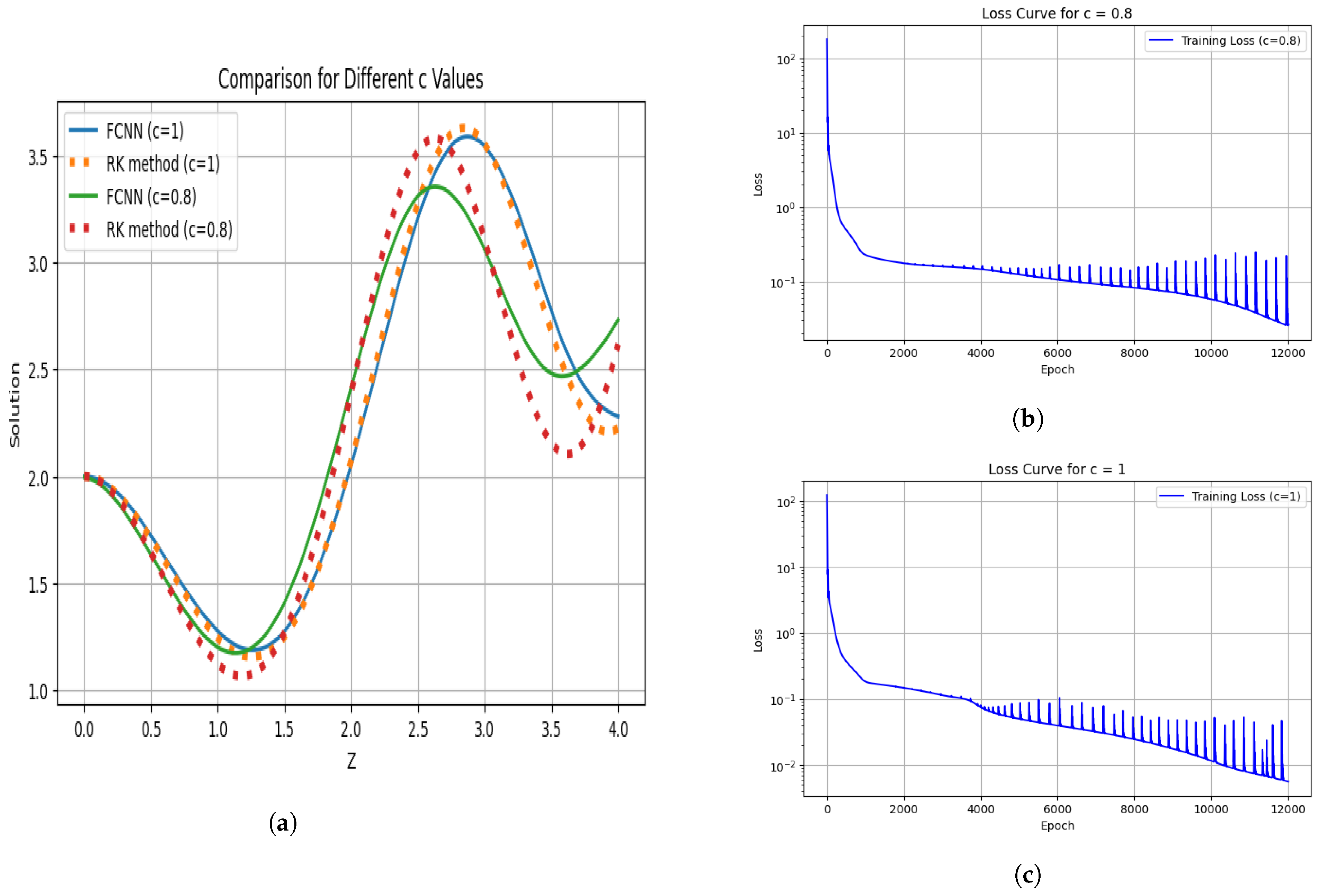
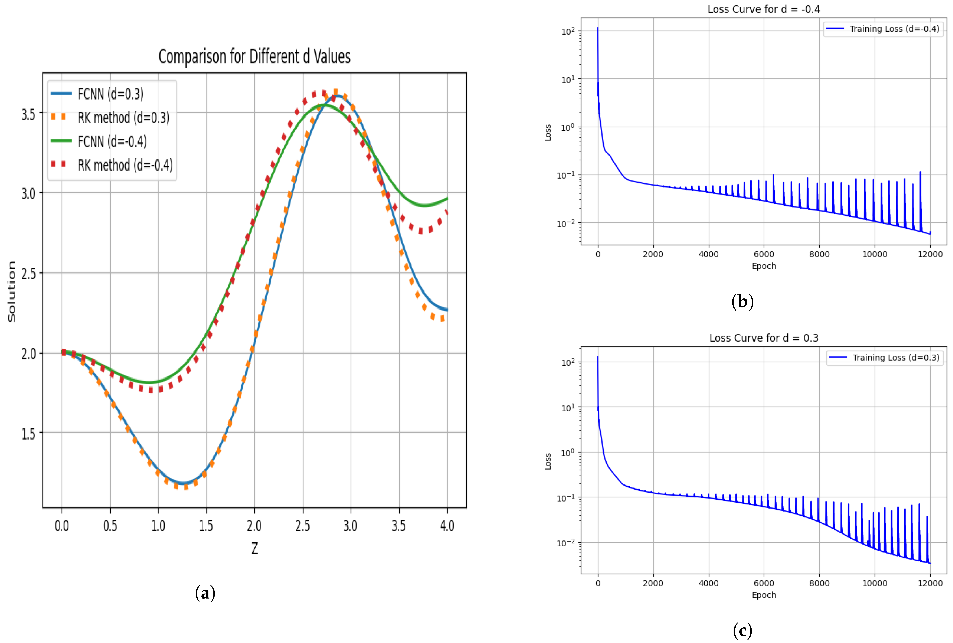
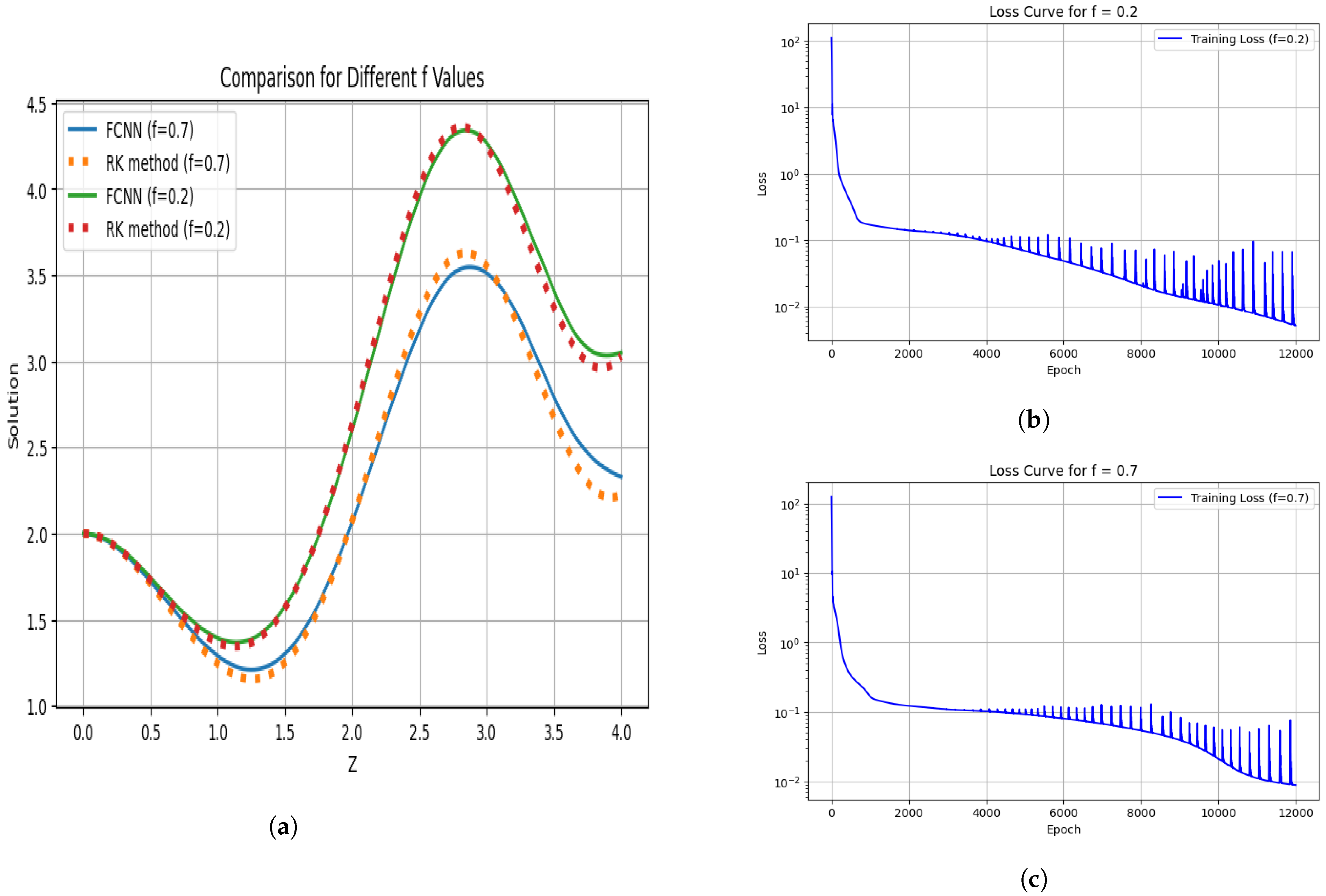
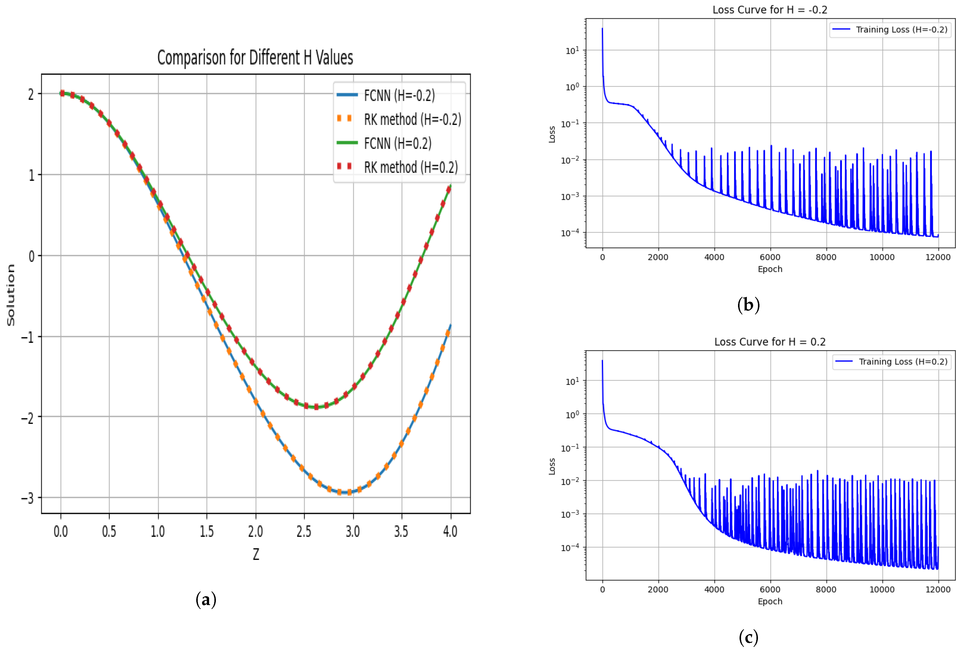
5.3. Analysis of (17) via Numerical Methods

The ODEs or PDEs are solved using an ANN-based method implemented by using computing utilities. By simplifying problem solving, making the problem domain only defined by the DE with initial or boundary conditions, the problem is defined in terms of this. This allows flexibility in testing different ANN architectures and training parameters to arrive at the best solution. Also, importantly, it is portable, as multiple types of neural network can be used, and it should be architecture-agnostic. In this framework, an FCNN is used to approximate the dependent variables. An FCNN is a basic form of DNN in which all neurons of a layer are fully connected to all neurons in the following layer. This precisely originating structure allows information to pass through the entirety of the network without any overlooked connections, and neuron groups in different layers can cooperate without the limitation of information posts. In order to predict plasma-wave dynamics, the FCNN was used for optimization in this study. Three layers of 64 neurons each were used in the network, and the hyperbolic tangent (Tanh) activation function was designed to capture nonlinear behavior. This activation function was used to satisfy the assertion of the universal approximation theorem. Based upon the theorem, a feedforward neural network with at least one hidden layer containing a finite number of neurons and a nonlinear activation function was used [45]. The Adam optimizer with a learning rate of 0.001 was used to perform the training process to facilitate stable and efficient convergence. It was trained over 12,000 epochs in order for the network to learn the underlying patterns and dynamics of the plasma system. The Adam optimizer was selected due to the support of the adaptive learning rate and the improvement in the model’s ability to handle the highly nonlinear and complex plasma dynamics.

A detailed analysis of the DNN method was performed and compared to a new numerical technique using the fourth-order Runge–Kutta (RK) method. The standard reported error norm is the $L^2$ norm via the nn.MSELoss() function. Both the DNN-based approach and the RK method were carefully used to solve Equation (17) with IVP $u^{\prime }\left(0\right)=2$ and $u\left(0\right)=0$. The loss in our model had two main terms: the residual loss, defined by the initial system of governing differential equations; and the loss ensuring the initial conditions. The difference between the actual and the predicted functions was reduced to a minimum by making sure that the predicted functions approximated towards the actual functions that held the answers. Variables undergo a first-order re-formulation of the initial second-order ODE, with the derivation performed through automatic differentiation. Moreover, the initial conditions were also imposed strictly using a weighted mean squared error term. This is a structure that makes sure that the circuit learns solutions that are consistent with the initial constraints and with the physical consistency of the solution.

In the reduced form of the equation, a constant equation is assumed for this purpose. We performed a comparative evaluation between the DNN-based method and the RK technique, on the basis of which we concluded that the DNN-based method is much more accurate and efficient than the RK method in generating consistent and plausible results for parameterized problems. The approximation was performed using two neural networks of a first-order ODE system in terms of $u\left(t\right)$ and $v\left(t\right)$ (say ${\mathcal{N}}_u$ is the trial solution for $u\left(t\right)$ and ${\mathcal{N}}_v$ is for $v\left(t\right)$), and the initial conditions were enforced as a penalty term in the loss. ${\mathcal{R}}_1$ and ${\mathcal{R}}_2$ are the residuals of the first and second equations of the system of ODEs. The total loss is

$${\mathcal{L}}_{\mathrm{total}}=\parallel {\mathcal{R}}_1{\left(t\right)\parallel }^2+{\parallel {\mathcal{R}}_2\left(t\right)\parallel }^2+10\left({∥{\mathcal{N}}_u(0;{\theta }_u)-2∥}^2+{∥{\mathcal{N}}_v(0;{\theta }_v)∥}^2\right).$$

The main objective is to minimize this loss through the Adam optimizer learning the parameters of the network ${\theta }_u$ and ${\theta }_v$ with one input and one output layer, along with two hidden layers of size 64, using $tanh$ as the activation function.

The discrepancies between the two methods were thoroughly investigated, and the factors that underlie the discrepancies are discussed. This general agreement verifies the reliability of the proposed DNN-based solution of the wave function equation. The results are relevant for plasma physics because the correct representation of wave functions and their solution in the wave problem are essential to understand wave propagation and wave interaction phenomena.

The training is shown in Figure 3 below for each time up to 12,000 epochs. By changing the weights of the network during the training process, the loss can be reduced; optimization methods are useful in this context. A comparison between the DNN-based approach and the numerical method is shown. Moreover, it can be observed that the runtimes for the FCNN and RK methods are 78.30 s and $0.0081$ s, respectively. Additionally, the RK method was stable and precise, and the FCNN needed a long training time, and it was tuning-sensitive. Being parameterized, the FCNN scales better to parameterized problems. The error heatmap for the FCNN is presented in Figure 4a and the phase portraits for both methods are presented in Figure 4b.

A heatmap of the error was used to evaluate the predictive capability of the FCNN compared to that of the RK method. In the beginning, very low error was observed, which shows a high degree of agreement between the two methods. But, with as increase in time, error propagation was realized and there was variation as well as huge deviation in the later time steps. As it turned out, although the FCNN was quite useful at picking up the local dynamics, it had a limited long-term predictive accuracy because of the cumulative error accumulation. In the phase diagram, a qualitative comparison between the RK method and the FCNN for the dynamical system is shown. The matching of the behavior in the first spiral proves that the neural network has accurate behavior in the short term. But as the time progresses, divergence becomes more pronounced and there are phase and amplitude errors in the outer loops. In plasma physics, the behavior of waves, instabilities, and nonlinear structures is governed by coefficients. So, it is important to study the individual behavior of the coefficients. In plasma physics, coefficients are used to stabilize Langmuir waves or the collapse of waves in high-intensity laser plasma systems through the nonlinearity induced in the quadratic coefficient. In Figure 5, it is observed that the wave profile broadens when the parameter $\mathsf{a}=1$. In contrast, an increase in the wave amplitude is observed when the parameter $\mathsf{a}=-0.9$. It is also shown that a change in the value of the quadratic nonlinear coefficient has a small influence on the training of the FCNN, whose predicted curves of wave functions are very close to the wave function curves generated by the RK method. The results imply that quadratic nonlinearity is important for the stability and dynamical behavior of Langmuir waves in this system.

It was determined that the coefficient of cubic nonlinearities is a primary determining factor in the prevention of wave collapse and the formation of unstable plasma behavior. It was proven that a nonlinear cubic increase leads to stabilization of the wave amplitude. Figure 6 shows the behavior for the parameter $\mathsf{b}$, as indicated. It is shown that for positive values of $\mathsf{b}$ the amplitude is smaller, but for negative values of $\mathsf{b}$, it increases. In addition, for the given specified epoch value, the training performance of the specified epoch value is supported by a unit increase in another value of b. These results reveal the importance of parameter tuning to suppress the most important cubic nonlinearities that contribute to wave dynamics and instability.

Moreover, the effects of changes in the dispersion coefficient are analyzed in Figure 7. In magnetized plasmas, dispersion is important and has been observed to support the formation of KdV solitons, but the physical origin of this is not understood. In the context of ion acoustic waves, it has been found that enhanced dispersion increases wave coherence and attenuates turbulence. The graphical analysis shows that small variations in dispersion coefficients cause significant gaps between the solutions obtained by the FCNN method and the RK method. This implies that even very small differences in dispersion can cause significant variations in plasma system numerical solutions, i.e., the FCNN and RK methods.

In addition, wave propagation with respect to dispersion was investigated. Positive dissipation enhances the steepening of the nonlinear wave and therefore calculates a higher amplitude and soliton-like structures, as shown in Figure 8. In contrast, negative dissipation results in the spreading of the wave and reduced steepening, giving broader profiles with reduced peak amplitude. These results lead to insights into the wave dynamics in ion acoustic and magnetized plasma environments.

The stability of plasma depends on the damping or growth of plasma waves, in which the energy of the waves is dissipated with time. Named collisional damping and Landau damping, damping is due to particle interaction and increases resistance to wave motion; damping transfers wave energy to particles, reducing the amplitude. Higher values of the damping function lead to faster energy dissipation and decreased wave strength. The wave function variation for damping values of 0.2 and 0.7 is shown in Figure 9; there is very little computational error in the numerical method.

The dynamical behavior of the wave function for different values of $\mathsf{H}$ is shown in Figure 10. In this way, the energy input and wave excitation dynamics can be controlled by an external forcing term $\mathsf{H}$. For $\mathsf{H}>0$, the stable, lower-energy modes that would not grow much are excited. The system is destabilized by $\mathsf{H}<0$ and higher energy, and unstable modes are found to grow. Despite the values differing by one unit for $\mathsf{H}=0.2$ and $\mathsf{H}=-0.2$, we observe that changes in $\mathsf{H}$ have a negligible effect on the wave function. From the analysis, the FCNN training results are well aligned with the curve we can obtain with the RK method, showing that the model is not very sensitive to variations in $\mathsf{H}$.

In Figure 11, the impact of $\lambda$ is shown. A higher $\lambda$ reduces the amplitude due to stronger dispersion, nonlinear saturation, and energy loss. A lower $\lambda$ increases the amplitude due to weaker dispersion and better energy retention. The reverse behavior in this case is that of competition between nonlinearity and dispersion in plasma waves, and the alignment between the FCNN training results and the curve obtained using the RK method allows us to conclude that the model is robust to variations in $\lambda$, too.

6. Conclusions

Symmetry-based methods have been used to treat the Gardner equation, and a general Lie symmetry classification has been developed with various forms of functional dependence of its coefficients. The reduced forms have been solved using the power-series method, as a result of which traveling-wave solutions are obtained in the case of constant coefficients, and also more generally without the cubic nonlinearity. To illustrate the involvement of nonlinear terms in the dynamics of waves, several graphical analyses have been presented, showing clear and contrasting behavior between both of these situations. The simplified expression that is acquired by the traveling-wave transformation has been further investigated with the help of fully connected artificial neural networks in terms of its compatibility within the field of plasma physics and comparisons have been drawn thereafter with the classical RK technique. The accuracy has been observed to significantly deviate in some of the parametric variations, especially with regard to small variations in the dispersion parameters, and the factors of dissipative, perturbative, and external forces have been determined to be insignificant. The trend exhibited by the loss curve as the training progressed established the sensitivity of the wave variables, but the fluctuation was minimal in the same training circumstances. These observations have been supported via further analyses using error heatmaps and phase diagrams. The results are the confirmation of the plausibility of the use of machine learning tools in complex nonlinear wave science and the demonstration of their potential in determining the dynamics of plasma.

7. Future Directions

Further research will also involve a detailed classification of the Lie symmetries of the stated equation to provide improved theoretical insights on their applicability in real-life situations. Also, since automatic differentiation has been found to solve analytical conditions in solving multiple cases of differential equations, the analysis will then be systematically extended to include both constant and variable coefficients, through addressing sensitivities on the FCNN platform. It will thus be easier to understand complex phenomena at a deeper level and extend the applicability of the equation to areas of nonlinear dynamics and mathematical physics. The existence, uniqueness, and stability of the numerical problem will be provided and evaluated comprehensively regarding the issue of numerical stability, the error growth, and proper posing of the Gardner equation with variable coefficients. Error bounds of discretization will be found for the proposed novel method and stability will be proven using such methods as von Neumann analysis or Lyapunov-based exploitation, especially within the theories of a standard behavior in ordinary differential equations, such as integrability and singularities.

References

1. Tajima, T. Computational Plasma Physics: With Applications to Fusion and Astrophysics; CRC Press: Boca Raton, FL, USA, 2018. [Google Scholar]
2. Zhou, T.Y.; Tian, B.; Shen, Y.; Gao, X.T. Auto-Bäcklund transformations and soliton solutions on the nonzero background for a (3 + 1)-dimensional Korteweg-de Vries-Calogero-Bogoyavlenskii-Schif equation in a fluid. Nonlinear Dyn. 2023, 111, 8647–8658. [Google Scholar] [CrossRef]
3. Cheng, C.D.; Tian, B.; Hu, C.C.; Shen, Y. Line-rogue waves, transformed nonlinear waves and their interactions for a (3 + 1)-dimensional Korteweg-de Vries equation in a fluid. Phys. Lett. A 2023, 480, 128970. [Google Scholar] [CrossRef]
4. Liu, J.G.; Zhu, W.H.; Zhou, L.; Xiong, Y.K. Multi-waves, breather wave and lump–stripe interaction solutions in a (2 + 1)-dimensional variable-coefficient Korteweg–de Vries equation. Nonlinear Dyn. 2019, 97, 2127–2134. [Google Scholar] [CrossRef]
5. Hao, X.; Lou, S.Y. Higher-dimensional integrable deformations of the modified KdV equation. Commun. Theor. Phys. 2023, 75, 075002. [Google Scholar] [CrossRef]
6. Gao, X.Y. Two-layer-liquid and lattice considerations through a (3 + 1)-dimensional generalized Yu-Toda-Sasa-Fukuyama system. Appl. Math. Lett. 2024, 152, 109018. [Google Scholar] [CrossRef]
7. Wazwaz, A.M.; Xu, G.Q. An extended modified KdV equation and its Painlevé integrability. Nonlinear Dyn. 2016, 86, 1455–1460. [Google Scholar] [CrossRef]
8. El-Monier, S.Y.; Atteya, A. Dust-acoustic Gardner solitons in cryogenic plasma with the effect of polarization in the presence of a quantizing magnetic field. Z. Naturforschung A 2021, 76, 121–130. [Google Scholar] [CrossRef]
9. Jhangeer, A.; Hussain, A.; Junaid-U-Rehman, M.; Baleanu, D.; Riaz, M.B. Quasi-periodic, chaotic and travelling wave structures of modified Gardner equation. Chaos Solitons Fractals 2021, 143, 110578. [Google Scholar] [CrossRef]
10. Helfrich, K.R.; Ostrovsky, L. Effects of rotation and topography on internal solitary waves governed by the rotating Gardner equation. Nonlinear Process. Geophys. 2022, 29, 207–218. [Google Scholar] [CrossRef]
11. Liu, H.D.; Tian, B.; Feng, S.P.; Chen, Y.Q.; Zhou, T.Y. Integrability, bilinearization, Bäcklund transformations and solutions for a generalized variable-coefficient Gardner equation with an external-force term in a fluid or plasma. Nonlinear Dyn. 2024, 112, 12345–12359. [Google Scholar] [CrossRef]
12. Liu, Y.; Gao, Y.T.; Sun, Z.Y.; Yu, X. Multi-soliton solutions of the forced variable-coefficient extended Korteweg–de Vries equation arisen in fluid dynamics of internal solitary waves. Nonlinear Dyn. 2011, 66, 575–587. [Google Scholar] [CrossRef]
13. Liu, Y.P.; Gao, Y.T.; Wei, G.M. Integrable aspects and soliton interaction for a generalized inhomogeneous Gardner model with external force in plasmas and fluids. Phys. Rev. E—Stat. Nonlinear Soft Matter Phys. 2013, 88, 053204. [Google Scholar] [CrossRef]
14. Liu, H.D.; Tian, B.; Chen, Y.Q.; Cheng, C.D.; Gao, X.T. N-soliton, H th-order breather, hybrid and multi-pole solutions for a generalized variable-coefficient Gardner equation with an external force in a plasma or fluid. Nonlinear Dyn. 2025, 113, 3655–3672. [Google Scholar] [CrossRef]
15. Meng, Q.; He, B.; Liu, W. Exact similarity and traveling wave solutions to an integrable evolution equation for surface waves in deep water. Nonlinear Dyn. 2018, 92, 827–842. [Google Scholar] [CrossRef]
16. Liu, H.; Bai, C.L.; Xin, X.; Zhang, L. A novel Lie group classification method for generalized cylindrical KdV type of equation: Exact solutions and conservation laws. J. Math. Fluid Mech. 2019, 21, 55. [Google Scholar] [CrossRef]
17. Olver, P.J. Applications of Lie Groups to Differential Equations; Springer Science & Business Media: Berlin/Heidelberg, Germany, 1993; Volume 107. [Google Scholar]
18. Bluman, G.W. Applications of Symmetry Methods to Partial Differential Equations; Springer: Berlin/Heidelberg, Germany, 2010. [Google Scholar]
19. Ovsiannikov, L.V.E. Group Analysis of Differential Equations; Academic Press: Cambridge, MA, USA, 2014. [Google Scholar]
20. Bluman, G.W.; Kumei, S. Symmetries and Differential Equations; Springer Science & Business Media: Berlin/Heidelberg, Germany, 2013; Volume 81. [Google Scholar]
21. Ibragimov, N.H. Selected Works; ALGA Publications BTH: Karlskrona, Sweden, 2006; Volume II. [Google Scholar]
22. Popovych, R.O.; Vaneeva, O.O. More common errors in finding exact solutions of nonlinear differential equations: Part I. Commun. Nonlinear Sci. Numer. Simul. 2010, 15, 3887–3899. [Google Scholar] [CrossRef]
23. de la Rosa, R.; Gandarias, M.L.; Bruzón, M.S. On symmetries and conservation laws of a Gardner equation involving arbitrary functions. Appl. Math. Comput. 2016, 290, 125–134. [Google Scholar]
24. Vaneeva, O.; Kuriksha, O.; Sophocleous, C. Enhanced group classification of Gardner equations with time-dependent coefficients. Commun. Nonlinear Sci. Numer. Simul. 2015, 22, 1243–1251. [Google Scholar] [CrossRef]
25. Abohamer, M.K.; Awrejcewicz, J.; Amer, T.S. Modeling of the vibration and stability of a dynamical system coupled with an energy harvesting device. Alex. Eng. J. 2023, 63, 377–397. [Google Scholar] [CrossRef]
26. Zhao, Y.; Jiang, C.; Vega, M.A.; Todd, M.D.; Hu, Z. Surrogate modeling of nonlinear dynamic systems: A comparative study. J. Comput. Inf. Sci. Eng. 2023, 23, 011001. [Google Scholar] [CrossRef]
27. Bukhari, A.H.; Sulaiman, M.; Raja, M.A.Z.; Islam, S.; Shoaib, M.; Kumam, P. Design of a hybrid NAR-RBFs neural network for nonlinear dusty plasma system. Alex. Eng. J. 2020, 59, 3325–3345. [Google Scholar] [CrossRef]
28. Ul Rahman, J.; Makhdoom, F.; Ali, A.; Danish, S. Mathematical modeling and simulation of biophysics systems using neural network. Int. J. Mod. Phys. B 2024, 38, 2450066. [Google Scholar] [CrossRef]
29. Ul Rahman, J.; Danish, S.; Lu, D. Deep neural network-based simulation of Sel’kov model in glycolysis: A comprehensive analysis. Mathematics 2023, 11, 3216. [Google Scholar] [CrossRef]
30. Onder, I.; Secer, A.; Ozisik, M.; Bayram, M. On the optical soliton solutions of Kundu–Mukherjee–Naskar equation via two different analytical methods. Optik 2022, 257, 168761. [Google Scholar] [CrossRef]
31. Goswami, A.; Singh, J.; Kumar, D.; Gupta, S. An efficient analytical technique for fractional partial differential equations occurring in ion acoustic waves in plasma. J. Ocean. Eng. Sci. 2019, 4, 85–99. [Google Scholar] [CrossRef]
32. Iqbal, N.; Chughtai, M.T.; Ullah, R. Fractional study of the non-linear Burgers’ equations via a semi-analytical technique. Fractal Fract. 2023, 7, 103. [Google Scholar] [CrossRef]
33. Mustafa, I.; Hashemi, M.S.; Aliyu, A. Exact solutions and conservation laws of the bogoyavlenskii equation. Acta Phys. Pol. A 2018, 133, 1133–1137. [Google Scholar] [CrossRef]
34. Inc, M.; Yusuf, A.; Aliyu, A.I.; Baleanu, D. Lie symmetry analysis and explicit solutions for the time fractional generalized Burgers–Huxley equation. Opt. Quantum Electron. 2018, 50, 94. [Google Scholar] [CrossRef]
35. Huang, Y.; Sun, S.; Duan, X.; Chen, Z. A study on deep neural networks framework. In Proceedings of the 2016 IEEE Advanced Information Management, Communicates, Electronic and Automation Control Conference (IMCEC), Xi’an, China, 3–5 October 2016; pp. 1519–1522. [Google Scholar]
36. Madhiarasan, M.; Louzazni, M. Analysis of artificial neural network: Architecture, types, and forecasting applications. J. Electr. Comput. Eng. 2022, 2022, 5416722. [Google Scholar] [CrossRef]
37. Tuan, N.M.; Kooprasert, S.; Sirisubtawee, S.; Meesad, P. The bilinear neural network method for solving Benney-Luke equation. Partial. Differ. Equ. Appl. Math. 2024, 10, 100682. [Google Scholar] [CrossRef]
38. Zhang, R.F.; Li, M.C. Bilinear residual network method for solving the exactly explicit solutions of nonlinear evolution equations. Nonlinear Dyn. 2022, 108, 521–531. [Google Scholar] [CrossRef]
39. Xie, X.R.; Zhang, R.F. Neural network-based symbolic calculation approach for solving the Korteweg–de Vries equation. Chaos Solitons Fractals 2025, 194, 116232. [Google Scholar] [CrossRef]
40. Raissi, M.; Perdikaris, P.; Karniadakis, G.E. Physics-informed neural networks: A deep learning framework for solving forward and inverse problems involving nonlinear partial differential equations. J. Comput. Phys. 2019, 378, 686–707. [Google Scholar] [CrossRef]
41. Kumar, R.; Kumar, A.; Kumar, A. Dynamic Behavior of Coupled mKdV–Calogero–Bogoyavlenskii–Schiff Equations in Fluid Dynamics. Differ. Equ. Dyn. Syst. 2025, 1–20. [Google Scholar] [CrossRef]
42. Tanwar, D.V.; Kumar, R. Kinks and soliton solutions to the coupled Burgers equation by Lie symmetry approach. Phys. Scr. 2024, 99, 075223. [Google Scholar] [CrossRef]
43. Kumar, R.; Pandey, K.S.; Yadav, S.K.; Kumar, A. Some more variety of analytical solutions to (2+1)-Bogoyavlensky-Konopelchenko equation. Phys. Scr. 2024, 99, 045240. [Google Scholar] [CrossRef]
44. Raza, A.; Mahomed, F.M.; Zaman, F.D.; Kara, A.H. Optimal system and classification of invariant solutions of nonlinear class of wave equations and their conservation laws. J. Math. Anal. Appl. 2022, 505, 125615. [Google Scholar] [CrossRef]
45. Winkler, D.A.; Le, T.C. Performance of deep and shallow neural networks, the universal approximation theorem, activity cliffs, and QSAR. Mol. Inform. 2017, 36, 1600118. [Google Scholar] [CrossRef]
Figure 1. Graphical representation of wave function presented in (24), with f = 6 ; C = 4 , a = 2 , b = 3 , c = 0.1 , C 0 = 2 , d = 2 , H = 1 , and λ = 3 . (a) 3D dynamical behavior. (b) 2D graph of wave function at different times.
Symmetry 17 01218 g001
Figure 2. Graphical representation of the wave function for different times with C 1 = 4 , a = 2 , H = 3 , and C 0 = 2 . (a) 3D dynamical behavior. (b) 2D graph of wave function at different times.
Symmetry 17 01218 g002
Figure 3. The comparison graph along with the loss curve during training with H = 4 , a = 1 , b = 0.2 , d = 0.3 , λ = 0.1 , f = 0.7 , and c = 1 . (a) Comparison between FCNN and RK techniques. (b) Loss curve during training.
Symmetry 17 01218 g003
Figure 4. Error analysis and phase diagram of FCNN and RK for H = 4 , a = 1 , b = 0.2 , d = 0.3 , λ = 0.1 , f = 0.7 , and c = 1 . (a) Absolute error analysis between FCNN and RK methods over time. (b) Phase diagram comparison of FCNN and RK.
Symmetry 17 01218 g004
Figure 5. Wave function for a = 0.9 and a = 1 with loss curve during training when H = 4 , b = 0.2 , d = 0.3 , λ = 0.1 , f = 0.7 , and c = 1 . (a) Comparison graph for different values of a . (b) Loss curve during training with a = 0.4 . (c) Loss curve during training with a = 1 .
Symmetry 17 01218 g005
Figure 6. Wave function for b = 0.2 and b = 0.2 with loss curve during training when H = 4 , a = 1 , d = 0.3 , λ = 0.1 , f = 0.7 , and c = 1 . (a) Comparison graph for different values of b . (b) Loss curve during training with b = 0.2 . (c) Loss curve during training with b = 0.2 .
Symmetry 17 01218 g006
Figure 7. Wave function for c = 0.8 and c = 1 with loss curve during training when H = 4 , a = 1 , d = 0.3 , λ = 0.1 , f = 0.7 , and b = 0.2 . (a) Comparison graph for different values of c . (b) Loss curve during training with c = 0.8 . (c) Loss curve during training with d = 1 .
Symmetry 17 01218 g007
Figure 8. Wave function for d = 0.4 and d = 0.3 with loss curve during training when H = 4 , a = 1 , d = 0.3 , l = 0.1 , f = 0.7 , and b = 0.2 . (a) Comparison graph for different values of d . (b) Loss curve during training with d = 0.4 . (c) Loss curve during training with d = 0.3 .
Symmetry 17 01218 g008
Figure 9. Wave function for f = 0.2 and f = 0.7 with loss curve during training when H = 4 , a = 1 , d = 0.3 , λ = 0.1 , b = 0.2 , and c = 1 . (a) Comparison graph for different values of f . (b) Loss curve during training with f = 0.2 . (c) Loss curve during training with f = 0.7 .
Symmetry 17 01218 g009
Figure 10. Wave function for H = 0.2 and H = 0.2 with loss curve during training when c = 1 , a = 1 , d = 0.3 , 0.1 , f = 0.7 , and b = 0.2 . (a) Comparison graph for different values of H . (b) Loss curve during training with H = 0.2 . (c) Loss curve during training with H = 0.2 .
Symmetry 17 01218 g010
Figure 11. Wave function for λ = 0.4 and λ = 0.1 with loss curve during training when H = 4 , a = 1 , d = 0.3 , d = 0.3 , f = 0.7 , and b = 0.2 . (a) Comparison graph for different values of λ . (b) Loss curve during training with λ = 0.4 . (c) Loss curve during training with λ = 0.1 .
Symmetry 17 01218 g011