Abstract
Precisely deciding potential suppliers enables companies to engage with high-caliber partners that fulfill their strategic development requirements, bolster their core competitiveness, and foster sustainable market growth. To mitigate the challenges enterprises face in selecting appropriate suppliers, a recommendation method for potential suppliers tailored to a small-sized dataset is proposed. This approach employs an enhanced Graph Convolutional Neural Network (GCNN) to resolve the accuracy deficiencies in supplier recommendations within a limited dataset. Initially, a supply preference network is created to ascertain the topological relationship between the company and its suppliers. Subsequently, the GCNN is enhanced through dual-path refinements in network structure and loss function, culminating in the adaptive feature perception model. Thereafter, the adaptive feature perception model is employed to adaptively learn the topological relationship and extract the company’s procurement preference vector from the trained model. A matching approach is employed to produce a recommended supplier list for the company. A case study involving 143 publicly listed companies is presented, revealing that the proposed method markedly enhances the accuracy of potential supplier recommendations on a small-sized dataset, thereby offering a dependable and efficient approach for enterprises to effectively evaluate potential suppliers with limited data.
1. Introduction
In the current business environment, the supply chain is becoming more complex and competitive, and the significance of recommending potential suppliers cannot be overstated. A recommended potential supplier, identified through trustworthy means, is essential for a business’s success [1,2,3]. To enhance supply chain stability, firms can mitigate the risk of disruptions in raw material or service provision by incorporating dependable potential suppliers, hence ensuring seamless operations [4,5]. Regarding cost-effectiveness, recommended suppliers may provide more advantageous pricing, superior quality items, or more efficient delivery schedules, all of which can contribute to lowering the enterprise’s overall expenses. Furthermore, recommended suppliers serve as catalysts for supply chain innovation, since they frequently introduce novel ideas and technologies that enable enterprises to sustain a competitive advantage in the market. Consequently, precisely identifying prospective suppliers is essential for the operational efficiency of businesses and holds substantial importance for augmenting their competitiveness [6,7,8].
While significant, the task of recommending potential suppliers presents substantial challenges, particularly regarding methodology. Numerous approaches have been explored in academia and industry. Many academics have conducted useful research on approaches for recommending suppliers. Bowen et al. [5] computed varied node centralities for the focus corporations and other entities within their supply networks to enhance supply chain visibility to prominent global companies. Lee et al. [9] introduced business partner recommendation methods, termed deep business partner recommendation models, designed to autonomously offer potential business partners. Tu et al. [10] developed an extensive knowledge graph to depict the actual automotive supply chain network in China. A Graph Neural Network (GNN)-based system is proposed that leverages interaction data between customers and suppliers to offer alternative suppliers from the knowledge graph. Chen et al. [11] developed a two-party game model and a cusp catastrophe model from the perspective of the mask green supply chain and analyzed the strategic choices of retailers and suppliers in the supply chain affected by the risk of capital limitations and overstock. Beyond these graph-centric approaches, recent studies address the challenge of sparse data through techniques like meta-learning (e.g., MAML for few-shot learning (Wang et al.) [12]), transfer learning (e.g., pre-training on auxiliary domains or knowledge distillation (Liu et al.) [13]), and hybrid models combining matrix factorization with attention mechanisms. Synthetic data generation, such as via GAN (Chatterjee et al.) [14], has also been explored to mitigate sparsity. However, while effective for data sparsity, these non-graph methods often face limitations in capturing the complex topological dependencies and relational structures that are inherent and crucial within supply chains, which graph methods explicitly model. Although these methods advance the field, they share a critical dependency: they typically require large volumes of data to achieve high recommendation accuracy. This data dependency becomes a significant bottleneck in scenarios characterized by small-sized datasets, which are common in practice. Recommending possible suppliers in a small-sized dataset constitutes a sparse recommendation challenge, where data sparsity hampers models’ ability to accurately discern customer preferences and supplier attributes [15,16,17]. Therefore, effectively recommending potential suppliers under small-data constraints remains a critical and under-addressed research problem.
To tackle the challenge of sparse data in supplier recommendation, graph-based learning techniques, particularly Graph Convolutional Neural Network (GCNN), offer promising potential. GCNN is a deep learning architecture that adapts convolution operations from conventional image or grid data to graph data. Its fundamental purpose is to produce node representations by consolidating feature information from the nodes and their adjacent counterparts [18,19,20]. Presently, it is extensively utilized in domains such as social network analysis, knowledge graphs, and recommendation systems [21,22,23,24]. Liu et al. [25] introduced an innovative sentiment classification model that integrates a Chinese syntactically dependent tree with graph convolution. The proposed approach offers an innovative research methodology for the identification of public opinion within social networks. Mao et al. [26] presented a knowledge aggregation fault diagnosis model that enhances the graph convolutional network and integrates it into the knowledge graph-based fault detection framework. Liu et al. [27] developed a cohesive network to encapsulate multi-behavior information, demonstrating the application of a multi-behavior Graph Convolutional Neural Network for multi-behavior recommendations. He et al. [28] introduced an enhanced collaborative filtering methodology for recommendation systems based on graph convolutional networks. The model utilized the vector representations of the aggregated attribute graph as input [29,30,31,32]. In contrast to GNN, GCNN retains the processing capabilities of GNN for graph-structured data. The benefit resides in the rigorous definition of convolution operations grounded in graph signal processing or spatial aggregation, which can more systematically leverage the local structure information of the graph [33,34,35,36]. This capability makes GCNN a strong candidate for modeling complex relationships in supplier recommendation systems. However, their effectiveness in the specific context of sparse, small-scale supplier datasets with unique structural characteristics and feature availability constraints remains an open challenge.
Although supplier recommendation systems have advanced, a research gap persists in small-scale data scenarios. Existing approaches—such as graph neural networks and matrix factorization—heavily rely on large-scale data to achieve high accuracy, resulting in sub-optimal recommendations under sparse data conditions. Traditional graph convolution methods employ symmetric normalization and generic loss functions that dilute critical preference signals within sparse supply networks. Moreover, current methods require the simultaneous input of explicit features for both enterprises and suppliers, limiting their adaptability when enterprise attributes are unavailable. Therefore, this study aims to address these gaps by (1) refining the graph convolutional network to effectively preserve critical preference signals in sparse supply networks, (2) designing a loss function that balances feature discriminability with reconstruction capability under limited data, and (3) developing a recommendation capability that relies solely on supplier features, thereby minimizing dependence on enterprise attributes. To tackle these challenges, we propose dual refinements: on the one hand, one-sided normalization preserving asymmetric procurement influences; on the other hand, a hybrid loss balancing feature discrimination/reconstruction. Motivated by the need for effective small-data supplier recommendations and the strengths of GCNNs in handling relational data with limited information, this paper proposes a novel approach centered on an adaptive feature perception model, which refines the GCNN architecture.
The primary technical framework of this paper is illustrated in Figure 1. A potential supplier recommendation approach using an adaptive feature perception model for a small-sized dataset is proposed. Initially, a supply preference network is established to derive the topological relationship graph between the enterprise and the supplier. Subsequently, the GCNN is enhanced through dual-path refinements in model structure and hybrid loss function, culminating in the adaptive feature perception model. Among them, the constructed hybrid loss function includes a contrastive learning module and a reconstruction feature module. Then, the adaptive feature perception model is employed to adaptively learn the supply preference network and derive the purchasing preference vector of the company from the trained model. Finally, a cosine similarity-based matching strategy is used to generate a recommended supplier list for each company, and a case study involving 143 listed firms is conducted to test and evaluate the efficacy of our approach. This study primarily addresses three aspects that have not been explored in prior research. (1) An approach for recommending potential suppliers, based on an adaptive feature perception model, is proposed, demonstrating efficacy even with a sparse, small-sized dataset. This strategy can generate prospective supplier lists for enterprises. (2) The adaptive feature perception model is enhanced in two aspects: the network structure and loss function, hence improving its performance and efficacy on sparse, small-sized datasets. (3) The adaptive feature perception model requires only the supplier’s feature information during initialization, omitting the enterprise’s feature information, hence diminishing the dataset feature information requirement and enhancing the model’s adaptability to generalization.
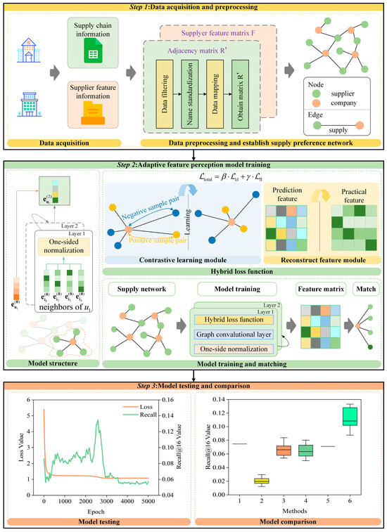
Figure 1.
The primary technical framework of this paper.
The following portions of this document are organized as outlined below. Section 2 outlines the fundamental theory of the suggested methodology. Section 3 analyses the potential supplier recommendation approach. Section 4 delineates the primary conclusions and implementation specifics of the proposed methodology, supported by empirical evidence. Ultimately, Section 5 concludes the article with a synthesis of essential points.
2. Fundamental Theory
2.1. Problem Setup
In intricate commercial procurement situations, companies have to identify possible suppliers that fulfill their requirements. Mining potential linkages between organizations and suppliers and achieving precise suggestions in small-sized datasets presents a significant challenge. This paper initially formulates a mathematical model of the problem and subsequently presents an efficient approach to address the possible supplier recommendation issue within a limited dataset. Let the company set as C = {c1, c2, …, cm} and the supplier set as S = {s1, s2, …, sn}. Construct a relationship matrix R = {rij}m×n, where element bij denotes the relationship between the i-th firm ci and the j-th supplier sj:
where the i-th firm ci purchases from the j-th supplier sj, ci is connected to sj.
Using relationship matrix R as the underlying framework, a supply preference network A is constructed by embedding supplier feature information. Then, the primary aim of this study is to identify a recommended suppliers list RL ⊆ S for each company ci, ensuring that these suppliers align with the purchasing preferences of company ci to the maximum degree. To obtain precise recommendations, a mapping function f needs to be developed, utilizing the supply preference network A and company ci, to produce a list of recommended suppliers RL. In this procedure, an adaptive feature perception model is employed to ascertain the mapping relationship. The adaptive feature perception model is represented as g(∙), where the input is the supply preference network A. By reducing the loss function L and refining the model parameters, yi represents the authentic preference vector aligned with the actual purchase behavior of the company ci.
In summary, the mathematical problem addressed is as follows: under the specified conditions of company set C, supplier set S, and supply preference network A, the objective is to optimize parameters of the adaptive feature perception model g(∙) and the matching algorithm to determine the mapping function f, thereby achieving the optimal correspondence between the recommended supplier list RL and the actual procurement preferences of the i-th company ci, specifically minimizing the loss function L(pi, yi).
2.2. Supply Preference Network
Constructing suitable data structures is essential for analyzing interactions between companies and suppliers. This study adopts a graph-structured supply preference network to model topological relationships between enterprises and suppliers. Compared with traditional data structures, graph-structured networks can comprehensively represent intricate inter-object connections while providing an efficient framework for subsequent analytical tasks and algorithmic development.
Investigate a procurement relationship network comprising a set of companies C and a set of suppliers S. Formulate a bipartite graph G = (V, E), where the vertex set V = C∪S and the edge set E delineate the commercial relationships between companies and suppliers. If the i-th company ci engages in business with the j-th supplier sj, an edge (ci, sj) exists, linking nodes ci and sj within the graph. Then, the definition of the constructed supply preference network A is as follows:
where R’ is the adjacency matrix of two rows and e columns. F is the supplier feature matrix with n rows and d columns. e and n represent the total number of edges and nodes, respectively. d represents the number of node features.
The adjacency matrix R’ is another manifestation of the relationship matrix R, which eliminates the zero items in the relationship matrix R, making its elements more concise. In the adjacency matrix R’, the initial row denotes the supplier’s node number, the next row indicates the company’s node number, and each column signifies a tangible procurement relationship. For the edge weight matrix W, it is used to describe the procurement relationship between suppliers and companies. For the supplier node feature matrix F, it is utilized to describe the qualities of the provider.
The supply preference network is pivotal in this research. It serves as an intuitive data input for the adaptive feature perception model, which adeptly captures the topological features between companies and suppliers through the convolution of the supply preference network, thereby discerning the implicit relationships among nodes. Furthermore, utilizing the supply preference network facilitates the extraction of procurement behavior patterns of companies, establishing a basis for the generation of procurement preference feature matrix. Consequently, intricate business relationships are converted into computable mathematical entities, allowing subsequent recommendation algorithms to operate efficiently on structured data, thereby augmenting the accuracy and efficacy of potential supplier recommendations.
2.3. Graph Convolutional Neural Network
GCNN is a deep learning model specifically engineered for graph-structured data. Traditional neural networks encounter difficulties with non-Euclidean graph data, whereas the GCNN model utilizes graph convolution operations to capture topological dependencies among nodes and their neighbors, thereby effectively learning intricate relationships and serving as potent instruments for graph learning tasks.
The fundamental concept of GCNN involves the iterative execution of graph convolution operations to consolidate information from adjacent nodes and progressively acquire higher-order representations for each node. Specifically, GCNN refines the features on the graph, facilitating the effective integration of neighboring nodes’ features at each convolution step, thus updating the representation of the target node. Each convolution operation consolidates the features of neighboring nodes and, in conjunction with the edge connections, revises the feature representation of the target node. This neighborhood aggregation can be formalized as follows:
where Nu and Ni denote the number of adjacent nodes for node u and node i, respectively; eul+1 and eil are the feature representations of the nodes.
The input to a typical GCNN comprises graph topology data and a node feature matrix. The graph topology data is represented by an adjacency matrix. Let the user–item interaction matrix be denoted as:
where P and Q represent the number of users and items, respectively. If user u interacts with item i, then Jᵤᵢ is 1, otherwise 0.
Subsequently, the adjacency matrix associated with the graph can be derived as follows:
Assume that each node is linked to a D-dimensional feature vector in the node feature matrix. The features may derive from node properties, one-hot encoding, and similar methods. The node feature matrix is delineated as follows:
After stacking numerous layers of graph convolution operations, the GCNN gradually widens the receptive field of the nodes and learns higher-order neighborhood information. Specifically, the propagation rule for each layer can be written as:
where E is the feature matrix of the initial state. σ(∙) represents the activation function. D is the degree matrix. (A+I) denotes the adjacency matrix with an added identity matrix to introduce self-connections, thereby preserving each node’s own information. h(l−1) denotes the hidden state vector at the (l − 1)-th layer, and W(l−1) represents the weight matrix mapping from the (l − 1)-th layer to the l-th layer.
3. Potential Supplier Recommendation Approach
3.1. Adaptive Feature Perception Model
3.1.1. Model Structure
This study pertains to a small-sized dataset, whereby the model’s feature matrix only requires supplier feature information as input. The absent feature information of the company nodes is dynamically influenced and adjusted by the supplier nodes throughout the model’s training process. The traditional GCNN model architecture, with symmetric normalization, fails to meet the aforementioned constraints. This study enhances the GCNN model architecture by proposing a “One-sided normalization” strategy.
Figure 2 illustrates the architecture of the adaptive feature perception model. A “One-sided normalization” strategy is proposed, using the reciprocal of the in-degree of destination nodes as edge weights to equilibrate the interaction between user nodes and item nodes. The model utilizes a two-layer graph convolutional network to initially aggregate local neighborhood features, subsequently propagating and merging higher-order information. Thus, efficiently extracting the multi-dimensional features and topological relationships of nodes inside the supply chain network establishes a solid feature foundation for supply chain recommendation tasks.
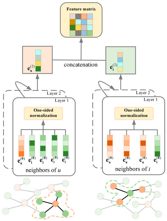
Figure 2.
Structure of the adaptive feature perception model.
The improvements to the adaptive feature perception model include the “One-sided normalization” strategy and dynamic user feature generation, specifically designed to address small-data challenges. The “One-sided normalization” prioritizes the information flow from items to users while simultaneously suppressing backpropagation from featureless user nodes—thereby protecting original item features from distortion. Crucially, user features are dynamically generated during training through layer-wise propagation. Unlike conventional GCNN, which requires pre-defined features for all nodes, this approach adaptively generates user features during the training process.
Taking the aggregation of local neighborhood features as an illustration, the model prioritizes the integration of the source node’s features into the target node’s features while reducing the influence of the source node’s topological structure on the target node. To do this, the aggregation function for adjacent node attributes in the model is delineated as follows:
where eul+1 represents the feature vector of node u at layer l+1. Nu denotes the set of neighbor nodes for node u. eil represents the feature vector of node i at layer l.
As shown in Figure 2, the gray arrows in the diagram indicate the information flow during model training. The adaptive feature perception model employs a hierarchical architecture to integrate supplier features and topological relationships. The model input is the supply preference network composed of the supplier feature matrix F and adjacency matrix R’. The first convolutional layer performs feature propagation under the “One-sided normalization” strategy, where the reciprocal of enterprise in-degrees is used as edge weights to aggregate supplier features onto enterprise nodes. This step dynamically infers missing enterprise features from supplier attributes. The second convolutional layer continues employing “one-sided normalization” to propagate higher-order neighborhood information, thereby refining the procurement preference vector. The model outputs the procurement preference vector and the optimized supplier feature matrix.
3.1.2. Hybrid Loss Function
To concurrently enhance the discriminative capacity of feature learning and the precision of feature reconstruction, we present a hybrid loss function that amalgamates two components: a contrastive learning module and a reconstruct feature module. The hybrid loss function is defined as:
where cl denotes the contrastive learning module and fl represents the reconstruct feature module. β and γ are weighting coefficients, respectively.
The hybrid loss function is derived from a weighted integration of the contrastive learning module and the reconstruct feature module, aiming to concurrently augment the discriminative capacity of the features while preserving feature consistency. The design concepts of these two fundamental components are detailed as follows: the contrastive learning module enhances the differentiation of features in the feature space by creating positive and negative sample pairs. The reconstruct feature module mitigates feature distortion by imposing similarity constraints between the input and output features. Their synergy guarantees that the model both amplifies the expressiveness of feature representations and preserves the stability of the feature space.
- Contrastive learning module
The contrastive learning component aims to improve the discriminative capacity of the user-item feature space via self-supervised learning. The main idea is to reduce the proximity of positive sample pairings while increasing the distance between negative sample pairs, hence facilitating the model’s acquisition of more distinctive feature representations. The precise execution entails the following essential steps:
Step 1: Utilizing the interaction relationships depicted by the bipartite graph G = (V, E), generate a collection of positive and negative sample pairs:
where Ppos is the set of positive sample pairs and Pneg is the set of negative sample pairs. The notation (u,i+) represents a positive sample pair, (u,i−) represents a negative sample pair, and E denotes the set of all observed interaction edges.
Step 2: The feature correlation is computed using L2-normalized cosine similarity, defined as follows:
where fu and fi are the feature vectors of user u and item i. fu·fi denotes the dot product of f with itself. ||·||2 is the L2 norm, which eliminates the effect of vector length and focuses solely on directional similarity.
Step 3: Develop a contrastive loss function grounded in the disparity of similarity between positive and negative sample pairs:
where k and k represent the set of negative sample pairs and positive sample pairs, respectively. denotes the sum of similarities for negative sample pairs, while denotes the sum of similarities for positive sample pairs.
- 2.
- Reconstruct the feature module
The primary aim of the reconstruct feature module is to ensure alignment between the model’s output features and the input features, hence avoiding distortion of the feature space due to excessive optimization of discriminability during contrastive learning. The particular execution encompasses the subsequent essential steps:
Step 1: Given that the feature matrix output by the model contains features for both users and items, and only the item features are required for feature reconstruction, the item features are extracted from the output through a segmentation operation.
Step 2: The input item features are regarded as the target features.
Step 3: Based on the target features and the output features, the reconstruction feature loss function is constructed as:
where Ni represents the total number of items, corresponds to the output feature, and fi(in) is the input feature.
The hybrid loss function plays a crucial role in mitigating data sparsity. The contrastive learning module enhances the discriminative power of the features by differentiating between positive and negative samples, which is particularly important in small-sized datasets where feature distinctions are critical. The reconstruction module ensures that the learned features remain consistent with the original input features, preventing overfitting and maintaining stability in the feature space. Together, these modules improve the robustness and accuracy of the model even when the data is limited.
3.2. Feature Matching
Feature matching serves as the core component of recommendation systems for potential suppliers, aiming to achieve accurate alignment between enterprise procurement preference vectors and supplier feature vectors, thereby identifying candidate suppliers that align with the enterprise’s strategic requirements. Under sparse and small-sized sample scenarios, the validity of feature matching directly influences the model’s generalization capability and the credibility of recommendation outcomes.
The selection of cosine similarity as the matching metric is strategically justified by two key considerations: (1) Scale invariance accommodates heterogeneous feature magnitudes (e.g., innovation scores vs. size indicators) by focusing on angular alignment while ignoring norm disparities; (2) Sparsity robustness prevents dot products’ bias toward high-norm suppliers in high-dimensional sparse spaces.
Derived from the adaptive feature perception model, feature aggregation is performed on the user–item graph, resulting in the user feature matrix and the item feature matrix , where p represents the number of users, q represents the number of items, and d denotes the feature dimension. The recommendation list is produced through the calculation of cosine similarity in the feature space, subsequently followed by Top-K selection. The recommendation potential supplier P(s) is derived directly using the subsequent formula:
where the numerator UIT computes the raw similarity matrix between users and items, while the denominator normalizes the values by multiplying the L2 norms of the user features U and the item features I, resulting in a standardized cosine similarity matrix.
Additionally, a Top-K operation is executed for each user to identify the K items exhibiting the greatest similarity. This process yields the indices of the K items exhibiting the highest similarity scores, along with their respective values, thereby generating the personalized recommendation outcomes.
3.3. Recommendation Process
This research presents a potential supplier recommendation process consisting of four stages: raw dataset, data preprocessing, modeling, and application, aimed at generating supplier recommendations specifically for a small-scale dataset. As depicted in Figure 3, each stage is rigorously organized: raw data consolidation ensures comprehensive coverage of supply chain relationships; preprocessing eliminates inconsistencies through data standardization, entity disambiguation, and feature engineering; the modeling phase adaptively learns procurement preferences via adaptive feature perception model; while the application layer translates abstract feature vectors into ranked recommendations through cosine similarity metrics. This hierarchical architecture effectively bridges the gap between raw business data and strategic decision-making, enabling enterprises to identify optimal suppliers even under data scarcity constraints.
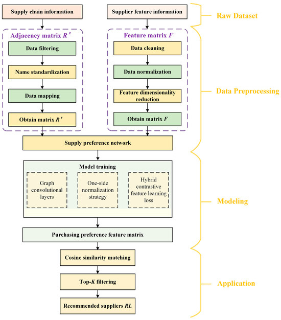
Figure 3.
Flowchart of the supplier recommendation process.
Stage 1: Raw dataset. The raw data serves as the foundation for the recommendation process, encompassing two essential components. Supply chain information meticulously documents the company and its associated supplier list, illustrating the business relationship network between the enterprise’s upstream and downstream sectors, and offering a framework for investigating new collaborative relationships. The second pertains to the supplier feature information, encompassing fundamental aspects such as technology and scale. The raw data serve as essential resources for further research and are significant sources of insights for investigating new supplier partnerships.
Stage 2: Data preprocessing. Preprocessing of the raw data is necessary to obtain the adjacency matrix and supplier feature matrix for later analysis. Data filtering is employed to eliminate invalid or erroneous entries in the adjacency matrix, while name standardization is utilized to standardize the naming format. Data mapping is executed to convert the data into an appropriate format, precisely illustrating the relationships among nodes. In constructing the supplier feature matrix, data cleaning eliminates outliers, data normalization standardizes the data range, and feature dimensionality reduction minimizes feature dimensions, eliminates redundant information, enhances data quality and analytical efficiency, thereby establishing a robust foundation for subsequent modeling.
Stage 3: Modeling. Advanced optimization utilizing typical GCNNs. A one-sided normalization strategy was presented for generating graph topologies, utilizing the reciprocal of the in-degree of destination nodes as edge weights to balance the interaction between user nodes and item nodes. The hybrid loss function, as a fitness criterion, is formulated through a weighted integration of the contrastive learning module and the reconstruction feature module, with the objective of simultaneously enhancing the discriminative power of the features and maintaining feature consistency. Utilize the structured and processed dataset to train the model, enabling it to comprehensively understand the intricate correlation features between enterprises and suppliers, subsequently extracting the enterprises’ purchasing preference feature matrix.
Stage 4: Application. A matching method utilizes the purchasing preference vector derived from the trained model to provide a recommendation list. Compute the cosine similarity between every supplier and the purchasing preference vector, then rank and identify the suppliers with the highest scores. The final outcome is a high-quality list of recommended potential suppliers, enabling companies to effectively identify partners that align with their requirements and enhance supply chain management efficiency.
4. Experiment and Analysis
4.1. Experiment Descriptions
The research data for this case study was gathered from the Chinese research data services platform (CNRDS) and the Qixinbao platform. This study is grounded in the Chinese national economic industry classification standard (GB/T 4754-2017) [37] and examines publicly listed companies in the computer, communications, and other electronic equipment manufacturing sector (industry code C39) on China’s A-share main board, along with their suppliers. Company-level data were drawn from the CNRDS database; after applying industry-classification filters and excluding companies with fewer than three suppliers, a final sample of 143 companies was retained. Supply chain relationships and supplier characteristics were obtained via the Qixinbao platform, yielding 814 suppliers, each described by four core attributes: listing status, technological innovation capability, firm type, and firm size. The computational resources utilized include an Intel Core i7-12800HX CPU, 16 GB of RAM, and an RTX 4060 laptop GPU with 8 GB. The programming environment comprises Pytorch 2.4 and Python 3.12.
To thoroughly assess the performance and effectiveness of the proposed approach, we utilized the established assessment metric of Recall. The metric is explicitly defined as follows:
where Pj(s) denotes the set of top-K predicted suppliers for the j-th listed company, while Tj(s) represents the ground-truth supplier set of the j-th listed company.
4.2. Case Study
4.2.1. Data Preprocessing
The raw data were preprocessed to ensure their validity. Missing or erroneous entries in the supplier feature information were removed. Categorical variables (firm type and firm size) were converted via one-hot encoding to render them suitable for analysis. Thus, the four core indicators were transformed into a nine-dimensional feature vector (Listed, –Innovation, State-owned enterprise, Foreign background, Private enterprise, Business background, Small-scale, Medium-scale, Large-scale), and each dimension was subsequently normalized. The result is an 814 × 9 feature matrix. Table 1 presents a subset of the information contained in this matrix.

Table 1.
Examples of suppliers’ features.
Using supply chain relationships, an adjacency matrix between publicly listed companies and suppliers was created. However, differences in entity naming prevented a direct connection between the adjacency matrix and the feature matrix. To address terminology standardization issues, we designed a unique numerical identification system that assigns each publicly listed company and supplier a unique ID and established a mapping database linking these identifiers to the corresponding entity names. Ultimately, based on this mapping technology and supply chain relationship data, a numerical-ID-centric adjacency matrix of publicly listed companies and suppliers was generated. Using supplier IDs as a foreign key, we effectively connected the adjacency matrix with the feature matrix.
Table 2 presents a selection of the matching relationships between the listed companies and their respective suppliers. At this stage, we obtained both the adjacency matrix and the feature matrix. We subsequently established a supply chain network consisting of 143 publicly traded firms and 814 suppliers, with 957 edges denoting the supply links. Python and Neo4j, a graph database with visualization features, were employed to illustrate the supply chain network, as depicted in Figure 4.
Table 2.
The supply relationship between the listed companies and their suppliers.
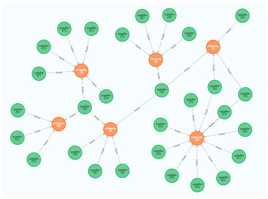
Figure 4.
Visualization of partial supply chain network in Neo4j. (Colors indicate node types: green = supplier, orange = company).
4.2.2. Experimental Evaluation
In this study, recall was selected as the primary evaluation metric to comprehensively assess the model’s capability in identifying potential suppliers. To ensure experimental reliability, the model underwent rigorous training for 5000 epochs, with an early stopping mechanism applied based on validation-set monitoring. The training process terminated at 2500 epochs when the validation loss plateaued, suggesting limited potential for further generalization gains. As shown in Figure 5, the composite training loss, consisting of weighted contrastive loss and reconstruction loss, exhibited a consistently declining trend, hence affirming effective model convergence. Notably, divergence patterns among individual loss components revealed inherent trade-offs between the dual objectives of feature discrimination and reconstruction. This observation aligns with the challenge of balancing multi-task optimization in graph-based recommendation systems, where overemphasis on one objective may compromise the other.
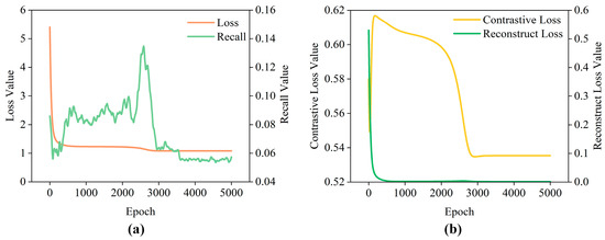
Figure 5.
The loss curves and recall performance: (a) Model training loss and Recall@16. (b) Contrastive loss and Reconstruction loss.
Analysis of Figure 5 indicates that during the first training period (0–500 epochs), the reconstruction feature loss diminished swiftly, prevailing in the overall loss optimization. This indicates that the model initially emphasized the reconstruction of input data. Simultaneously, the contrastive learning loss increased sharply, leading to a swift deterioration in recall performance. In the following phase (500–2500 epochs), the contrastive learning loss was markedly improved, signifying proficient learning of feature differentiations between positive and negative data. This optimization maximized recall and systematically balanced multi-task objectives.
To evaluate the effectiveness of the proposed method, this study compared it with five baseline methods using the evaluation metrics Recall@10 and Recall@16. Based on these two metrics, the respective 95% confidence intervals (calculated using the t-distribution) and the runtime were recorded. Since Method 1 and Method 5 are deterministic algorithms, no 95% confidence intervals are provided. The comparative results of different methods are detailed in Table 3. Among them, Method 1 directly generates the company’s procurement feature vector by calculating the average of multiple supplier feature vectors from the raw data; Method 2 employs a traditional GNN; Method 3 uses a standard GCNN model; Method 4 utilizes matrix factorization (MF); Method 5 adopts a content-based filtering (CBF) algorithm; Method 6 is the method proposed in this paper. Figure 6 presents the distribution of recommendation performance for different methods under the Recall@10 and Recall@16 metrics using box plots.
Table 3.
Comparison of the performance of different methods in Recall@10, Recall@16, and running time.
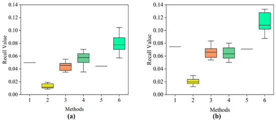
Figure 6.
Box plots of recommendation results from different methods: (a) Recall@10, (b) Recall@16.
The results in Table 3 reveal the limitations of current supplier recommendation methods when dealing with small-sized datasets. Methods that depend on learning complex patterns or interactions, such as GNN, GCNN, and MF, are significantly affected by data sparsity. Among these, GNN performs the worst. Even standard GCNN and MF show substantial performance drops compared to the proposed method, highlighting their reliance on larger datasets. Additionally, the symmetric normalization commonly used in GCNN (Method 3) seems to weaken important preference signals in the sparse supply preference network, reducing its effectiveness. Furthermore, simpler methods like Supplier Mean and CBF do not learn complex patterns but overlook valuable topological relationships between companies and suppliers, leading to suboptimal performance. They also struggle to generalize effectively to new or underrepresented entities.
The experimental results demonstrate that the proposed method exhibits significant advantages in the recall metrics. Specifically, on Recall@10, the proposed method is significantly higher than the suboptimal method, matrix factorization (MF), and all other baseline methods (such as GCNN and CBF). On Recall@16, its advantage is further amplified. Crucially, the 95% confidence intervals of the proposed method on both recall metrics show no overlap with those of the second-best performing MF, providing strong statistical evidence that its performance improvement is significant and reliable. Although our method incurs higher runtime than simpler baselines like MF or CBF, this cost remains practically acceptable for SME supplier selection—processing 143 companies in under 1 min. The recall gain over suboptimal methods justifies this marginal computational overhead for mission-critical procurement decisions.
To assess the interpretability of the recommendation results and the effectiveness of the model’s feature extraction, we selected Company 6 (C-6) and Company 142 (C-142) as representative case studies. By visualizing the recommendation lists and comparing their feature distributions, we conduct an in-depth analysis of the model’s performance in practical application scenarios. In this context, “S-n” denotes the supplier numbered n, and “C-m” denotes the listed company numbered m.
As illustrated in Figure 7, the model recommends 10 suppliers (S-49, S-45, S-44, etc.) for C-6, 3 of which (S-45, S-44, and S-43) match its actual suppliers (S-43, S-44, S-45, S-46), yielding a recall rate of 75%. However, the actual supplier, S-46, does not appear in the recommended list. For C-142, none of the 10 recommended suppliers (S-532, S-546, S-108, etc.) match its actual suppliers (S-140, S-811, S-812, S-813).

Figure 7.
Visualization of the recommended lists for Company 6 and Company 142.
To conduct a deeper investigation of the recommendation outcomes, we compare cases C-6 and C-142 by analyzing the feature distributions depicted in Figure 8. In the successful case C-6, its four actual suppliers (S-43, S-44, S-45, and S-46) demonstrate high consistency in key features. Feature 2 (Technology-Innovation) maintains a uniform value of 0.8, whereas Features 7–9 (firm size) all indicate “Large-scale.” This homogeneity enables the model’s generated procurement-preference features to achieve precise alignment with supplier characteristics, resulting in 75% recall of actual suppliers and thereby validating the model’s high precision in scenarios with well-defined requirements.
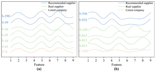
Figure 8.
The feature distribution map of listed companies and their suppliers: (a) Company 6 (C-6), (b) Company 142 (C-142).
By contrast, the four actual suppliers (S-140, S-811, S-812, and S-813) in the unsuccessful case C-142 exhibit significant heterogeneity. Feature 2 (Technology–Innovation) shows values ranging from 0.2 (S-813) to 0.8 (S-811 and S-812), with S-140 at 0.6, indicating a 0.6-point span that suggests the absence of strict technical thresholds for suppliers. Regarding Features 7–9 (firm size), the suppliers comprise large-scale (S-811, S-813), medium-scale (S-812), and small-scale (S-140) enterprises. This diversity signifies C-142’s acceptance of partners across multiple scales, while the multidimensional dispersion of features reveals its lack of consistent procurement preferences. Consequently, preference-based recommendation models prove inadequate in capturing these complex demands, ultimately generating recommendations with zero overlap with actual suppliers. This contrast demonstrates that the uniformity in a company’s supplier feature distribution constitutes a critical determinant of model performance.
Quantitative analysis of recommendation errors reveals: In case C-6, all three authentic suppliers ranked within the top 2% (S-43:2, S-44:3, S-45:16), demonstrating high precision for stable preferences; whereas a false negative sample identified through error quantification (S-46:642) exposed the model’s sensitivity to feature outliers. In case C-142, error quantification metrics confirmed all authentic suppliers significantly outperformed random expectations (average rank 299.5 vs. random baseline 407.5), with core suppliers (S-811:197, S-812:231) exhibiting tighter clustering than peripheral partners (S-813:396, S-140:374). These quantitative results demonstrate that even when not achieving Top-K recall, the model effectively elevates genuine partners above noise suppliers.
4.2.3. Ablation Study
This paper systematically analyzes the synergistic effects of loss functions and normalization strategies based on the GCNN framework. Table 4 illustrates the impact of different model components on the experimental results, where symmetric normalization and One-sided normalization are abbreviated as SN and ON, respectively. Method 1 implements a GCNN model integrating ON with the contrastive learning loss function; Method 2 implements a GCNN model combining ON with the reconstruction loss function; Method 3 applies a GCNN model using SN with the hybrid loss function; and Method 4 implements a GCNN model combining ON with the hybrid loss function, which is the combination adopted in this paper.
Table 4.
Comparative results of ablation studies based on GCNN.
As shown in Table 4, this ablation study, conducted within the GCNN framework, reveals the synergistic mechanism between the hybrid loss function and the one-sided normalization strategies. Under the fixed condition of ON, the hybrid loss function integrating contrastive learning and reconstruction learning demonstrates significantly superior feature extraction capabilities compared to single loss functions. When employing the identical hybrid loss function, ON yields statistically significant performance improvements over SN (as evidenced by non-overlapping confidence intervals), validating its effectiveness in optimizing graph structural weights. Ultimately, the combination of the hybrid loss function with ON achieves the optimal performance, providing compelling evidence that the synergistic optimization of the multi-task learning mechanism and the graph normalization strategy plays a central role in enhancing model efficacy.
4.3. Discussion
To evaluate the model’s tolerance to data deficiencies, we designed a feature masking test: randomly selecting 5–15% of supplier samples and setting all their features to zero to simulate data missingness. This procedure strictly corresponds to typical scenarios of incomplete supplier information collection in practical applications (e.g., incomplete profiles of new suppliers). The test employed 10 independent repeated trials to control for randomness, with final results presented in Table 5.
Table 5.
Performance (mean ± std) of Recall@10 and Recall@16 under different masking ratios.
Analysis of the data reveals an interesting phenomenon: While recall values under all masking conditions were lower than the baseline, the decline rate did not increase linearly. Specifically, recall values did not exhibit a monotonically decreasing trend as the masking ratio increased. For recall metrics: When the masking ratio increased from 5% to 10%, recall showed a slight decrease; however, when the masking ratio increased further to 15%, recall exhibited a small rebound. Analysis of this phenomenon suggests it may be attributed to dataset characteristics: Masking 15% of features may coincidentally remove less important or noisy features, thereby leading to a performance recovery. It is noteworthy that recall under all masking conditions remained significantly lower than the baseline, underscoring the critical importance of feature information for model performance. Nevertheless, the model’s ability to maintain a certain level of performance despite partial feature absence indicates its inherent robustness.
The hyperparameters in this experiment were meticulously tuned to optimize the model’s performance. Throughout the entire training process, all models were optimized using the Adam optimizer with a learning rate of 0.001. The weights β and γ in the hybrid loss function, which combines a contrastive learning module and a feature reconstruction module, were selected from the search space [1, 10] via grid search, as illustrated in Figure 9.
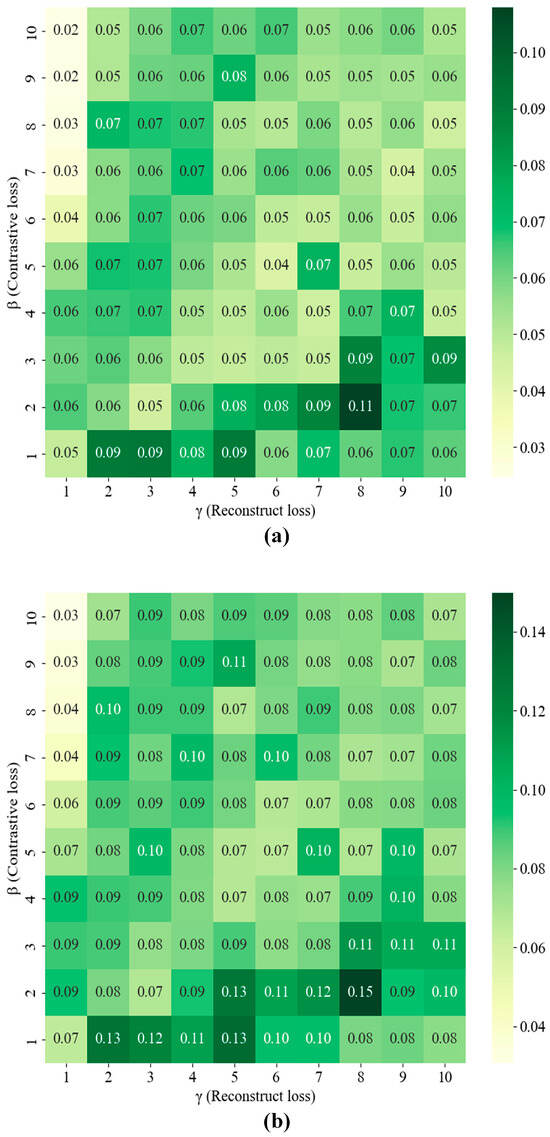
Figure 9.
Recall value under varying β (Contrastive loss) and γ (Reconstruct loss) weight coefficients: (a) Recall@10, (b) Recall@16.
While this hybrid approach enhances feature representation, it is crucial to balance these two components. If the contrastive learning module (weighted by β) dominates, the model may overfit the training data, capturing noise instead of underlying patterns. Conversely, if the reconstruct feature module (weighted by γ) dominates, the model might underfit, failing to learn complex supplier-customer relationships and potentially under-representing certain supplier types. To avoid these pitfalls and achieve an optimal trade-off, the weighting coefficients (β and γ) required careful tuning.
This careful balancing act is demonstrated in Figure 9. Subplot (a) presents the results of a grid search under the Recall@10 condition, which reveals that the recall value peaks at β = 2 and γ = 8. Similarly, subplot (b) shows that a grid search under the Recall@16 condition also achieves peak recall at β = 2 and γ = 8. Overall, these results demonstrate that setting β = 2 and γ = 8 provides the optimal balance between the contrastive learning module and the feature reconstruction module.
5. Conclusions
In conclusion, this paper presents a supplier recommendation approach utilizing an adaptive feature perception model. This method can automatically learn enterprise purchasing preferences, thereby providing potential suppliers and offering statistical support for companies’ procurement decisions. This strategy was validated with a dataset of 143 enterprises and additional firms. The experimental findings demonstrate that the suggested strategy effectively learns the procurement features of enterprises and recommends desirable suppliers.
Our adaptive feature learning method based on the adaptive feature perception model leads to three main conclusions: (1) Our method efficiently recommends suppliers by using graph convolution to capture both explicit supplier characteristics and implicit supply chain relationships. (2) It performs well even with small datasets, making it ideal for scenarios with limited company–supplier interaction data. (3) The hybrid loss function is crucial for enhancing feature representation by balancing feature discrimination and reconstruction, ensuring the accuracy of the learned supplier preferences.
Author Contributions
Conceptualization, X.Z.; methodology, L.T. and X.Z.; software, Q.W. and Z.C.; validation, Q.W.; formal analysis, Q.W. and Z.C.; investigation, Z.C. and X.Z.; writing—original draft, Q.W.; writing—review and editing, L.T., Z.C. and X.Z.; supervision, L.T.; funding acquisition, L.T. and X.Z. All authors have read and agreed to the published version of the manuscript.
Funding
This research was supported by the National Natural Science Foundation of China (grant number 52305568), Guangdong Philosophy and Social Sciences Planning Project (grant number GD24CGL53), Natural Science Foundation of Fujian Province (grant number 2022J05049), Characteristic Innovative Project of Guangdong University of Foreign Studies (grant number 22TS12), Research Initiation Project for Introducing Talent of Guangdong University of Foreign Studies (grant number 2021RC384).
Data Availability Statement
The data presented in this study are available on request from the corresponding author.
Conflicts of Interest
The authors declare that they have no known competing financial interests or personal relationships that could have appeared to influence the work reported in this paper.
References
- Hamidu, Z.; Boachie-mensah, F.; Issau, K. Supply chain resilience and performance of manufacturing firms: Role of supply chain disruption. J. Manuf. Technol. Manag. 2023, 34, 361–382. [Google Scholar] [CrossRef]
- Vlachos, I.; Malindretos, G. Supply chain redesign in the aquaculture supply chain: A longitudinal case study. Prod. Plan. Control 2023, 34, 748–764. [Google Scholar] [CrossRef]
- Brandao, M.S.; Godinho-Filho, M. Is a multiple supply chain management perspective a new way to manage global supply chains toward sustainability? J. Clean. Prod. 2022, 375, 134046. [Google Scholar] [CrossRef]
- Hou, P.W.; Zhao, Y.R.; Li, Y.T. Strategic analysis of supplier integration and encroachment in an outsourcing supply chain. Transp. Res. Part E Logist. Transp. Rev. 2023, 177, 103238. [Google Scholar] [CrossRef]
- Bowen, F.; Siegler, J. The role of visibility in supply chain resiliency: Applying the Nexus supplier index to unveil hidden critical suppliers in deep supply networks. Decis. Support Syst. 2024, 176, 114063. [Google Scholar] [CrossRef]
- Jagani, S.; Marsillac, E.; Hong, P. The Electric Vehicle Supply Chain Ecosystem: Changing Roles of Automotive Suppliers. Sustainability 2024, 16, 1570. [Google Scholar] [CrossRef]
- Wu, X.Y.; Yang, M.; Liang, L. Government should be merciful or strict: Penalizing defaulting suppliers in emergency supply chains. Socio Econ. Plan. Sci. 2024, 92, 101821. [Google Scholar] [CrossRef]
- Niu, W.J.; Xue, W.L.; Xia, J.; Lu, F. Decarbonizing a supply chain with an unreliable supplier: Implications for profitability and sustainability. Comput. Ind. Eng. 2024, 197, 110573. [Google Scholar] [CrossRef]
- Lee, D.H.; Kim, K. Business transaction recommendation for discovering potential business partners using deep learning. Expert Syst. Appl. 2022, 201, 117222. [Google Scholar] [CrossRef]
- Tu, Y.C.; Li, W.X.; Song, X.; Gong, K.Q.; Liu, L.; Qin, Y.H.; Liu, S.; Liu, M. Using graph neural network to conduct supplier recommendation based on large-scale supply chain. Int. J. Prod. Res. 2024, 62, 8595–8608. [Google Scholar] [CrossRef]
- Chen, H.B.; Wang, Z.J.; Yu, X.S.; Zhong, Q. Research on the anti-risk mechanism of mask green supply chain from the perspective of cooperation between retailers, suppliers, and financial institutions. Int. J. Environ. Res. Public Health 2022, 19, 16744. [Google Scholar] [CrossRef]
- Wang, H.; Wang, Y.; Sun, R.; Li, B. Global convergence of maml and theory-inspired neural architecture search for few-shot learning. In Proceedings of the IEEE/CVF Conference on Computer Vision and Pattern Recognition, New Orleans, LA, USA, 18–24 June 2022; pp. 9797–9808. [Google Scholar]
- Liu, Y.; Cao, J.; Li, B.; Hu, W. Learning to explore distillability and sparsability: A joint framework for model compression. IEEE Trans. Pattern Anal. Mach. Intell. 2022, 45, 3378–3395. [Google Scholar] [CrossRef] [PubMed]
- Chatterjee, S.; Hazra, D.; Byun, Y.-C. GAN-based synthetic time-series data generation for improving prediction of demand for electric vehicles. Expert Syst. Appl. 2025, 264, 125838. [Google Scholar] [CrossRef]
- Kong, L.X.; Zheng, G.; Brintrup, A. A federated machine learning approach for order-level risk prediction in supply chain financing. Int. J. Prod. Econ. 2024, 268, 109095. [Google Scholar] [CrossRef]
- Rackl, J.; Menapace, L. Coordination in agri-food supply chains: The role of geographical indication certification. Int. J. Prod. Econ. 2025, 280, 109494. [Google Scholar] [CrossRef]
- Tabachova, Z.; Diem, C.; Borsos, A.; Burger, C.; Thurner, S. Estimating the impact of supply chain network contagion on financial stability. J. Financ. Stab. 2024, 75, 101336. [Google Scholar] [CrossRef]
- Pasa, L.; Navarin, N.; Sperduti, A. Polynomial-based graph convolutional neural networks for graph classification. Mach. Learn. 2022, 111, 1205–1237. [Google Scholar] [CrossRef]
- Chen, J.S.; Li, B.Y.; He, K. Neighborhood convolutional graph neural network. Knowl. Based Syst. 2024, 295, 111861. [Google Scholar] [CrossRef]
- Zhou, Y.C.; Huo, H.T.; Hou, Z.W.; Bu, L.B.; Wang, Y.F.; Mao, J.Y.; Lv, X.; Bu, F. An end-to-end hyperbolic deep graph convolutional neural network framework. CMES Comput. Model. Eng. Sci. 2024, 139, 537–563. [Google Scholar] [CrossRef]
- Wang, J.H.; Shi, Y.L.; Yu, H.; Yan, Z.M.; Li, H.; Chen, Z.J. A novel KG-based recommendation model via relation-aware attentional GCN. Knowl. Based Syst. 2023, 275, 110702. [Google Scholar] [CrossRef]
- Zhu, J.W.; Han, X.; Deng, H.H.; Tao, C.; Zhao, L.; Wang, P.; Lin, T.; Li, H. KST-GCN: A knowledge-driven spatial-temporal graph convolutional network for traffic forecasting. IEEE Trans. Intell. Transp. Syst. 2022, 23, 15055–15065. [Google Scholar] [CrossRef]
- Ma, T.F.; Lin, X.; Song, B.S.; Yu, P.S.; Zeng, X.X. Kg-mtl: Knowledge graph enhanced multi-task learning for molecular interaction. IEEE Trans. Knowl. Data Eng. 2022, 35, 7068–7081. [Google Scholar] [CrossRef]
- Sun, B.; Kong, D.H.; Wang, S.F.; Li, J.H.; Yin, B.C.; Luo, X.N. GAN for vision, KG for relation: A two-stage network for zero-shot action recognition. Pattern Recognit. 2022, 126, 108563. [Google Scholar] [CrossRef]
- Liu, X.Y.; Tang, T.; Ding, N. Social network sentiment classification method combined Chinese text syntax with graph convolutional neural network. Egypt. Inform. J. 2022, 23, 1–12. [Google Scholar] [CrossRef]
- Mao, Z.H.; Wang, H.; Jiang, B.; Xu, J.; Guo, H.F. Graph convolutional neural network for intelligent fault diagnosis of machines via knowledge graph. IEEE Trans. Ind. Inform. 2024, 20, 7862–7870. [Google Scholar] [CrossRef]
- Liu, C.W.; Wang, K.X.; Wu, A.M. Management and monitoring of multi-behavior recommendation systems using graph convolutional neural networks. Int. J. Found. Comput. Sci. 2022, 33, 583–601. [Google Scholar] [CrossRef]
- He, Y.C.; Mao, Y.J.; Xie, X.F.; Gu, W.R. An improved recommendation based on graph convolutional network. J. Intell. Inf. Syst. 2022, 59, 801–823. [Google Scholar] [CrossRef]
- Meng, T.; Shou, Y.T.; Ai, W.; Du, J.Y.; Liu, H.Y.; Li, K.Q. A multi-message passing framework based on heterogeneous graphs in conversational emotion recognition. Neurocomputing 2024, 569, 127109. [Google Scholar] [CrossRef]
- Zhao, M.; Yang, J.; Zhang, J.P.; Wang, S.L. Aggregated graph convolutional networks for aspect-based sentiment classification. Inf. Sci. 2022, 600, 73–93. [Google Scholar] [CrossRef]
- Liu, Z.W.; Yang, D.; Wang, Y.J.; Lu, M.J.; Li, R.R. EGNN: Graph structure learning based on evolutionary computation helps more in graph neural networks. Appl. Soft Comput. 2023, 135, 110040. [Google Scholar] [CrossRef]
- Maurya, S.K.; Liu, X.; Murata, T. Simplifying approach to node classification in graph neural networks. J. Comput. Sci. 2022, 62, 101695. [Google Scholar] [CrossRef]
- Jiang, Y.L.; Lin, H.J.; Li, Y.; Rong, Y.; Cheng, H.; Huang, X. Exploiting node-feature bipartite graph in graph convolutional networks. Inf. Sci. 2023, 628, 409–423. [Google Scholar] [CrossRef]
- Sabbaqi, M.; Isufi, E. Graph-time convolutional neural networks: Architecture and theoretical analysis. IEEE Trans. Pattern Anal. Mach. Intell. 2023, 45, 14625–14638. [Google Scholar] [CrossRef]
- Benini, M.; Bongini, P.; Trentin, E. GrapHisto: A robust representation of graph-structured data for graph convolutional networks. Neural Process. Lett. 2025, 57, 10. [Google Scholar] [CrossRef]
- Apicella, A.; Isgro, F.; Pollastro, A.; Prevete, R. Adaptive filters in graph convolutional neural networks. Pattern Recognit. 2023, 144, 109867. [Google Scholar] [CrossRef]
- GB/T 4754-2017; National Economic Industry Classification. National Bureau of Statistics. China National Institute of Standardization: Beijing, China, 2017. [Google Scholar]
Disclaimer/Publisher’s Note: The statements, opinions and data contained in all publications are solely those of the individual author(s) and contributor(s) and not of MDPI and/or the editor(s). MDPI and/or the editor(s) disclaim responsibility for any injury to people or property resulting from any ideas, methods, instructions or products referred to in the content. |
© 2025 by the authors. Licensee MDPI, Basel, Switzerland. This article is an open access article distributed under the terms and conditions of the Creative Commons Attribution (CC BY) license (https://creativecommons.org/licenses/by/4.0/).