Stratified Median Estimation Using Auxiliary Transformations: A Robust and Efficient Approach in Asymmetric Populations

Abstract

This study estimates the population median through stratified random sampling, which enhances accuracy by ensuring the proper representation of key population groups. The proposed class of estimators based on transformations effectively handles data variability and enhances estimation efficiency. We examine bias and mean square error expressions up to the first-order approximation for both existing and newly introduced estimators, establishing theoretical conditions for their applicability. Moreover, to assess the effectiveness of the suggested estimators, five simulated datasets derived from distinct asymmetric distributions (gamma, log-normal, Cauchy, uniform, and exponential), along with actual datasets, are used for numerical analysis. These estimators are designed to significantly enhance the precision and effectiveness of median estimation, resulting in more reliable and consistent outcomes. Comparative analysis using percent relative efficiency (PRE) reveals that the proposed estimators perform better than conventional approaches.

1. Introduction

In modern surveys, stratification is a methodological technique used to improve estimation accuracy. In a stratified framework, samples are usually taken using simple random sampling from each stratum when the total population is divided into many strata to guarantee homogeneity within each group. The finite population median is very helpful in stratified random sampling because it may be used to properly summarize central tendency in skewed datasets across strata. For instance, stratifying by socioeconomic category reduces the impact of extreme values and enables a more accurate assessment of median income in income distribution studies. In healthcare research, the median recovery time is also estimated by stratifying individuals by age or illness severity, providing a reliable indicator of typical patient outcomes. The median is a useful tool in survey sampling since it incorporates stratification, which provides a more accurate depiction of the center value within each subgroup.

Estimating the finite population median has received comparatively less attention than the vast number of studies devoted to estimating finite population parameters like the mean, variance, proportion, and total [1,2,3,4]. When describing central tendency in highly skewed distributions, including those pertaining to income, spending, taxes, and output, the median is especially helpful since it offers a more reliable measure than the mean in these situations. The need for more research to improve estimation approaches employing auxiliary variables is highlighted by the fact that, despite its importance, the development of efficient methodologies for median estimation in finite populations is still an understudied area. More details about the utilization of information on unknown population parameters can be found in [5,6,7,8,9].

The estimation of the population median using auxiliary information has been significantly advanced by foundational studies [1,2,3,4], which have provided the basis for further research in this area. To estimate the finite population median using various sampling approaches, several estimators have been produced over time [4]. Notably, Ref. [10] presented novel techniques to improve regression and ratio estimators for estimating the median. A generalized family of estimators using two auxiliary variables within the same framework was suggested by [11], while Ref. [12] investigated double sampling-based strategies to increase accuracy. Furthermore, by adding the known median of an auxiliary variable, Ref. [13] defined a minimal unbiased estimator. Considerable progress was achieved by [14], who investigated median estimation in two-phase sampling with two auxiliary variables. To enhance the median approximation under stratified random sampling and simple random sampling, better estimators were proposed by [15,16]. More recently, different estimators were designed by [17,18,19], which included auxiliary data for a variety of population parameters under various sampling strategies. Ref. [20] proposed certain estimators and conducted a simulation-based evaluation of robust transformation techniques for median estimation under simple random sampling. A new transformation-based estimator for population median estimation using auxiliary variables was proposed by [21], supported by a simulation study with real data across various sample sizes and parameter settings. The estimation of the population median using bivariate auxiliary information was studied under simple random sampling by [22]. There have been several developments in recent years as a result of the increased interest in developing more effective estimators for median estimation. Readers can consult [23,24,25,26,27,28,29,30] and the references therein for a thorough understanding of this topic.

2. Motivation and Research Gap

While extensive research has been conducted on the estimation of finite population parameters such as the mean, variance, and proportion, comparatively limited attention has been paid to the estimation of the population median, particularly within the context of stratified sampling. Most existing approaches rely on auxiliary variables under the assumption of symmetric distributions, which often do not reflect practical conditions where data can be skewed or contain outliers. Furthermore, conventional estimators typically use standard forms of auxiliary information without applying transformation-based or robust techniques, limiting their effectiveness in non-normal settings.

In the presence of extreme values or heavy-tailed distributions, the accuracy of traditional estimators (such as ratio, product, regression, and exponential estimators) often deteriorates, producing unreliable results. This limitation stems from their dependence on classical auxiliary variables, which are sensitive to outliers. To address these issues, this study proposes a new class of ratio product estimators that apply transformation strategies and robust statistical measures. By combining the trimean and decile mean with five alternative auxiliary variables, including the interquartile range, midrange, quartile average, and quartile deviation, the proposed estimators are designed to improve the precision and reliability of median estimates under stratified sampling. These enhancements make them particularly suitable for skewed data, small sample sizes, and applications in fields such as environmental research, healthcare, and economics.

To summarize, the main contributions of this paper are as follows:

• Methodological contribution: A new class of transformation-based ratio product estimators is proposed for the stratified estimation of the population median using robust and nontraditional auxiliary variables.
• Improved stability across strata: Through the use of transformation techniques within each stratum, the estimator maintains consistent performance and minimizes the effect of internal variation.
• Theoretical contribution: Bias and mean-squared error (MSE) expressions are derived using first-order approximations, and mathematical conditions for superior performance are established.
• Empirical contribution: The proposed estimators are evaluated through comprehensive simulation studies using five asymmetric distributions and validated using three real-world datasets, with performance assessed via percent relative efficiency (PRE).
• Effective with small sample sizes: It delivers accurate median estimates even when sample sizes within strata are limited, making it practical for studies with restricted data availability.
• Resistant to outliers: Its design naturally reduces the impact of extreme values, ensuring more dependable and stable median estimates.
• Effective in applied fields: The estimator is particularly useful in fields such as health, education, and economics, where data often show departures from normality and are grouped into strata.

The outlines of the paper are arranged as follows: The basic notations and concepts utilized in this study are explained in Section 3. A summary of various existing estimators is also discussed in Section 3. We thoroughly discuss the proposed class of estimators in Section 4. There is a rigorous mathematical comparison in Section 5 providing a comprehensive evaluation of the existing and newly proposed estimators. A description of a simulation conducted to produce some populations from various distributions is presented in Section 6, which is intended to evaluate the theoretical conclusions from Section 5. In this section, there are also numerical examples illustrating the practical nature of what we obtained theoretically. Finally, Section 7 summarizes the overall conclusions and suggests some ideas for new research.

3. Concepts and Existing Estimators

A population of size N is partitioned into L distinct strata, represented by the vector $\delta =({\delta }_1,{\delta }_2,\dots ,{\delta }_N)$. Each stratum contains $N_h$ units, where $h=1,2,\dots ,L$, ensuring that the total number of units across all strata satisfies the equation

$$\sum _{h=1}^L{N}_h=N.$$

Within the hth stratum, let Y denote the primary variable of interest, while X represents the auxiliary variable. The values of Y for the ith unit $(i=1,2,\dots ,N_h)$ can be expressed as $y_{hi}$, while the values of X can be expressed as $x_{hi}$. From the hth stratum, a random sample of size $n_h$ is chosen without replacement, ensuring that the overall sample size meets the requirement that

$$\sum _{h=1}^L{n}_h=n.$$

The population medians for the study and auxiliary variables in the hth stratum are represented as ${\Omega }_{y_h}$ and ${\Omega }_{x_h}$, and the sample medians as ${\widehat{\Omega }}_{y_h}$ and ${\widehat{\Omega }}_{x_h}$, respectively. The associated probability density functions in the hth stratum are $f_y\left({\Omega }_{y_h}\right)$ and $f_x\left({\Omega }_{x_h}\right)$. The correlation between the population medians of the study variable ${\Omega }_{M_{yh}}$, and the auxiliary variable, ${\Omega }_{M_{xh}}$, within the hth stratum is denoted by ${\rho }_{y_h{x}_h}$. It is mathematically expressed as follows:

$$\rho ({\Omega }_{M_{yh}},{\Omega }_{M_{xh}})=4P_{11}(y_h,x_h)-1,$$

where $P_{11}$ represents the joint probability given by the following:

$$P_{11}=P(y_h\le {\Omega }_{M_{yh}}\cap x_h\le {\Omega }_{M_{xh}}).$$

To determine the mathematical properties of various estimators, such as their biases, mean-squared errors (MSEs), and minimum MSEs, the following relative error parameters are employed:

$${\xi }_{0_h}=\left({\displaystyle \frac{{\widehat{\Omega }}_{y_h}-{\Omega }_{y_h}}{{\Omega }_{y_h}}}\right)$$

and

$${\xi }_{1_h}=\left({\displaystyle \frac{{\widehat{\Omega }}_{x_h}-{\Omega }_{x_h}}{{\Omega }_{x_h}}}\right),$$

such that $E\left({\xi }_{i_h}\right)=0$ for $i=0,1$.

$$E\left({\xi }_{0h}^2\right)={\theta }_h{\Gamma }_{y_h}^2,$$

$$E\left({\xi }_{1_h}^2\right)={\theta }_h{\Gamma }_{x_h}^2,$$

$$E\left({{\xi }_0}_h{\xi }_{1_h}\right)={\theta }_h{\Gamma }_{y_h{x}_h}={\rho }_{y_h{x}_h}{\Gamma }_{y_h}{\Gamma }_{x_h},$$

where

$${\Gamma }_{y_h}={\displaystyle \frac{1}{{\Omega }_{y_h}{f}_{y_h}\left({\Omega }_{y_h}\right)}},$$

$${\Gamma }_{x_h}={\displaystyle \frac{1}{{\Omega }_{x_h}{f}_{x_h}\left({\Omega }_{x_h}\right)}},$$

represent the hth stratum coefficients of variation for the population values of the variables Y and $X,$ and

$${\theta }_h={\displaystyle \frac{1}{4}}\left({\displaystyle \frac{1}{n_h}}-{\displaystyle \frac{1}{N_h}}\right)$$

be the finite population correction factor. For more details about the symbols and notations, see

Table 1. List of symbols and notations.

Symbol	Description	Symbol	Description
N	Population size	L	Number of strata
$N_h$	Units in hth stratum	$n_h$	Sample size in hth stratum
Y	Study variable	X	Auxiliary variable
$y_{hi}$	Y for ith unit in hth stratum	$x_{hi}$	X for ith unit in hth stratum
${\Omega }_{M_{yh}}$	Pop. median of Y in hth stratum	${\Omega }_{M_{xh}}$	Pop. median of X in hth stratum
${\widehat{\Omega }}_{M_{yh}}$	Sample median of Y	${\widehat{\Omega }}_{M_{xh}}$	Sample median of X
$W_h$	Weight of hth stratum	${\theta }_h$	Correction factor, hth stratum
${\rho }_{y_h{x}_h}$	Correlation of medians in hth stratum	$P_{11}$	Joint probability of medians
${\xi }_{0h}$	Relative error for Y	${\xi }_{1h}$	Relative error for X
$Q{R}_h$	Interquartile range	$Q{D}_h$	Quartile deviation
$M{R}_h$	Midrange	$Q{A}_h$	Quartile average
$T{M}_h$	Trimean	$D{M}_h$	Decile mean
$X_{h min}$	Minimum of X	$X_{h max}$	Maximum of X

.

In survey sampling, classical estimators such as ratio, difference, and exponential-type estimators are frequently used to improve the efficiency of point estimates by incorporating auxiliary information. These estimators are traditionally applied to population mean estimation but have also been successfully extended to median estimation. The ratio estimator tends to perform well when the study variable and auxiliary variable are positively correlated, leveraging the auxiliary variable as a proxy to adjust the estimate. The difference estimator is effective when there is a linear relationship with a non-zero intercept between the two variables, allowing correction through additive adjustment. Exponential-type estimators offer enhanced flexibility, especially in modeling nonlinear or multiplicative relationships. When adapted for median estimation, these techniques help reduce the mean-squared error (MSE) of the estimator by stabilizing variation across strata and making better use of known auxiliary characteristics. This rationale provides the foundation for the classical and extended estimators considered in this study.

In the following part, we explore the biases and mean-squared errors (MSEs) of the traditional stratified estimators designed to estimate the population median. We then proceed to compare these results with those from our newly proposed estimators to assess potential areas of improvement.

The standard unbiased estimator for estimating the stratified population median is expressed as follows:

$${\widehat{\Omega }}_{y_{st}}=\sum _{h=1}^L{W}_h{\widehat{\Omega }}_{y_h}$$

(1)

The variance associated with ${\widehat{\Omega }}_{y_{st}}$ is defined as follows:

$$V\left({\widehat{\Omega }}_{y_{st}}\right)=\sum _{h=1}^L{\theta }_h{W}_h^2{\Omega }_{y_h}^2{\Gamma }_{y_h}^2,$$

(2)

where $W_h={\displaystyle \frac{N_h}{N}}$ is the known stratum weight for the hth stratum, respectively.

The median estimator is based on the ratio technique used in [4]. The stratified version is represented by ${\widehat{\Omega }}_{R_{st}}$ and is stated as follows:

$${\widehat{\delta }}_{R_{st}}=\sum _{h=1}^L{W}_h\left({\displaystyle \frac{{\widehat{\Omega }}_{y_h}}{{\widehat{\Omega }}_{x_h}}}\right){\Omega }_{x_h}.$$

(3)

The bias and mean-squared error (MSE) of ${\widehat{\Omega }}_{R_{st}}$ are represented using the following formulas:

$$Bias\left({\widehat{\Omega }}_{R_{st}}\right)\cong \sum _{h=1}^L{\theta }_h{W}_h\left[{\Omega }_{y_h}\left({\Gamma }_{x_h}^2-{\Gamma }_{y_h{x}_h}\right)\right]$$

(4)

and

$$MSE\left({\widehat{\Omega }}_{R_{st}}\right)\cong \sum _{h=1}^L{\theta }_h{W}_h^2\left[{\Omega }_{y_h}^2\left({\Gamma }_{y_h}^2+{\Gamma }_{x_h}^2-2{\Gamma }_{y_h{x}_h}\right)\right].$$

(5)

A difference estimator was introduced in [13], and its corresponding stratified version is denoted as ${\widehat{\Omega }}_{D_{st}}$, which is described as follows:

$${\widehat{\Omega }}_{D_{st}}=\sum _{h=1}^L{W}_h\left[{\widehat{\Omega }}_{y_h}+d_h\left({\Omega }_{x_h}-{\widehat{\Omega }}_{x_h}\right)\right],$$

(6)

the term $d_h$ is an unknown factor, and its optimum value for the hth stratum is given as follows:

$${d_h}_{min}={\displaystyle \frac{{\rho }_{y_h{x}_h}{\Omega }_{y_h}{\Gamma }_{y_h}}{{\Omega }_{x_h}{\Gamma }_{x_h}}}.$$

The minimum value of the mean-squared error for ${\widehat{\Omega }}_{D_{st}}$ is provided as follows:

$$MSE{\left({\widehat{\Omega }}_{D_{st}}\right)}_{min}\cong \sum _{h=1}^L{\theta }_h{W}_h^2\left[{\Omega }_{y_h}^2{\Gamma }_{y_h}^2\left(1-{\rho }_{y_h{x}_h}^2\right)\right].$$

(7)

Using the concept proposed by [31], we write the following estimators for median estimation under stratified sampling, described as follows:

$${\widehat{\Omega }}_{Rest}=\sum _{h=1}^L{W}_h{\widehat{\Omega }}_{y_h}exp\left({\displaystyle \frac{{\Omega }_{x_h}-{\widehat{\Omega }}_{xh}}{{\Omega }_{x_h}+{\widehat{\Omega }}_{x_h}}}\right)$$

(8)

and

$${\widehat{\Omega }}_{Pest}=\sum _{h=1}^L{W}_h{\widehat{\Omega }}_{y_h}exp\left({\displaystyle \frac{{\widehat{\Omega }}_{x_h}-{\Omega }_{x_h}}{{\Omega }_{x_h}+{\widehat{\Omega }}_{x_h}}}\right).$$

(9)

The biases and MSEs for (${\widehat{\Omega }}_{Rest},{\widehat{\Omega }}_{Pest}$), are defined as follows:

$$Bias\left({\widehat{\Omega }}_{Rest}\right)\cong \sum _{h=1}^L{\theta }_h{W}_h{\Omega }_{y_h}\left({\displaystyle \frac{3}{8}}{\Gamma }_{x_h}^2-{\displaystyle \frac{1}{2}}{\Gamma }_{y_h{x}_h}\right),$$

(10)

$$Bias\left({\widehat{\Omega }}_{Pest}\right)\cong \sum _{h=1}^L{\theta }_h{W}_h{\Omega }_{y_h}\left({\displaystyle \frac{1}{2}}{\Gamma }_{y_h{x}_h}-{\displaystyle \frac{3}{8}}{\Gamma }_{x_h}^2\right),$$

(11)

$$MSE\left({\widehat{\Omega }}_{Rest}\right)\cong \sum _{h=1}^L{\theta }_h{W}_h^2{\Omega }_{y_h}^2\left({\Gamma }_{y_h}^2+{\displaystyle \frac{1}{4}}{\Gamma }_{x_h}^2-{\Gamma }_{y_h{x}_h}\right)$$

(12)

and

$$MSE\left({\widehat{\Omega }}_{Pest}\right)\cong \sum _{h=1}^L{\theta }_h{W}_h^2{\Omega }_{y_h}^2\left({\Gamma }_{y_h}^2+{\displaystyle \frac{1}{4}}{\Gamma }_{x_h}^2+{\Gamma }_{y_h{x}_h}\right).$$

(13)

The following estimators, based on the difference-type approach for median estimation as introduced by [10,14], can be defined in terms of stratified random sampling and are expressed as follows:

$${\widehat{\Omega }}_{D_{1st}}=\sum _{h=1}^L{W}_h\left[d_{1h}{\widehat{\Omega }}_{y_h}+d_{2h}\left({\Omega }_{x_h}-{\widehat{\Omega }}_{x_h}\right)\right],$$

(14)

$${\widehat{\delta }}_{D_{2st}}=\sum _{h=1}^L{W}_h\left[d_{3h}{\widehat{\Omega }}_{y_h}+d_{4h}\left({\Omega }_{x_h}-{\widehat{\Omega }}_{x_h}\right)\right]\left({\displaystyle \frac{{\Omega }_{x_h}}{{\widehat{\Omega }}_{x_h}}}\right),$$

(15)

$${\widehat{\Omega }}_{D_{3st}}=\sum _{h=1}^L{W}_h\left[d_{5h}{\widehat{\Omega }}_{y_h}+d_{6h}\left({\Omega }_{x_h}-{\widehat{\Omega }}_{x_h}\right)\right]\left({\displaystyle \frac{{\Omega }_{x_h}-{\widehat{\Omega }}_{x_h}}{{\Omega }_{x_h}+{\widehat{\Omega }}_{x_h}}}\right).$$

(16)

The following values represent the optimum constants $d_{ih}(i=1,2,\dots ,6)$:

$$d_{1h\left(opt\right)}={\displaystyle \frac{1}{1+{\theta }_h{\Gamma }_{y_h}^2\left(1-{\rho }_{y_h{x}_h}^2\right)}},$$

$$d_{2h\left(opt\right)}={\displaystyle \frac{{\Omega }_{y_h}}{{\Omega }_{x_h}}}\left[{\displaystyle \frac{{\rho }_{y_h{x}_h}{\Gamma }_{y_h}}{1+{\theta }_h{\Gamma }_{y_h}^2\left(1-{\rho }_{y_h{x}_h}^2\right)}}\right],$$

$$d_{3h\left(opt\right)}={\displaystyle \frac{1-{\theta }_h{\Gamma }_{y_h}^2}{1-{\theta }_h{\Gamma }_{y_h}^2+{\theta }_h{\Gamma }_{y_h}^2\left(1-{\rho }_{y_h{x}_h}^2\right)}},$$

$$d_{4h\left(opt\right)}={\displaystyle \frac{{\Omega }_{y_h}}{{\Omega }_{x_h}}}\left[1+d_{3h\left(opt\right)}\left({\displaystyle \frac{{\rho }_{y_h{x}_h}{\Gamma }_{y_h}}{{\Gamma }_{x_h}}}\right)-2\right],$$

$$d_{5h\left(opt\right)}={\displaystyle \frac{1}{8}}\left[{\displaystyle \frac{8-{\theta }_h{\Gamma }_{x_h}^2}{1+{\theta }_h{\Gamma }_{x_h}^2\left(1-{\rho }_{y_h{x}_h}^2\right)}}\right]$$

and

$$d_{6h\left(opt\right)}={\displaystyle \frac{{\Omega }_{y_h}}{{\Omega }_{x_h}}}\left[{\displaystyle \frac{1}{2}}+d_{5h\left(opt\right)}\left({\displaystyle \frac{{\rho }_{y_h{x}_h}{\Gamma }_{y_h}}{{\Gamma }_{x_h}}}\right)-1\right].$$

The following expressions represent the minimum biases and mean square errors by using the optimum values of $d_{ih}$ for the hth stratum $(i=1,2,\dots ,6)$, which are defined as follows:

$$Bias\left({\widehat{\Omega }}_{D_{1st}}\right)\cong \sum _{h=1}^L{\theta }_h{W}_h{\Omega }_{y_h}\left(d_{1h}-1\right),$$

(17)

$$Bias\left({\widehat{\Omega }}_{D_{2st}}\right)\cong \sum _{h=1}^L{\theta }_h{W}_h\left[{\Omega }_{y_h}\left(d_{3h}-1\right)+{\theta }_h{d}_{3h}{\Omega }_{y_h}\left({\Gamma }_{x_h}^2-{\Gamma }_{y_h{x}_h}\right)+{\theta }_h{d}_{4h}{\Omega }_{x_h}{\Gamma }_{x_h}^2\right],$$

(18)

$$Bias\left({\widehat{\Omega }}_{D_{3st}}\right)\cong \sum _{h=1}^L{\theta }_h{W}_h\left[{\Omega }_{y_h}\left(d_{5h}-1\right)+{\theta }_h{d}_{5h}{\Omega }_{y_h}\left\{{\displaystyle \frac{3}{8}}{\Gamma }_{x_h}^2-{\displaystyle \frac{1}{2}}{\Gamma }_{y_h{x}_h}\right\}+{\displaystyle \frac{{\theta }_h}{2}}{d}_{6h}{\Omega }_{x_h}{\Gamma }_{x_h}^2\right],$$

(19)

$$MSE{\left({\widehat{\Omega }}_{D_{1st}}\right)}_{min}\cong \sum _{h=1}^L{\theta }_h{W}_h^2\left[{\displaystyle \frac{{\theta }_h{\Omega }_{y_h}^2{\Gamma }_{y_h}^2\left(1-{\rho }_{y_h{x}_h}^2\right)}{1+{\theta }_h{\Gamma }_{y_h}^2\left(1-{\rho }_{y_h{x}_h}^2\right)}}\right],$$

(20)

$$MSE{\left({\widehat{\Omega }}_{D_{2st}}\right)}_{min}\cong \sum _{h=1}^L{\theta }_h{W}_h^2\left[{\displaystyle \frac{{\theta }_h{\Omega }_{y_h}^2\left(1-{\theta }_h{\Gamma }_{x_h}^2\right){\Gamma }_{y_h}^2\left(1-{\rho }_{y_h{x}_h}^2\right)}{\left(1-{\theta }_h{\Gamma }_{x_h}^2\right)+{\theta }_h{\Gamma }_{y_h}^2\left(1-{\rho }_{y_h{x}_h}^2\right)}}\right]$$

(21)

and

$$MSE{\left({\widehat{\Omega }}_{D_{3st}}\right)}_{min}\cong \sum _{h=1}^L{\theta }_h{W}_h^2\left[{\displaystyle \frac{{\theta }_h{\Omega }_{y_h}^2\left[{\Gamma }_{x_h}^2\left(1-{\rho }_{y_h{x}_h}^2\right)-\frac{{\theta }_h}{4}{\Gamma }_{x_h}^2\left\{\frac{1}{16}{\Gamma }_{x_h}^2+{\Gamma }_{y_h}^2\left(1-{\rho }_{y_h{x}_h}^2\right)\right\}\right]}{1+{\theta }_h{\Gamma }_{y_h}^2\left(1-{\rho }_{y_h{x}_h}^2\right)}}\right].$$

(22)

4. Suggested Class of Estimators

This section is motivated by [32,33,34,35]; we introduce a stratified class of estimators that employ a transformation approach to estimate the population median. This transformation approach enhances efficiency along with helping estimators in managing data variability. The proposed class is expressed as follows:

$${\widehat{\Omega }}_{est}=\sum _{h=1}^L{W}_h{\widehat{\Omega }}_{y_h}exp\left[T_{1h}\left\{{\displaystyle \frac{a_{1h}\left({\widehat{\Omega }}_{x_h}-{\Omega }_{x_h}\right)}{a_{1h}\left({\Omega }_{x_h}+{\widehat{\Omega }}_{x_h}\right)+2a_{2h}}}\right\}\right]exp\left[T_{2h}\left\{{\displaystyle \frac{b_{1h}\left({\Omega }_{x_h}-{\widehat{\Omega }}_{x_h}\right)}{b_{1h}\left({\Omega }_{x_h}+{\widehat{\Omega }}_{x_y}\right)+2b_{2h}}}\right\}\right],$$

(23)

where the known parameters ($a_{1h},a_{2h},b_{1h},b_{2h}$) are linked to the variable X, and the terms $\left(T_{ih},i=1,2\right)$ are the constant values. By employing the different combinations of $a_{1h}, a_{2h}, b_{1h},$ and $b_{2h}$, which are detailed in

Table 2. Classifications of the new family of estimators.

Sub-Classes of the Recommended Estimator ${\widehat{\mathbf{\Omega }}}_{\mathit{est}}$	${\mathit{a}}_{1\mathit{h}}$	${\mathit{a}}_{2\mathit{h}}$
${\widehat{\Omega }}_{e_{1st}}={\sum }_{h=1}^L{W}_h{\widehat{\Omega }}_{y_h}exp\left[T_{1h}\left\{{\displaystyle \frac{Q_{Rh}\left({\widehat{\Omega }}_{x_h}-{\Omega }_{x_h}\right)}{Q_{RH}\left({\Omega }_{x_h}+{\widehat{\Omega }}_{x_h}\right)+2D_{Mh}}}\right\}\right]exp\left[T_h\right]$	$Q_{Rh}$	$D_{Mh}$
${\widehat{\Omega }}_{e_{2st}}={\sum }_{h=1}^L{W}_h{\widehat{\Omega }}_{y_h}exp\left[T_{1h}\left\{{\displaystyle \frac{M_{Rh}\left({\widehat{\Omega }}_{x_h}-{\Omega }_{x_h}\right)}{M_{Rh}\left({\Omega }_{x_h}+{\widehat{\Omega }}_{x_h}\right)+2T_{Mh}}}\right\}\right]exp\left[T_h\right]$	$M_{Rh}$	$T_{Mh}$
${\widehat{\Omega }}_{e_{3st}}={\sum }_{h=1}^L{W}_h{\widehat{\Omega }}_{y_h}exp\left[T_{1h}\left\{{\displaystyle \frac{Q_{Ah}\left({\widehat{\Omega }}_{x_h}-{\Omega }_{x_h}\right)}{Q_{Ah}\left({\Omega }_{x_h}+{\widehat{\Omega }}_{x_h}\right)+2Q_{Dh}}}\right\}\right]exp\left[T_h\right]$	$Q_{Ah}$	$Q_{Dh}$
${\widehat{\Omega }}_{e_{4st}}={\sum }_{h=1}^L{W}_h{\widehat{\Omega }}_{y_h}exp\left[T_{1h}\left\{{\displaystyle \frac{Q_{Dh}\left({\widehat{\Omega }}_{x_h}-{\Omega }_{x_h}\right)}{Q_{Dh}\left({\Omega }_{x_h}+{\widehat{\Omega }}_{x_h}\right)+2Q_{Ah}}}\right\}\right]exp\left[T_h\right]$	$Q_{Dh}$	$Q_{Ah}$
${\widehat{\Omega }}_{e_{5st}}={\sum }_{h=1}^L{W}_h{\widehat{\Omega }}_{y_h}exp\left[T_{1h}\left\{{\displaystyle \frac{T_{Mh}\left({\widehat{\Omega }}_{x_h}-{\Omega }_{x_h}\right)}{T_{Mh}\left({\Omega }_{x_h}+{\widehat{\Omega }}_{x_h}\right)+2M_{Rh}}}\right\}\right]exp\left[T_h\right]$	$T_{Mh}$	$M_{Rh}$
${\widehat{\Omega }}_{e_{6st}}={\sum }_{h=1}^L{W}_h{\widehat{\Omega }}_{y_h}exp\left[T_{1h}\left\{{\displaystyle \frac{D_{Mh}\left({\widehat{\Omega }}_{x_h}-{\Omega }_{x_h}\right)}{D_{Mh}\left({\Omega }_{x_h}+{\widehat{\Omega }}_{x_h}\right)+2Q_{Rh}}}\right\}\right]exp\left[T_h\right]$	$D_{Mh}$	$Q_{Rh}$
${\widehat{\Omega }}_{e_{7st}}={\sum }_{h=1}^L{W}_h{\widehat{\Omega }}_{y_h}exp\left[T_{1h}\left\{{\displaystyle \frac{M_{Rh}\left({\widehat{\Omega }}_{x_h}-{\Omega }_{x_h}\right)}{M_{Rh}\left({\Omega }_{x_h}+{\widehat{\Omega }}_{x_h}\right)+2Q_{Ah}}}\right\}\right]exp\left[T_h\right]$	$M_{Rh}$	$Q_{Ah}$
${\widehat{\Omega }}_{e_{8st}}={\sum }_{h=1}^L{W}_h{\widehat{\Omega }}_{y_h}exp\left[T_{1h}\left\{{\displaystyle \frac{Q_{Dh}\left({\widehat{\Omega }}_{x_h}-{\Omega }_{x_h}\right)}{Q_{Dh}\left({\Omega }_{x_h}+{\widehat{\Omega }}_{x_h}\right)+2T_{Mh}}}\right\}\right]exp\left[T_h\right]$	$Q_{Dh}$	$T_{Mh}$

, we may further derive additional different estimators from Equation (23).

• where

  $$T_h=T_{2h}\left[{\displaystyle \frac{{\Omega }_{x_h}-{\widehat{\Omega }}_{x_h}}{{\Omega }_{x_h}+{\widehat{\Omega }}_{x_h}+2\left(X_{h_{max}}-X_{h_{min}}\right)}}\right],$$

  $$b_{1h}=1,$$

  $$b_{2h}=X_{h_{max}}-X_{h_{min}},$$

  $$\mathrm{Interquartile}\mathrm{range}:Q_{Rh}=Q_{3h}-Q_{1h},$$

  $$\mathrm{Midrange}:M_{Rh}={\displaystyle \frac{X_{h_{max}}+X_{h_{min}}}{2}},$$

  $$\mathrm{Quartile}\mathrm{average}:Q_{Ah}={\displaystyle \frac{Q_{3h}+Q_{1h}}{2}},$$

  $$\mathrm{Quartile}\mathrm{deviation}:Q_{Dh}={\displaystyle \frac{Q_{3h}-Q_{1h}}{2}},$$

  $$\mathrm{Trimean}:T_{Mh}={\displaystyle \frac{Q_{1h}+2Q_{2h}+Q_{3h}}{4}},$$

  $$\mathrm{Decile}\mathrm{mean}:D_{Mh}={\displaystyle \frac{{\sum }_{i=1}^9{D}_{ih}}{9}}.$$

  Note: The pairings of robust statistics in Table 2 (e.g., $Q_{Rh}$ with $D_{Mh}$, $M_{Rh}$ with $T_{Mh}$ etc.) were selected based on heuristic reasoning, aiming to combine measures that reflect complementary aspects of the auxiliary variable, such as central tendency and dispersion. These combinations are not empirically optimized but are grounded in the statistical properties of the paired measures.

Equation (23) introduces a generalized transformation-based class of estimators, representing a significant theoretical advancement in stratified median estimation. By using flexible combinations of robust auxiliary measures and transformation parameters, this class unifies and extends several existing estimators as special cases. This broader structure enhances adaptability across various data patterns, particularly in skewed or heavy-tailed populations, offering improved estimation accuracy and efficiency over traditional approaches.

The following are the expressions for the bias and MSE of the newly recommended class of estimators ${\widehat{\Omega }}_{est},$ which is described in the following theorem. Theorem 1, along with Equations (28) and (29), uses the first-order approximation to derive expressions for the bias and mean-squared errors of the proposed estimators. This approximation plays a crucial role in simplifying complex stochastic relationships between sample statistics and population parameters. While reducing analytical complexity, it still captures the essential behavior of the estimators with sufficient accuracy for practical and theoretical comparison.

Theorem 1.

Let ${\widehat{\Omega }}_{est}$ be a family of median-type estimators ${\widehat{\Omega }}_{est}$ of the overall population median ${\Omega }_y$ within a stratified sampling framework. The expressions for bias as well as mean-squared errors are described as follows:

$$\begin{array}{c}Bias\left({\widehat{\Omega }}_{est}\right)\cong -{\displaystyle \frac{1}{8}}\sum _{h=1}^L{\theta }_h{W}_h{\Omega }_{y_h}\left[\left(t_{1h}^2-t_{2h}^2\right){\Gamma }_{x_h}^2-2\left(2t_{1h}-2t_{2h}-t_{1h}{t}_{2h}\right){\Gamma }_{y_h{x}_h}\right].\hfill \end{array}$$

and

$$\begin{array}{c}MSE\left({\widehat{\Omega }}_{est}\right)\cong \sum _{h=1}^L{\theta }_h{W}_h^2{\Omega }_{y_h}^2\left[{\Gamma }_{y_h}^2+\left({\displaystyle \frac{t_{1h}^2+t_{2h}^2-2t_{1h}{T}_h}{4}}\right){\Gamma }_{x_h}^2-\left(t_{1h}-t_{2h}\right){\Gamma }_{y_h{x}_h}\right].\hfill \end{array}$$

Proof. 

Let us redefine some key formulas to prove this theorem:

$${\xi }_{0_h}=\left({\displaystyle \frac{{\widehat{\Omega }}_{y_h}-{\Omega }_{y_h}}{{\Omega }_{y_h}}}\right),{\xi }_{1_h}=\left({\displaystyle \frac{{\widehat{\Omega }}_{x_h}-{\Omega }_{x_h}}{{\Omega }_{x_h}}}\right),$$

we know that $E\left({\xi }_{i_h}\right)=0$ with $i=0,1$,

$$E\left({\xi }_{0_h}^2\right)={\theta }_h{\Gamma }_{y_h}^2,$$

$$E\left({\xi }_{1_h}^2\right)={\theta }_h{\Gamma }_{x_h}^2$$

and

$$E\left({\xi }_{0_h}{\xi }_{1_h}\right)={\theta }_h{\Gamma }_{y_h{x}_h},$$

where

$${\Gamma }_{y_h}={\displaystyle \frac{1}{{\Omega }_{y_h}{f}_{y_h}\left({\Omega }_{y_h}\right)}},$$

$${\Gamma }_{x_h}={\displaystyle \frac{1}{{\Omega }_{x_h}{f}_{x_h}\left({\Omega }_{x_h}\right)}}.$$

The resulting Equation (23) is straightforward to understand by putting it into error terms. This lets us figure out the bias and MSE of ${\widehat{\Omega }}_{est}^2$, which is shown as follows:

$$\begin{array}{c}{\widehat{\Omega }}_{est}=\sum _{h=1}^L{W}_h{\Omega }_{y_h}\left(1+{\Omega }_{0_h}\right)exp\left[{\displaystyle \frac{T_{1h}{t}_{1h}{\Omega }_{1h}}{2}}{\left(1+{\displaystyle \frac{t_{1h}{\Omega }_{1h}}{2}}\right)}^{-1}\right]exp\left[{\displaystyle \frac{-T_{2h}{t}_{2h}{\Omega }_{1h}}{2}}{\left(1+{\displaystyle \frac{t_{2h}{\Omega }_{1h}}{2}}\right)}^{-1}\right]\hfill \end{array}$$

(24)

where $t_{1h}$ and $t_{2h}$ are defined as follows:

$$t_{1h}={\displaystyle \frac{a_{1h}{\Omega }_{x_h}}{a_{1h}{\Omega }_{x_h}+a_{2h}}}$$

and

$$t_{2h}={\displaystyle \frac{{\Omega }_{x_h}}{{\Omega }_{x_h}+b_{2h}}}.$$

Equation (24) is examined from the right side simultaneously using the first-order Taylor series expansion. We exclude terms when $e_i>2$ to keep operations straightforward while their contributions are considered insignificant in this situation. The following important expression can be obtained using this method:

$$\begin{array}{c}{\widehat{\Omega }}_{est}=\sum _{h=1}^L{W}_h{\Omega }_{y_h}\left(1+{\xi }_{0h}\right)exp\left[{\displaystyle \frac{T_{1h}{t}_{1h}{\xi }_{1h}}{2}}\left(1-{\displaystyle \frac{t_{1h}{\xi }_{1h}}{2}}+{\displaystyle \frac{t_{1h}^2{\xi }_{1h}^2}{4}}\right)\right]\times \hfill \\ exp\left[{\displaystyle \frac{-T_{2h}{t}_{2h}{\xi }_{1h}}{2}}\left(1-{\displaystyle \frac{t_{2h}{\xi }_{1h}}{2}}+{\displaystyle \frac{t_{2h}^2{\xi }_{1h}^2}{4}}\right)\right],\hfill \end{array}$$

$$\begin{array}{c}{\widehat{\Omega }}_{est}=\sum _{h=1}^L{W}_h{\Omega }_{y_h}\left(1+{\xi }_{0h}\right)exp\left[{\displaystyle \frac{T_{1h}{t}_{1h}{\xi }_{1h}}{2}}-{\displaystyle \frac{T_{1h}{t}_{1h}^2{\xi }_{1h}^2}{4}}\right]exp\left[{\displaystyle \frac{-T_{2h}{t}_{2h}{\xi }_{1h}}{2}}+{\displaystyle \frac{T_{2h}{t}_{1h}^2{\xi }_{1h}^2}{4}}\right],\hfill \end{array}$$

After simplifying, we obtain the following:

$$\begin{array}{cc}\hfill {\widehat{\Omega }}_{est}-\sum _{h=1}^L{W}_h{\Omega }_{y_h}\cong & \sum _{h=1}^L{W}_h{\Omega }_{y_h}[{\xi }_{0h}-\left({\displaystyle \frac{T_{1h}{t}_{1h}-T_{2h}{t}_{2h}}{2}}\right){\xi }_{1h}\hfill \\ \hfill & -\left({\displaystyle \frac{2T_{1h}{t}_{1h}^2-2T_{2h}{t}_{2h}^2-T_{1h}^2{t}_{1h}^2-T_{2h}^2{t}_{2h}^2}{8}}\right){\xi }_{1h}^2\hfill \\ \hfill & +\left({\displaystyle \frac{2T_{1h}{t}_{1h}-2T_{2h}{t}_{2h}-T_{1h}{T}_{2h}{t}_{1h}{t}_{2h}}{4}}\right){\xi }_{0h}{\xi }_{1h}].\hfill \end{array}$$

(25)

By taking the expectation of Equation (25) and subsequently changing the terms (${\xi }_{0h}, {\xi }_{1h}, {\xi }_{1h}^2, {\xi }_{0h}, {\xi }_{1h}$) to their expected values, the bias of ${\widehat{\Omega }}_{est}$ is represented as follows:

$$\begin{array}{cc}\hfill \mathrm{Bias}\left({\widehat{\Omega }}_{est}\right)\cong & -{\displaystyle \frac{1}{8}}\sum _{h=1}^L{\theta }_h{W}_h{\Omega }_{y_h}[\left(2T_{1h}{t}_{1h}^2-2T_{2h}{t}_{2h}^2-T_{1h}^2{t}_{1h}^2-T_{2h}^2{t}_{2h}^2\right){\Gamma }_{x_h}^2\hfill \\ \hfill & -2\left(2T_{1h}{t}_{1h}-2T_{2h}{t}_{2h}-T_{1h}{T}_{2h}{t}_{1h}{t}_{2h}\right){\Gamma }_{y_h{x}_h}].\hfill \end{array}$$

(26)

After squaring both sides of Equation (25) and applying the expectation, the equation for the MSE of ${\widehat{\Omega }}_{est}$ can be derived:

$$\begin{array}{cc}\hfill MSE\left({\widehat{\Omega }}_{est}\right)\cong & \sum _{h=1}^L{\theta }_h{W}_h^2{\Omega }_{y_h}^2[{\Gamma }_{y_h}^2+\left({\displaystyle \frac{T_{1h}^2{t}_{1h}^2+T_{2h}^2{t}_{2h}^2-2T_{1h}{T}_{2h}{t}_{1h}{t}_{2h}}{4}}\right){\Gamma }_{x_h}^2\hfill \\ & -\left(T_{1h}{t}_{1h}-T_{2h}{t}_{2h}\right){\Gamma }_{y_h{x}_h}].\hfill \end{array}$$

(27)

In practice, the constants $T_{1h}$ and $T_{2h}$ are adjustable constants that control the influence of the auxiliary variable transformation. Therefore, the final findings are obtained by substituting the constants $(T_{1h}=T_{2h}=1)$ in Equations (26) and (27), and simplifying the following expressions:

$$\begin{array}{c}Bias\left({\widehat{\Omega }}_{est}\right)\cong -{\displaystyle \frac{1}{8}}\sum _{h=1}^L{\theta }_h{W}_h{\Omega }_{y_h}\left[\left(t_{1h}^2-t_{2h}^2\right){\Gamma }_{x_h}^2-2\left(2t_{1h}-2t_{2h}-t_{1h}{t}_{2h}\right){\Gamma }_{y_h{x}_h}\right].\hfill \end{array}$$

(28)

and

$$\begin{array}{c}MSE\left({\widehat{\Omega }}_{est}\right)\cong \sum _{h=1}^L{\theta }_h{W}_h^2{\Omega }_{y_h}^2\left[{\Gamma }_{y_h}^2+\left({\displaystyle \frac{t_{1h}^2+t_{2h}^2-2t_{1h}{T}_h}{4}}\right){\Gamma }_{x_h}^2-\left(t_{1h}-t_{2h}\right){\Gamma }_{y_h{x}_h}\right].\hfill \end{array}$$

(29)

□

5. Mathematical Comparison

We provide the efficiency criteria in this section by using the MSE formulas of the recommended family of estimators given in Section 4 and all other estimators given in Section 3, for example ${\widehat{\Omega }}_{est}, {\widehat{\Omega }}_{yst}$, ${\widehat{\Omega }}_{R_{st}}$, ${\widehat{\Omega }}_{D_{st}}$, ${\widehat{\Omega }}_{Rest}$, ${\widehat{\Omega }}_{Pest}$, ${\widehat{\Omega }}_{D_{1st}}$, ${\widehat{\Omega }}_{D_{2st}},$ and ${\widehat{\Omega }}_{D_{3st}}$.

(i): 

By comparing the formula proved in (29) with the one given in (2), the following condition is obtained:

$$Var\left({\widehat{\Omega }}_{yst}\right)>MSE\left({\widehat{\Omega }}_{est}\right)\mathrm{if}$$

$${\displaystyle \frac{{\sum }_{h=1}^L{\theta }_h{W}_h^2\left(t_{1h}^2+t_{2h}^2-2t_{1h}{t}_{2h}\right){\Gamma }_{x_h}^2}{4{\sum }_{h=1}^L{\theta }_h{W}_h^2\left(t_h-t_{2h}\right){\Gamma }_{y_h{x}_h}}}<1.$$

(ii): 

By comparing the formula obtained in (29) with the expression in (2), we get the following condition:

$$MSE\left({\widehat{\Omega }}_{Rst}\right)>MSE\left({\widehat{\Omega }}_{est}\right)\mathrm{if}$$

$${\displaystyle \frac{{\sum }_{h=1}^L{\theta }_h{W}_h^2\left(t_{1h}^2+t_{2h}^2-2t_{1h}{t}_h-4\right){\Gamma }_{x_h}^2}{4{\sum }_{h=1}^L{\theta }_h{W}_h^2\left(t_{1h}-t_{2h}-2\right){\Gamma }_{y_h{x}_h}}}<1.$$

(iii): 

Comparing the MSE of the estimator presented in (29) with the formula given in (7) yields the following condition:

$$MSE{\left({\widehat{\Omega }}_{D_{st}}\right)}_{min}>MSE\left({\widehat{\Omega }}_{est}\right)\mathrm{if}$$

$${\displaystyle \frac{{\sum }_{h=1}^L{\theta }_h{W}_h^2\left(t_{1h}^2+t_{2h}^2-2t_{1h}{t}_{2h}\right){\Gamma }_{x_h}^2}{4{\sum }_{h=1}^L{\theta }_h{W}_h^2\left[\left(t_{1h}-t_{2h}\right){\Gamma }_{y_h{x}_h}-{\Gamma }_{y_h}^2{\rho }_{y_h{x}_h}^2\right]}}<1.$$

(iv): 

By comparing the formula proved in (29) with the one given in (12), the following condition is obtained:

$$MSE\left({\widehat{\Omega }}_{Rest}\right)>MSE\left({\widehat{\Omega }}_{est}\right)\mathrm{if}$$

$${\displaystyle \frac{{\sum }_{h=1}^L{\theta }_h{W}_h^2\left(t_{1h}^2+t_{2h}^2-2t_{1h}{t}_{2h}-1\right){\Gamma }_{x_h}^2}{4{\sum }_{h=1}^L{\theta }_h{W}_h^2\left(t_{1h}-t_{2h}+1\right){\Gamma }_{y_h{x}_h}}}<1.$$

(v): 

By comparing the formula proved in (29) with the one given in (13), the following condition is derived:

$$MSE\left({\widehat{\Omega }}_{Pest}\right)>MSE\left({\widehat{\Omega }}_{est}\right)\mathrm{if}$$

$${\displaystyle \frac{{\sum }_{h=1}^L{\theta }_h{W}_h^2\left(t_{1h}^2+t_{2h}^2-2t_{1h}{t}_{2h}-1\right){\Gamma }_{x_h}^2}{4{\sum }_{h=1}^L{\theta }_h{W}_h^2\left(t_{1h}-t_{2h}-1\right){\Gamma }_{y_h{x}_h}}}<1.$$

(vi): 

By comparing the formula obtained in (29) with the expression in (20), we get the following condition:

$$MSE{\left({\widehat{\Omega }}_{D_{1st}}\right)}_{min}>MSE\left({\widehat{\Omega }}_{est}\right)\mathrm{if}$$

$${\displaystyle \frac{{\sum }_{h=1}^L{\theta }_h{W}_h^2(t_{1h}^2+t_{2h}^2-2t_{1h}{t}_{2h}-1){\Gamma }_{x_h}^2+4(t_{1h}-t_{2h}){\Gamma }_{y_h{x}_h}}{4{\sum }_{h=1}^L{W}_h^2{\Gamma }_{y_h}^2\left[\frac{({\theta }_h{\Delta }_{y_h}^2-1){\rho }_{y_h{x}_h}^2-{\theta }_h{\Gamma }_{y_h}^2}{1+{\theta }_h{\Gamma }_{y_h}^2(1-{\rho }_{y_h{x}_h}^2)}\right]}}<1.$$

(vii): 

By comparing the formula proved in (29) with the expression in (21), we obtain the following condition:

$$MSE{\left({\widehat{\Omega }}_{D_{2st}}\right)}_{min}>MSE\left({\widehat{\Omega }}_{est}\right)\mathrm{if}$$

$${\displaystyle \frac{{\sum }_{h=1}^L{\theta }_h{W}_h^2\left(t_{1h}^2+t_{2h}^2-2t_{1h}{t}_{2h}\right){\Gamma }_{x_h}^2-4\left(t_{1h}-t_{2h}\right){\Gamma }_{y_h{x}_h}}{4{\sum }_{h=1}^L{W}_h^2{\Gamma }_{y_h}^2\left[\frac{{\theta }_h{\rho }_{y_h{x}_h}^2\left({\Gamma }_{y_h}^2+{\Gamma }_{x_h}^2\right)-\left({\theta }_h{\Gamma }_{y_h}^2+{\rho }_{y_h{x}_h}^2\right)}{\left(1-{\theta }_h{\Gamma }_{x_h}^2\right)+{\theta }_h{\Gamma }_{y_h}^2\left(1-{\rho }_{y_h{x}_h}^2\right)}\right]}}<1.$$

(viii): 

By comparing the formula mentioned in (29) with the expression in (22), we get the following condition:

$$MSE{\left({\widehat{\Omega }}_{D_{3st}}\right)}_{min}>MSE\left({\widehat{\Omega }}_{est}\right)\mathrm{if}$$

$${\displaystyle \frac{{\sum }_{h=1}^L{\theta }_h{W}_h^2\left[4{\Gamma }_{y_h}^2+\left(t_{1h}^2+t_{2h}^2-2t_{1h}{t}_{2h}\right){\Gamma }_{x_h}^2-4\left(t_{1h}-t_{2h}\right){\Gamma }_{y_h{x}_h}\right]}{{\sum }_{h=1}^L{W}_h^2{\Gamma }_{x_h}^2\left[\frac{\left\{\left(1-{\rho }_{y_h{x}_h}^2\right)\left(4-{\theta }_h{\Gamma }_{x_h}^2\right)-\frac{{\theta }_h}{16}{\Gamma }_{x_h}^2\right\}}{1+{\theta }_h{\Gamma }_{y_h}^2\left(1-{\rho }_{y_h{x}_h}^2\right)}\right]}}<1.$$

6. Results and Discussion

In this section, we obtain five distinct simulated populations by employing appropriate positively skewed distributions. Furthermore, three datasets are utilized to validate the effectiveness and consistency of the newly proposed estimators.

6.1. Simulation Study

The choice of distribution for a median estimate is influenced by both the characteristics of the population and the specific distribution in question. The median is especially useful for data that is skewed, contains outliers, or does not follow a normal distribution. To determine the variable X, we selected one of the following five distributions:

• Simulated data 1: The modest skewness and dispersion in the distribution of X is represented by the Gamma distribution, which is described as $X\sim$ Gamma $({\alpha }_1=7,{\alpha }_2=5)$ with ${\rho }_{yx}=0.5.$
• Simulated data 2: The slight skew distribution of X is represented by the log-normal distribution, which is described as Log-Normal $({\sigma }_0=5,{\sigma }_1=3)$ with ${\rho }_{yx}=0.40.$
• Simulated data 3: The heavy-tailed distribution of X is represented by the Cauchy distribution, which is described as Cauchy $({\alpha }_3=8,{\alpha }_4=4)$ with ${\rho }_{yx}=-0.40.$
• Simulated data 4: The baseline distribution of X is represented by a uniform distribution, which is described as uniform $(b_1=4,b_2=16)$ with ${\rho }_{yx}=0.$
• Simulated data 5: The high skew distribution of X is represented by the exponential distribution, which is described as $X\sim$ exponential $(\lambda ={\displaystyle \frac{1}{2}})$ with ${\rho }_{yx}=0.65.$

The simulation design considers five carefully selected probability distributions, as follows: gamma, log normal, Cauchy, uniform, and exponential. These distributions reflect various characteristics such as positive skewness, heavy tails, and symmetric behavior, allowing for a comprehensive evaluation of estimator performance under different population shapes. Additionally, the correlation between the study and auxiliary variables is varied from ${\rho }_{yx}=-0.4$ to $0.65$, representing a wide range of dependence structures, including both negative and positive associations. This setup helps to examine the robustness and adaptability of the proposed estimators across a broad variety of real-life data scenarios.

Therefore, it is preferable to use these five distributions to analyze and illustrate the effectiveness of the suggested estimators based on various situations and their properties. The variable Y can be determined using the following formula:

$$Y={\rho }_{yx}\times X+e,$$

here, ${\rho }_{yx}$ represents the correlation coefficient, while the error component e follows a standard normal distribution, denoted as $N(0,1)$.

To evaluate the efficiency and robustness of both the proposed and existing estimators, we applied specific R programming techniques under various distribution types and correlation scenarios to examine their PRE values.

• Based on the above-described distribution, generate a dataset of $N=1300$ observations for the variables X and Y.
• To evaluate the precision of estimators, compute the necessary statistical measures, including the largest and smallest values. In addition, the optimal values of the existing estimators are obtained.
• Samples of size $n_h$ for each stratum can be chosen using SRSWOR from each population $N_h$.
• The percent relative efficiency values for all estimators discussed in this study are calculated across different sample sizes. This phase ensures that the PREs of each estimator are analyzed for a collection of samples.
• Following 6000 repetitions of steps 3 and 4, use the formulas below to compute the percent relative efficiency values:

$$MSE{\left({\widehat{\Omega }}_v\right)}_{min}={\displaystyle \frac{{\sum }_{k=1}^{\mathrm{60,000}}{\left({\widehat{\Omega }}_{vk}-{\Omega }_y\right)}^2}{\mathrm{60,000}}},$$

and

$$PRE={\displaystyle \frac{Var\left({\widehat{\Omega }}_{yst}\right)}{MSE{\left({\widehat{\Omega }}_v\right)}_{min}}}\times 100,$$

where $v=y_{st},R_{st},D_{st},R_{est},P_{est},D_{1st},D_{2st}{D}_{3st},e_{1st},e_{2st},\dots ,e_{8st}.$ 

Table 3. Percent relative efficiency (PRE) values for simulated distributions.

Estimator	$\mathit{Gam}(7,5)$	$\mathit{LN}(5,3)$	$\mathit{C}(8,4)$	$\mathit{Uni}(4,16)$	$\mathit{Exp}\left(\frac{1}{2}\right)$
${\widehat{\Omega }}_{yst}$	100.000	100.000	100.000	100.000	100.000
${\widehat{\Omega }}_{Rst}$	114.927	110.097	108.239	108.479	109.554
${\widehat{\Omega }}_{Dst}$	118.571	112.727	111.143	108.182	110.696
${\widehat{\Omega }}_{Rest}$	122.352	118.571	116.000	113.802	115.000
${\widehat{\Omega }}_{Pest}$	96.756	97.483	96.966	92.333	93.061
${\widehat{\Omega }}_{D_{1st}}$	177.500	153.636	143.854	152.500	149.091
${\widehat{\Omega }}_{D_{2st}}$	226.842	176.206	151.536	175.729	165.000
${\widehat{\Omega }}_{D_{3st}}$	135.161	125.000	133.182	120.000	124.638
${\widehat{\Omega }}_{e_{1st}}$	311.428	215.000	193.225	226.364	223.345
${\widehat{\Omega }}_{e_{2st}}$	300.000	216.000	186.875	206.667	208.750
${\widehat{\Omega }}_{e_{3st}}$	271.250	197.692	180.909	190.000	208.750
${\widehat{\Omega }}_{e_{4st}}$	336.154	235.454	200.000	250.000	240.000
${\widehat{\Omega }}_{e_{5st}}$	365.000	247.142	215.000	278.889	259.230
${\widehat{\Omega }}_{e_{6st}}$	346.134	224.782	207.241	226.364	240.000
${\widehat{\Omega }}_{e_{7st}}$	399.090	260.000	232.369	315.000	281.666
${\widehat{\Omega }}_{e_{8st}}$	375.000	247.142	223.333	278.888	259.237

presents the simulated percent relative efficiencies of both the proposed and existing estimators.

6.2. Real-Life Application

The effectiveness of the proposed estimator is evaluated by analyzing the PRE values for three different datasets. A comprehensive statistical summary is provided below.

Population 1.

(Source: [13])

• $Y_1$: This variable represents the total quantity of fish harvested from all sources during the year 1995, including both commercial and recreational fishing activities;
• $X_1:$ This variable refers to the number of fish caught in 1994 by individuals participating in recreational marine fishing, excluding any form of commercial harvesting;
• $Y_2$: This variable denotes the overall count of fish collected in 1995, serving as a measure of that year’s total harvest;
• $X_2:$ This variable represents the number of fish captured by recreational marine fishermen in 1994, reflecting the impact of non-commercial fishing on the total catch.

  $$\begin{array}{c}{N}_1=69,n_1=17,N_2=69,n_2=17,X_{1_{min}}=\mathrm{17,051.500},X_{1_{max}}=\mathrm{20,987.500},X_{2_{min}}=\mathrm{15,055},\hfill \\ X_{2_{max}}=\mathrm{19,005},{\Omega }_{x_1}=2011,{\Omega }_{y_1}=2068,{\Omega }_{x_2}=2007,{\Omega }_{y_2}=2068,f_{x_1}\left({\Omega }_{x_1}\right)=0.00014,\hfill \\ f_{y_1}\left({\Omega }_{y_1}\right)=0.00014,f_{x_2}\left({\Omega }_{x_2}\right)=0.00014,f_{y_2}\left({\Omega }_{y_2}\right)=0.00014,{\rho }_{y_1{x}_1}=0.151,{\rho }_{y_2{x}_2}=0.314,\hfill \\ T_{M_1}=4043,T_{M_2}=3777,D_{M_1}=3853,D_{M_2}=3615.200,Q_{R_1}=3936,Q_{R_2}=3936,Q_{A_1}=2956,\hfill \\ Q_{A_2}=3002,Q_{D_1}=1968,Q_{D_2}=1975,M_{R_1}=\mathrm{19,019.500},M_{R_2}=\mathrm{17,030}.\hfill \end{array}$$

Population 2.

We consider a real finite population presented in the Punjab Development Statistics 2013, on page 226 [36], which includes the number of registered factories and employment levels by division and district. The Pakistan Bureau of Statistics website provides a download link: https://www.pbs.gov.pk/content/microdata (accessed on 1 May 2025).

• $Y_1:$ Employment level by division and district in 2010;
• $X_1:$ Number of registered factories by division and district in 2010;
• $Y_2:$ Employment level by division and district in 2012;
• $X_2:$ Number of registered factories by division and district in 2012.

  $$\begin{array}{c}{N}_1=36,n_1=14,N_2=36,n_2=14,X_{1_{min}}=24,X_{1_{max}}=1986,X_{2_{min}}=24,X_{2_{max}}=2055,\hfill \\ {\Omega }_{x_1}=168.500,{\Omega }_{y_1}=\mathrm{10,484.500},{\Omega }_{x_2}=171.500,{\Omega }_{y_2}=\mathrm{10,494.500},f_{x_1}\left({\Omega }_{x_1}\right)=0.002463666,\hfill \\ f_{y_1}\left({\Omega }_{y_1}\right)=0.00004033736,f_{x_2}\left({\Omega }_{x_2}\right)=0.002315051,f_{y_2}\left({\Omega }_{y_2}\right)=0.00004086913,{\rho }_{y_1{x}_1}=0.912,\hfill \\ {\rho }_{y_2{x}_2}=0.5194465,T_{M_1}=193.438,T_{M_2}=195.750,D_{M_1}=432.500,D_{M_2}=431.500,Q_{R_1}=252.250,\hfill \\ Q_{R_2}=265,Q_{A_1}=218.375,Q_{A_2}=220,Q_{D_1}=127.125,Q_{D_2}=132.500,M_{R_1}=1005,\hfill \\ M_{R_2}=1039.500.\hfill \end{array}$$

Population 3.

We analyze an actual finite population dataset obtained from the Punjab Development of Statistics (2014), specifically from page 135 [37]. This dataset includes information on the enrollment numbers of boys and girls in government primary and middle schools. It is accessible for download on the Pakistan Bureau of Statistics website using the following URL: https://www.pbs.gov.pk/content/microdata (accessed on 1 May 2025).

• $Y_1:$ Represents the aggregate count of students who registered during the academic session 2012–2013;
• $X_1:$ Denotes the overall number of government-operated primary schools for both male and female students in the same academic year;
• $Y_2:$ Refers to the total enrollment of students recorded for the 2012–2013 school year;
• $X_2:$ Refers to the complete number of government-managed middle schools catering to both boys and girls during the 2012–2013 academic period.

  $$\begin{array}{c}{N}_1=36,n_1=14,N_2=36,n_2=14,X_{1_{min}}=388,X_{1_{max}}=1534,X_{2_{min}}=84,X_{2_{max}}=478,\hfill \\ {\Omega }_{x_1}=1016.500,{\Omega }_{y_1}=\mathrm{116,230},{\Omega }_{x_2}=206,{\Omega }_{y_2}=\mathrm{49,661},f_{x_1}\left({\Omega }_{x_1}\right)=0.000951993,f_{y_1}\left({\Omega }_{y_1}\right)=0.00000835,\hfill \\ f_{x_2}\left({\Omega }_{x_2}\right)=0.004094403,f_{y_2}\left({\Omega }_{y_2}\right)=0.0000143374,{\rho }_{y_1{x}_1}=0.084,{\rho }_{y_2{x}_2}=0.875,\hfill \\ T_{M_1}=891.188,T_{M_2}=210.688,D_{M_1}=982.650,D_{M_2}=231,Q_{R_1}=378.250,Q_{R_2}=125.750,\hfill \\ Q_{A_1}=891.875,Q_{A_2}=215.375,Q_{D_1}=982.650,Q_{D_2}=62.875,M_{R_1}=961,M_{R_2}=281.\hfill \end{array}$$

Next, we compute the percent relative efficiency values for all estimators. The findings from this analysis, illustrating the performance of the proposed estimator family, are presented in

Table 4. Percent efficiency using actual datasets.

Estimator	Population-I	Population-II	Population-III
${\widehat{\Omega }}_{yst}$	100	100	100
${\widehat{\Omega }}_{Rst}$	104.483	103.490	102.309
${\widehat{\Omega }}_{Dst}$	106.462	224.1987	105.401
${\widehat{\Omega }}_{R_{st}}$	113.592	220.089	105.773
${\widehat{\Omega }}_{P_{st}}$	43.616	42.76373	45.312
${\widehat{\Omega }}_{D_{1st}}$	119.703	232.478	106.597
${\widehat{\Omega }}_{D_{2st}}$	121.855	233.110	106.611
${\widehat{\Omega }}_{D_{3st}}$	117.347	201.569	107.622
${\widehat{\Omega }}_{e_{1st}}$	229.832	372.780	180.626
${\widehat{\Omega }}_{e_{2st}}$	314.652	393.385	181.625
${\widehat{\Omega }}_{e_{3st}}$	229.912	378.001	180.668
${\widehat{\Omega }}_{e_{4st}}$	229.732	372.7041	180.952
${\widehat{\Omega }}_{e_{5st}}$	229.183	357.866	180.970
${\widehat{\Omega }}_{e_{6st}}$	229.813	377.564	181.150
${\widehat{\Omega }}_{e_{7st}}$	229.972	379.312	181.031
${\widehat{\Omega }}_{e_{8st}}$	229.648	373.538	180.954

.

$$PRE={\displaystyle \frac{Var\left({\widehat{\Omega }}_{yst}\right)}{MSE{\left({\widehat{\Omega }}_t\right)}_{min}}}\times 100,$$

where $t=y_{st},R_{st},D_{st},R_{est},P_{est},D_{1st},D_{2st},D_{3st},e_{1st},e_{2st},\dots ,e_{8st}.$

6.3. Discussion

Simulations were carried out using appropriate distributions with varying ${\rho }_{yx}$ values. Additionally, the performance of the proposed estimator family underwent evaluation by analyzing three datasets. The percent relative efficiency (PRE) served to assess the various estimators. The PRE values for the newly proposed family and existing estimators across five simulated distributions appear in Table 3. The results from real datasets are shown in Table 4. Based on these analyses, the following key conclusions can be drawn:

• The results from both simulated and real datasets, as presented in Table 3 and Table 4, indicate that the PRE values of all newly introduced estimators exceed those of the previously established ones discussed in Section 3. This highlights the enhanced effectiveness of the suggested estimators in relation to existing techniques.
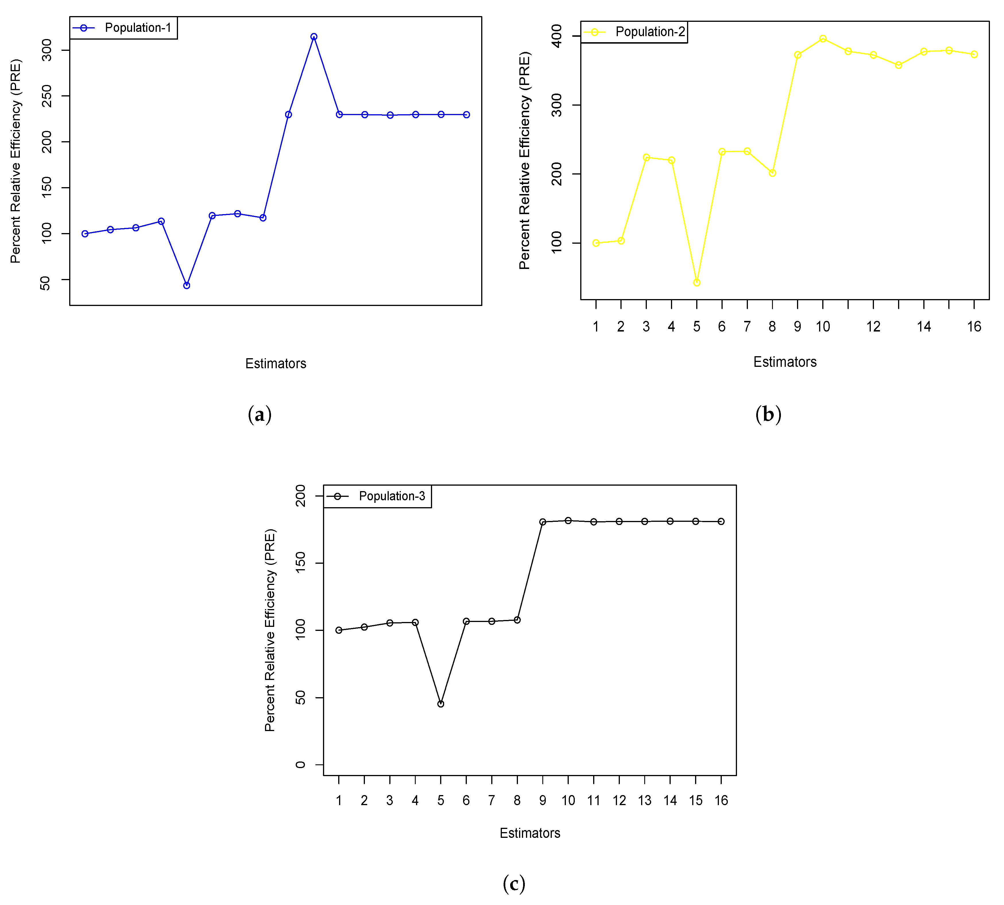
• Additionally, the upward trend in the graphical representations shown in Figure 1 and Figure 2, based on various distributions and actual datasets, further confirms that the new estimators consistently achieve higher PRE values than the conventional estimators. The inverse correlation between the PRE values of the new and traditional estimators strengthens the idea that the newly introduced estimators offer a more efficient estimation method.
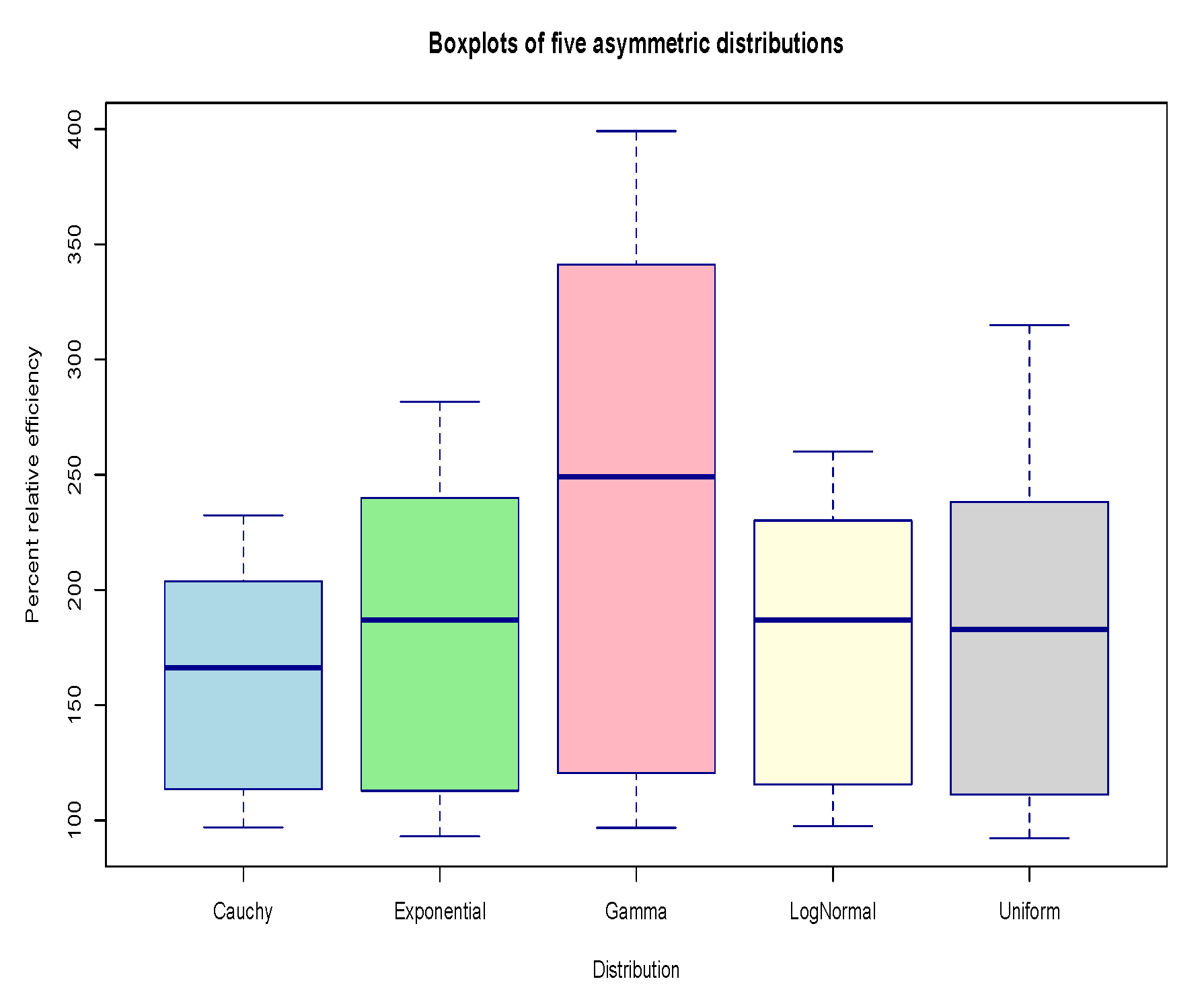
• Furthermore, the box-plots presented in Figure 3 and Figure 4 visually highlight the superior performance of the proposed estimators. These plots display the distribution of percent relative efficiency (PRE) values across both simulated and real datasets, highlighting the consistently higher central tendency and narrower spread of the proposed estimators compared to traditional methods. The compact interquartile ranges and elevated median lines observed in the proposed estimator boxplots signify both robustness and efficiency, particularly under asymmetric and skewed distributions.

7. Conclusions

This study introduces a novel family of estimators for estimating the finite population median under stratified random sampling by utilizing the robust measures of an auxiliary variable. The first-order approximation served as a useful framework for deriving bias and mean-squared error expressions for both existing and newly proposed estimators. This methodology provides deeper insights into their performance and identifies areas for enhancement. To evaluate the effectiveness of the proposed estimators, simulations were conducted using five different distributions under various conditions, along with an analysis of three real-world datasets. The results, summarized in Table 4 and Table 3, indicate that the newly developed estimators demonstrate superior performance and achieve optimal efficiency compared to conventional estimators. Furthermore, all new estimators exhibited higher efficiency than their existing counterparts.

Based on the simulation results and real-life data analysis, the proposed transformation-based estimators $({\widehat{\Omega }}_{e_{1st}},{\widehat{\Omega }}_{e_{2st}},\dots ,{\widehat{\Omega }}_{e_{8st}})$ consistently outperformed the traditional estimators. These estimators achieved the highest percent relative efficiency (PRE) values across various distributions and correlation levels, demonstrating superior accuracy, robustness to skewness, and resistance to outliers.

This study provides a foundation for advancing median estimation within the framework of simple random sampling. Future research may focus on applying the proposed estimators to more complex sampling methods like systematic or two-phase sampling. There is also potential to explore their use in large-scale, high-dimensional datasets and incorporate machine learning techniques to enhance robustness. Furthermore, practical applications, such as healthcare, where accurate median estimates are essential for patient outcomes, and economics, where they are vital for assessing income distribution, can benefit from these improvements. Additionally, developing adaptive methods that automatically select the most suitable estimator based on data characteristics may further enhance accuracy.

In future developments, machine learning techniques could play a significant role in improving estimator performance. For example, supervised algorithms may be utilized to identify transformation rules that minimize estimation error, while unsupervised methods could assist in determining optimal stratum partitions based on underlying data patterns. These adaptive strategies can enhance the flexibility of the proposed estimators, especially in situations involving complex or high-dimensional datasets. Applying such data-driven tools may lead to more efficient and robust median estimation procedures.

References

1. Gross, S. Median estimation in sample surveys. In Proceedings of the Section on Survey Research Methods; American Statistical Association Ithaca, Alexandria, VA, USA; 1980. [Google Scholar]
2. Sedransk, J.; Meyer, J. Confidence intervals for the quantiles of a finite population: Simple random and stratified simple random sampling. J. R. Stat. Soc. Ser. B (Methodol.) 1978, 40, 239–252. [Google Scholar] [CrossRef]
3. Philip, S.; Sedransk, J. Lower bounds for confidence coefficients for confidence intervals for finite population quantiles. Commun. Stat.-Theory Methods 1983, 12, 1329–1344. [Google Scholar] [CrossRef]
4. Kuk, Y.C.A.; Mak, T.K. Median estimation in the presence of auxiliary information. J. R. Stat. Soc. Ser. B 1989, 51, 261–269. [Google Scholar] [CrossRef]
5. Zaman, T.; Bulut, H. An efficient family of robust-type estimators for the population variance in simple and stratified random sampling. Commun. Stat.-Theory Methods 2023, 52, 2610–2624. [Google Scholar] [CrossRef]
6. Daraz, U.; Alomair, M.A.; Albalawi, O.; Al Naim, A.S. New techniques for estimating finite population variance using ranks of auxiliary variable in two-stage sampling. Mathematics 2024, 12, 2741. [Google Scholar] [CrossRef]
7. Alghamdi, A.S.; Alrweili, H. A comparative study of new ratio-type family of estimators under stratified two-phase sampling. Mathematics 2025, 13, 327. [Google Scholar] [CrossRef]
8. Alomair, M.A.; Daraz, U. Dual transformation of auxiliary variables by using outliers in stratified random sampling. Mathematics 2024, 12, 2839. [Google Scholar] [CrossRef]
9. Alghamdi, A.S.; Almulhim, F.A. Optimizing finite population mean estimation using simulation and empirical data. Mathematics 2025, 13, 1635. [Google Scholar] [CrossRef]
10. Rao, T.J. On certail methods of improving ration and regression estimators. Commun. -Stat.-Theory Methods 1991, 20, 3325–3340. [Google Scholar] [CrossRef]
11. Khoshnevisan, M.; Singh, H.P.; Singh, S.; Smarandache, F. A General Class of Estimators of Population Median Using Two Auxiliary Variables in Double Sampling; VirginiaPolytechnic Institute and State University: Blacksburg, VA, USA,, 2002. [Google Scholar]
12. Singh, S.; Joarder, A.H.; Tracy, D.S. Median estimation using double sampling. Aust. N. Z. J. Stat. 2001, 43, 33–46. [Google Scholar] [CrossRef]
13. Singh, S. Advanced Sampling Theory With Applications: How Michael Selected Amy; Springer Science & Business Media: Berlin, Germany, 2003; Volume 2. [Google Scholar]
14. Gupta, S.; Shabbir, J.; Ahmad, S. Estimation of median in two-phase sampling using two auxiliary variables. Commun. Stat.-Theory Methods 2008, 37, 1815–1822. [Google Scholar] [CrossRef]
15. Aladag, S.; Cingi, H. Improvement in estimating the population median in simple random sampling and stratified random sampling using auxiliary information. Commun. Stat.-Theory Methods 2015, 44, 1013–1032. [Google Scholar] [CrossRef]
16. Solanki, R.S.; Singh, H.P. Some classes of estimators for median estimation in survey sampling. Commun. Stat.-Theory Methods 2015, 44, 1450–1465. [Google Scholar] [CrossRef]
17. Daraz, U.; Wu, J.; Albalawi, O. Double exponential ratio estimator of a finite population variance under extreme values in simple random sampling. Mathematics 2024, 12, 1737. [Google Scholar] [CrossRef]
18. Daraz, U.; Wu, J.; Alomair, M.A.; Aldoghan, L.A. New classes of difference cum-ratio-type exponential estimators for a finite population variance in stratified random sampling. Heliyon 2024, 10, e33402. [Google Scholar] [CrossRef]
19. Daraz, U.; Alomair, M.A.; Albalawi, O. Variance estimation under some transformation for both symmetric and asymmetric data. Symmetry 2024, 16, 957. [Google Scholar] [CrossRef]
20. Almulhim, F.A.; Alghamdi, A.S. Simulation-based evaluation of robust transformation techniques for median estimation under simple random sampling. Axioms 2025, 14, 301. [Google Scholar] [CrossRef]
21. Daraz, U.; Almulhim, F.A.; Alomair, M.A.; Alomair, A.M. Population median estimation using auxiliary variables: A simulation study with real data across sample sizes and parameters. Mathematics 2025, 13, 1660. [Google Scholar] [CrossRef]
22. Hussain, M.A.; Javed, M.; Zohaib, M.; Shongwe, S.C.; Awais, M.; Zaagan, A.A.; Irfan, M. Estimation of population median using bivariate auxiliary information in simple random sampling. Heliyon 2024, 10, e28891. [Google Scholar] [CrossRef]
23. Shabbir, J.; Gupta, S. A generalized class of difference type estimators for population median in survey sampling. Hacet. J. Math. Stat. 2017, 46, 1015–1028. [Google Scholar] [CrossRef]
24. Irfan, M.; Maria, J.; Shongwe, S.C.; Zohaib, M.; Bhatti, S.H. Estimation of population median under robust measures of an auxiliary variable. Math. Probl. Eng. 2021, 2021, 4839077. [Google Scholar] [CrossRef]
25. Shabbir, J.; Gupta, S.; Narjis, G. On improved class of difference type estimators for population median in survey sampling. Commun. Stat.-Theory Methods 2022, 51, 3334–3354. [Google Scholar] [CrossRef]
26. Subzar, M.; Lone, S.A.; Ekpenyong, E.J.; Salam, A.; Aslam, M.; Raja, T.A.; Almutlak, S.A. Efficient class of ratio cum median estimators for estimating the population median. PLoS ONE 2023, 18, e0274690. [Google Scholar] [CrossRef] [PubMed]
27. Iseh, M.J. Model formulation on efficiency for median estimation under a fixed cost in survey sampling. Model Assist. Stat. Appl. 2023, 18, 373–385. [Google Scholar] [CrossRef]
28. Shahzad, U.; Ahmad, I.; Alshahrani, F.; Almanjahie, I.M.; Iftikhar, S. Calibration-based mean estimators under stratified median ranked set sampling. Mathematics 2023, 11, 1825. [Google Scholar] [CrossRef]
29. Bhushan, S.; Kumar, A.; Lone, S.A.; Anwar, S.; Gunaime, N.M. An efficient class of estimators in stratified random sampling with an application to real data. Axioms 2023, 12, 576. [Google Scholar] [CrossRef]
30. Alghamdi, A.S.; Alrweili, H. New class of estimators for finite population mean under stratified double phase sampling with simulation and real-life application. Mathematics 2025, 13, 329. [Google Scholar] [CrossRef]
31. Bahl, S.; Tuteja, R. Ratio and product type exponential estimators. J. Inf. Optim. Sci. 1991, 12, 159–164. [Google Scholar] [CrossRef]
32. Daraz, U.; Shabbir, J.; Khan, H. Estimation of finite population mean by using minimum and maximum values in stratified random sampling. J. Mod. Appl. Stat. Methods 2018, 17, 20. [Google Scholar] [CrossRef]
33. Daraz, U.; Khan, M. Estimation of variance of the difference-cum-ratio-type exponential estimator in simple random sampling. Res. Math. Stat. 2021, 8, 1899402. [Google Scholar] [CrossRef]
34. Daraz, U.; Agustiana, D.; Wu, J.; Emam, W. Twofold auxiliary information under two-phase sampling: An improved family of double-transformed variance estimators. Axioms 2025, 14, 64. [Google Scholar] [CrossRef]
35. Daraz, U.; Wu, J.; Agustiana, D.; Emam, W. Finite population variance estimation using Monte Carlo simulation and real life application. Symmetry 2025, 17, 84. [Google Scholar] [CrossRef]
36. Bureau of Statistics. Punjab Development Statistics Government of the Punjab, Lahore, Pakistan; Bureau of Statistics: Islamabad, Pakistan, 2013. [Google Scholar]
37. Bureau of Statistics. Punjab Development Statistics Government of the Punjab, Lahore, Pakistan; Bureau of Statistics: Islamabad, Pakistan, 2014. [Google Scholar]
Figure 1. A visual representation of the results using data collected from various population distributions.
Symmetry 17 01127 g001
Figure 2. A visual representation of the results using data collected from three actual populations. (a) (Source: [13]). (b) (Source: [36]). (c) (Source: [37]).
Symmetry 17 01127 g002
Figure 3. A graphical representation of the percent relative efficiency (PRE) values for various estimators obtained from different artificial populations.
Symmetry 17 01127 g003
Figure 4. A graphical representation of the percent relative efficiency (PRE) values for various estimators obtained from different real populations.
Symmetry 17 01127 g004