Symmetries, Conservation Laws, and Exact Solutions of a Potential Kadomtsev–Petviashvili Equation with Power-Law Nonlinearity

Abstract

This study investigates the potential Kadomtsev–Petviashvili equation incorporating a power-type nonlinearity (PKPp), a model that features prominently in various nonlinear phenomena encountered in physics and applied mathematics. A complete Noether symmetry classification of the PKPp equation is conducted, revealing four distinct scenarios based on different values of the exponent $p$, namely, the general case where $p\ne 1,-1,-2,$ and three special cases where $p=1,$$p=-1,$ and $p=-2.$ Corresponding to each case, conservation laws are derived through a second-order Lagrangian framework. Furthermore, Lie group analysis is employed to reduce the nonlinear partial differential Equation (NLPDE) to ordinary differential Equations (ODEs), thereby enabling the effective application of the Kudryashov method and direct integration techniques to construct exact solutions. In particular, exact solutions of of the considered nonlinear partial differential equation are obtained for the cases $p=1$ and $p=2,$ illustrating the practical implementation of the proposed approach. The solutions obtained include solitary wave, periodic, and rational-type solutions. These results enhance the analytical understanding of the PKPp equation and contribute to the broader theory of nonlinear dispersive equations.

1. Introduction

Recent advances in the theory of nonlinear partial differential equations (NLPDEs) have underscored the importance of exact solutions and soliton dynamics in understanding complex physical systems. For instance, Tian et al. [1] reported a novel long-range instability phenomenon in the inhomogeneous linear Schrödinger equation on the vacuum spacetime quarter-plane, using the linear Fokas unified transform method. Wu and Tian [2] constructed new Hamiltonians with analyzable recursion operators and derived integrability and stability results for smooth multi-solitons of the Dullin–Gottwald–Holm equation. Furthermore, the stability of exact multi-soliton solutions for the two-component Camassa–Holm system was established using bi-Hamiltonian structures and Lyapunov functionals [3].

Significant progress has been made in studying nonlinear wave equations, particularly those admitting exact solitonary solutions. For example, the work by Ankur and Jiwari [4] has provided a detailed account of analytical and numerical methods to understand complex wave structures. Similarly, the study by Kumar and colleagues [5] has demonstrated the power of symmetry methods and integrability techniques in analyzing nonlinear evolution equations with variable coefficients.

Inspired by these developments, this work turns attention to a different but related nonlinear wave equation. The well known Korteweg–de Vries (KdV) equation, initially introduced by Boussinesq [6], models the dynamics of solitary waves, particularly in shallow water with long wavelength and small amplitude. Its two-dimensional extension, known as the Kadomtsev–Petviashvili (KP) equation, was developed by Kadomtsev and Petviashvili [7]. Over the years, the KP equation and its variants have attracted considerable attention in mathematical physics and nonlinear wave theory [8,9]. The (2+1)-dimensional potential Kadomtsev–Petviashvili (PKP) equation

$${\displaystyle {\varphi }_{tx}+\frac{3}{2}{\varphi }_x{\varphi }_{xx}+\frac{1}{4}{\varphi }_{xxxx}+\frac{3}{4}{\varphi }_{yy}=0}$$

(1)

has been the focus of numerous studies aimed at exploring its rich mathematical structure and exact solutions [10,11,12,13,14,15,16,17,18]. For example, Humbu et al. [13] used a variety of wave ansatz methods to extract bright, singular, shock waves also referred to as dark or topological or kink soliton solutions while Kaya and El-Sayed [15] applied the Adomian decomposition method to obtain numerical soliton-like solutions, and Li and Zhang [16], amongst many other authors who have studied this equation, enhanced the homogeneous balance method to derive various types of solutions.

While the standard KP and its potential forms have been studied extensively for their integrability and soliton dynamics [7,19], relatively fewer works address the potential KP equation with generalized power-law nonlinearities. Studies by Wang and Chen [20], for example, introduce power-law modifications to KP-type models but do not explore the associated symmetry structures in depth. The symmetry and conservation law analysis of such generalized systems remains largely underdeveloped. Advances in symmetry analysis [21,22] and conservation law derivation methods [23] offer robust frameworks to fill this gap. Therefore, this paper aims to systematically investigate the symmetries, conservation laws, and exact solutions of the potential KP equation with arbitrary power-law nonlinearity, a direction that has not been comprehensively explored in the existing literature.

A generalization of the PKP equation includes power-law nonlinearity, leading to the PKPp equation,

$${\varphi }_{tx}+\alpha {\varphi }_x^p{\varphi }_{xx}+\beta {\varphi }_{xxxx}-\gamma {\varphi }_{yy}=0,$$

(2)

where $\alpha ,\beta ,\gamma$, and p are non-zero constants [24].

This form of the equation allows for richer nonlinear dynamics and has recently been studied for specific values of p. The generalization introduced in Equation (2) serves to explore a broader class of nonlinear evolution equations by incorporating power-law nonlinearity through the term ${\varphi }_x^p{\varphi }_{xx}.$ This type of generalization is common in nonlinear science, as it allows for the modeling of more complex physical phenomena where the nonlinear effect depends on the spatial gradient raised to a power. Such formulations can better capture features like steepening waves, nonuniform dispersion, or anomalous transport.

The chosen form is motivated by physical relevance and mathematical tractability. The term ${\varphi }_x^p{\varphi }_{xx}$ maintains the balance between nonlinearity and dispersion in a way that is consistent with known integrable systems and allows for the construction of exact solutions using analytical techniques such as similarity reductions or the Lie symmetry method. Moreover, this structure appears in generalized fluid dynamics and plasma models, lending further justification to its adoption in this context. Gupta and Bansal [25] explored the (2+1)-dimensional variable coefficient potential Kadomtsev–Petviashvili (VCPKP) equation,

$$u_{tx}+\alpha \left(t\right)u_x{u}_{xx}+\beta \left(t\right)u_{xxxx}+\delta \left(t\right)u_{yy}=0,$$

(3)

where $\alpha \left(t\right)$, $\beta \left(t\right)$, and $\delta \left(t\right)$ are arbitrary time-dependent functions but sufficiently smooth functions of time. $\alpha \left(t\right)$, $\beta \left(t\right)$, $\delta \left(t\right)\in C^1(\Re ),$ meaning that they are continuously differentiable on $\Re .$ This level of smoothness ensures the applicability of analytical techniques such as symmetry analysis and the derivation of conservation laws, and it also guarantees the mathematical consistency and well-posedness of the governing equation. They investigated the integrability of the equation and derived exact solutions by applying methods and techniques similar to those used in [26], ultimately obtaining a range of general solutions for the VCPKP equation. Recently, Sebogodi, Muatjetjeja, and Adem [27] investigated a related combined potential Kadomtsev–Petviashvili-B-type KP equation using Lie symmetry analysis. Their work yielded new exact solutions and conservation laws, contributing significantly to the understanding of (2+1)-dimensional NLPDEs. Their approach provides a strong foundation for the methods applied in the present study.

Moreover, several recent studies have employed Lie group methods, Noether symmetry classification, and Kudryashov’s method to derive exact solutions for generalized KP-type equations with variable coefficients or nonlinearities of the form $u^p.$ For example, Afolabi and Johnpillai applied Lie symmetry and KM to generalized KP equations with damping and power-law nonlinearities [28], while Alquran and Mahgoub examined wave structures using ansatz techniques for KP-type models [29]. Meanwhile, Umaru and colleagues systematically explored Noether symmetries and conservation laws of higher-order nonlinear evolution Equations [30].

Despite these advancements, there remains a significant gap in the literature on symmetry classifications and exact solutions of the PKPp equation. Most studies either fix specific forms of the nonlinearity or restrict analysis to numerical approaches. Few address how varying the exponent p influences the structure of symmetries, conservation laws, and solution behavior. There is thus a need for a systematic investigation that combines analytical symmetry analysis, conservation law derivation, and closed-form solution techniques across different values of $p.$

This study directly addresses that gap. We perform a Noether symmetry classification of the PKPp equation and derive the associated conservation laws for a range of values of $p,$ where $p\ne 1,-1,-2,$ and three special cases where $p=1,$$p=-1,$ and $p=-2.$ In addition, we apply Lie symmetry analysis to reduce Equation (2) to an ODE in order to use KM and direct integration to obtain exact solutions for the specific cases $p=1$ and $p=2.$ Our results offer new insights into the structural properties of the PKPp equation and contribute to the broader understanding of nonlinear evolution equations in higher dimensions.

2. Conservation Laws Associated with Equation (2)

The vector field

$$\begin{array}{c}\hfill {\displaystyle \Gamma ={\tau }^1(t,x,y,\varphi )\frac{\partial }{\partial t}+{\tau }^2(t,x,y,\varphi )\frac{\partial }{\partial x}+{\tau }^3(t,x,y,\varphi )\frac{\partial }{\partial y}+\eta (t,x,y,\varphi )\frac{\partial }{\partial \varphi }}\end{array}$$

(4)

is referred to as a Noether point symmetry associated with a second-order Lagrangian L corresponding to Equation (2) if the condition

$${\Gamma }^{\left[2\right]}\left(L\right)+\{D_t\left({\tau }^1\right)+D_x\left({\tau }^2\right)+D_y\left({\tau }^3\right)\}L=D_t\left(F^1\right)+D_x\left(F^2\right)+D_y\left(F^3\right)$$

(5)

is satisfied for certain smooth functions $F^1(t,x,y,\varphi )$, $F^2(t,x,y,\varphi )$, and $F^3(t,x,y,\varphi ),$ commonly known as gauge functions.

The second-order prolongation ${\Gamma }^{\left[2\right]}$ is given by

$$\begin{array}{ccc}\hfill {\Gamma }^{\left[2\right]}& =& {\displaystyle {\tau }^1\frac{\partial }{\partial t}+{\tau }^2\frac{\partial }{\partial x}+{\tau }^3\frac{\partial }{\partial y}+\eta \frac{\partial }{\partial \varphi }+{\zeta }_t\frac{\partial }{\partial {\varphi }_t}+}\hfill \\ & & {\displaystyle {\zeta }_x\frac{\partial }{\partial {\varphi }_x}+{\zeta }_{tt}\frac{\partial }{\partial {\varphi }_{tt}}+{\zeta }_{xx}\frac{\partial }{\partial {\varphi }_{xx}}+{\zeta }_{tx}\frac{\partial }{\partial {\varphi }_{tx}}+\dots }\hfill \end{array}$$

where the expressions for ${\zeta }_t,{\zeta }_x,{\zeta }_{tx},{\zeta }_{tt}$, and ${\zeta }_{xx}$ are given in [31]. The total differential operators are given by

$$\begin{array}{ccc}\hfill D_t& =& {\displaystyle \frac{\partial }{\partial t}+{\varphi }_t\frac{\partial }{\partial \varphi }+{\varphi }_{tt}\frac{\partial }{\partial {\varphi }_t}+{\varphi }_{xt}\frac{\partial }{\partial {\varphi }_x}+\dots ,}\hfill \\ \hfill D_x& =& {\displaystyle \frac{\partial }{\partial x}+{\varphi }_x\frac{\partial }{\partial \varphi }+{\varphi }_{xx}\frac{\partial }{\partial {\varphi }_x}+{\varphi }_{xt}\frac{\partial }{\partial {\varphi }_t}+\dots ,}\hfill \\ \hfill D_y& =& {\displaystyle \frac{\partial }{\partial x}+{\varphi }_x\frac{\partial }{\partial \varphi }+{\varphi }_{xx}\frac{\partial }{\partial {\varphi }_x}+{\varphi }_{xt}\frac{\partial }{\partial {\varphi }_t}+\dots .}\hfill \end{array}$$

It is evident that determining the Noether operators for the PKPp Equation (2) requires a separate analysis of four distinct cases.

• Case 1: p is arbitrary but $p\ne 1,-1,-2$

For this case, the corresponding Lagrangian of the PKPp Equation (2) is expressed as

$$\begin{array}{c}\hfill L=-{\displaystyle \frac{1}{2}}{\varphi }_t{\varphi }_x-{\displaystyle \frac{\alpha }{(p+1)(p+2)}}{\varphi }_x^{p+2}+{\displaystyle \frac{\beta }{2}}{\varphi }_{xx}^2+{\displaystyle \frac{\gamma }{2}}{\varphi }_y^2.\end{array}$$

(6)

Substituting this expression for L into Equation (5) results in an overdetermined system consisting of nineteen linear partial differential equations (PDEs). These equations are as follows:

$$\begin{array}{ccc}& & {\tau }_x^1=0,{\tau }_y^1=0,{\tau }_{\varphi }^1=0,{\tau }_t^2=0,{\tau }_{xx}^2=0,{\tau }_{\varphi }^2=0,{\tau }_x^3=0,{\tau }_{\varphi }^3=0,\hfill \\ \hfill & & {\eta }_x=0,{\eta }_{\varphi \varphi }=0,{\eta }_{\varphi }+{\displaystyle \frac{1}{2}}{\tau }_y^3=0,{\displaystyle \frac{1}{2}}{\tau }_t^3-\gamma {\tau }_y^2=0,\gamma {\eta }_y-F_{\varphi }^3=0,\hfill \\ \hfill & & {\displaystyle \frac{1}{2}}{\eta }_t+F_{\varphi }^2=0,\gamma {\eta }_{\varphi }-{\displaystyle \frac{1}{2}}\gamma {\tau }_y^3+{\displaystyle \frac{1}{2}}\gamma {\tau }_x^2+{\displaystyle \frac{1}{2}}\gamma {\tau }_t^1=0,\hfill \\ \hfill & & \beta {\eta }_{\varphi }+{\displaystyle \frac{1}{2}}\beta {\tau }_y^3+{\displaystyle \frac{1}{2}}\beta {\tau }_t^1-{\displaystyle \frac{3}{2}}\beta {\tau }_x^2=0,F_{\varphi }^1=0,F_t^1+F_x^2+F_y^3=0,\hfill \\ \hfill & & {\displaystyle \frac{\alpha }{p+1}}{\eta }_{\varphi }+{\displaystyle \frac{\alpha }{(p+1)(p+2)}}{\tau }_t^1-{\displaystyle \frac{\alpha }{p+2}}{\tau }_x^2+{\displaystyle \frac{\alpha }{(p+1)(p+2)}}{\tau }_y^3=0.\hfill \end{array}$$

The solution of the aforementioned system of PDEs leads to

$$\begin{array}{ccc}\hfill {\tau }^1& =& C_1,\hfill \\ \hfill {\tau }^2& =& C_{2}y+C_3,\hfill \\ \hfill {\tau }^3& =& 2\gamma t{C}_2+C_4,\hfill \\ \hfill \eta & =& yM\left(t\right)+N\left(t\right),\hfill \\ \hfill F^1& =& Q(t,x,y),\hfill \\ \hfill F^2& =& R(t,x,y)-{\displaystyle \frac{1}{2}}\varphi (y{M}^{\prime }\left(t\right)+N^{\prime }\left(t\right)),\hfill \\ \hfill F^3& =& H(t,x,y)+\gamma \varphi M\left(t\right),\hfill \end{array}$$

(7)

where $C_1,C_2,C_3,$ and $C_4$ are constants and $M\left(t\right),N\left(t\right),Q(t,x,y),R(t,x,y)$, and $H(t,x,y)$ are arbitrary functions of their arguments. The associated generic vector fields of the infinitesimal transformations that preserve the invariance of Equation (2), along with their respective gauge functions, are given as follows

$$\begin{array}{ccc}\hfill {\Gamma }_1& =& {\displaystyle \frac{\partial }{\partial t},F^1=F^2=F^3=0,}\hfill \end{array}$$

(8)

$$\begin{array}{ccc}\hfill {\Gamma }_2& =& {\displaystyle \frac{\partial }{\partial x},F^1=F^2=F^3=0,}\hfill \end{array}$$

(9)

$$\begin{array}{ccc}\hfill {\Gamma }_3& =& {\displaystyle \frac{\partial }{\partial y},F^1=F^2=F^3=0,}\hfill \end{array}$$

(10)

$$\begin{array}{ccc}\hfill {\Gamma }_4& =& {\displaystyle y\frac{\partial }{\partial x}+2\gamma t\frac{\partial }{\partial y},F^1=F^2=F^3=0,}\hfill \end{array}$$

(11)

$$\begin{array}{ccc}\hfill {\Gamma }_5& =& {\displaystyle yM\left(t\right)\frac{\partial }{\partial \varphi },F^1=0,F^2=-\frac{1}{2}\varphi y{M}^{\prime }\left(t\right),F^3=\gamma \varphi M\left(t\right),}\hfill \end{array}$$

(12)

$$\begin{array}{ccc}\hfill {\Gamma }_6& =& {\displaystyle N\left(t\right)\frac{\partial }{\partial \varphi },F^1=F^3=0,F^2=-\frac{1}{2}\varphi N^{\prime }\left(t\right).}\hfill \end{array}$$

(13)

By applying Noether’s theorem [32], we derive the six nontrivial conserved vectors corresponding to the Noether point symmetries listed above.

$$\begin{array}{cc}\hfill & {\Omega }_1^1={\displaystyle \frac{1}{2}}\beta {\varphi }_{xx}^2-{\displaystyle \frac{\alpha }{(p+1)(p+2)}}{\varphi }_x^{p+2}+{\displaystyle \frac{1}{2}}\gamma {\varphi }_y^2,\hfill \\ \hfill & {\Omega }_1^2=\beta {\varphi }_t{\varphi }_{xxx}+{\displaystyle \frac{\alpha }{p+1}}{\varphi }_t{\varphi }_x^{p+1}+{\displaystyle \frac{1}{2}}{\varphi }_t^2-\beta {\varphi }_{tx}{\varphi }_{xx},\hfill \\ \hfill & {\Omega }_1^3=-\gamma {\varphi }_t{\varphi }_y;\hfill \end{array}$$

(14)

$$\begin{array}{cc}\hfill & \hfill \\ \hfill & {\Omega }_2^1={\displaystyle \frac{1}{2}}{\varphi }_x^2,\hfill \\ \hfill & {\Omega }_2^2=\beta {\varphi }_x{\varphi }_{xxx}-{\displaystyle \frac{1}{2}}\beta {\varphi }_{xx}^2+{\displaystyle \frac{1}{2}}\gamma {\varphi }_y^2+{\displaystyle \frac{\alpha }{p+2}}{\varphi }_x^{p+2},\hfill \\ \hfill & {\Omega }_2^3=-\gamma {\varphi }_x{\varphi }_y;\hfill \end{array}$$

(15)

$$\begin{array}{cc}\hfill & \hfill \\ \hfill & {\Omega }_3^1={\displaystyle \frac{1}{2}}{\varphi }_x{\varphi }_y,\hfill \\ \hfill & {\Omega }_3^2={\displaystyle \frac{1}{2}}{\varphi }_t{\varphi }_y+{\displaystyle \frac{\alpha }{p+1}}{\varphi }_x^{p+1}{\varphi }_y+\beta {\varphi }_y{\varphi }_{xxx}-\beta {\varphi }_{xy}{\varphi }_{xx},\hfill \\ \hfill & {\Omega }_3^3=-{\displaystyle \frac{1}{2}}{\varphi }_t{\varphi }_x-{\displaystyle \frac{\alpha }{(p+1)(p+2)}}{\varphi }_x^{p+2}+{\displaystyle \frac{1}{2}}\beta {\varphi }_{xx}^2-{\displaystyle \frac{1}{2}}\gamma {\varphi }_y^2;\hfill \end{array}$$

(16)

$$\begin{array}{cc}\hfill & \hfill \\ \hfill & {\Omega }_4^1={\displaystyle \frac{1}{2}}y{\varphi }_x^2+\gamma t{\varphi }_x{\varphi }_y,\hfill \\ \hfill & {\Omega }_4^2=\beta y{\varphi }_x{\varphi }_{xxx}+2\gamma \beta t{\varphi }_y{\varphi }_{xxx}+{\displaystyle \frac{1}{2}}\gamma y{\varphi }_y^2+\gamma t{\varphi }_t{\varphi }_y-{\displaystyle \frac{1}{2}}\beta y{\varphi }_{xx}^2\hfill \\ \hfill & +{\displaystyle \frac{\alpha }{p+1}}y{\varphi }_x^{p+2}+{\displaystyle \frac{2\alpha \gamma }{p+1}}t{\varphi }_y{\varphi }_x^{p+1}-2\beta \gamma t{\varphi }_{xy}{\varphi }_{xx},\hfill \\ \hfill & {\Omega }_4^3=\beta \gamma t{\varphi }_{xx}^2-{\gamma }^{2}t{\varphi }_y^2-\gamma y{\varphi }_x{\varphi }_y-\gamma t{\varphi }_t{\varphi }_x-{\displaystyle \frac{2\alpha \gamma }{(p+1)(p+2)}}t{\varphi }_x^{p+2};\hfill \end{array}$$

(17)

$$\begin{array}{cc}\hfill & {\Omega }_5^1=-{\displaystyle \frac{1}{2}}yM\left(t\right){\varphi }_x,\hfill \\ \hfill & {\Omega }_5^2=-{\displaystyle \frac{1}{2}}yM\left(t\right){\varphi }_t-{\displaystyle \frac{\alpha }{p+1}}yM\left(t\right){\varphi }_x^{p+1}-\beta yM\left(t\right){\varphi }_{xxx}+{\displaystyle \frac{1}{2}}\varphi y{M}^{\prime }\left(t\right),\hfill \\ \hfill & {\Omega }_5^3=\gamma yM\left(t\right){\varphi }_y-\lambda \varphi M\left(t\right);\hfill \end{array}$$

(18)

$$\begin{array}{cc}\hfill & \hfill \\ \hfill & {\Omega }_6^1=-{\displaystyle \frac{1}{2}}{\varphi }_{x}N\left(t\right),\hfill \\ \hfill & {\Omega }_6^2=-{\displaystyle \frac{1}{2}}{\varphi }_{t}N\left(t\right)-{\displaystyle \frac{\alpha }{p+1}}{\varphi }_x^{p+1}N\left(t\right)-\beta {\varphi }_{xxx}N\left(t\right)+{\displaystyle \frac{1}{2}}\varphi N^{\prime }\left(t\right),\hfill \\ \hfill & {\Omega }_6^3=\gamma {\varphi }_{y}N\left(t\right).\hfill \end{array}$$

(19)

• Case 2:$p=1$

When $p=1$, the PKPp Equation (2) becomes

$$\begin{array}{c}\hfill {\varphi }_{tx}+\alpha {\varphi }_x{\varphi }_{xx}+\beta {\varphi }_{xxxx}-\gamma {\varphi }_{yy}=0.\end{array}$$

(20)

It is observed that Equation (20) admits a Lagrangian formulation with the associated Lagrangian given by

$$L=-{\displaystyle \frac{1}{2}}{\varphi }_t{\varphi }_x-{\displaystyle \frac{1}{6}}\alpha {\varphi }_x^3+{\displaystyle \frac{1}{2}}\beta {\varphi }_{xx}^2+{\displaystyle \frac{1}{2}}\gamma {\varphi }_y^2.$$

(21)

By applying the same procedure as in Case 1, we derive ten Noether symmetries. The first four, ${\Gamma }_1,,{\Gamma }_2,{\Gamma }_3,$ and ${\Gamma }_4$, are presented in Equations (8)–(11), while the remaining six are listed below,

$$\begin{array}{ccc}\hfill {\Gamma }_5& =& {\displaystyle y\frac{\partial }{\partial \varphi },F^1=F^2=0,F^3=\gamma \varphi ,}\hfill \end{array}$$

(22)

$$\begin{array}{ccc}\hfill {\Gamma }_6& =& {\displaystyle \alpha t\frac{\partial }{\partial x}+x\frac{\partial }{\partial \varphi },F^1=-\frac{1}{2}\varphi ,F^2=F^3=0,}\hfill \end{array}$$

(23)

$$\begin{array}{ccc}\hfill {\Gamma }_7& =& {\displaystyle \frac{1}{2}\alpha t^2\frac{\partial }{\partial x}+(xt+\frac{1}{2\gamma }{y}^2)\frac{\partial }{\partial \varphi },F^1=-\frac{1}{2}\varphi t,}\hfill \\ & & F^2=-{\displaystyle \frac{1}{2}}\varphi x,F^3=y\varphi ,\hfill \end{array}$$

(24)

$$\begin{array}{ccc}\hfill {\Gamma }_8& =& {\displaystyle \alpha yt\frac{\partial }{\partial x}+\alpha \gamma t^2\frac{\partial }{\partial y}+xy\frac{\partial }{\partial \varphi },F^1=-\frac{1}{2}\varphi y,}\hfill \\ & & F^2=0,F^3=\gamma \varphi x,\hfill \end{array}$$

(25)

$$\begin{array}{ccc}\hfill {\Gamma }_9& =& {\displaystyle \frac{1}{2}\alpha y{t}^2\frac{\partial }{\partial x}+\frac{1}{3}\alpha \gamma t^3\frac{\partial }{\partial y}+(xty+\frac{1}{6\gamma }{y}^3)\frac{\partial }{\partial \varphi },}\hfill \\ & & F^1=-{\displaystyle \frac{1}{2}}\varphi ty;F^2=-{\displaystyle \frac{1}{2}}\varphi xy;F^3=\gamma \varphi xt+{\displaystyle \frac{1}{2}}\varphi y^2,\hfill \end{array}$$

(26)

$$\begin{array}{ccc}\hfill {\Gamma }_{10}& =& {\displaystyle 3t\frac{\partial }{\partial t}+x\frac{\partial }{\partial x}+2y\frac{\partial }{\partial y}-\varphi \frac{\partial }{\partial \varphi },F^1=F^2=F^3=0.}\hfill \end{array}$$

(27)

By applying Noether’s theorem [32], a total of ten conserved quantities are derived. The first four arise from the symmetry generators (8)–(11) and are explicitly expressed in Equations (14)–(17) for the case $p=1.$ The remaining six conserved vectors correspond to the generators (22)–(27) and are presented as follows:

$$\begin{array}{cc}\hfill & {\Omega }_5^1={\displaystyle \frac{1}{2}}y{\varphi }_x,\hfill \\ \hfill & {\Omega }_5^2={\displaystyle \frac{1}{2}}y{\varphi }_t+{\displaystyle \frac{1}{2}}\alpha y{\varphi }_x^2+\beta y{\varphi }_{xxx},\hfill \\ \hfill & {\Omega }_5^3=\gamma \varphi -\gamma y{\varphi }_y;\hfill \end{array}$$

(28)

$$\begin{array}{cc}\hfill & \hfill \\ \hfill & {\Omega }_6^1={\displaystyle \frac{1}{2}}\alpha t{\varphi }_x^2-{\displaystyle \frac{1}{2}}x{\varphi }_x+{\displaystyle \frac{1}{2}}\varphi ,\hfill \\ \hfill & {\Omega }_6^2=\alpha \beta t{\varphi }_x{\varphi }_{xxx}-\beta x{\varphi }_{xxx}+\beta {\varphi }_{xx}+{\displaystyle \frac{1}{3}}{\alpha }^{2}t{\varphi }_x^3-{\displaystyle \frac{1}{2}}\alpha \beta t{\varphi }_{xx}^2\hfill \\ & +{\displaystyle \frac{1}{2}}\alpha \gamma y{\varphi }_y^2-{\displaystyle \frac{1}{2}}x{\varphi }_t-{\displaystyle \frac{1}{2}}\alpha x{\varphi }_x^2,\hfill \\ \hfill & {\Omega }_6^3=\gamma x{\varphi }_y-\alpha \gamma t{\varphi }_x{\varphi }_y;\hfill \end{array}$$

(29)

$$\begin{array}{cc}\hfill & \hfill \\ \hfill & {\Omega }_7^1={\displaystyle \frac{1}{4}}\alpha t^2{\varphi }_x^2-{\displaystyle \frac{1}{2}}xt{\varphi }_x-{\displaystyle \frac{1}{4\gamma }}{y}^2{\varphi }_x+{\displaystyle \frac{1}{2}}\varphi t,\hfill \\ \hfill & {\Omega }_7^2={\displaystyle \frac{1}{6}}{\alpha }^2{t}^2{\varphi }_x^3-{\displaystyle \frac{1}{4}}\alpha \beta t^2{\varphi }_{xx}^2+{\displaystyle \frac{1}{4}}\alpha \gamma t^2{\varphi }_y^2-{\displaystyle \frac{1}{2}}xt{\varphi }_t-{\displaystyle \frac{1}{2}}\alpha xt{\varphi }_x^2\hfill \\ & -\beta xt{\varphi }_{xxx}-{\displaystyle \frac{1}{4\gamma }}{y}^2{\varphi }_t-{\displaystyle \frac{1}{4\gamma }}\alpha y^2{\varphi }_x^2-{\displaystyle \frac{1}{2\gamma }}\beta y^2{\varphi }_{xxx}+{\displaystyle \frac{1}{2}}\alpha \beta t^2{\varphi }_{xxx}\hfill \\ & +\beta t{\varphi }_{xx}+{\displaystyle \frac{1}{2}}\varphi x,\hfill \\ \hfill & {\Omega }_7^3=\gamma xt{\varphi }_y+{\displaystyle \frac{1}{2}}{y}^2{\varphi }_y-{\displaystyle \frac{1}{2}}\alpha \gamma t^2{\varphi }_x{\varphi }_y-y\varphi ;\hfill \end{array}$$

(30)

$$\begin{array}{cc}\hfill & \hfill \\ \hfill & {\Omega }_8^1={\displaystyle \frac{1}{2}}\alpha \gamma t^2{\varphi }_x{\varphi }_y+{\displaystyle \frac{1}{2}}\alpha yt{\varphi }_x^2-{\displaystyle \frac{1}{2}}xy{\varphi }_x+{\displaystyle \frac{1}{2}}y\varphi ,\hfill \\ \hfill & {\Omega }_8^2={\displaystyle \frac{1}{3}}{\alpha }^{2}yt{\varphi }_x^3-{\displaystyle \frac{1}{2}}\alpha \beta yt{\varphi }_{xx}^2+{\displaystyle \frac{1}{2}}\alpha \gamma yt{\varphi }_y^2-{\displaystyle \frac{1}{2}}xy{\varphi }_t-{\displaystyle \frac{1}{2}}\alpha xy{\varphi }_x^2\hfill \\ & -\beta xy{\varphi }_{xxx}+\alpha \beta yy{\varphi }_x{\varphi }_{xxx}+{\displaystyle \frac{1}{2\alpha \gamma }}{t}^2{\varphi }_t{\varphi }_y+{\displaystyle \frac{1}{2}}{\alpha }^2\gamma t^2{\varphi }_x^2{\varphi }_y\hfill \\ & +\alpha \beta \gamma t^2{\varphi }_y{\varphi }_{xxx}+\beta y{\varphi }_{xx}-\alpha \beta \gamma t^2{\varphi }_{xx}{\varphi }_{xy},\hfill \\ \hfill & {\Omega }_8^3={\displaystyle \frac{1}{2}}\alpha \beta \gamma t^2{\varphi }_{xx}^2-{\displaystyle \frac{1}{2}}\alpha \gamma t^2{\varphi }_t{\varphi }_x-{\displaystyle \frac{1}{6}}{\alpha }^2\gamma t^2{\varphi }_x^3-{\displaystyle \frac{1}{2}}\alpha {\gamma }^2{t}^2{\varphi }_y^2\hfill \\ & +\gamma xy{\varphi }_y-\alpha \gamma yt{\varphi }_x{\varphi }_y-\gamma x\varphi ;\hfill \end{array}$$

(31)

$$\begin{array}{cc}\hfill & \hfill \\ \hfill & {\Omega }_9^1={\displaystyle \frac{1}{6}}\alpha \gamma t^3{\varphi }_x{\varphi }_y+{\displaystyle \frac{1}{4}}\alpha y{t}^2{\varphi }_x^2-{\displaystyle \frac{1}{12\gamma }}{y}^3{\varphi }_x-{\displaystyle \frac{1}{2}}xyt+{\displaystyle \frac{1}{2}}yt\varphi ,\hfill \\ \hfill & {\Omega }_9^2={\displaystyle \frac{1}{6}}{\alpha }^{2}y{t}^2{\varphi }_x^3-{\displaystyle \frac{1}{4}}\alpha \beta y{t}^2{\varphi }_{xx}^2+{\displaystyle \frac{1}{4}}\alpha \gamma y{t}^2{\varphi }_y^2-{\displaystyle \frac{1}{2}}xy{\varphi }_t-{\displaystyle \frac{1}{2}}\alpha xyt{\varphi }_x^2\hfill \\ & -\beta xyt{\varphi }_{xxx}-{\displaystyle \frac{1}{12\gamma }}{y}^3{\varphi }_t-{\displaystyle \frac{1}{12\gamma }}\alpha y^3{\varphi }_x^2-{\displaystyle \frac{1}{6\gamma }}\beta y^3{\varphi }_{xxx}+{\displaystyle \frac{1}{2}}\alpha \beta y{t}^2{\varphi }_x{\varphi }_{xxx}\hfill \\ & +{\displaystyle \frac{1}{6}}\alpha \gamma t^3{\varphi }_t{\varphi }_y+{\displaystyle \frac{1}{6}}{\alpha }^2\gamma t^3{\varphi }_x^2{\varphi }_y+{\displaystyle \frac{1}{3}}\alpha \beta \gamma t^3{\varphi }_y{\varphi }_{xxx}+\beta ty{\varphi }_{xx}\hfill \\ & -{\displaystyle \frac{1}{3}}\alpha \beta \gamma t^3{\varphi }_{xx}{\varphi }_{xy}+{\displaystyle \frac{1}{2}}xy\varphi ,\hfill \\ \hfill & {\Omega }_9^3={\displaystyle \frac{1}{6}}\alpha \beta \gamma t^3{\varphi }_{xx}^2-{\displaystyle \frac{1}{6}}\alpha \gamma t^3{\varphi }_t{\varphi }_x-{\displaystyle \frac{1}{18}}{\alpha }^2\gamma t^3{\varphi }_x^3-{\displaystyle \frac{1}{6}}\alpha {\gamma }^2{t}^3{\varphi }_y^2\hfill \\ & +\gamma txy{\varphi }_y+{\displaystyle \frac{1}{6}}{y}^3{\varphi }_y-{\displaystyle \frac{1}{2}}\alpha \gamma y{t}^2{\varphi }_x{\varphi }_y-\gamma tx\varphi -{\displaystyle \frac{1}{2}}{y}^2\varphi ;\hfill \end{array}$$

(32)

$$\begin{array}{cc}\hfill & {\Omega }_{10}^1={\displaystyle \frac{3}{2}}\beta t{\varphi }_{xx}-{\displaystyle \frac{1}{2}}\alpha t{\varphi }_x^3+{\displaystyle \frac{3}{2}}\gamma t{\varphi }_y^2+{\displaystyle \frac{1}{2}}\varphi {\varphi }_x+{\displaystyle \frac{1}{2}}x{\varphi }_x^2+y{\varphi }_x{\varphi }_y,\hfill \\ \hfill & {\Omega }_{10}^2={\displaystyle \frac{1}{3}}\alpha x{\varphi }_x^3-{\displaystyle \frac{1}{2}}\beta x{\varphi }_{xx}^2+{\displaystyle \frac{1}{2}}\gamma x{\varphi }_y^2+{\displaystyle \frac{1}{2}}\varphi {\varphi }_t+{\displaystyle \frac{1}{2}}\alpha \varphi {\varphi }_x^2+\beta \varphi {\varphi }_{xxx}\hfill \\ & +{\displaystyle \frac{3}{2}}t{\varphi }_t^2+{\displaystyle \frac{3}{2}}\alpha t{\varphi }_t{\varphi }_x^2+3\beta t{\varphi }_t{\varphi }_{xxx}+\beta x{\varphi }_x{\varphi }_{xxx}+y{\varphi }_t{\varphi }_y+\alpha y{\varphi }_x^2{\varphi }_y\hfill \\ & +2\beta y{\varphi }_y{\varphi }_{xxx}-\beta {\varphi }_x{\varphi }_{xx}-3\beta t{\varphi }_{tx}{\varphi }_{xx}-\beta {\varphi }_x{\varphi }_{xx}-2\beta y{\varphi }_{xx}{\varphi }_{xy},\hfill \\ \hfill & {\Omega }_{10}^3=\beta y{\varphi }_{xx}^2-y{\varphi }_t{\varphi }_x-{\displaystyle \frac{1}{3}}\alpha y{\varphi }_x^3-\gamma y{\varphi }_y^2-\gamma \varphi {\varphi }_y-3\gamma t{\varphi }_t{\varphi }_y-\gamma x{\varphi }_x{\varphi }_y.\hfill \end{array}$$

(33)

• Case 3:$p=-1$

We now turn our attention to the case where $p=-1.$ In this case, Equation (2) takes the form

$$\begin{array}{c}\hfill {\varphi }_{tx}+\alpha {\varphi }_x^{-1}{\varphi }_{xx}+\beta {\varphi }_{xxxx}-\gamma {\varphi }_{yy}=0.\end{array}$$

(34)

It is can be verified that Equation (34) admits a Lagrangian

$$L=-{\displaystyle \frac{1}{2}}{\varphi }_t{\varphi }_x-\alpha {\varphi }_{x}ln\left({\varphi }_x\right)+{\displaystyle \frac{1}{2}}\beta {\varphi }_{xx}^2+{\displaystyle \frac{\gamma }{2}}{\varphi }_y^2.$$

(35)

Applying the same procedure as above yields six Noether point symmetries, identical to those found in Case 1. Consequently, the corresponding conserved vectors are given by

$$\begin{array}{cc}\hfill & {\Omega }_1^1={\displaystyle \frac{1}{2}}\gamma {\varphi }_y^2+{\displaystyle \frac{1}{2}}\beta {\varphi }_{xx}^2,\hfill \\ \hfill & {\Omega }_1^2={\displaystyle \frac{1}{2}}{\varphi }_t^2+\alpha {\varphi }_{t}ln\left({\varphi }_x\right)+\alpha {\varphi }_t+\beta {\varphi }_t{\varphi }_{xxx}-\beta {\varphi }_{tx}{\varphi }_{xx},\hfill \\ \hfill & {\Omega }_1^3=-\gamma {\varphi }_t{\varphi }_y;\hfill \end{array}$$

(36)

$$\begin{array}{cc}\hfill & \hfill \\ \hfill & {\Omega }_2^1={\displaystyle \frac{1}{2}}{\varphi }_x^2,\hfill \\ \hfill & {\Omega }_2^2=\beta {\varphi }_x{\varphi }_{xxx}-{\displaystyle \frac{1}{2}}\beta {\varphi }_{xx}^2+{\displaystyle \frac{1}{2}}\gamma {\varphi }_y^2+\alpha {\varphi }_x,\hfill \\ \hfill & {\Omega }_2^3=-\gamma {\varphi }_x{\varphi }_y;\hfill \end{array}$$

(37)

$$\begin{array}{cc}\hfill & \hfill \\ \hfill & {\Omega }_3^1={\displaystyle \frac{1}{2}}{\varphi }_x{\varphi }_y,\hfill \\ \hfill & {\Omega }_3^2={\displaystyle \frac{1}{2}}{\varphi }_t{\varphi }_y+\alpha {\varphi }_{y}ln\left({\varphi }_x\right)+\alpha {\varphi }_y+\beta {\varphi }_y{\varphi }_{xxx}-\beta {\varphi }_{xy}{\varphi }_{xx},\hfill \\ \hfill & {\Omega }_3^3={\displaystyle \frac{1}{2}}\beta {\varphi }_{xx}^2-{\displaystyle \frac{1}{2}}{\varphi }_t{\varphi }_x-\alpha {\varphi }_{x}ln\left({\varphi }_x\right)-{\displaystyle \frac{1}{2}}\gamma {\varphi }_y^2;\hfill \end{array}$$

(38)

$$\begin{array}{cc}\hfill & \hfill \\ \hfill & {\Omega }_4^1={\displaystyle \frac{1}{2}}y{\varphi }_x^2+\gamma t{\varphi }_x{\varphi }_y,\hfill \\ \hfill & {\Omega }_4^2=\beta y{\varphi }_x{\varphi }_{xxx}+2\gamma \beta t{\varphi }_y{\varphi }_{xxx}+{\displaystyle \frac{1}{2}}\gamma y{\varphi }_y^2+\gamma t{\varphi }_t{\varphi }_y-{\displaystyle \frac{1}{2}}\beta y{\varphi }_{xx}^2\hfill \\ & \alpha y{\varphi }_x+2\alpha \gamma t{\varphi }_{y}ln\left({\varphi }_x\right)+2\alpha \gamma t{\varphi }_y-2\beta \gamma t{\varphi }_{xy}{\varphi }_{xx},\hfill \\ \hfill & {\Omega }_4^3=\beta \gamma t{\varphi }_{xx}^2-{\gamma }^{2}t{\varphi }_y^2-\gamma y{\varphi }_x{\varphi }_y-\gamma t{\varphi }_t{\varphi }_x-2\alpha \gamma t{\varphi }_{x}ln\left({\varphi }_x\right);\hfill \end{array}$$

(39)

$$\begin{array}{cc}\hfill & {\Omega }_5^1=-{\displaystyle \frac{1}{2}}M\left(t\right)y{\varphi }_x,\hfill \\ \hfill & {\Omega }_5^2={\displaystyle \frac{1}{2}}{M}^{\prime }\left(t\right)y\varphi -M\left(t\right)y\left({\displaystyle \frac{1}{2}}{\varphi }_t-\alpha ln\left({\varphi }_x\right)-\alpha -\beta {\varphi }_{xxx}\right),\hfill \\ \hfill & {\Omega }_5^3=\gamma M\left(t\right)y\left({\varphi }_y-\varphi \right);\hfill \end{array}$$

(40)

$$\begin{array}{cc}\hfill & \hfill \\ \hfill & {\Omega }_6^1=-{\displaystyle \frac{1}{2}}N\left(t\right){\varphi }_x,\hfill \\ \hfill & {\Omega }_6^2={\displaystyle \frac{1}{2}}{N}^{\prime }\left(t\right)\varphi -N\left(t\right)\left({\displaystyle \frac{1}{2}}{\varphi }_t-\alpha ln\left({\varphi }_x\right)-\alpha -\beta {\varphi }_{xxx}\right),\hfill \\ \hfill & {\Omega }_6^3=\gamma N\left(t\right)y{\varphi }_y.\hfill \end{array}$$

(41)

• Case 4:$p=-2$

In this case, the PKPp Equation (2) yields

$${\varphi }_{tx}+\alpha {\varphi }_x^{-2}{\varphi }_{xx}+\beta {\varphi }_{xxxx}-\gamma {\varphi }_{yy}=0$$

(42)

and it admits the Lagrangian

$$L=-{\displaystyle \frac{1}{2}}{\varphi }_t{\varphi }_x+\alpha ln\left({\varphi }_x\right)+{\displaystyle \frac{1}{2}}\beta {\varphi }_{xx}^2+{\displaystyle \frac{1}{2}}\gamma {\varphi }_y^2.$$

(43)

We find that in this case only the six Noether point symmetries identified in Case 1 are admitted. The associated conserved vectors are

$$\begin{array}{cc}\hfill & {\Omega }_1^1=\alpha ln\left({\varphi }_x\right)+{\displaystyle \frac{1}{2}}\beta {\varphi }_{xx}^2+{\displaystyle \frac{1}{2}}\gamma {\varphi }_y^2,\hfill \\ \hfill & {\Omega }_1^2={\displaystyle \frac{1}{2}}{\varphi }_t^2-\alpha {\varphi }_t{\varphi }_x^{-1}+\beta {\varphi }_t{\varphi }_{xxx}-\beta {\varphi }_{tx}{\varphi }_{xx},\hfill \\ \hfill & {\Omega }_1^3=-\gamma {\varphi }_t{\varphi }_y;\hfill \end{array}$$

(44)

$$\begin{array}{cc}\hfill & \hfill \\ \hfill & {\Omega }_2^1={\displaystyle \frac{1}{2}}{\varphi }_x^2,\hfill \\ \hfill & {\Omega }_2^2=\beta {\varphi }_x{\varphi }_{xxx}-{\displaystyle \frac{1}{2}}\beta {\varphi }_{xx}^2+{\displaystyle \frac{1}{2}}\gamma {\varphi }_y^2-\alpha +\alpha ln\left({\varphi }_x\right),\hfill \\ \hfill & {\Omega }_2^3=-\gamma {\varphi }_x{\varphi }_y;\hfill \end{array}$$

(45)

$$\begin{array}{cc}\hfill & \hfill \\ \hfill & {\Omega }_3^1={\displaystyle \frac{1}{2}}{\varphi }_x{\varphi }_y,\hfill \\ \hfill & {\Omega }_3^2={\displaystyle \frac{1}{2}}{\varphi }_t{\varphi }_y-\alpha {\varphi }_y{\varphi }_x^{-1}+\beta {\varphi }_y{\varphi }_{xxx}-\beta {\varphi }_{xy}{\varphi }_{xx},\hfill \\ \hfill & {\Omega }_3^3={\displaystyle \frac{1}{2}}\beta {\varphi }_{xx}^2-{\displaystyle \frac{1}{2}}{\varphi }_t{\varphi }_x+\alpha ln\left({\varphi }_x\right)-{\displaystyle \frac{1}{2}}\gamma {\varphi }_y^2;\hfill \end{array}$$

(46)

$$\begin{array}{cc}\hfill & \hfill \\ \hfill & {\Omega }_4^1={\displaystyle \frac{1}{2}}y{\varphi }_x^2+\gamma t{\varphi }_x{\varphi }_y,\hfill \\ \hfill & {\Omega }_4^2=\beta y{\varphi }_x{\varphi }_{xxx}+2\gamma \beta t{\varphi }_y{\varphi }_{xxx}+{\displaystyle \frac{1}{2}}\gamma y{\varphi }_y^2+\gamma t{\varphi }_t{\varphi }_y-{\displaystyle \frac{1}{2}}\beta y{\varphi }_{xx}^2\hfill \\ & +\alpha yln\left({\varphi }_x\right)-2\alpha \gamma t{\varphi }_y{\varphi }_x^{-1}-\alpha y-2\beta \gamma t{\varphi }_{xy}{\varphi }_{xx},\hfill \\ \hfill & {\Omega }_4^3=\beta \gamma t{\varphi }_{xx}^2+2\alpha \gamma tln\left({\varphi }_x\right)-{\gamma }^{2}t{\varphi }_y^2-\gamma y{\varphi }_x{\varphi }_y-\gamma t{\varphi }_t{\varphi }_x;\hfill \end{array}$$

(47)

$$\begin{array}{cc}\hfill & {\Omega }_5^1=-{\displaystyle \frac{1}{2}}y{\varphi }_{x}M\left(t\right),\hfill \\ \hfill & {\Omega }_5^2=yM\left(t\right)\left(\alpha {\varphi }_x^{-1}-{\displaystyle \frac{1}{2}}{\varphi }_t-\beta {\varphi }_{xxx}\right)+{\displaystyle \frac{1}{2}}\varphi M^{\prime }\left(t\right),\hfill \\ \hfill & {\Omega }_5^3=\gamma M\left(t\right)\left(y{\varphi }_y-\varphi \right);\hfill \end{array}$$

(48)

$$\begin{array}{cc}\hfill & \hfill \\ \hfill & {\Omega }_6^1=-{\displaystyle \frac{1}{2}}{\varphi }_{x}N\left(t\right),\hfill \\ \hfill & {\Omega }_6^2={\displaystyle \frac{1}{2}}\varphi N^{\prime }\left(t\right)-N\left(t\right)\left({\displaystyle \frac{1}{2}}{\varphi }_t-\alpha {\varphi }_x^{-1}+\beta {\varphi }_{xxx}\right),\hfill \\ \hfill & {\Omega }_6^3=\gamma {\varphi }_{y}N\left(t\right).\hfill \end{array}$$

(49)

Remark 1. 

It is worthwhile to reflect on the physical significance of the conservation laws derived from variational symmetries. In physics, conservation laws express fundamental principles, such as the conservation of energy, mass, and momentum, and they serve as cornerstones in the analysis of physical systems. In the mathematical context, especially in the study of partial differential equations (PDEs), these laws not only offer deeper insight into the structure of the equations but also play a vital role in simplifying them, aiding in their reduction and solution.

In addition, conservation laws are often instrumental in proving critical properties of PDE solutions, including their existence, uniqueness, and stability. Their utility in both theoretical analysis and practical computation cannot be overstated.

In the context of our study, we observe that each Lagrangian considered remains invariant under time translation. This invariance corresponds directly to the conservation of energy, a fundamental physical principle. Additionally, invariance under spatial translations is consistently present, leading to the conservation of linear momentum. Interestingly, we also identify invariance under a specific scaling symmetry (Equation (27)), which gives rise to what is often referred to as the conservation of boost momentum, a quantity associated with transformations that combine spatial translations and time evolution, particularly relevant in systems with Galilean symmetry. These observations not only reaffirm the physical grounding of the mathematical results but also highlight the powerful role of symmetry methods in uncovering the inherent structure and conserved quantities within differential equations.

3. Symmetry Reduction of Equation (2)

3.1. Case $p=1$

When $p=1$, Equation (2) takes the form of Equation (20), given below

$$\begin{array}{c}\hfill {\varphi }_{tx}+\alpha {\varphi }_x{\varphi }_{xx}+\beta {\varphi }_{xxxx}-\gamma {\varphi }_{yy}=0.\end{array}$$

In Chapters 4 and 5, Olver discusses Lie symmetries and Noether’s theorem. He shows that Noether symmetries are Lie point symmetries of the Euler–Lagrange Equations [33]. We therefore use symmetries from Equations (8)–(10), namely

$$\begin{array}{c}\hfill {\displaystyle {\Gamma }_1=\frac{\partial }{\partial t},{\Gamma }_2=\frac{\partial }{\partial x},{\Gamma }_3=\frac{\partial }{\partial y}.}\end{array}$$

Taking the linear combination $\Gamma ={\Gamma }_1+\nu {\Gamma }_2+{\Gamma }_3$ of these three translation symmetries where $\nu$ is a constant, we transform Equation (20) to a PDE in two variables. The symmetry $\Gamma$ has three invariants

$$f=t-y,g=x-\nu y,\mu =\varphi .$$

(50)

Taking $\mu$ as the new dependent variable and f and g as new independent variables, Equation (20) changes to

$$\beta {\mu }_{gggg}+\alpha {\mu }_g{\mu }_{gg}+(1-2\gamma \nu ){\mu }_{fg}-\gamma {\mu }_{ff}-\gamma {\nu }^2{\mu }_{gg}=0,$$

(51)

which is a NLPDE in two independent variables, f and g. We proceed to reduce Equation (51) to an ordinary differential equation (ODE) by applying its Lie point symmetries. The symmetry group associated with Equation (51) is generated by the following vector fields,

$$\begin{array}{c}\hfill {\displaystyle {\Lambda }_1=\frac{\partial }{\partial f},{\Lambda }_2=\frac{\partial }{\partial g},{\Lambda }_3=-\alpha f\frac{\partial }{\partial g},}\\ \hfill {\displaystyle {\Lambda }_4=6\nu \gamma f\frac{\partial }{\partial f}+(2{\nu }^2\gamma f+2\nu \gamma g-g)\frac{\partial }{\partial g}.}\end{array}$$

(52)

The linear combination $\Lambda ={\Lambda }_1+c{\Lambda }_2$ where c is a constant yields the two invariants

$$z=g-cf,W=\mu .$$

(53)

By considering W as a dependent variable and z as an independent variable, Equation (51) transforms to a nonlinear fourth-order ODE

$$\begin{array}{c}\hfill \beta W^{\prime \prime \prime \prime }\left(z\right)+\alpha W^{\prime }\left(z\right)W^{″}\left(z\right)+(2c\nu \gamma -c^2\gamma -{\nu }^2\gamma -c)W^{″}\left(z\right)=0.\end{array}$$

(54)

Equation (54) can be integrated once with respect to z, and letting the constant of integration be zero, we obtain

$$\beta W^{‴}+{\displaystyle \frac{\alpha }{2}}{W}^{\prime 2}+(2c\nu \gamma -c^2\gamma -{\nu }^2\gamma -c)W^{\prime }=0.$$

(55)

Thus, we conclude that $\varphi (t,x,y)=W\left(z\right)$ is a group-invariant solution of the PKPp Equation (2), where $W\left(z\right)$ is any solution of Equation (55).

3.2. Case $p=2$

When $p=2$, Equation (2) yields

$$\begin{array}{c}\hfill {\varphi }_{tx}+\alpha {\varphi }_x^2{\varphi }_{xx}+\beta {\varphi }_{xxxx}-\gamma {\varphi }_{yy}=0\end{array}$$

(56)

and its Lie point symmetries are

$$\begin{array}{cc}\hfill & {\displaystyle {\Lambda }_1=\frac{\partial }{\partial t},{\Lambda }_2=\frac{\partial }{\partial x},{\Lambda }_3=\frac{\partial }{\partial y},{\Lambda }_4=y\frac{\partial }{\partial x}+2\gamma t\frac{\partial }{\partial y},}\hfill \\ \hfill & {\displaystyle {\Lambda }_5=3t\frac{\partial }{\partial t}+x\frac{\partial }{\partial x}+2y\frac{\partial }{\partial y},{\Lambda }_6=y{F}_1\left(t\right)\frac{\partial }{\partial \varphi },{\Lambda }_7=F_2\left(t\right)\frac{\partial }{\partial \varphi }.}\hfill \end{array}$$

(57)

Following the same procedure as in case 1 above, the results yield that the symmetry $\Lambda ={\Lambda }_1+\nu {\Lambda }_2+{\Lambda }_3$ has three invariants

$$f=t-y,g=x-\nu y,\xi =\varphi$$

(58)

and Equation (56) transforms to

$$\beta {\xi }_{gggg}+\alpha {\xi }_g^2{\xi }_{gg}+(1-2\gamma \nu ){\xi }_{fg}-\gamma {\xi }_{ff}-\gamma {\nu }^2{\xi }_{gg}=0.$$

(59)

which is a NLPDE in two independent variables, f and g. We further reduce Equation (59) to an ODE by first finding the Lie point symmetries of Equation (59). The symmetry group of Equation (59) is spanned by the following vector fields

$$\begin{array}{c}\hfill {\displaystyle {\Lambda }_1=\frac{\partial }{\partial f},{\Lambda }_2=\frac{\partial }{\partial g},{\Lambda }_3=f\frac{\partial }{\partial \xi },{\Lambda }_4=\frac{\partial }{\partial \xi }}\end{array}$$

(60)

and $\Lambda =c{\Lambda }_1+{\Lambda }_2$ yields the two invariants

$$z=f-cg,W=\xi .$$

(61)

Using these invariants Equation (59) transforms to a nonlinear fourth-order ODE

$$\begin{array}{c}\hfill \beta c^4{W}^{\prime \prime \prime \prime }\left(z\right)+\alpha c^4{W}^{\prime }{\left(z\right)}^2{W}^{″}\left(z\right)+(2c\nu \gamma -c^2{\nu }^2\gamma -c-\gamma )W^{″}\left(z\right)=0.\end{array}$$

(62)

Integrating the above equation two times and taking the constants of integration to be zero, we obtain

$$\begin{array}{c}\hfill \beta c^4{W}^{″}{\left(z\right)}^2+{\displaystyle \frac{1}{6}}\alpha c^4{W}^{\prime }{\left(z\right)}^4+(2c\nu \gamma -c^2{\nu }^2\gamma -c-\gamma )W^{\prime }{\left(z\right)}^2=0.\end{array}$$

(63)

4. Exact Solution of (2) Using the Kudryashov Method and Direct Integration

In this section, we focus on constructing exact solutions of the PKPp Equation (2) by applying the KM, a well-established technique for solving nonlinear differential Equations [34]. This method has gained considerable attention in recent years due to its effectiveness and versatility. Numerous researchers have successfully applied it to a wide range of nonlinear equations, demonstrating its strength as a robust analytical tool across various disciplines within the applied sciences (see, for instance, [35,36,37,38,39]).

Before proceeding with its application, we briefly review the core steps of the Kudryashov method. Consider a general nonlinear partial differential equation involving two independent variables t and $x,$

$$E_1(t,x,\varphi ,{\varphi }_t,{\varphi }_x,{\varphi }_{tt},{\varphi }_{xx},\dots )=0,$$

(64)

where $\varphi (x,t)$ is an unknown function, and E is a polynomial in $\varphi$ and its various partial derivatives in which the highest order derivatives and nonlinear terms are involved. The algorithm of the Kudryashov method consists of the following six steps:

• Step 1. The transformation $\varphi (x,t)=\Phi \left(z\right),z=kx+\omega t$, where k and $\omega$ are constants, reduces Equation (64) to the ordinary differential equation (ODE)

  $$E_2(z,\Phi ,\omega {\Phi }_z,k{\Phi }_z,{\omega }^2{\Phi }_{zz},k^2{\Phi }_{zz},\dots )=0.$$

  (65)
• Step 2. It is assumed that the exact solution of Equation (65) can be expressed by a polynomial in Q as follows:

  $$\Phi \left(z\right)=\sum _{n=0}^N{a}_n{\left(Q\left(z\right)\right)}^n,$$

  (66)

  where the coefficients $a_n$ ($n=0,1,2,\dots ,N$) are constants to be determined, such that $a_N\ne 0$, and $Q\left(z\right)$ is the solution of the first-order nonlinear ODE

  $$Q_z\left(z\right)=Q^2\left(z\right)-Q\left(z\right).$$

  (67)
  We note that Equation (67) has the solution given by

  $$Q\left(z\right)={\displaystyle \frac{1}{1+e^z}}.$$

  (68)
  The positive integer N is determined by taking the pole order of general solution for Equation (65). Substituting $\Phi \left(z\right)=z^{-p},$$p>0$ into monomials of Equation (65) and comparing the two or more terms with smallest powers in the equation, we find the value for $N.$
• Step 3. We substitute the derivatives of $\Phi \left(z\right)$ with respect to z and the expression for $\Phi \left(z\right)$ into Equation (65), and as a result, we obtain the equation that has the function Q, coefficients $a_n$$(n=0,1,\dots ,N)$, and parameters $k,\omega$ of Equation (65).
• Step 4. The KM effectively reduces the task of finding an exact solution to the ordinary differential equation (ODE) (65) to solve a corresponding system of algebraic equations. By substituting the assumed solution form into the ODE and collecting like powers of the function $Q,$ one obtains a polynomial expression in $Q.$ Setting the coefficients of each power of Q to zero yields a system of algebraic equations, which can then be solved to determine the parameters of the exact solution. The resulting system takes the form

  $$P_n(a_N,a_{N-1},\dots ,a_0,k,\omega ,\dots )=0,(n=0,\dots ,N).$$

  (69)
• Step 5. Solving the system of algebraic equations, we obtain values of coefficients $a_N,a_{N-1},\dots ,a_0$ and relations for the parameters of Equation (65). As a result of the solution, we obtain exact solutions of Equation (65) in the form (66).
• Step 6. We present the solution $\Phi \left(z\right)$ of Equation (65) in a more convenient form and verify the solutions.

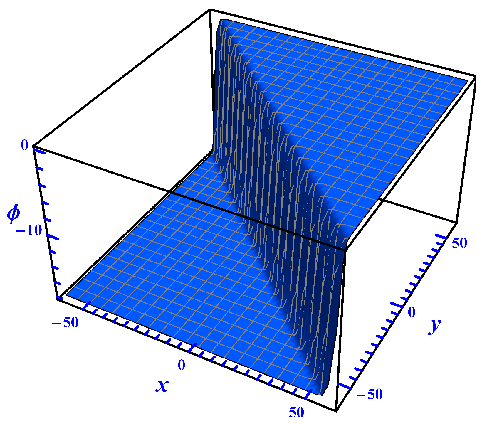
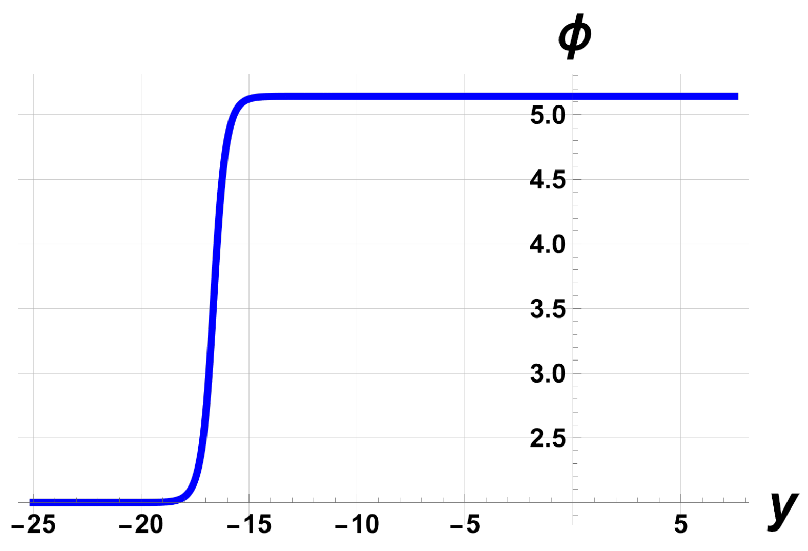
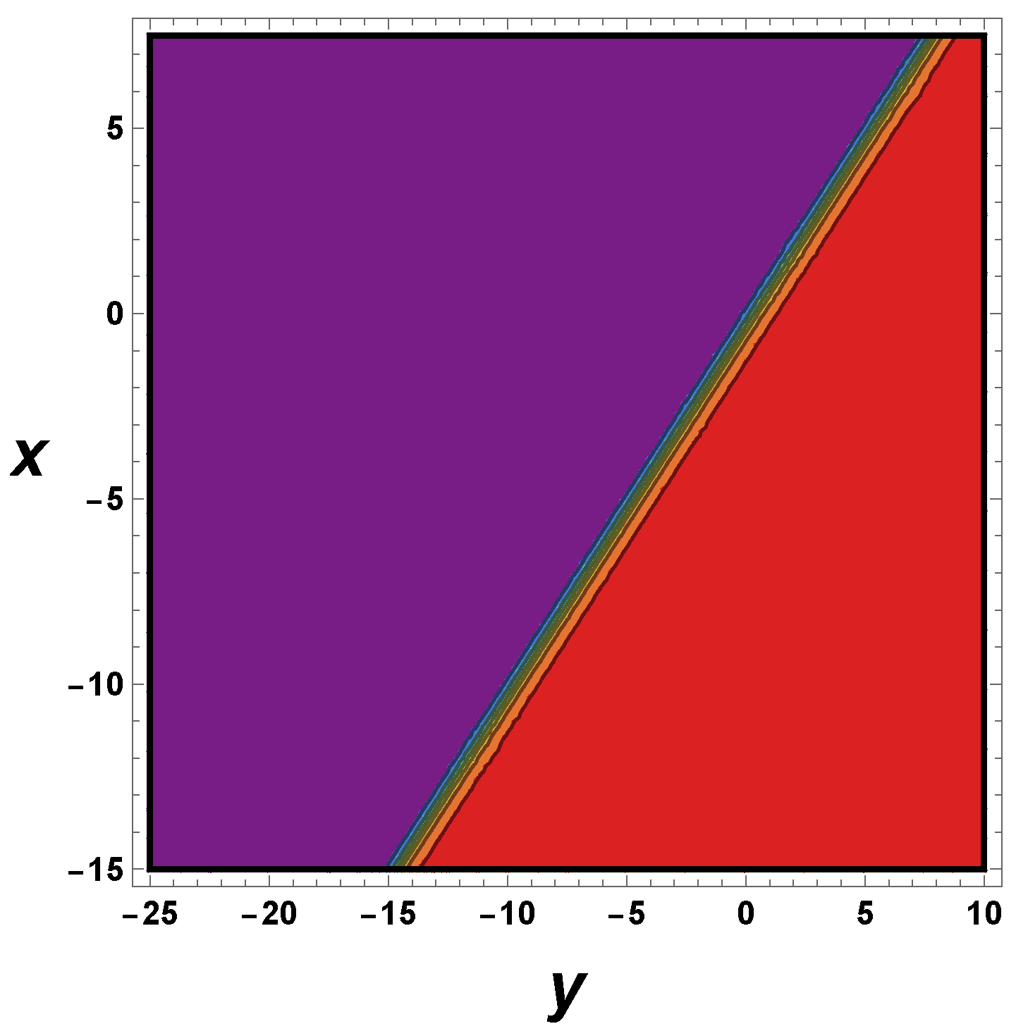
We now apply the Kudryashov method to construct exact solutions of the PKPp Equation (2) for two specific cases, namely, $p=1$ and $p=2$.

4.1. Solutions of (2) with $p=1$ Using the Kudryashov Method

We now find exact solutions of ODE (55) using the Kudryashov method. Let us assume that the solution of Equation (55) is of the form

$$\begin{array}{c}\hfill W\left(z\right)={\displaystyle \sum _{n=0}^N}{\mathcal{A}}_n{\left(Q\left(z\right)\right)}^n,\end{array}$$

(70)

where Q satisfies the first-order nonlinear ODE $Q_z=Q^2-Q.$ Using Step 2 of the method, we obtain $N=1$. So the solution of the ODE (55) is of the form

$$\begin{array}{c}\hfill W\left(z\right)={\mathcal{A}}_0+{\mathcal{A}}_{1}Q\left(z\right).\end{array}$$

(71)

Following the next step, we arrive at the following system of algebraic equations:

$$\begin{array}{ccc}\hfill Q& :& c^2\gamma {\mathcal{A}}_1-2c\gamma \nu {\mathcal{A}}_1+\gamma {\nu }^2{\mathcal{A}}_1-\beta {\mathcal{A}}_1+c{\mathcal{A}}_1=0\hfill \end{array}$$

(72)

$$\begin{array}{ccc}\hfill Q^2& :& 7\beta {\mathcal{A}}_1-c{\mathcal{A}}_1-\gamma {\nu }^2{\mathcal{A}}_1+2\gamma \nu {\mathcal{A}}_1+{\displaystyle \frac{1}{2}}\alpha {\mathcal{A}}_1^2-c^2\gamma {\mathcal{A}}_1=0\hfill \end{array}$$

(73)

$$\begin{array}{ccc}\hfill Q^3& :& \alpha {\mathcal{A}}_1^2+12\beta {\mathcal{A}}_1=0\hfill \end{array}$$

(74)

$$\begin{array}{ccc}\hfill Q^4& :& {\displaystyle \frac{1}{2}}\alpha {\mathcal{A}}_1^2+6\beta {\mathcal{A}}_1=0.\hfill \end{array}$$

(75)

Solving this system of algebraic equations, with the aid of Mathematica, we obtain

$$\begin{array}{c}\hfill {\mathcal{A}}_1={\displaystyle \frac{12}{\alpha }}(2c\gamma \nu -c^2\gamma -\gamma {\nu }^2-c),\beta =c^2\gamma -2c\gamma \nu +\gamma {\nu }^2+c.\end{array}$$

(76)

Therefore, the exact solutions of Equation (55) are given by

$$\Phi \left(z\right)={\mathcal{A}}_0+{\displaystyle \frac{12}{\alpha }}(2c\gamma \nu -c^2\gamma -\gamma {\nu }^2-c)Q\left(z\right),Q\left(z\right)={\displaystyle \frac{1}{1+e^z}}.$$

(77)

Reverting back to the original variables, we obtain the solution of Equation (20) as

$$\varphi (t,x,y)=C+{\displaystyle \frac{12}{\alpha }}(2c\gamma \nu -c^2\gamma -\gamma {\nu }^2-c){(1+e^{x+(c-\nu )y-ct})}^{-1},$$

(78)

where C is an arbitrary constant.

The solution profile of (78) with parameters $C=0,\alpha =2,c=2,\gamma =1,\nu =1,$ and $t=0,$ is given in Figure 1. The solution is showing a sharp gradient indicative of a shock wave or soliton structure. The solution exhibits steep transitions along the $x=y$ direction, with values decreasing significantly across the discontinuity.

4.2. Solutions of (2) with $p=2$ Using Direct Integration

For the case when $p=2$, the resulting ODE, Equation (63), admits a solution through direct integration. The equation is integrated twice and yields the two solutions in the original variables as

$$\varphi (x,y,t)={\displaystyle \frac{2}{\sqrt{\mathcal{A}}}}{tan}^{-1}\left[\sqrt{\mathcal{A}\mathcal{B}}exp\left\{\sqrt{\mathcal{B}}\left(z+C_1\right)\right\}\right]+C_2$$

(79)

and

$$\varphi (x,y,t)={\displaystyle \frac{2}{\sqrt{\mathcal{A}}}}{tan}^{-1}\left[{\displaystyle \frac{1}{\sqrt{\mathcal{A}\mathcal{B}}}}exp\left\{\sqrt{\mathcal{B}}\left(z-C_3\right)\right\}\right]+C_4,$$

where $C_1,C_2,C_3,$ and $C_4$ are arbitrary constants of integration and

$$z=t-cx+(c\nu -1)y,\mathcal{A}={\displaystyle \frac{\alpha }{6\beta }},\mathcal{B}={\displaystyle \frac{c^2\gamma {\nu }^2-2c\gamma \nu +c+\gamma }{\beta c^4}}.$$

The profile structure of the solution (79) is illustrated in the pictures below.

These solution profiles from Figure 2, Figure 3 and Figure 4 are accomplished with $C_1=2$, $C_2=2$, $\beta ={\displaystyle \frac{1}{6}}$, and $\gamma =0.25$, while the other arbitrary parameters are set to one. The spatial variables were restricted to the intervals $-15\le x\le 7.5$ and $-25\le y\le 12.5$. The 3D surface plot in Figure 2 illustrates a solitary wave solution exhibiting a sharp gradient along the $y-$direction, while remaining nearly constant in the $x-$direction. The wavefront transitions smoothly from a lower plateau (purple) to a higher one (red), indicating a kink-type or shock-like structure. This profile reflects the localized nature of the solution in the transverse direction, characteristic of a traveling wave solution governed by nonlinear dispersive dynamics.

It is worth noting that Equation (63) may admit other solutions depending on the specific parameter values. By introducing the substitution $u\left(z\right)=W^{\prime }\left(z\right)$, the equation reduces to a first-order differential equation of the form

$$\begin{array}{c}\hfill {\displaystyle {\left(u^{\prime }\right)}^2=\frac{-1}{\beta c^4}{u}^2\left(\frac{1}{6}\alpha c^4{u}^2+(2c\nu \gamma -c^2{\nu }^2\gamma -c-\gamma )\right).}\end{array}$$

This form reveals the potential for multiple solution branches governed by the sign and structure of the right-hand side. Therefore, under certain parameter regimes, additional exact or implicit solutions may exist. These may be expressed via quadrature, subject to further integration and boundary conditions.

5. Conclusions

By employing Noether’s theorem, we have obtained a number of conservation laws for the potential Kadomtsev–Petviashvili equation with $p-$power nonlinearity (PKPp) along with different values concerning parameter p in this paper. In addition to revealing more of the structure of the PKPp equation, these revealed conservation laws are useful as a basis for finding exact solutions and can be used as tests in numeric simulations, work that is deferred to another investigation. We also obtained new exact solutions for the PKPp equation using the Lie symmetry and Kudryashov methods on their application to cases $p=1,2.$ The Kudryashov method was used because it is a reliable and efficient analytical technique for obtaining exact solutions to nonlinear partial differential equations, especially those involving higher-order derivatives and polynomial nonlinearities. The method is particularly effective in generating rational or solitary wave-type solutions, which are useful for understanding the qualitative behavior of the equation. In the case of Equation (2), applying KM allowed us to construct explicit solutions in a straightforward and systematic manner, making it an appropriate choice for this study. The validity of these solutions has been checked by replacing them into the initial equation using Maple [40]. Our results enrich the characterization of nonlinear equations and can be used in theoretical analysis and numerical simulations as well.

The graphical representation of the wave profile, generated from the Kudryashov method, reveals significant characteristics of the solutions. The 3D plot demonstrates a distinct wave structure with sharp gradients and oscillatory behavior, indicative of soliton-like solutions. This profile highlights the stability and localization of the wave, suggesting that such solutions can model real-world phenomena effectively. The observed peaks represent regions of high amplitude, while the gradual decay at the boundaries illustrates the localized nature of the solutions.

While earlier work by Adem, Khalique, and Biswas [41] focused on finding solutions to the KP equation with power-law nonlinearity in $(1+3)$ dimensions, this study looks at the potential form of the KP equation in $(2+1)$ dimensions, referred to as the PKPp equation. This version of the equation has a different structure and allows for a new type of analysis.

Unlike previous studies that used direct solution methods, this work applies a combination of techniques, including Noether symmetry classification, Lie group analysis, and the Kudryashov method, to find both exact solutions and conservation laws. Another new aspect of this study is the way it classifies the equation’s symmetries depending on the value of the exponent p, which gives more insight into how the equation behaves under different conditions.

In this way, the current study offers a broader and more detailed analysis than what has been done before. It adds to the existing literature by exploring the PKPp equation from a symmetry and conservation point of view.

Overall, the results presented here enhance the mathematical understanding of nonlinear systems with $p-$power nonlinearity and offer new tools for both theoretical and applied research, particularly in the modeling of complex physical systems where such equations arise. Future work could explore further generalizations of the PKPp equation, analyze higher-order symmetries, and investigate their application in real-world scenarios.

References

1. Chatziafratis, A.; Ozawa, T.; Tian, S.F. Rigorous analysis of the unified transform method and long-range instabilities for the inhomogeneous time-dependent Schrödinger equation on the quarter-plane. Math. Ann. 2024, 389, 3535–3602. [Google Scholar] [CrossRef]
2. Wu, Z.; Tian, S. Nonlinear stability of smooth multi-solitons for the Dullin-Gottwald-Holm equation. J. Differ. Equ. 2024, 412, 408–446. [Google Scholar] [CrossRef]
3. Wu, Z.; Tian, S.; Liu, Y.; Wang, Z. Stability of smooth multisolitons for the two-component Camassa–Holm system. J. Lond. Math. Soc. 2025, 111, e70158. [Google Scholar] [CrossRef]
4. Sherawat, A.; Jiwari, R. New multiple analytic solitonary solutions and simulation of (2+1)-dimensional generalized Benjamin-Bona-Mahony-Burgers model. Nonlinear Dyn. 2023, 111, 13297–13325. [Google Scholar]
5. Kumar, V.; Gupta, R.K.; Jiwari, R. Painlevé analysis, Lie symmetries and exact solutions for variable coefficients Benjamin—Bona—Mahony—Burger (BBMB) equation. Commun. Theor. Phys. 2013, 2, 175. [Google Scholar] [CrossRef]
6. Boussinesq, J. Essai sur la théorie des Eaux Courantes; Imprimerie Nationale: Flers en Escrebieux, France, 1877; pp. 1–680. [Google Scholar]
7. Kadomtsev, B.B.; Petviashvili, V.I. On the stability of solitary waves in weakly dispersive media. Sov. Phys. Dokl. 1970, 15, 539–541. [Google Scholar]
8. Xu, P.; Huang, H.; Wang, K. Dynamics of real and complex multi-soliton solutions, novel soliton molecules, asymmetric solitons and diverse wave solutions to the Kadomtsev-Petviashvili equation. Alex. Eng. J. 2025, 125, 537–544. [Google Scholar] [CrossRef]
9. Liu, H.; Shen, J.; Geng, X. Higher-order pole solutions of Kadomtsev-Petviashvili I equation. J. Math. Anal. Appl. 2025, 125, 129718. [Google Scholar] [CrossRef]
10. Asadullah, M.; Javid, A.; Raza, N.; Chahlaoui, Y.; Bekir, A. Envelope solitons and wave structures in the (2+1)-dimensional KP equation. Mod. Phys. Lett. B 2025, 2550174. [Google Scholar] [CrossRef]
11. Qawaqneh, H.; Alrashedi, Y.; Ahmad, H. Discovery of exact solitons to the fractional KP-MEW equation with stability analysis. Eur. Phys. J. Plus 2025, 140, 316. [Google Scholar] [CrossRef]
12. Bhan, C.; Karwasra, R.; Malik, S.; Kumar, S.; Arnous, A.H.; Sha, N.A.; Chung, J. Bifurcation, chaotic behavior and soliton solutions to the KP-BBM equation through new Kudryashov and generalized Arnous methods. AIMS Math. 2024, 9, 8749–8767. [Google Scholar] [CrossRef]
13. Humbu, I.; Muatjetjeja, B.; Motsumi, T.G.; Adem, A.R. Multiple solitons, periodic solutions and other exact solutions of a generalized extended (2+1)-dimensional Kadomstev–Petviashvili equation. J. Appl. Anal. 2024, 30, 197–208. [Google Scholar] [CrossRef]
14. Senthilvelan, M. On the extended applications of homogenous balance method. Appl. Math. Comput. 2001, 123, 381–388. [Google Scholar] [CrossRef]
15. Kaya, D.; El-Sayed, S.M. Numerical soliton-like solutions of the potential Kadomtsev-Petviashvili equation by the decomposition method. Phys. Lett. A 2003, 320, 192–199. [Google Scholar] [CrossRef]
16. Li, D.; Zhang, H. Symbolic computation and various exact solutions of potential Kadomtsev-Petviashvili equation. Appl. Math. Comput. 2003, 145, 351–359. [Google Scholar]
17. Xian, D.; Dai, Z. Application of Exp-function method to potential Kadomtsev-Petviashvili equation. Chaos Soliton Fract. 2009, 42, 2653–2659. [Google Scholar]
18. Inan, I.E.; Kaya, D. Some exact solutions to the potential Kadomtsev-Petviashvili equation and to a system of shallow water wave equations. Phys. Lett. A 2006, 355, 314–318. [Google Scholar] [CrossRef]
19. Ablowitz, M.J.; Segur, H. Solitons and the Inverse Scattering Transform; SIAM: Philadelphia, PA, USA, 1981. [Google Scholar]
20. Wang, M.; Chen, X. Exact solutions for nonlinear evolution equations modified by power-law terms. Appl. Math. Comput. 2015, 269, 632–641. [Google Scholar]
21. Bluman, G.W.; Kumei, S. Symmetries and Differential Equations; Springer: Berlin/Heidelberg, Germany, 1989. [Google Scholar]
22. Ibragimov, N.H. A new conservation theorems. Appl. Math. Comput. 2007, 333, 311–328. [Google Scholar] [CrossRef]
23. Anco, S.C.; Bluman, G.W. Direct construction method for conservation laws of partial differential equations. Part I: Examples of conservation law classifications. Eur. J. Appl. Math. 1997, 13, 545–566. [Google Scholar] [CrossRef]
24. Xian, D.; Chen, H. Symmetry reductions and new exact non-traveling wave solutions of potential Kadomtsev–Petviashvili equation with p-power. Appl. Math. Comput. 2010, 216, 70–79. [Google Scholar] [CrossRef]
25. Gupta, R.K.; Bansal, A. Painleve analysis, Lie symmetries and invariant solutions of potential Kadomtsev-Petviashvili equation with time dependent coefficients. Appl. Math. Comput. 2013, 219, 5290–5302. [Google Scholar]
26. Xian, D.; Chen, H. Symmetry reduced and new exact non-traveling wave solutions of potential Kadomtsev-Petviashvili equation with p-power. Appl. Math. Comput. 2010, 217, 1340–1349. [Google Scholar] [CrossRef]
27. Sebogodi, M.C.; Muatjetjeja, B.; Adem, A.R. Exact solutions and conservation laws of a (2+1)-dimensional combined potential kadomtsev-petviashvili-b-type kadomtsev-petviashvili equation. Int. J. Theor. Phys. 2023, 62, 165. [Google Scholar] [CrossRef]
28. Afolabi, O.A.; Johnpillai, A.G. Exact solutions of generalized KP equations using Kudryashov and Lie symmetry methods. Results Phys. 2021, 25, 104311. [Google Scholar]
29. Alquran, M.; Mohd, N.A. Wave structures and solutions of KP-type equations via analytical techniques. J. Math. 2022, 12, 2042. [Google Scholar]
30. Umaru, M.A.; Mahgoub, A. Noether symmetries and conservation laws of nonlinear evolution equations in 2D. Symmetry 2023, 15, 870. [Google Scholar]
31. Muatjetjeja, B.; Khalique, C.M. Symmetry analysis and conservation laws for a coupled (2+1)-dimensional hyperbolic system. Commun. Nonlinear Sci. Numer. Simulat. 2015, 22, 1252–1262. [Google Scholar] [CrossRef]
32. Noether, E. Invariante variationsprobleme. Math. Phys. Kl. Heft 1918, 2, 235–257. [Google Scholar]
33. Olver, P.J. Applications of Lie Groups to Differential Equations, Graduate Texts in Mathematics, 2nd ed.; Springer: Berlin, Germany, 1993. [Google Scholar]
34. Kudryashov, N.A. One method for finding exact solutions of nonlinear differential equations. Commun. Nonlinear Sci. Numer. Simulat. 2012, 17, 2248–2253. [Google Scholar] [CrossRef]
35. Kudryashov, N.A. Solitons of the complex modified Korteweg–de Vries hierarchy. Chaos Solitons Fractals 2024, 184, 115010. [Google Scholar] [CrossRef]
36. Ege, S.M.; Misirli, E. The modified Kudryashov method for solving some fractional-order nonlinear equations. Adv. Differ. Equ. 2014, 135, 1–13. [Google Scholar] [CrossRef]
37. Hubert, M.B.; Betchewe, G.; Doka, S.Y.; Crepin, K.T. Soliton wave solutions for the nonlinear transmission line using the Kudryashov method and the (G/G)-expansion method. Appl. Math. Comput. 2014, 239, 299–309. [Google Scholar] [CrossRef]
38. Zayed, E.M.E.; Moatimid, G.M.; Al-Nowehy, A. The generalized Kudryashov method and its applications for solving nonlinear PDEs in mathematical physics. Sci. J. Math. Res. 2015, 5, 19–39. [Google Scholar]
39. Islam, M.S.; Khan, K.; Arnous, A.H. Generalized Kudryashov method for solving some (3+1)-dimensional nonlinear evolution equations. New Trends Math. Sci. 2015, 3, 46–57. [Google Scholar]
40. Cheviakov, A.F. GeM software package for computation of symmetries and conservation laws of differential equations. Comput. Phys. Commun. 2007, 176, 48–61. [Google Scholar] [CrossRef]
41. Adem, A.R.; Khalique, C.M.; Biswas, A. Solutions of Kadomtsev–Petviashvili equation with power law nonlinearity in 1+3 dimensions. Math. Method Appl. Sci. 2011, 34, 532–543. [Google Scholar] [CrossRef]
Figure 1. Exact solution of the PKPp equation plotted in 3D, showing a sharp gradient indicative of a shock wave or soliton structure.
Symmetry 17 01053 g001
Figure 2. Three-dimensional simulation of solution (79).
Symmetry 17 01053 g002
Figure 3. Two-dimensional simulation of solution (79).
Symmetry 17 01053 g003
Figure 4. Heat map simulation of solution (79).
Symmetry 17 01053 g004
Disclaimer/Publisher’s Note: The statements, opinions and data contained in all publications are solely those of the individual author(s) and contributor(s) and not of MDPI and/or the editor(s). MDPI and/or the editor(s) disclaim responsibility for any injury to people or property resulting from any ideas, methods, instructions or products referred to in the content.