Few-Grid-Point Simulations of Big Bang Singularity in Quantum Cosmology

Abstract

In the context of the current lack of compatibility of the classical and quantum approaches to gravity, exactly solvable elementary pseudo-Hermitian quantum models are analyzed, supporting the acceptability of a point-like form of the Big Bang. The purpose is served by a hypothetical (non-covariant) identification of the “time of the Big Bang” with Kato’s exceptional-point parameter $t=0$. The consequences (including the ambiguity of the patterns of unfolding the singularity after the Big Bang) are studied in detail. In particular, singular values of the observables are shown to be useful in the analysis.

1. Introduction

The determination of the age of our Universe (i.e., an estimated $13.787\pm 0.02$ billion years) is, undoubtedly, one the most impressive achievements of experimental astronomy [1,2]. In parallel, the hypothetical birth of the Universe at zero diameter and zero time $t=0$ (called the Big Bang singularity, cf. its schematic picture in Figure 1) finds a consistent explanation and interpretation in Einstein’s formalism of general relativity.

In the latter framework, the question of “what happened before the Big Bang?” is usually considered irrelevant. Incidentally, a different opinion has been formulated by Penrose, who conjectured that the Universe might have existed even before the Big Bang [3]. Its prehistory is to be perceived as eternal, composed of a series of Aeons, well separated by their collapses (or, more precisely, by the stages of an unlimited expansion tractable also as an “entropic death”), followed by a re-birth and subsequent expansion (notice that the term “Big Bang” itself was originally coined as a mockery (!)).

A comment on Penrose’s eternal cyclic cosmology hypothesis was given in our recent paper [4]. We pointed out that before the Big Bang, the two alternative scenarios, as displayed in Figure 1 and Figure 2, are just extremes. Besides these two options (i.e., besides the assumption of no or of an unchanged observable space at $t<0$, respectively), it would be possible to consider a certain “evolutionary” cosmology in which the structure of the older Aeon can be, vaguely speaking, “underdeveloped”.

In the language of our schematic pictures, Figure 3 can be seen as an illustration in which one registers just two “observable” grid points at $t<0$. A more explicit illustration of such an evolutionary scenario can be found in our older paper [5], where we considered ten observable points at $t>0$. In our subsequent paper, [6] the schematic “four-point” old Aeon was studied as evolving into an“eight-point” (i.e., strictly twice as large) new Aeon.

In all of the latter papers, it had to be emphasized that the transition from classical Big Bang scenarios to their quantum mechanical descendants involves a number of significant conceptual leaps. The reason for this is that at present, we do not have a fully consistent quantum version of Einstein’s classical theory at our disposal. Still, even on the present level of our understanding of quantized theory, a prevailing opinion is that after quantization, the Big Bang singularity of classical theory must necessarily be replaced by a regularized mechanism in a process called the “Big Bounce” (cf., e.g., [7] or section 8 in [8]). In Rovelli’s words, the quantization-related “absence of singularities” is in fact “what one would expect from a quantum theory of gravity”(see p. 297 in loc. cit.).

Temporarily dominant as it was, this opinion has recently been challenged by Wang and Stankiewicz [9], who claimed that in their theory, “the quantized Big Bang is not replaced by a Big Bounce”. This was precisely the reason why we formulated our present project and, in particular, why we decided to study the problem of the possible survival of singularities after quantization via elementary models.

The presentation of our results will be preceded by Section 2, in which we will introduce the basic concepts and, first of all, the interpretation of the Big Bang as a phenomenon characterized by the time dependence of the geometry of the conventional 3D space. For our present methodical purposes, the time dependence of this geometry will be simulated, in a manifestly non-covariant manner, by the time dependence of a few representative spatial grid points $x_n\left(t\right)$.

In Section 3, we will accept the hypothesis that the “initial” Big Bang singularity will not be “smeared out” by the quantization and that its survival can find a consistent mathematical ground in Kato’s [10] concept of exceptional points (EPs).

A more explicit search for consequences of these assumptions will be started in Section 4, in which the underlying Hilbert space of quantum states will be assumed to be two-dimensional, and in which the quantum grid-point operator $X\left(t\right)$ representing (or rather sampling) the geometry will be just a two-by-two complex and symmetric matrix. A key message of our present paper (viz., a recommendation that one should pay attention to the singular values rather than to the eigenvalues of $X\left(t\right)$) finds its first and most elementary and transparent illustration here.

A series of a few less elementary N by N toy models will be then analyzed in Section 5 (in which our illustrative matrices $X\left(t\right)$ remain to be complex and symmetric) and Section 6 (where a different class of toy models is studied in order to demonstrate a certain model-independence of our observations and conclusions).

Our observations will be thoroughly discussed in Section 7, where we will briefly review some of the basic challenges encountered during the attempted quantization of the Big Bang on a more general and example-independent level. Finally, our results will be briefly summarized in Section 8.

2. 3D Space and Its Few-Grid-Point Representations

Our present study was motivated by the toy models as sampled by Figure 3, in which one expects that after quantization, the time-dependent positions $x_n\left(t\right)$ of the grid points should be treated as eigenvalues of a suitable “grid-point” operator $X\left(t\right)$. In Figure 3 itself, only two eigenvalues remain real before the Big Bang. The other two eigenvalues are not displayed because they are not observable. The corresponding quantum states (spanning an unphysical part of the Hilbert space) have to be treated and decoupled as “ghosts” [5].

In the current physics-oriented literature, the treatment of the problem of ghosts (i.e., of the candidates $X\left(t\right)$ for the operators of observables with the mixed real or real plus complex spectra) is still inconclusive (cf. [6,11]). Paradoxically, therefore, our present project of study of the schematic models of the Big Bang singularity in quantum cosmology will be mainly guided by the recent progress achieved by mathematicians.

In this direction, in particular, Pushnitski with Štampach [12] suggested a new direction of research by proposing a turn of attention from the information about the system mediated by the mixture of the real and complex eigenvalues (this information is complete but complicated) to its reduced form, represented by the real quantities called singular values.

We will follow the guidance.

2.1. Grid Points in Conventional Hermitian Quantum Theory

Without any reference to Penrose’s cyclic–cosmology realization of the crossover between Aeons (mediated by a conformal scaling and, hence, not quite characterized by our present Figure 2), the related transition is, formally, the simplest possible scenario in the classical physics framework. The collapse and expansion transmutation of the 3D space can be then sampled by a multiplet of some arbitrary representative time-dependent grid points (i.e., after the present simplification, by a 1D quadruplet $x_n\left(t\right)\in \mathbb{R}$).

On the classical physics level, even Penrose himself had and has multiple opponents. Some of them claimed that we cannot consistently speak about the time before the Big Bang so that, in our present graphical language, Figure 2 and Figure 3 have to be rejected as over-speculative. Another and, by far, the more relevant counter-argument by the opponents reflected the fact that due to the high-density and high-temperature nature of the initial stage of evolution of our present Universe, the description of the Big Bang must necessarily be quantum–theoretical.

The recent progress in the quantization of gravity (cf., first of all, its loop quantum gravity form [8,13,14]) could be recalled as strong (though not ultimate [9]) support of the above-mentioned intuitive expectation that the point-like classical Big Bang singularity has to be smeared out, yielding, after quantization, something like the Big Bounce [7]. In graphical language, such a disappearance of singularity can be illustrated by Figure 4, which samples how the Big Bang-related crossing of eigenvalues happens to become “avoided”.

2.2. Grid Points in Pseudo-Hermitian Quantum Theory

The innocent-looking assumption of Hermiticity $X\left(t\right)=X^{†}\left(t\right)$, as accepted in Figure 4, is of a predictive theoretical relevance. The point is that the removal of this assumption would reopen the possibility of the existence of a mathematically fully consistent point-like form of the Big Bang singularity.

In the abstract framework of quantum theory, one of the most straightforward realizations of a return to the singularity-admitting evolutions is offered by the so-called pseudo-Hermitian theory [15,16,17]. In such a theory, the operators representing observables can be non-self-adjoint. One can build a simplified, non-covariant model of the evolution of the Universe in which the space-sampling grid-point operator is non-Hermitian:

$$X\left(t\right)\ne X^{†}\left(t\right).$$

This is the key assumption that enables one to achieve the simultaneous degeneracy of all (or at least of some) of the eigenvalues of $X\left(t\right)$ at the Big Bang time $t=0$ in a way compatible with the classical point-like Big Bang hypothesis:

$$\underset{t\to 0}{lim}{x}_n\left(t\right)=x\left(0\right),n=1,2,\dots ,N.$$

(1)

In mathematics, Kato [10] proposed that such a parameter (i.e., $t=0$ in our time scale) be called an “exceptional point” (EP). In physics, Heiss [18,19] calls its use “ubiquitous”. In [20], in particular, we explained that in the quantum theory of gravity, the tentative point-like EP interpretation of the Big Bang might prove tenable.

3. Quantum Big Bang as Exceptional Point

A number of the related conceptual as well as technical open problems is enormous [8]. In our present paper, we felt inspired, in particular, by the fact that after one postulates the existence of the same toy-model grid-point operator $X\left(t\right)$ before and after the Big Bang, one immediately has to distinguish between the two alternative before-the-Big-Bang evolution scenarios, as characterized by our two schematic Figure 1 and Figure 2.

From a more abstract mathematical perspective, the different choices of $X\left(t\right)$ need not necessarily stay restricted just to one of the latter two options. Indeed, besides Figure 1 (in which the $t<0$ spectrum is all unobservable, complex) and besides Figure 2 (in which the whole $t<0$ spectrum is assumed to be real), one can easily imagine the existence of many other $t<0$ spectra that may only be partially real (cf. Figure 3).

We have hardly any opportunity to test the hypotheses concerning the properties of the Universe during the pre-Big-Bang “Aeon” (but no certainty—see [21]). One could even feel skeptical concerning the reliability of any experiment-based insight into the structure of the 3D space shortly after the current Big Bang. Thus, one cannot exclude a survival of some complex (i.e., unobservable) eigenvalues of $X\left(t\right)$ at any time $t<0$ or $t>0$.

The requirement of an extension of the class of the hypothetical cosmological quantum models beyond the two extreme simplifications sampled by Figure 1 and Figure 2 is also motivated by a broader mathematical experience and physical context: Pars pro toto, let us recall paper [22], which suggested a typical many-body model in which the authors worked with non-Hermitian operators.

3.1. Alternative Unfolding Patterns

Before we proceed to the formulation of our project, let us note that what remains unclear is the very applicability of a consistent quantization of such a generalized approach to the Big Bang problem.

In this setting and, in particular, in the cosmological Big Bang context, the use of exactly solvable models can be found to be indispensable. Although the detailed analysis of such models need not necessarily lead to phenomenological and experimentally verifiable predictions, it can certainly complement at least some of the existing cosmological speculations about issues like an observability of the traces of what happened before the Big Bang [3,21], or like the question of the existence or absence of a Big Bang singularity in cosmology after quantization [7,9,23].

During the purely mathematical study of dynamics of a toy-model quantum Universe near its hypothetical EP-related singularity (located at $t=0$ in our figures), we might wish not to distinguish between the $t>0$ evolution after the Big Bang and the $t<0$ evolution before the Big Bang. Nevertheless, a necessary return from mathematics to physics would immediately force us to see a deep contrast between our ability to design experiments in the current or in the preceding Aeon.

Although the strength of this contrast has partially been denied by Penrose et al. [3], the natural asymmetry between the pre-Bang and post-Bang era (i.e., in Penrose’s terminology, Aeon), it might make sense to keep it implicitly in mind even during our forthcoming methodical coverage of both of these regimes on a more or less equal footing.

Even under such an idealization of possible physics behind our present toy models of the Big Bang (admitting the loss of the reality of the spectrum at both signs of the time t), we are not going to classify and study the general cases, having in mind that our present methodical purposes will be well served even when we choose, for our explicit illustrative calculations, just the models in which the spectrum would have most general structure of Figure 3.

A decisive methodical advantage of the latter choice is that the models will support both the real and complex eigenvalues. Still, our present observations will be far from conclusive. Long before their possible completion in the future, our methodically motivated simulations of the quantum Big Bang event may help even though they were only made feasible after their truly drastic simplifications.

3.2. Vicinity of Quantum Big Bang

In our recent study [24], we pointed out that one of the eligible consistent descriptions of a point-like quantum Big Bang (i.e., of a strictly quantum analogue of Figure 1 or Figure 2) could be provided via the pseudo-Hermitian reformulation of conventional quantum theory (see, e.g., review [15]). Such a description has to be based on an identification of the Big Bang instant $t=0$ with Kato’s exceptional point parameter (EP, [10]). In the manner supported by an illustrative example, we demonstrated that such an identification could be feasible. Now, we plan to support the claim through a deeper technical analysis.

From a broader conceptual point of view, the main weakness of the EP-based picture of the birth of the Universe is that the support of its validity remained restricted to the specific subclass of exceptional points, namely, to those evolution patterns which can be characterized, in our intuitive graphical presentation, by Figure 1 or Figure 2. This strictly requires that after the Big Bang event (i.e., at $t>0$), all of the eigenvalues $x_n\left(t\right)$ of an admissible physical grid-point operator $X\left(t\right)$ remain real. Simultaneously, all or none of them have to be real at $t<0$, i.e., before the Big Bang event.

Even in the context of pure mathematics, both of the respective latter postulates (viz., of Penrose’s “cyclic re-birth”, or of a more pragmatic hypothesis of “nothing before the Big Bang”) must be considered over-restrictive. A reduction of the picture to these two extremes can hardly be considered satisfactory also from a purely phenomenological perspective. Indeed, we may recall, for comparison, the situation in many-body physics. In the framework of the Bose–Hubbard model, the study of exceptional points by Graefe et al. [22] revealed that although an extreme scenario, as sampled here by Figure 1, does exist, its occurrence only represents a very small fraction of all of the mathematically admissible alternatives. The latter authors observed that in spite of the fairly realistic background of their model, the emergence of a complex part in any eigenvalue can hardly be excluded. In the vicinity of a generic EP, in general, some of the eigenvalues happened to remain real (i.e., observable) and some of them not.

The same mixed spectra can be expected to occur also in the EP-based cosmological applications. This is more so near the quantum Big Bang, where the grid-point operators $X\left(t\right)$ are introduced, in most cases, via a purely pragmatic and physics-oriented process. Hence, the complexity of at least some of the eigenvalues should be perceived as generic.

In the vicinity of the EP parameter $t=0$, as a consequence, the quantum system in question (i.e., in our case, the quantum Universe) will have to be treated by the methods that are usually used for the description of the open systems with resonances [25]. Having this in mind, we will study the general EP-unfolding process via several elementary but non-numerically tractable toy models.

3.3. Unobservable Grid Points

In paper [22], the model has been kept simple while still admitting the non-real elements in the spectrum. In the most conventional context of quantum mechanics of many-body systems, the authors worked with a parameter-dependent non-Hermitian Hamiltonian, yielding both the bound and resonant states. They were able to study and describe the parameter dependence of the spectra using standard mathematical techniques including not only numerical but also analytic and perturbative ones.

The feasibility of these techniques will decrease with an increase in the complexity of the operator. Once we plan to turn attention to quantum cosmology and the Big Bang, the acceptance of some truly drastic simplifications seems necessary.

Even though we decided to mimic just the passage of the Universe through its spatial singularity using a grid-point toy-model operator $X\left(t\right)$, we will have to treat time as a parameter. What we gain is that the dynamics of any underlying “spatial background” becomes quantized. What we lose are the chances of having our picture of reality covariant.

Although we insist on the reality of $x\left(0\right)$ in Equation (1), we will assume just a partial observability of the Universe near the Big Bang. This will enable us to obtain a certain source of the observational signatures which could distinguish our present, EP-based quantum Big Bang scenario from its various conventional alternatives. Thus, in a small but, in principle, both-sided vicinity of $t=0$, we will admit the complexity of at least some of the eigenvalues of $X\left(t\right)$:

$$\exists n,t\mathrm{that}{x}_n\left(t\right)\in \mathbb{C}.$$

For virtually any sufficiently realistic and general choice of $X\left(t\right)$, the latter assumption would make the evaluation of its spectrum complicated. This is the very core of the problems, which will be addressed in what follows.

4. Two-Grid-Point Simulation of Big Bang

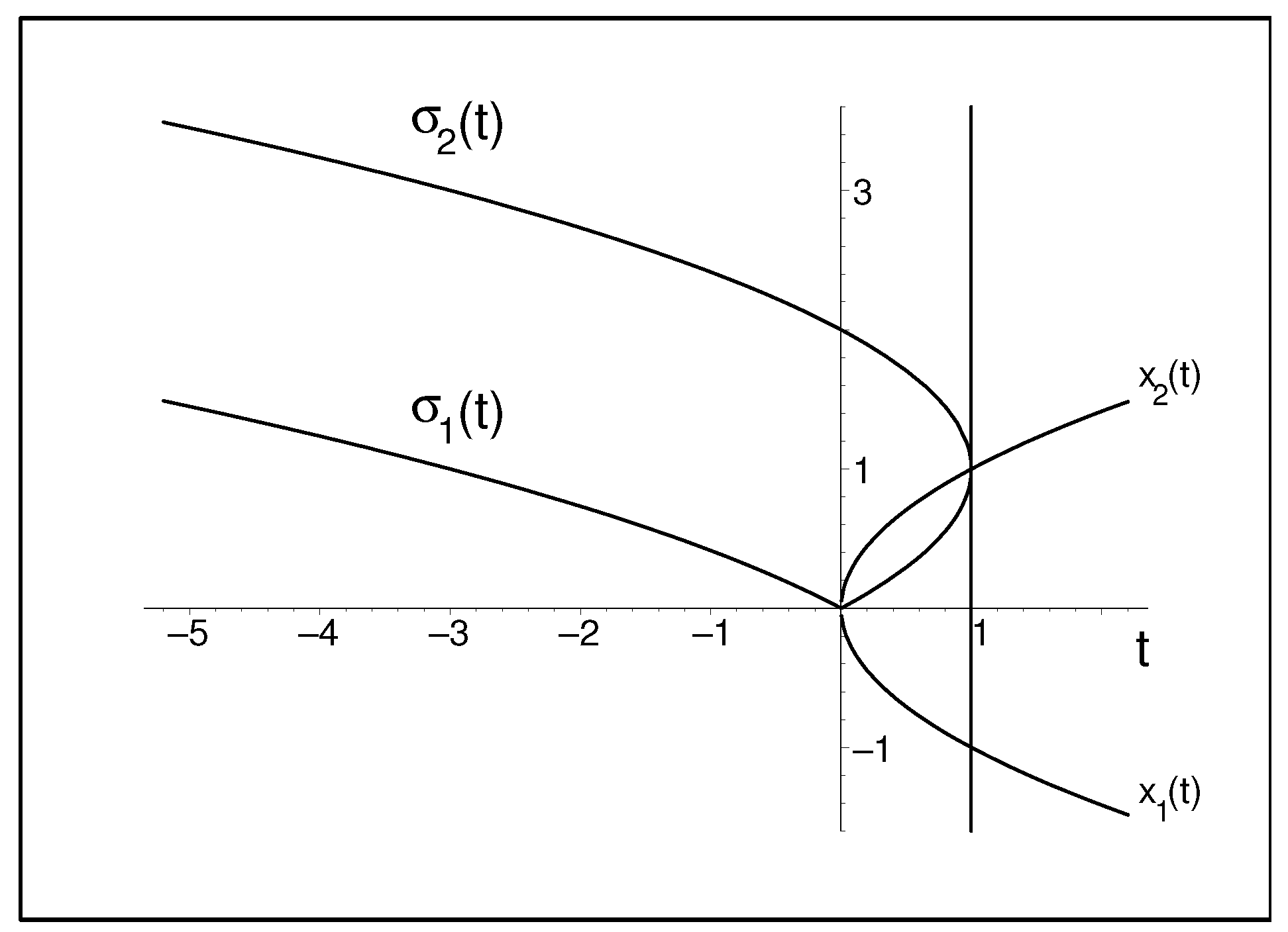
A part of the reason why we intend to reduce the study of the eigenvalues $x_n\in \mathbb{C}$ to the study of singular values ${\sigma }_n\in \mathbb{R}$ can be seen in the rather serious technical obstacles encountered during the numerical localization of complex eigenvalues. The most immediate insight into some properties of this reduction can be provided when we replace the operators with matrices. For a deeper understanding of the correspondence between the physics of the evolution of the Universe near the Big Bang and the mathematics of the unfolding of the EP-based degeneracies of the quantum grid-point spectra, it makes sense to mimic these processes using a few most elementary toy models.

4.1. Grid-Point Operator $X\left(t\right)$: Complex Symmetric Choice

A particularly transparent explicit illustration of the mechanism of the EP-based unavoided crossings of the time-dependent eigenvalues $x_n\left(t\right)$ of the time-dependent and manifestly non-Hermitian operators $X\left(t\right)$ is offered by the following two-by-two-matrix grid-point-operator toy model:

$$X\left(t\right)=\left[\begin{array}{cc}-it& 1\\ 1& it\end{array}\right]$$

(2)

which is easily diagonalized, as follows:

$$X\left(t\right)\to \left(t\right)=\left[\begin{array}{cc}\sqrt{1-t^2}& 0\\ 0& -\sqrt{1-t^2}\end{array}\right].$$

The two-level spectrum of such a model is strictly real if and only if $t\in [-1,1]$ (see the circle in Figure 5). This is a closed interval but its endpoints are Kato’s exceptional points. They are manifestly unphysical because matrix (2) ceases to be diagonalizable in the limit of $t\to \pm 1$.

Such an observation enables us to treat the matrix of Equation (2) as a highly schematic model of the two-grid-point Universe in two ways. In its first, “Big Bang” interpretation (which would be conceptually analogous to Figure 1 above) we may localize the Big Bang event at $t_{\left(BB\right)}^{EP)}=-1$, and we will have to keep our “age of the Universe” well below the origin in suitable units, $-1<t\ll 0$.

In another complementary “Big Collapse” interpretation of the model, we could localize another “inverse” Big Collapse event at $t_{\left(BC\right)}^{EP)}=+1$ while keeping the time of the “end of life of the preceding Aeon” well separated from the origin, with, perhaps, $0\ll t<1$ in some other suitable units.

Along the rest of the real line of time (and, in both Aeons, sufficiently far from the origin, i.e., for $\left|t\right|>1$), the grid-point spectrum of the model becomes purely imaginary: see the hyperbolic curve graph of $|\mathrm{Im}{x}_n\left(t\right)|$ in Figure 6. This would make the 3D space, naturally, hardly observable, in the conventional current perception of the theory at least.

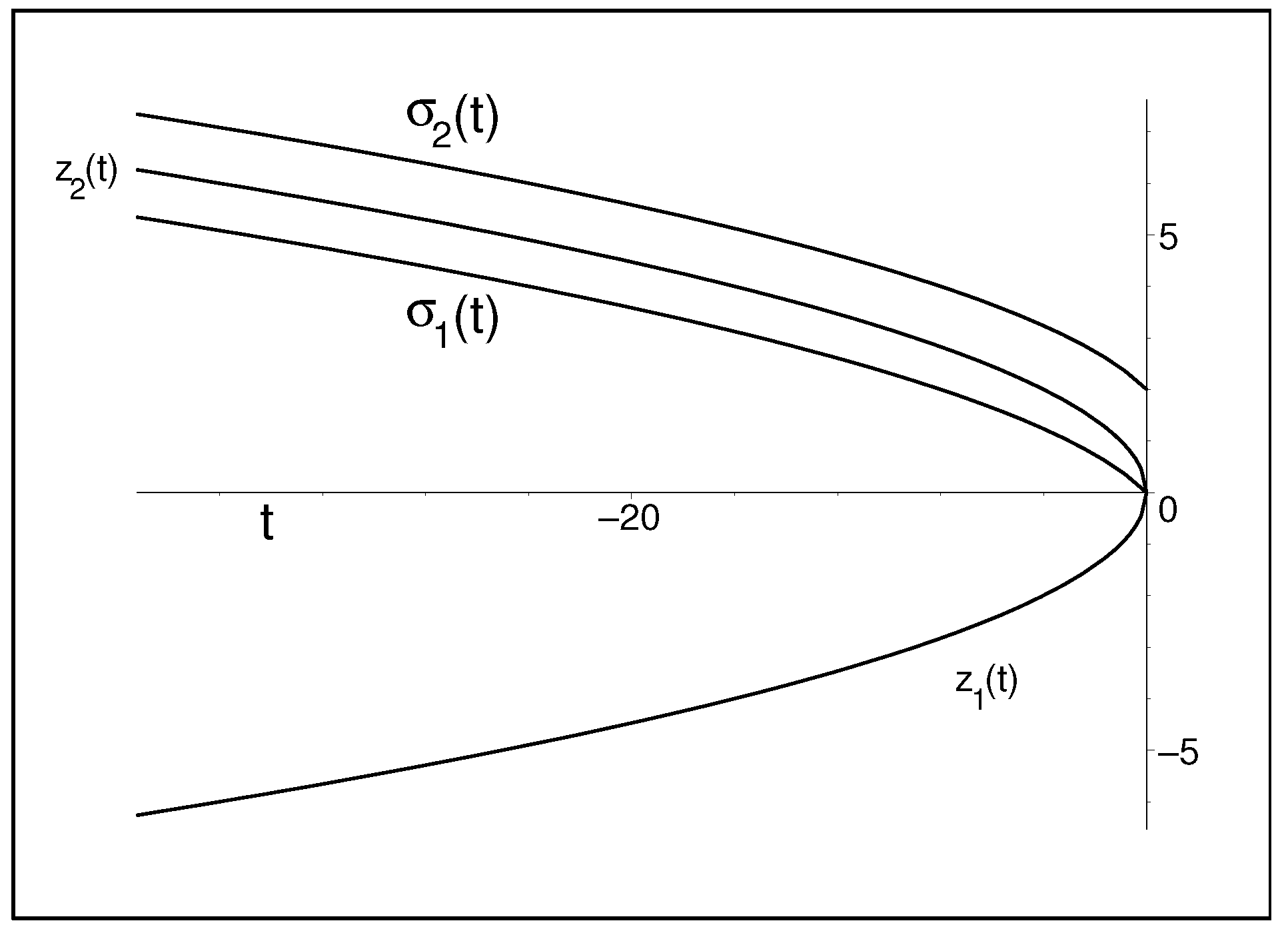
4.2. The Role of Singular Values

In contrast to the curves representing the spectra, the singular values ${\sigma }_n\left(t\right)$ are, in our pictures, real, linear, and non-negative functions of time at all $t\in (-\infty ,\infty )$. Once we restrict attention to the upper halves of the spectral curves, a quick inspection of our two pictures reveals that every such curve lies inside a strip defined by singular values. In other words, it is minimized and maximized (we may say “bracketed”) by the two singular-value lines.

In particular, inside the “observable Aeon” interval of $t\in (-1,1)$, Figure 5 indicates that the bracketing applies to the real and positive eigenvalue (plus, after the mere change of sign, also to the other, negative eigenvalue). For $t\notin (-1,1)$ (i.e., far from the origin), the other Figure 6 shows how the same bracketing applies to the absolute value of the complex eigenvalue. The (in principle, simpler) evaluation of singular values appears useful, for the purposes of a rough spectral estimate at least.

Various forms of the bracketing properties of the (always real) singular values is well known in mathematics. In the context of physics, one should only keep in mind that strictly speaking, our most elementary toy-model operator $X\left(t\right)$ of Equation (2) loses its status of an observable at $t\notin (-1,1)$. Still, there exist phenomenological reasons due to which even the complex eigenvalues $x_n\left(t\right)$ have to be evaluated and reinterpreted, say, as characteristics of an unstable quantum system.

The closest analogy of such a situation can be found in the emergence of unstable resonances in the so-called open quantum systems, say, in nuclear, atomic, or molecular physics [25]. A return to stability as encountered at $t\in (-1,1)$ can be then perceived as a physics-specifying emergence of an observable spatial position in our toy model. A return to the reality of the eigenvalue implies a return to the observability of grid points. Once we have to predict an outcome of a measurement, we have to localize them as precisely as possible. For this reason, the bracketing may play the role of a rough estimate.

The complexity of the eigenvalues is often interpreted as a more or less unavoidable consequence of an influence of an (in principle, unknown) “environment”. Still, even if one accepts such a philosophy as “more realistic”, another obstacle emerges from the necessary generalization of the underlying mathematics. Whenever the eigenvalues happen to be complex, their practical numerical evaluation becomes technically much more complicated.

This is the reason why, in practice, the localization of complex eigenvalues is often being replaced by the evaluation of singular values. The process is simpler because the singular values remain real. Last but not least, their definition is comparatively easy. For any non-Hermitian matrix Q, it coincides with the non-negative square roots of eigenvalues of an associated, manifestly Hermitian matrix product $Q^{†}Q$.

It is worth adding that our toy-model matrix (2) can be interpreted as parity–time-symmetric alias $\mathcal{PT}$-symmetric [26,27] alias Krein-space Hermitian [28,29]. Due to such an additional symmetry, the form (i.e., the time dependence) of its singular values ${\sigma }_n\left(t\right)$ is simpler than that of the eigenvalues $x_n\left(t\right)$ themselves.

In order to see this, we only have to recall the definition by which the singular value of $X\left(t\right)$ is just a (plus-sign) square root of an eigenvalue of the product

$$\mathbb{X}\left(t\right)=X^{*}\left(t\right)X\left(t\right)=\left[\begin{array}{cc}{t}^2+1& 2it\\ -2it& t^2+1\end{array}\right].$$

The diagonal isospectral partner of the latter matrix is easily evaluated:

$$\tilde{\mathbb{X}}\left(t\right)=\left[\begin{array}{cc}{t}^2+1+2t& 0\\ 0& t^2+1-2t\end{array}\right].$$

Although the spectrum of $X\left(t\right)$ becomes complex at $\left|t\right|>1$, the singular values of the same operator both remain real along the whole real axis of t.

For illustration, a comparison of the two alternative characteristics of model (2) is displayed in Figure 6. One discovers there a nontrivial relationship between the eigenvalues and singular values in the unstable-state dynamical regime. The picture demonstrates that the knowledge of the singular values ${\sigma }_n\left(s\right)$ offers, in fact, truly nontrivial information about the spectrum of the matrix even when this spectrum is complex.

Another serendipitous benefit of the model is that the elementary time dependence of our grid-point matrix $X\left(t\right)$ of Equation (2) appears to be reflected by the equally elementary (viz., linear) time dependence of its singular values ${\sigma }_n\left(t\right)$. Therefore, in Figure 5 and Figure 6, the singular values appear as straight lines.

The climax of the story can be seen in the fact that, in contrast to the user-friendly scenario with the real spectrum at $t\in (-1,1)$, the phenomenon of bracketing continues to play a useful role at $t\notin (-1,1)$. According to Figure 6, the bounds imposed upon the imaginary parts of the eigenvalues, as provided by the singular values, look, for practical purposes, impressive.

Although the spectrum-bracketing property, as sampled by Figure 6, may look like an artifact emerging in a specific model, one should recall the existing mathematics behind the singular values in order to find a general theory of the related inequalities.

The only remaining question is whether such an observation of bracketing is not too model-dependent. Independent tests are necessary.

5. More Grid Points

For the majority of the larger N by N matrices, the search for the eigenvalues and singular values is a purely numerical task, in general. Still, there are exceptions. For illustration, let us first recall the N by N matrices of paper [30].

Nothing truly new emerges when one moves from the above-considered matrices of dimension $N=2$ to the models with larger N (for the sake of definiteness, we may and will keep these dimensions even). We will see that the evaluation of the singular values and, in particular, their bracketing property, can still offer fairly nontrivial insight into the structure and dynamics of the quantum system in question.

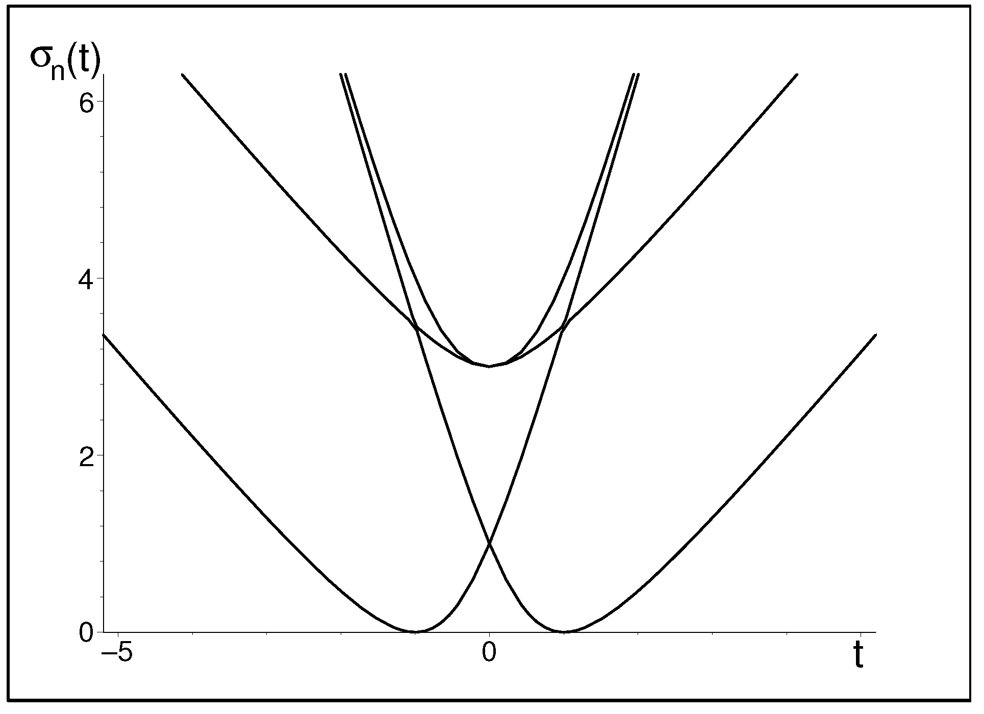
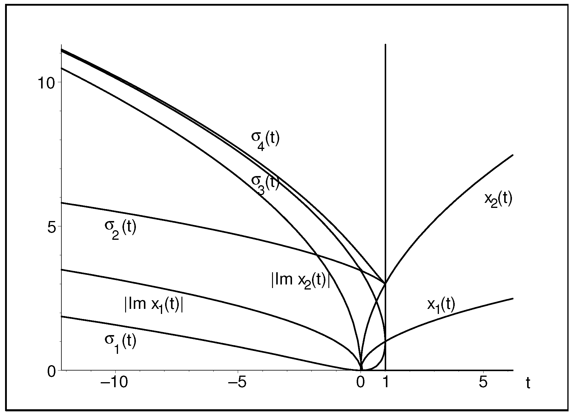
5.1. Four-Grid-Point Simulation of Big Bang

The abstract and general mathematical statements taken from the literature can be complemented by their very explicit algebraic and graphical support. Its first version is provided by the closed-form solvability of the following four-by-four grid-point-operator matrix:

$$X\left(t\right)=\left[\begin{array}{cccc}-3it& \sqrt{3}& 0& 0\\ \sqrt{3}& -it& 2& 0\\ 0& 2& it& \sqrt{3}\\ 0& 0& \sqrt{3}& 3it\end{array}\right]$$

(3)

and by its unitary-equivalent diagonalized avatar $\left(t\right)$ with four non-vanishing elements:

$${}_{11}\left(t\right)=\sqrt{1-t^2}={-}_{44}\left(t\right),{}_{22}\left(t\right)=3\sqrt{1-t^2}={-}_{33}\left(t\right).$$

(4)

Such a structure of the model seems to suggest a suitable underlying symmetry. Unfortunately, any such symmetry (or, perhaps, another elegant explanation of the solvability) is not known yet. In Equation (4), the nice off-diagonal elements emerged as a result of brute-force computer-assisted algebra, as presented in the 2007 paper [30]. In any case, the result yields, after a suitable rescaling of time near $t_{\left(BB\right)}^{\left(EP\right)}=-1$, just an explicit realization of the generic four-level spectrum, as sampled in Figure 1 above. Its Big Collapse alternative near $t_{\left(BC\right)}^{\left(EP\right)}=+1$ is obvious, so it need not be discussed separately.

Once we move to the study of singular values, we find it easy to form the Hermitian-matrix product:

$$\mathbb{X}\left(t\right)=X^{*}\left(t\right)X\left(t\right)=\left[\begin{array}{cccc}9t^2+3& 2it\sqrt{3}& 2\sqrt{3}& 0\\ -2i\sqrt{3}t& 7+t^2& 4it& 2\sqrt{3}\\ 2\sqrt{3}& -4it& 7+t^2& 2it\sqrt{3}\\ 0& 2\sqrt{3}& -2i\sqrt{3}t& 9t^2+3\end{array}\right]$$

and to find the quadruplet of its eigenvalues:

$${\sigma }_{\pm ,\pm }\left(t\right)=5+5t^2\pm 2t\pm 4\sqrt{1-t-t^3+t^4}.$$

Better insight into the shape of these four curves is provided by Figure 7. In contrast to the preceding two-grid-point case, their time dependence ceased to be linear. Still, the bracketing role of these curves remained analogous to the one displayed in Figure 5 and Figure 6 above.

For a verification of the latter observation, interested readers should recall the elementary Formula (4), and insert the real spectrum (=rescaled circles) and/or the absolute values of the imaginary grid points (=rescaled hyperbolas) into Figure 7.

This insertion may also be accompanied by the analogous explicit comments concerning the numerical quality of the bracketing.

Another less obvious observation might concern the closed form of the results. Although the exact formulae for the spectrum itself would survive, in our particular model, at any finite number N of grid points (cf., e.g., [31]), it is not known whether the time dependence of the related singular values remains equally explicit or, at least, qualitatively predictable. This is to be tested now by an explicit computation in what follows.

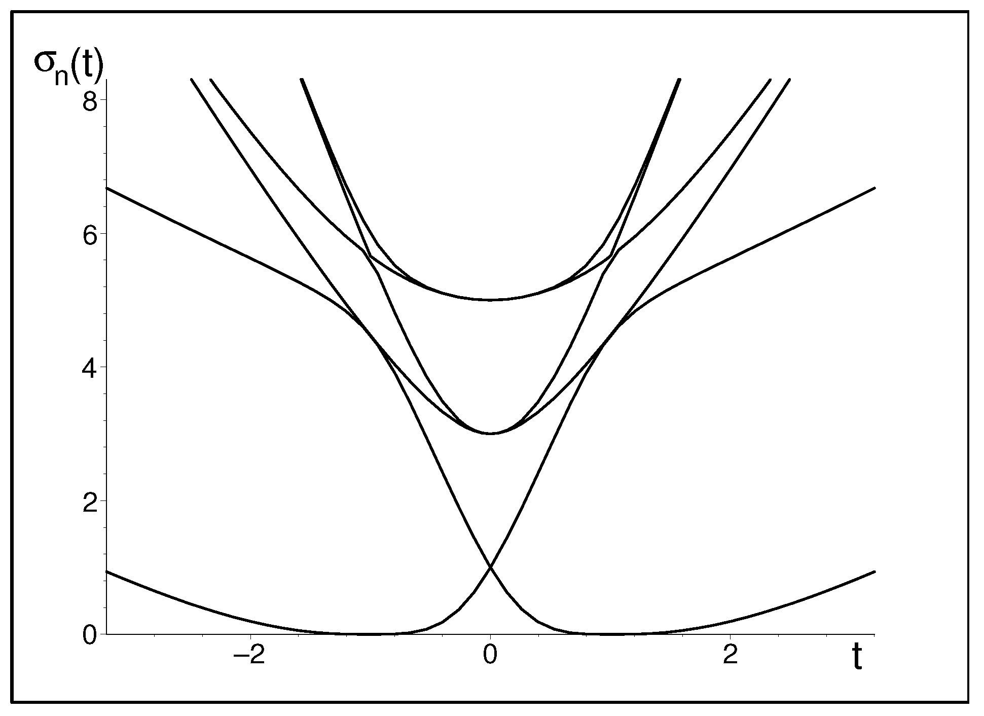
5.2. Six-by-Six Matrix $X\left(t\right)$

Grid-point operator:

$$X\left(t\right)=\left[\begin{array}{cccccc}-5it& \sqrt{5}& 0& 0& 0& 0\\ \sqrt{5}& -3it& 2\sqrt{2}& 0& 0& 0\\ 0& 2\sqrt{2}& -it& 3& 0& 0\\ 0& 0& 3& it& 2\sqrt{2}& 0\\ 0& 0& 0& 2\sqrt{2}& 3it& \sqrt{5}\\ 0& 0& 0& 0& \sqrt{5}& 5it\end{array}\right]$$

(5)

This is still easily diagonalized, yielding the following spectrum:

$${}_{11}\left(t\right)=5\sqrt{1-t^2}={-}_{66}\left(t\right),{}_{22}\left(t\right)=3\sqrt{1-t^2}={-}_{55}\left(t\right),{}_{33}\left(t\right)=\sqrt{1-t^2}={-}_{44}\left(t\right).$$

A fully analogous formula for spectrum holds, after all, at any number of grid points N (see [32]).

Now, the first real challenge comes with the search for the singular values at $N=6$. Once they are defined via eigenvalues of pentadiagonal matrix,

$$\mathbb{X}\left(t\right)=X^{*}\left(t\right)X\left(t\right)=\left[\begin{array}{cccccc}25t^2+5& 2it\sqrt{5}& 2\sqrt{5}\sqrt{2}& 0& 0& 0\\ -2it\sqrt{5}& 13+9t^2& 4it\sqrt{2}& 6\sqrt{2}& 0& 0\\ 2\sqrt{5}\sqrt{2}& -4it\sqrt{2}& 17+t^2& 6it& 6\sqrt{2}& 0\\ 0& 6\sqrt{2}& -6it& 17+t^2& 4it\sqrt{2}& 2\sqrt{5}\sqrt{2}\\ 0& 0& 6\sqrt{2}& -4it\sqrt{2}& 13+9t^2& 2it\sqrt{5}\\ 0& 0& 0& 2\sqrt{5}\sqrt{2}& -2it\sqrt{5}& 25t^2+5\end{array}\right]$$

the goal is only achieved using a computer and a symbolic manipulation software, yielding the six real and non-negative eigenvalues in the form of the well-known Cardano formula.

This means that the result is still available in closed form, but the formula is too long to be displayed here in print. Fortunately, the graphical form of the ultimate set of $N=6$ singular values is still easily obtainable. Moreover, it is important that the form of their time dependence (see Figure 8) remains perfectly analogous to its $N=4$ predecessor.

We have to add that the three branches of the real spectrum of $X\left(t\right)$ at $t\in (-1,1)$ as well as the absolute values of Im $x_n\left(t\right)$ at $t\notin (-1,1)$ are still found localized, asymptotically, inside the three opening wedges, as formed by the singular values in Figure 8. The phenomenon of the bracketing is confirmed.

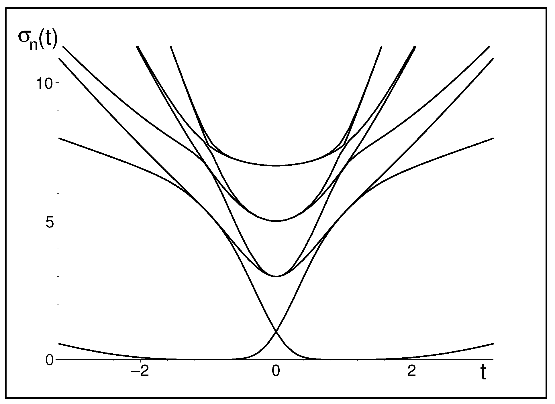
5.3. Eight-by-Eight Matrix $X\left(t\right)$

At any $N<\infty$, the elementary and exactly known (i.e., either purely real or purely imaginary) elements of the spectrum of $X\left(t\right)$ are made mutually different just by a multiplication factor [32]. It would be, therefore, easy to display their time dependence and, if necessary, to insert these spectral curves into the above-displayed graphs of the singular values ${\sigma }_n\left(t\right)$ at $N=4$ and $N=6$. Nevertheless, once we move to the next $N=8$ model,

$$X\left(t\right)=\left[\begin{array}{cccccccc}-7it& \sqrt{7}& 0& 0& 0& 0& 0& 0\\ \sqrt{7}& -5it& 2\sqrt{3}& 0& 0& 0& 0& 0\\ 0& 2\sqrt{3}& -3it& \sqrt{15}& 0& 0& 0& 0\\ 0& 0& \sqrt{15}& -it& 4& 0& 0& 0\\ 0& 0& 0& 4& it& \sqrt{15}& 0& 0\\ 0& 0& 0& 0& \sqrt{15}& 3it& 2\sqrt{3}& 0\\ 0& 0& 0& 0& 0& 2\sqrt{3}& 5it& \sqrt{7}\\ 0& 0& 0& 0& 0& 0& \sqrt{7}& 7it\end{array}\right]$$

(6)

one can still feel pleased by the survival of the existence of the closed-form diagonalizability of the product $\mathbb{X}=X^{*}X=$

$$\left[\begin{array}{cccccccc}49t^2+7& 2it\sqrt{7}& 2\sqrt{7}\sqrt{3}& 0& 0& 0& 0& 0\\ -2i\sqrt{7}t& 19+25t^2& 4it\sqrt{3}& 2\sqrt{3}\sqrt{15}& 0& 0& 0& 0\\ 2\sqrt{7}\sqrt{3}& -4i\sqrt{3}t& 27+9t^2& 2it\sqrt{15}& 4\sqrt{15}& 0& 0& 0\\ 0& 2\sqrt{3}\sqrt{15}& -2i\sqrt{15}t& 31+t^2& 8it& 4\sqrt{15}& 0& 0\\ 0& 0& 4\sqrt{15}& -8it& 31+t^2& 2it\sqrt{15}& 2\sqrt{3}\sqrt{15}& 0\\ 0& 0& 0& 4\sqrt{15}& -2i\sqrt{15}t& 27+9t^2& 4it\sqrt{3}& 2\sqrt{7}\sqrt{3}\\ 0& 0& 0& 0& 2\sqrt{3}\sqrt{15}& -4i\sqrt{3}t& 19+25t^2& 2it\sqrt{7}\\ 0& 0& 0& 0& 0& 2\sqrt{7}\sqrt{3}& -2i\sqrt{7}t& 49t^2+7\end{array}\right]$$

yielding the eight singular values in a form that is easily stored in a computer. This means that the formula for the singular values remains closed and only too long for a printed display. In other words, the time dependence of these characteristics of the $N=8$ system can still be given, very easily, in graphical form, as exemplified in Figure 9, confirming the trends that characterize the present choice of the complex symmetric toy model.

Now, what remains for us to achieve is to perform analogous calculations for another class of grid-point-operator matrices.

6. Another Class of Models: Asymmetric Real Matrices

The main material for our independent test of hypotheses concerning the Big-Bang-related singular values can been found in our older paper [30], in which we managed to illustrate some of the benefits as provided by pseudo-Hermitian quantum theory. For this illustration, we proposed and used certain real asymmetric matrices that appeared exactly solvable at any matrix dimension N.

Let us now show that these matrices could also serve as an illustration of the merits of the use of singular values, still with a particular emphasis upon their applicability and applications in quantum cosmology.

6.1. Two-by-Two $X\left(t\right)$

For the purposes of our present “teaching by example”, it seems to make sense to recall the real-matrix grid-point-operator,

$$X\left(t\right)=\left[\begin{array}{cc}-1& \sqrt{1-t}\\ -\sqrt{1-t}& 1\end{array}\right]$$

(7)

yielding a very natural diagonal-matrix equivalent (i.e., isospectral) avatar,

$$\left(t\right)=\left[\begin{array}{cc}\sqrt{t}& 0\\ 0& -\sqrt{t}\end{array}\right]$$

and possessing a unique exceptional point in the origin, $t^{\left(EP\right)}=0$.

Besides the welcome availability of the closed-form spectrum, it is also easy to form the product

$$\mathbb{X}\left(t\right)=X^{*}\left(t\right)X\left(t\right)=\left[\begin{array}{cc}2-t& -2\sqrt{1-t}\\ -2\sqrt{1-t}& 2-t\end{array}\right]$$

and to diagonalize it:

$$\tilde{\mathbb{X}}\left(t\right)=\left[\begin{array}{cc}2-t+2\sqrt{1-t}& 0\\ 0& 2-t-2\sqrt{1-t}\end{array}\right].$$

Figure 10 now offers a comparison of the two real eigenvalues of $X\left(t\right)$ (existing at $t\ge 0$ and represented by the single right-oriented parabola) with the two singular values of $X\left(t\right)$ (represented, at $t<1$, by the two positive branches of the two left-oriented parabolas).

In the picture, we added a vertical line at $t=1$. This guides our eye to the innocent-looking time $t=1$, beyond which our matrix (7) becomes Hermitian. Although such a “far from Big Bang” time is not too interesting for physics (the model is too elementary), it can serve as an illustration of the existence of a point of change in the overall mathematical paradigm. Beyond this point, indeed, the assumption of the non-Hermiticity is broken, such that, as a consequence, the two singular values degenerate and coincide with one of the eigenvalues, viz., with the positive one. Thus, at $t\ge 1$, one could say that the “bracketing error” is zero. Its specification using singular values becomes redundant but formally exact. In such a Hermitian-matrix regime with $t\ge 1$, practically the same information about the system is carried by the eigenvalues and by the singular values.

Inside the interval of $t\in (t_{\left(BB\right)}^{\left(EP\right)},1)$ (with $t_{\left(BB\right)}^{\left(EP\right)}=0$), the bracketing concerns the real eigenvalues of the non-Hermitian matrix and it has the same form as above.

What is more interesting is the confirmation of the expected bracketing of the absolute value of the complex eigenvalues at $t<0$ (i.e., before the Big Bang). This can be found illustrated in Figure 11. In this regime, the pair of the singular values offers an upper and lower bound of the absolute value of the (incidentally, purely imaginary) eigenvalues.

6.2. Four-by-Four $X\left(t\right)$

The above-mentioned toy-model matrix observables are all real and non-Hermitian but still exactly diagonalizable. For an illustration of their non-numerical algebraic tractability, let us now start from their four-by-four grid-point-operator special case,

$$X\left(t\right)=\left[\begin{array}{cccc}-3& \sqrt{3-3t}& 0& 0\\ -\sqrt{3-3t}& -1& 2\sqrt{1-t}& 0\\ 0& -2\sqrt{1-t}& 1& \sqrt{3-3t}\\ 0& 0& -\sqrt{3-3t}& 3\end{array}\right]$$

(8)

with the closed-form Big-Bang-simulating spectrum,

$$\{-3\sqrt{t},-\sqrt{t},\sqrt{t},3\sqrt{t}\}$$

forming an explicit four-level realization of its generic sample, as displayed in Figure 1.

In parallel with our preceding four-by-four complex symmetric example, it is still comparatively easy to form (though not so easy to display) the product $\mathbb{X}\left(t\right)=X^{*}\left(t\right)X\left(t\right)=$

$$=\left[\begin{array}{cccc}12-3t& -2\sqrt{3-3t}& -2\sqrt{3-3t}\sqrt{1-t}& 0\\ -2\sqrt{3-3t}& 8-7t& -4\sqrt{1-t}& -2\sqrt{3-3t}\sqrt{1-t}\\ -2\sqrt{3-3t}\sqrt{1-t}& -4\sqrt{1-t}& 8-7t& -2\sqrt{3-3t}\\ 0& -2\sqrt{3-3t}\sqrt{1-t}& -2\sqrt{3-3t}& 12-3t\end{array}\right]$$

yielding the following four closed-form eigenvalues after non-numerical diagonalization:

$${\sigma }_{\pm ,\pm }\left(t\right)=10-5t\pm 2\sqrt{1-t}\pm 4\sqrt{{\displaystyle \frac{2\sqrt{1-t}-2t\sqrt{1-t}+t^2\sqrt{1-t}-2+3t-t^2}{\sqrt{1-t}}}}.$$

In spite of its closed form, the latter result is presented much better by a figure. In Figure 12, the attentive readers may find not only the singular values but also, for comparison, both of the standard eigenvalues $x_n\left(t\right)$, which are real for $t>0$ and purely imaginary for $t<0$.

The main point of the message is that at $t<0$ (i.e., before the Big Bang), the picture offers a very nice illustration of the inequalities that represent again the bracketing relations between the singular values and eigenvalues.

6.3. Six-by-Six $X\left(t\right)$

The real and asymmetric six-by-six grid-point-operator matrix,

$$X=\left[\begin{array}{cccccc}-5& \sqrt{5-5t}& 0& 0& 0& 0\\ -\sqrt{5-5t}& -3& 2\sqrt{2-2t}& 0& 0& 0\\ 0& -2\sqrt{2-2t}& -1& 3\sqrt{1-t}& 0& 0\\ 0& 0& -3\sqrt{1-t}& 1& 2\sqrt{2-2t}& 0\\ 0& 0& 0& -2\sqrt{2-2t}& 3& \sqrt{5-5t}\\ 0& 0& 0& 0& -\sqrt{5-5t}& 5\end{array}\right]$$

(9)

is to be recalled, now showing the emergence of the loss of non-numerical solvability. Although the model remains non-numerically solvable for eigenvalues (and the same remains true at any matrix dimension N), the choice of $N=6$ appears to be a boundary, beyond which the evaluation of singular values acquires a more or less numerical character.

A purely formal difficulty even starts when we reveal that, in print, the product $\mathbb{X}=X^{*}X$ appears too large to fit the standard page. We only succeed when we recall the symmetry of this pentadiagonal matrix with respect to both of its diagonals, and display just its abbreviated form:

$$\left[\begin{array}{ccccc}30-5t& -2\sqrt{5-5t}& 2\left(-1+t\right)\sqrt{5}\sqrt{2}& 0& \dots \\ -2\sqrt{5-5t}& 22-13t& -4\sqrt{2-2t}& 6\left(-1+t\right)\sqrt{2}& \ddots \\ 2\left(-1+t\right)\sqrt{5}\sqrt{2}& -4\sqrt{2-2t}& 18-17t& -6\sqrt{1-t}& \ddots \\ 0& 6\left(-1+t\right)\sqrt{2}& -6\sqrt{1-t}& 18-17t& \ddots \\ 0& 0& 6\left(-1+t\right)\sqrt{2}& -4\sqrt{2-2t}& \ddots \\ 0& 0& 0& 2\left(-1+t\right)\sqrt{5}\sqrt{2}& \dots \end{array}\right].$$

Using the computer-assisted algebraic manipulations, we can still deduce a printable secular polynomial:

$$P(x,t)=x^6+\left(70t-140\right)x^5+\left(1743t^2-7728t+7728\right)x^4+$$

$$+\left(18580t^3-142152t^2+314976t-209984\right)x^3+$$

$$+\left(82831t^4-998960t^3+3804720t^2-5611520t+2805760\right)x^2+$$

$$+\left(116550t^5-2191500t^4+13248000t^3-33408000t^2+36864000t-14745600\right)x+50625t^6$$

However, its roots (i.e., the sextuplet of the real and time-dependent eigenvalues of $X\left(t\right)$) can only be localized numerically.

We may conclude that in contrast to its complex predecessor, the alternative real and asymmetric toy model ceases to be suitable for our present methodical purposes at $N\ge 6$.

7. Discussion

7.1. Classical vs. Quantum Gravity in Cosmology

The current state of the relationship between the classical and quantum gravity can briefly be characterized by Thiemann’s words: “despite an enormous effort of work by a vast amount of physicists …we still do not have a credible quantum general relativity theory” because “the problem is so hard” [14]. In this area of research, therefore, one has to appreciate even partial progress. An amendment of the insight in the multiple open problems connected with the quantization of gravity can only be achieved via the detailed technical analyses of certain suitable simplified models.

A few results inspired by these questions were also presented in our present paper. In fact, the background of our considerations can be traced back to Figure 4, indicating that after one makes the most conventional choice of metric $\Theta ={\Theta }_0=I$ (which means that all of the related admissible operators of observables must be Hermitian, ${\Lambda }_0={\Lambda }_0^{†}$ [33]), the existence of any Big-Bang-like degeneracy would be excluded.

Whenever $\Theta =I$, this is a no-go statement that holds unless we impose a suitable ad hoc symmetry. Thus, the typical parameter-dependence of eigenvalues would have the form of avoided crossing. Mathematicians would say that due to the Hermiticity of the operator, the related Kato EP-localizing parameter (i.e., in our models, the time of the Big Bang) must necessarily be complex.

In contrast, after one relaxes the Hermiticity constraint, one finds (or can construct) multiple examples in which $\Theta \ne I$ is nontrivial, and in which the critical EP parameter becomes real. Then, by definition the level-crossing may become exact, unavoided.

One of the scenarios of the later type has constructively been studied, e.g., in [32]. We used there, exclusively, the very special parametric dependence of the EP-supporting spectra as sampled here in Figure 2. By construction, these spectra were guaranteed to be real both before and after passage through the EP singularity. In the picture, one can see a realization of Penrose’s [3] eternally cyclic evolution. By this hypothesis, there exists a sequence of well-separated Aeons of evolution, every one initiated by the Big Bang re-birth of the Universe.

In order to make all of these considerations less speculative and, at the same time, feasible, we turned attention from the spectra to the operators. Emphasis was put on the study of their phenomenological and mathematical aspects. In particular, the conventional construction of eigenvalues was complemented by a less conventional study of singular values. We showed that even the reconstruction of incomplete information carried by the latter quantities enables one to characterize the dynamics of the system even in the anomalous regime near the Big Bang, in which the observability may become lost.

We managed to show that even after the loss of the reality of at least some of the eigenvalues, the singular values themselves remain, by definition, real. From a purely pragmatic point of view, this was shown to open the way towards a reinterpretation of the physics of quantum cosmology in terms of inequalities.

7.2. Quantum Big Bang in Schematic Picture

Due to the enormous complexity of the gravity-quantization challenge, one can notice a sharp contrast between the abstract projects and explicit predictions. One of the decisive specific conceptual obstacles emerging in the quantum theory of gravity near the Big Bang is the necessity of having this theory “background-independent”. This means that, in contrast to relativistic quantum electrodynamics or quantum chromodynamics, one cannot assume the existence of a fixed space–time framework (and perform the quantization of a time- and coordinate-dependent field $\varphi (\overrightarrow{x},t)$) because the geometry of the space–time becomes, by itself, field- and time-dependent [14].

One of the ways out of the dead end has been found in the so-called loop quantum gravity [13]. A consequent background independence is achieved there at the expense of an enormous increase in the complexity of the formalism. Thus, not too surprisingly, even the loop-quantum-gravity-based answers to the rather fundamental question of the existence or non-existence of an initial Big Bang singularity remain ambiguous [9,23].

In such a broad conceptual framework, the essence of the innovation as provided by the present approach is that under certain appropriate mathematical conditions, some of the observables (say, $\Lambda$) may be assigned a physical inner-product metric $\Theta =\Theta (\Lambda )$.

Both $\Lambda$ and $\Theta$ operators can be kept parameter-dependent and, in particular, time-dependent. The formalism seems particularly suitable for the analysis of one of the most important quantum cosmology problems, viz., of the question of compatibility between the classical and quantum notion of the Big Bang.

7.3. Wheeler–DeWitt Equation

Among the numerous existing examples of partial progress, we felt inspired by the observation that in the particular context of quantum cosmology, one of the key points remains “the problem of finding an appropriate inner product on the space of solutions of the Wheeler–DeWitt equation” [15].

The reconstructions of phenomenologically acceptable “physical” inner products for the Wheele-r-DeWitt fields offered deeper new insight into the possible consistent probabilistic interpretation of the canonical gravity in the context of quantum theory in its pseudo-Hermitian operator representation—cf., e.g., [15]. The author of the latter review paper also added that “most of the practical and conceptual difficulties of addressing the …problems for …Wheeler-DeWitt fields can be reduced to, and dealt with, in the context of [a certain] simple oscillator” (cf. section Nr. 3.5 or page 1J.Z. in [15]).

It is needless to add that such a “simple oscillator” was just a schematic, methodically oriented model, not designed to mimic any empirically relevant phenomena. Still, the conceptually innovative pseudo-Hermitian operator nature of the underlying Wheeler’s and DeWitt’s “pseudo-Hermitian Hamiltonians” $H\ne H^{†}$ has to be considered encouraging.

In this sense, our present paper can be also read as an immediate continuation of the two-by-two matrix example, as given in equation Nr. 379 of review [15]. Even more persuasive support of the potential relevance of the present grid-point philosophy could be sought in loc. cit., in the preceding “generic” equation Nr. 377, which is often considered in the partial differential equation form in applications. In such a setting, naturally, one reveals the existence of a certain tension between the discrete grid-point nature of our present models and the continuous-limit essence of the physical reality. Many questions emerge, especially those concerning the optimality of the grid-point lattice near the singularities, etc.

7.4. The Concept of Pseudo-Hermiticity

There exists a specific merit of such an overall theoretical framework which lies in an innovation of the form of information about the observable aspects of the system in question. This information is carried by a pair of operators (thus, let us speak here about $\Lambda$ and $\Theta$) in a way extending the scope of conventional textbooks in which such information is carried just by a single dedicated operator $\Lambda$ called “observable” [34].

The eligible metrics $\Theta$ must be such that the operator product $\Theta \Lambda$ is self-adjoint. A more complete but still concise specification of the necessary mathematics can be found, e.g., in [33]. In this abstract theoretical framework, one of the two information-carrying operators remains to be the conventional one (sampled, e.g., by the Hamiltonian $H={\Lambda }_0$ representing the observable energy in Schrödinger picture). Its new ad hoc partner $\Theta$ (called the physical inner product metric) can be then selected from a fairly large set of suitable, $\Lambda$—compatible candidates.

This is precisely what leads the way towards a mathematically fully consistent presence of an EP singularity in $\Lambda$. In the particular physical quantum Big Bang context, the core of the relevance of a nontrivial operator of a metric (which would coincide with the identity operator in a conventional setting) lies in its variability. Briefly stated, any EP-related degeneracy (and, in particular, the Big Bang spatial degeneracy) can be compensated for, in a properly fine-tuned manner, by a properly adapted $\Theta =\Theta (\Lambda )$ [35].

It is needless to add that the internal consistency of such a basic form of the pseudo-Hermitian quantum theory leads the way towards an extension of its applicability and, in particular, towards the possibility of study, say, of the thermodynamic properties of the Big Bang scenario and/or scenarios. Although these questions already lie beyond the scope of our present paper, investigations can be expected into the concepts of entropy and/or temperature, especially near the EP. One can also expect success in the search for connections of the EP-based theory with the currently quickly developing thermodynamics of black holes, etc.

7.5. Singular Values and Simplifications

In our recent letter [36] devoted to pseudo-Hermiticity-related numerical methods, we proposed a replacement of the study of the complex eigenvalues of operators by the less ambitious search for their singular values. We revealed that these quantities (defined as square roots of eigenvalues of the self-adjoint products $X^{†}X$, i.e., still carrying a significant amount of relevant information about X itself) are all real, so that their numerical localization becomes more easy and user-friendly.

Our present paper describes a number of examples for which the study of singular values remained, in a way motivated by the phenomenology of the Big Bang in cosmology, non-numerical. Sharing the maximally user-friendly tractability by the pure linear algebraic means. In spite of the simplifications (which are, from the point of view of any more realistic consideration, rather drastic), their main merit lies in the insight into the EP-related loss or return of the diagonalizability.

Besides the manifestly non-covariant nature of our toy models, their most efficient simplification should be seen in our replacement of the realistic 3D spatial background with the mere 1D discrete few-grid-point lattice. Its elements are treated as mimicking the evolution of the expanding Universe after the point-like Big Bang at $t=0$.

Such a representation of physical reality does not take into account the dynamics of any energy-momentum-carrying fields because we only introduced to a certain artificial time-dependent spatial geometry that is assumed to be quantized, i.e., treated as a conventional quantum dynamical observable. Every element of the set of spatial grid points is interpreted as a time-dependent eigenvalue of a self-adjoint operator $X\left(t\right)$ acting in Hilbert space $\mathcal{H}$. As an immediate consequence, time t is treated as a mere real parameter without quantum interpretation. Naturally, the time treated as a mere parameter rather than a dynamical coordinate does really oversimplify the intricate relationship between the space–time geometry and the mathematics inherent in quantum gravity (in this respect, see also p. 1292 in [15]). The discretization of the coordinates $x\to x_k$, $k\in \mathbb{N}$ yielded the equidistant and finite grid-point lattice.

Concerning the feasibility of the reinstallation of singularity after quantization, we accepted the philosophy of pseudo-Hermitian quantum mechanics. We revealed that such an approach to realistic cosmology profits from the enhancement of flexibility in model-building processes.

In fact, the main gain appeared to concern the preservation of singularities. In the language of mathematics, the spatial Big Bang degeneracy

$$\underset{t\to t_{BB}}{lim}{x}_k\left(t\right)=x_{BB},\forall k$$

(10)

has been found to be tractable as it reflects the exceptional point value of time.

Another emerging question concerns the differences between the alternative pre-Big-Bang dynamics. This problem was sampled by several pictures, all of which shared the assumption of the reality of the eigenvalues of $X\left(t\right)$ after the Big Bang. In all of them, still, the specific alternative choices of the structure of the pre-Big-Bang era can only be perceived as speculative.

In this respect, we felt inspired by the conventional nuclear, atomic, or molecular physics and by the widely accepted treatment of differences between the so-called closed systems (i.e., stable, bound-state systems) and the so-called open systems (i.e., unstable, resonant quantum systems). In the latter cases, indeed, there exist multiple forms of the comparison of the theory with experiments, with some of them related to the evaluation of the less usual mathematical characteristics of the system, like singular values [25,37].

8. Summary

Once one decides to use Kato’s exceptional points as a means of quantization of classical singularities, the first task that must be fulfilled is a description and classification of the ways of their unfolding. This opens the way towards our understanding of a wealth of quantum phase-transition scenarios ranging from condensed-matter physics up to the cosmology and quantum Big Bang.

A key to our present message lies in the observation that one of the really efficient ways of clarifying an overall mechanism of these unfoldings is provided by the study of elementary non-numerical toy models. Formally, we redirected this study from the conventional analysis of spectra (which are, in general, complex and difficult to localize) to a reduced description of complicated quantum systems in terms of singular values.

The phenomenological context was sampled here by the cosmological Big Bang. The assumption of the existence of a point-like form of such a degeneracy has been shown to lead to direct access to a broad family of new physical quantum-phase-transition-like phenomena. At the same time, multiple new questions have emerged.

The physical motivation of their present analysis was threefold. Firstly, we were impressed by paper [38], which elucidated the connection between the innovative pseudo-Hermitian reformulation of quantum mechanics and the canonical quantization of gravity. This made us believe that a deeper analysis of solvable models can offer the answers to a few relevant methodical as well as conceptual questions.

Secondly, we recalled the pseudo-Hermiticity-related possibility of identification of the quantum phase transitions with the EP-type spectral degeneracies. Although this trick can mostly be found in optics rather than in cosmology [39,40,41], we emphasized that all of the related technicalities could directly be extended to cover the Big-Bang-related phenomena. After all, precisely the same transfer of experience is used in several other branches of physics, ranging from classical optics up to the broad area of atomic, molecular, or nuclear physics [18,25,37].

Thirdly, we revealed that the simulation of a quantized Big Bang could profit from the knowledge of the concept of a singular value. During the formulation of our present project, we felt encouraged by the parallel developments of this topic in mathematics. Quick progress was seen there not only in the abstract EP-related spectral theory of non-Hermitian operators [12,16] but also in its various (e.g., numerical [25,36,42] or theoretical [43]) implementations.

What remains to be particularly appreciated is that in the recent literature, there appears to be a gap between the existence of studies of the unitary evolution channels (i.e., of the corridors in the space of parameters in which the spectrum remains real [32]) and the absence of analogous model-based illustrative descriptions of the EP unfoldings in which the (discrete) spectrum is more general (i.e., complex).

From several complementary points of view, the gap has been partially filled here. In particular, what seems to be truly promising for future research is the progress achieved, via simplified models, in our understanding of operators which lie in a “small” vicinity of an EP singularity. In this vicinity (whatever its “smallness” could mean [44]), the structure of evolution is split into a broad variety of patterns, yielding, sometimes, very specific EP unfoldings. Their bracketing-based classification emerges, which works with singular values and which seems able to distinguish, even in the quantum gravity context, between the conventional unitary evolution scenarios and their resonances-based open-system-like alternatives.

References

1. Tanabashi, M.; Hagiwara, K.; Hikasa, K.; Nakamura, K.; Sumino, Y.; Takahashi, F.; Tanaka, J.; Agashe, K.; Aielli, G.; Amsler, C.; et al. Astrophysical Constants and Parameters. Phys. Rev. D 2019, 98, 030001. [Google Scholar] [CrossRef]
2. Aghanim, N.; Akrami, Y.; Ashdown, M.; Aumont, J.; Baccigalupi, C.; Ballardini, M.; Banday, A.J.; Barreiro, R.B.; Bartolo, N.; Basak, S.; et al. Planck 2018 results. VI. Cosmological parameters. Astron. Astrophys. 2020, 641, A6. [Google Scholar]
3. Gurzadyan, V.G.; Penrose, R. On CCC-predicted concentric low-variance circles in the CMB sky. Eur. Phys. J. Plus. 2013, 128, 22. [Google Scholar] [CrossRef]
4. Znojil, M. Paths of unitary access to exceptional points. J. Phys. Conf. Ser. 2021, 2038, 012026. [Google Scholar] [CrossRef]
5. Borisov, D.I.; Růžička, F.; Znojil, M. Multiply Degenerate Exceptional Points and Quantum Phase Transitions. Int. J. Theor. Phys. 2015, 54, 42934305. [Google Scholar] [CrossRef]
6. Znojil, M. Quantization of Big Bang in crypto-Hermitian Heisenberg picture. In Non-Hermitian Hamiltonians in Quantum Physics; Bagarello, F., Passante, R., Trapani, C., Eds.; Springer: New York, NY, USA, 2016; pp. 383–399. [Google Scholar]
7. Bojowald, M. Absence of a singularity in loop quantum cosmology. Phys. Rev. Lett. 2001, 86, 5227–5230. [Google Scholar] [CrossRef] [PubMed]
8. Rovelli, C. Quantum Gravity; Cambridge University Press: Cambridge, UK, 2004. [Google Scholar]
9. Wang, C.; Stankiewicz, M. Quantization of time and the big bang via scale-invariant loop gravity. Phys. Lett. B 2020, 800, 135106. [Google Scholar] [CrossRef]
10. Kato, T. Perturbation Theory for Linear Operators; Springer: Berlin/Heidelberg, Germany, 1966. [Google Scholar]
11. Mostafazadeh, A. Pseudo-Hermitian quantum mechanics with uynbounded metric operatrors. Phil. Trans. R. Soc. A 2013, 371, 20120050. [Google Scholar] [CrossRef]
12. Pushnitski, A.; Štampach, F. An inverse spectral problem for non-self-adjoint Jacobi matrices. Int. Math. Res. Notices 2024, 2024, 6106–6139. [Google Scholar] [CrossRef]
13. Ashtekar, A.; Lewandowski, J. Background independent quantum gravity: A status report. Class. Quantum Grav. 2004, 21, R53–R152. [Google Scholar] [CrossRef]
14. Thiemann, T. Introduction to Modern Canonical Quantum General Relativity; Cambridge University Press: Cambridge, UK, 2007. [Google Scholar]
15. Mostafazadeh, A. Pseudo-Hermitian Quantum Mechanics. Int. J. Geom. Meth. Mod. Phys. 2010, 7, 1191–1306. [Google Scholar] [CrossRef]
16. Bagarello, F.; Gazeau, J.-P.; Szafraniec, F.; Znojil, M. (Eds.) Non-Selfadjoint Operators in Quantum Physics: Mathematical Aspects; Wiley: Hoboken, NJ, USA, 2015. [Google Scholar]
17. Ju, C.-Y.; Miranowicz, A.; Minganti, F.; Chan, C.-T.; Chen, G.-Y.; Nori, F. Einstein’s Quantum Elevator: Hermitization of Non-Hermitian Hamiltonians via a generalized vielbein Formalism. Phys. Rev. Res. 2022, 4, 023070. [Google Scholar] [CrossRef]
18. Heiss, W.D. Exceptional points—Their universal occurrence and their physical significance. Czech. J. Phys. 2004, 54, 1091–1100. [Google Scholar] [CrossRef]
19. Heiss, W.D. The physics of exceptional points. J. Phys. A Math. Theor. 2012, 45, 444016. [Google Scholar] [CrossRef]
20. Znojil, M. Quantum singularities in a solvable toy model. J. Phys. Conf. Ser. 2024, 29121, 012012. [Google Scholar] [CrossRef]
21. Gurzadyan, V.G.; Penrose, R. CCC and the Fermi paradox. Eur. Phys. J. Plus. 2016, 131, 11. [Google Scholar] [CrossRef]
22. Graefe, E.M.; Günther, U.; Korsch, H.J.; Niederle, A.E. A non-Hermitian PT-symmetric Bose-Hubbard model: Eigenvalue rings from unfolding higher-order exceptional points. J. Phys. A Math. Theor. 2008, 41, 255206. [Google Scholar] [CrossRef]
23. Malkiewicz, P.; Piechocki, W. Turning Big Bang into Big Bounce: II. Quantum dynamics. Class. Quant. Gravity 2010, 27, 225018. [Google Scholar] [CrossRef]
24. Znojil, M. Quasi-Hermitian formulation of quantum mechanics using two conjugate Schroedinger equations. Axioms 2023, 12, 644. [Google Scholar] [CrossRef]
25. Moiseyev, N. Non-Hermitian Quantum Mechanics; Cambridge University Press: Cambridge, UK, 2011. [Google Scholar]
26. Buslaev, V.; Grecchi, V. Equivalence of unstable anharmonic oscillators and double wells. J. Phys. A Math. Gen. 1993, 26, 5541–5549. [Google Scholar] [CrossRef]
27. Bender, C.M.; Boettcher, S. Real spectra in non-Hermitian Hamiltonians having PT symmetry. Phys. Rev. Lett. 1998, 80, 5243. [Google Scholar] [CrossRef]
28. Langer, H.; Tretter, C.H. A Krein space approach to PT symmetry. Czech. J. Phys. 2004, 54, 1113–1120. [Google Scholar] [CrossRef]
29. Albeverio, S.; Kuzhel, S. PT-symmetric operators in quantum mechanics: Krein sopaces methods. In Non-Selfadjoint Operators in Quantum Physics: Mathematical Aspects; Bagarello, F., Gazeau, J.-P., Szafraniec, F., Znojil, M., Eds.; Wiley: Hoboken, NJ, USA, 2015; pp. 283–344. [Google Scholar]
30. Znojil, M. Tridiagonal PT-symmetric N by N Hamiltonians and a fine-tuning of their observability domains in the strongly non-Hermitian regime. J. Phys. A Math. Theor. 2007, 40, 13131–13148. [Google Scholar] [CrossRef]
31. Stoer, J.; Bulirsch, R. Introduction to Numerical Analysis; Springer: New York, NY, USA, 1980. [Google Scholar]
32. Znojil, M. Passage through exceptional point: Case study. Proc. Roy. Soc. A Math. Phys. Eng. Sci. 2020, 476, 20190831. [Google Scholar] [CrossRef]
33. Scholtz, F.G.; Geyer, H.B.; Hahne, F.J.W. Quasi-Hermitian Operators in Quantum Mechanics and the Variational Principle. Ann. Phys. 1992, 213, 74–101. [Google Scholar] [CrossRef]
34. Messiah, A. Quantum Mechanics; North Holland: Amsterdam, The Netherlands, 1961. [Google Scholar]
35. Znojil, M. Quantum phase transitions in nonhermitian harmonic oscillator. Sci. Rep. 2020, 10, 18523. [Google Scholar] [CrossRef] [PubMed]
36. Znojil, M. Complex tridiagonal quantum Hamiltonians and matrix continued fractions. Phys. Lett. A 2025, 551, 130604. [Google Scholar] [CrossRef]
37. Rotter, I. A non-Hermitian Hamilton operator and the physics of open quantum systems. J. Phys. A Math. Theor. 2009, 42, 153001. [Google Scholar] [CrossRef]
38. Mostafazadeh, A.; Zamani, F. Quantum Mechanics of Klein-Gordon fields I: Hilbert space, localized states, and chiral symmetry. Ann. Phys. 2006, 321, 2183–2209. [Google Scholar] [CrossRef]
39. Berry, M.V. Physics of Nonhermitian Degeneracies. Czech. J. Phys. 2004, 54, 1039–1047. [Google Scholar] [CrossRef]
40. Rüter, C.E.; Makris, K.G.; El-Ganainy, R.; Christodoulides, D.N.; Segev, M.; Kip, D. Observation of parity-time symmetry in optics. Nat. Phys. 2010, 6, 192–195. [Google Scholar] [CrossRef]
41. Christodoulides, D.; Yang, J.-K. (Eds.) Parity-Time Symmetry and Its Applications; Springer: Singapore, 2018. [Google Scholar]
42. Fernández, F.M. On a class of non-Hermitian Hamiltonians with tridiagonal matrix representation. Ann. Phys. 2022, 443, 169008. [Google Scholar] [CrossRef]
43. Bagarello, F.; Gargano, F.; Roccati, F. Tridiagonality, supersymmetry and non self-adjoint Hamiltonians. J. Phys. A Math. Theor. 2019, 52, 355203. [Google Scholar] [CrossRef]
44. Bender, C.M.; Dunne, G.V. Large-order perturbation theory for a non-Hermitian PT-symmetric Hamiltonian. J. Math. Phys. 1999, 40, 4616–4621. [Google Scholar] [CrossRef]
Figure 1. The “Big Bang” birth of the Universe, with the expansion of the space sampled by four grid points x n ( t ) (non-covariant classical physics diagram, arbitrary units).
Symmetry 17 00972 g001
Figure 2. Time dependence (i.e., an “unavoided crossing”) of the spatial grid points x n ( t ) during the collapse to a single point (Big Crunch) and subsequent re-birth (Big Bang) of the Universe (classical physics diagram, arbitrary units).
Symmetry 17 00972 g002
Figure 3. A sample of “evolutionary”, time-asymmetric Big Crunch–Big Bang transition (classical physics diagram, arbitrary units).
Symmetry 17 00972 g003
Figure 4. Sample of quantum Big Bounce: Avoided crossing of eigenvalues x n ( t ) of a self-adjoint grid-point operator X ( t ) .
Symmetry 17 00972 g004
Figure 5. A comparison of the time dependence of the real eigenvalues x n ( t ) (=the circle) with the time dependence of the singular values σ n ( s ) (=straight lines) for the two-by-two non-Hermitian toy-model matrix (2). One has a choice here between the Big Bang scenario at t ( B B ) ( E P ) = 1 and the Big Collapse scenario at t ( B C ) ( E P ) = + 1 .
Symmetry 17 00972 g005
Figure 6. The phenomenon of bracketing of the absolute values of the purely imaginary eigenvalues x n ( t ) of matrix (2) by the pairs of singular values σ n ( t ) of the same non-Hermitian matrix at | t | 1 (i.e., in the unstable-solution dynamical regime).
Symmetry 17 00972 g006
Figure 7. Singular values for the complex symmetric four-by-four matrix (3).
Symmetry 17 00972 g007
Figure 8. Singular values for the complex symmetric six-by-six matrix (5).
Symmetry 17 00972 g008
Figure 9. Singular values for the complex symmetric eight-by-eight matrix (6).
Symmetry 17 00972 g009
Figure 10. A comparison of the time dependence of the real eigenvalues x n ( t ) (=the right-looking parabola) with the time dependence of the singular values σ n ( s ) (=two sections of the two left-looking parabolas) for the asymmetric but real matrix (7).
Symmetry 17 00972 g010
Figure 11. Bracketing of the purely imaginary eigenvalues (i.e., of the positive branch of z n ( t ) = Im x n ( t ) ) for the real and asymmetric two-by-two matrix X ( t ) of Equation (7).
Symmetry 17 00972 g011
Figure 12. Bracketing relations for the real and asymmetric four-by-four matrix (8).
Symmetry 17 00972 g012
Disclaimer/Publisher’s Note: The statements, opinions and data contained in all publications are solely those of the individual author(s) and contributor(s) and not of MDPI and/or the editor(s). MDPI and/or the editor(s) disclaim responsibility for any injury to people or property resulting from any ideas, methods, instructions or products referred to in the content.