Distributed Maximum Correntropy Linear Filter Based on Rational Quadratic Kernel Against Non-Gaussian Noise

Abstract

This paper investigates the distributed state estimation problem for the linear system against non-Gaussian noise, where every sensor commutates information only within its adjacent sensors without the need for a fusion center. Correntropy is a similarity metric based on a kernel function that has symmetry. Symmetry means that for any two data points, the output value of the kernel function does not depend on the order of the data points. By adopting a correntropy cost function based on the rational quadratic kernel function approximation to restrain non-Gaussian heavy-tailed noise, a centralized maximum correntropy Kalman filter is first derived for the linear sens+or network system at first. Then the corresponding centralized maximum correntropy information filter is attained by employing the information matrices, which is a foundation for further designing distributed information algorithms under multi-sensor networks. Thirdly, the distributed rational quadratic maximum correntropy information filter and distributed adaptive rational quadratic maximum correntropy information filter are designed by exploiting the weighted census average to solve the non-Gaussian heavy-tailed noise interference in sensor networks. Finally, the performance of the proposed algorithms is illustrated through numerical simulations on the sensor network system.

1. Introduction

The distributed state estimation (DSE) problem has drawn more and more attention in the network domain because the large-scale sensor network is universally employed in various areas, for example target tracking [1,2,3], power systems [4], wireless camera networks [5], and unmanned aerial vehicles [6]. The study of distributed state estimation in various sensor networks has gained wide popularity due to its various advantages over most centralized estimation techniques, such as robustness to individual sensor failures, a low communication burden, expandability to sensor topology variation, and adaptability to modular subsystem adjustments [7]. Dissimilar to the centralized estimation, the distributed approaches do not require the fusion center, where data is interchanged only with the adjacent sensors rather than all the sensors.

Consensus-based methods are one of the most popular DSE algorithms, which are divided into three types [8,9,10,11]. The first type is consensus on estimates (CE) where the consensus average is applied to the predictions or state estimations [12]. The drawback of CE is that it overlooks the information that effectively contains the error covariance, which may result in an underestimation of the uncertainty in the estimation. The second type is consensus on measurements (CM) where the consensus average is employed based on the innovation pairs [13,14]. However, innovation pairs need to be calculated and exchanged in the CM type, which may make the calculation process complex. The third type is consensus on information (CI), which runs a consensus average on the information matrices and information vectors [15]. The consensus on the information matrix and information vector fully utilizes all the information from the state estimation; therefore, the CI type is a bit better compared to the other two types. All of these distributed consensus algorithms are devised on the centralized Kalman filter (CKF) or nonlinear Kalman filter family, which are based on the assumption of the Gaussian noise and employ the minimum mean square error (MMSE) criterion. However, non-Gaussian noise environments, such as heavy-tailed or impulsive noise, are commonly encountered in practical engineering applications, especially for low-cost sensor networks.

Based on the MMSE criterion, several distributed filter algorithms have been employed to deal with the non-Gaussian noise problem; the typical filter methods are the distributed particle filter [16,17,18] and the distributed Gaussian sum filter (GSF) [19]. In distributed particle filtering, each sensor performs local particle filtering and communicates with neighboring sensors to approximate a global estimate, which typically requires a large number of particles. Similarly, in the distributed Gaussian sum filter (GSF), each sensor implements the GSF to generate local estimates. These local estimates, represented by Gaussian components, are merged into a single Gaussian distribution using a moment-matching approach. The resulting merged estimates are then exchanged between neighboring sensors and fused using a weighted Kullback–Leibler divergence. However, a significant limitation of these filters is their high computational cost, which makes them impractical in sensor networks with constrained computational resources.

The performance of distributed state estimation methods can be significantly improved by employing a maximum correntropy criterion (MCC) instead of the aforementioned MMSE criterion, particularly in the presence of non-Gaussian noise disturbances [20,21,22,23]. B. Chen and X. Liu et al. [20] studied a maximum correntropy Kalman filter, which adopts MCC as the optimality criterion instead of using the MMSE to deal with the heavy-tailed impulsive noises. C. Lu and Z. Ren et al. [21] designed a robust recursive filter and smoother based on the cost function induced by the maximum mixture correntropy criterion for nonlinear dynamic models. J. Shao and W. Chen et al. [22] researched an adaptive multi-kernel sized-based maximum correntropy cubature Kalman filter to overcome the excessive convergence problems against non-Gaussian noise. In contrast to the analytical solution of KF or the KF family algorithms, the MCC-based filtering algorithms cannot yield the desired filter gain directly, so an iterative scheme with the Banach fixed-point theory (also named the contraction mapping theory) is proposed to realize the engineering applications. Generally, the Gaussian kernel function is usually employed to build the cost function in the aforesaid MCC-based filter algorithms, whereas the MCC-based filters based the Gaussian kernel function do not always achieve high performance and high robustness due to the difficulty in choosing the optimal kernel function or the appearance of singular matrices, which cause the algorithms to collapse prematurely [24,25]. Therefore, it is crucial to explore alternative types of kernel functions to address the inherent limitations of the Gaussian kernel function during the correntropy applications. The rational quadratic (RQ) kernel function can be regarded as an infinite sum of multiple Gaussian kernels with different characteristic length scales [26,27]. Consequently, the RQ kernel function owns the characters that the underlying function exhibits smooth variations across a range of length scales compared to the Gaussian kernel function [28]. Therefore, it is capable of capturing more intricate and unstable fluctuations in data trends compared to the Gaussian kernel. A challenging attempt has been made by utilizing the rational quadratic kernel function in place of the Gaussian kernel to overcome the shortage of singular matrices [24]. The work in [24] only concentrates on state estimation in a single sensor, and the DSE problem based on the rational quadratic kernel-based correntropy also plays a significant role in large-scale sensor networks. Therefore, the distributed maximum correntropy method based on a rational quadratic kernel function is of great research value and deserves taking time to study it.

In this paper, to further resolve the problem of the appearance of singular matrices and the kernel selection under the heavy-tailed and outliers of non-Gaussian noise in the sensor network system, the adaptive distributed maximum correntropy filter algorithm and its correlated algorithms, which employ the rational quadratic kernel function, are proposed to deal with the DSE problems. The major contributions of this paper are listed as follows:

• The centralized rational quadratic maximum correntropy KF (CRQMCKF) is derived by adopting the correntropy cost function based on the rational quadratic kernel against the non-Gaussian noise for sensor networks.
• The centralized rational quadratic maximum correntropy information filter (CRQMCIF) is derived to address the non-Gaussian noise disturbance, which is the corresponding information style of CRQMCKF.
• The distributed rational quadratic maximum correntropy information filter (DRQMCIF) and the adaptive distributed rational quadratic maximum correntropy information filter (ADRQMCIF) algorithms, by adapting the consensus-weighted average based on the information matrices and information vectors, are acquired to handle the distributed state estimation problem in sensor networks.

The remaining parts of this paper are organized as follows. The relative background knowledge, including correntropy and weighted consensus average, is minutely introduced in Section 2. The CRQMCKF is designed based on the correntropy cost function by exploiting the rational quadratic kernel function, and then, the corresponding CRQMCIF algorithm is obtained through the information matrices; additionally, the DRQMCIF and ADRQMCIF algorithms are acquired by combining the weighted consensus average based on information matrices and information vectors in Section 3. The simulation results are shown in Section 4, which illustrates the robustness and estimation performance of the proposed algorithms. The conclusions are presented in Section 6.

To increase the readability and comprehensibility of the thesis, the nomenclature table in this paper is given.

2. Preliminary

In this section, the preliminaries are summarized separately. At first, the knowledge about correntropy is presented and the rational quadratic kernel function is advanced among the correntropy approximation. Then, the weighted consensus average is introduced to apply in the topology graph in Section 3.

2.1. Correntropy

To enhance the estimation capability of the filter under non-Gaussian noise interference, this paper chooses the maximum correntropy criterion. Correntropy is one of the similarity metrics, which comes from information-theoretic learning [29]. For the two arbitrary random variables $X,Y\in ℝ$ with the joint probability density function (pdf) $p(x,y)$, correntropy is defined as

$$C(X,Y)=E[\kappa (X,Y)]={\displaystyle \iint \kappa (x,y)p(x,y)dxdy},$$

(1)

where $E[\cdot ]$ denotes the expectation operator, and $\kappa (\cdot ,\cdot )$ is a positive definite kernel function satisfying the Mercer theory [30,31]. The kernel function has symmetry. Symmetry means that for any two data points x and y, the output value of the kernel function does not depend on the order of the data points. This is a fundamental property of kernel functions because it reflects the similarity or the symmetry of the inner product.

In general, the joint pdf $p(x,y)$ is mostly unavailable in the practical application. Therefore, $C(X,Y)$ is mostly approximated by the mean estimator as

$$\widehat{C}(X,Y)={\displaystyle \frac{1}{N}}{\displaystyle \sum _{i=1}^N\kappa (x(i),y(i))},$$

(2)

in which ${(x(i),y(i))}_{i=1}^N$ are N sample points extracted from pdf $p(x,y)$. For the kernel selection, there are already different types of methods [20,25,32,33], such as the Gaussian kernel, Student’s t kernel, Cauchy kernel, and Gaussian mixture kernel. In this article, the rational quadratic kernel function is chosen as

$${\kappa }_{RQ}(e)={\left(1+{\displaystyle \frac{||e|{|}^2}{2\alpha b^2}}\right)}^{-\alpha },(e=x-y),$$

(3)

where $\alpha >0$ is a scale mixture parameter, b stands for the length scale of the kernel (i.e., kernel width), and $b>0$. Due to the presence of two coefficients to be determined in Equation (3), it is too complex for practical engineering applications. Currently, single-parameter rational quadratic kernel functions are commonly adopted in the applications and literature on rational quadratic kernel functions [34,35,36]. Thus, single-parameter rational quadratic kernel functions are also utilized in this paper. To be identical to the rational quadratic kernel function in the above-mentioned literature, $\alpha =1$ is chosen in this paper. Then, the rational quadratic kernel function is viewed as

$$k_{RQ}(x,y)=k_{RQ}(e)={\left(1+{\displaystyle \frac{||e|{|}^2}{2b^2}}\right)}^{-1}=1-{\displaystyle \frac{{‖e‖}^2}{{‖e‖}^2+2b^2}},(e=x-y).$$

(4)

The approximation of correntropy taken by the rational quadratic kernel function is expressed as

$$\widehat{C}(X,Y)={\displaystyle \frac{1}{N}}{\displaystyle \sum _{i=1}^N{\kappa }_{RQ}(e(i))},$$

(5)

where $e(i)=x(i)-y(i)$, $i=1,2,\cdots ,N$.

Remark 1. 

For correntropy approximations, the Gaussian kernel function is mostly adopted as the kernel, i.e.,

$$k(x,y)=G_{\sigma }(e)=\exp \left(-{\displaystyle \frac{||e|{|}^2}{2{\sigma }^2}}\right),(e=x-y),$$

(6)

in which σ > 0 represents the Gaussian kernel width. Like the above-mentioned, there are other kernel functions [25,32] and Gaussian mixture kernel functions [33] to be researched.

2.2. Weighted Consensus Average

The topology of the communication graph directly affects the consensus process in distributed filtering algorithms. In large-scale network systems, each node updates its estimate based not only on local measurements but also on information exchanged with its neighbors. The structure of the graph determines how efficiently and reliably information is propagated across the network. Therefore, the communication of a large-scale network system constituted by network sensors is depicted by an undirected connected topology graph $\mathcal{G}=\left(\nu ,E\right)$, in which $\nu =\left\{1,\cdots ,S\right\}$ denotes the set of sensors and $E=\{e_{sd}=(s,d)|s,d\in \nu \}$ is the set of communication links. If $\left(s,d\right)\in E$, the d-th sensor can accept the data transferred from the s-th sensor, which is regarded as a neighborhood of the s-th sensor. Moreover, the neighborhood of the s-th sensor is denoted as ${\mathcal{N}}_s=\left\{d\in \nu |\left(d,s\right)\in E\right\}\cup \left\{s\right\}$, which includes the s-th sensor itself. If other sensors do not establish the link with the s-th sensor, then ${\mathcal{N}}_s=\left\{s\right\}$.

The weighted consensus average algorithm is the widely used distributed method for calculating the mean values. Suppose that every sensor s has an original value $a_s^0$, then each sensor accomplishes the following iteration

$$a_s^l={\displaystyle \sum _{d\in {\mathcal{N}}_s}{\lambda }_{s,d}{a}_d^{l-1}},l=1,2,\cdots ,L-1,$$

(7)

in which l is the consensus iteration number, L is the maximum number of consensus iterations, and L ≥ 2; ${\displaystyle {\sum }_{d\in {\mathcal{N}}_s}{\lambda }_{s,d}}=1$, ${\lambda }_{s,d}\ge 0$; and the weighted consensus matrix $\prod ={({\lambda }_{s,d})}_{S\times S}$ is primitive [37].

When $L\to \infty$, the following equation holds [38,39]

$$a_s^L={\displaystyle \frac{1}{S}}{\displaystyle \sum _{s=1}^S{a}_s^0}.$$

(8)

3. Main Results

In this section, the centralized rational quadratic maximum correntropy Kalman filter is derived for a linear sensor network system at first. Subsequently, the centralized rational quadratic maximum correntropy information filter algorithm is obtained. Then, the distributed rational quadratic information maximum correntropy information filter and the adaptive distributed rational quadratic information maximum correntropy information filter are deduced, which are realized through the weighted average consensus of the information pairs within the information filter.

3.1. Centralized Rational Quadratic Maximum Correntropy Kalman Filter

Consider a linear dynamic system and measurement model with S sensors depicted by

$$x_k={\Phi }_{k-1}{x}_{k-1}+{\omega }_{k-1},$$

(9)

$$z_k^s=H_k^s{x}_k+{\upsilon }_k^s,s=1,\cdots ,S,$$

(10)

where $x_k\in {ℝ}^n$ is the state vector at the k-th time step and $z_k^s\in {ℝ}^m$ is the measurement vector in the s-th sensor at the k-th time step; the state transition matrix ${\Phi }_{k-1}\in {ℝ}^{n\times n}$ and measurement matrix $H_k^s\in {ℝ}^{m\times n}$ are pre-known; ${\omega }_{k-1}\in {ℝ}^n$ and ${\upsilon }_k^s\in {ℝ}^m$ are the mutually independent non-Gaussian process and measurement noise vectors, which have the nominal process noise covariance matrix $Q_{k-1}$ and nominal measurement noise covariance matrix $R_k^s$ for the Kalman family filter algorithm to proceed; and S is the total number of sensors. In the case of $S\ge 2$, the sensors are placed in a distributed way.

Firstly, the CRQMCKF filter algorithm is devised as follows. Under the Kalman-family framework, the CRQMCKF algorithm is comprised of prediction and update. In the prediction, the prior mean vector ${\widehat{x}}_{k|k-1}$ and the covariance matrix ${\mathbf{P}}_{k|k-1}$ are given by

$${\widehat{x}}_{k|k-1}={\Phi }_{k-1}{\widehat{x}}_{k-1|k-1},$$

(11)

$${\mathbf{P}}_{k|k-1}={\Phi }_{k-1}{\mathbf{P}}_{k-1}{\Phi }_{k-1}^T+Q_{k-1}.$$

(12)

The Cholesky decomposition of ${\mathbf{P}}_{k|k-1}$ and ${\mathbf{R}}_k^s$ are written as

$$B_p{B}_p^T={\mathbf{P}}_{k|k-1},B_{r,s}{(B_{r,s})}_T=R_r^s.$$

(13)

To deal with non-Gaussian interference, the cost function is adopted by correntropy based on the rational-quadratic kernel as

$${\mathcal{J}}_{RQ}(x_k)={\displaystyle \frac{1}{n+m}}\left({\displaystyle \sum _{i=1}^n{k}_{RQ}(e_x^i)}+{\displaystyle \sum _{j=1}^m{\displaystyle \sum _{s=1}^S{k}_{RQ}(e_{z,s}^j)}}\right),$$

(14)

where $k_{RQ}(\cdot )$ is rational quadratic function described by Equation (4). Additionally, $e_x^i$ $(i=1,\cdots ,n)$ and $e_{z,s}^j$ $(j=1,\cdots ,m)$ are the i-th and the j-th element of the vectors $e_x$ and $e_{z,s}$

$$e_x=B_p^{-1}(x_k-{\widehat{x}}_{k|k-1}),$$

(15)

$$e_{z,s}={(B_r^s)}^{-1}(z_k^s-H_k^s{x}_k),s=1,2,\cdots ,S.$$

(16)

The state solution ${\widehat{x}}_{k|k}$ is to maximize the above cost function utilizing all sensors’ measurements based on the maximum correntropy criterion (MCC)

$${\widehat{x}}_{k|k}=\underset{x_k}{\arg \max }{\mathcal{J}}_{RQ}(x_k).$$

(17)

The optimal state estimate can be acquired by

$${\displaystyle \frac{\partial {\mathcal{J}}_{RQ}(x_k)}{\partial x_k}}=0.$$

(18)

Equation (18) can be further shown by

$$\begin{array}{l}-{\displaystyle \frac{1}{2b^2}}{\displaystyle \sum _{i=1}^n{k}_{RQ}^2(e_x^i)B_{p,i}^{-T}{B}_{p,i}^{-1}(x_k-{\widehat{x}}_{k|k-1})}\\ \hspace{1em}+{\displaystyle \frac{1}{2b^2}}{\displaystyle \sum _{j=1}^m{\displaystyle \sum _{s=1}^S{k}_{RQ}^2(e_{z,s}^j){(H_k^s)}^T{B}_{r,s,j}^{-T}{B}_{r,s,j}^{-1}(z_k^s-H_k^s{x}_k)}}=0\end{array}$$

(19)

where $B_{p,i}$ $(i=1,\cdots ,n)$ and $B_{r,s,j}$ $(j=1,\cdots ,m)$ are the i-th and the j-th row of the matrixes $B_p$ and $B_{r,s}$, respectively.

The matrix form of Equation (19) is expressed as

$$B_p^{-T}{C}_x{B}_p^{-1}(x_k-{\widehat{x}}_{k|k-1})={\displaystyle \sum _{s=1}^S{(H_k^s)}^T{(B_{r,s})}^{-T}{C}_z^s{(B_{r,s})}^{-1}(z_k^s-H_k^s{x}_k)},$$

(20)

in which

$$C_x=\mathrm{diag}(k_{RQ}^2(e_{x,1}),\cdots ,k_{RQ}^2(e_{x,n})),$$

(21)

$$C_z^s=\mathrm{diag}(k_{RQ}^2(e_{z,1}^s),\cdots ,k_{RQ}^2(e_{z,m}^s)).$$

(22)

Let

$$\begin{array}{l}{\overline{P}}_{k|k-1}=B_p{C}_x^{-1}{B}_p^T,\\ {\overline{R}}_k^s=B_r^s{(C_z^s)}^{-1}{(B_r^s)}^T.\end{array}$$

(23)

According to the symbolism (23), Equation (20) can be expressed as

$$\left({\overline{P}}_{k|k-1}^{-1}+{\displaystyle \sum _{s=1}^S{(H_k^s)}^T{({\overline{R}}_k^s)}^{-1}{H}_k^s}\right)x_k={\overline{P}}_{k|k-1}^{-1}{\widehat{x}}_{k|k-1}+{\displaystyle \sum _{s=1}^S{(H_k^s)}^T{({\overline{R}}_k^s)}^{-1}{z}_k^s}.$$

(24)

Adding and subtracting ${\displaystyle \sum _{s=1}^s{(H_k^s)}^T{({\overline{R}}_k^s)}^{-1}{H}_k^s}{\widehat{x}}_{k|k-1}$ on the right side of the Equation (24)

$$\begin{array}{l}\left({\overline{P}}_{k|k-1}^{-1}+{\displaystyle \sum _{s=1}^S{(H_k^s)}^T{({\overline{R}}_k^s)}^{-1}{H}_k^s}\right)x_k\\ =\left({\overline{P}}_{k|k-1}^{-1}+{\displaystyle \sum _{s=1}^S{(H_k^s)}^T{({\overline{R}}_k^s)}^{-1}{H}_k^s}\right){\widehat{x}}_{k|k-1}+{\displaystyle \sum _{s=1}^S{(H_k^s)}^T{({\overline{R}}_k^s)}^{-1}(z_k^s-H_k^s{\widehat{x}}_{k|k-1})}.\end{array}$$

(25)

Multiplying ${\left({\overline{P}}_{k|k-1}^{-1}+{\displaystyle \sum _{s=1}^S{(H_k^s)}^T{({\overline{R}}_k^s)}^{-1}{H}_k^s}\right)}^{-1}$ on both sides of Equation (25), then the state estimation ${\widehat{x}}_{k|k}$ can be obtained as the following (See Appendix A):

$${\widehat{x}}_{k|k}={\widehat{x}}_{k|k-1}+{\overline{K}}_k({\overline{z}}_k-{\overline{H}}_k{\widehat{x}}_{k|k-1}),$$

(26)

where ${\overline{z}}_k$ is stacked measurement vector and defined as

$${\overline{z}}_k={\left[{\left(z_k^1\right)}^T,{\left(z_k^2\right)}^T,\cdots ,{\left(z_k^S\right)}^T\right]}^T,$$

(27)

${\overline{H}}_k$ is a stacked measurement matrix of all sensors and expressed as

$${\overline{H}}_k={\left[{\left(H_k^1\right)}^T;{\left(H_k^2\right)}^T;\cdots ;{\left(H_k^S\right)}^T\right]}^T.$$

(28)

${\overline{K}}_k$ is the gain matrix, which is given as

$${\overline{K}}_k={\left({\overline{P}}_{k|k-1}^{-1}+{\overline{H}}_k^T{\overline{R}}_k^{-1}{\overline{H}}_k\right)}^{-1}{\overline{H}}_k^T{\overline{R}}_k^{-1},$$

(29)

in which

$${\overline{R}}_k=\mathrm{diag}({\overline{R}}_k^1,{\overline{R}}_k^2,\cdots ,{\overline{R}}_k^S).$$

(30)

${\overline{K}}_k$ is also rewritten as

$${\overline{K}}_k={\overline{P}}_{k|k-1}{\overline{H}}_k^T{\left({\overline{R}}_k+{\overline{H}}_k{\overline{P}}_{k|k-1}{\overline{H}}_k^T\right)}^{-1}.$$

(31)

The detailed derivation of Equation (31) can be seen in Appendix B.

The state error covariance matrix $P_{k|k}$ can be calculated by

$$P_{k|k}=(I-{\overline{K}}_k{\overline{H}}_k)P_{k|k-1}{(I-{\overline{K}}_k{\overline{H}}_k)}^{\mathrm{T}}+{\overline{K}}_k{R}_k{\overline{K}}_k^{\mathrm{T}}.$$

(32)

The CRQMCKF algorithm is outlined in Algorithm 1.

Algorithm 1 Centralized rational quadratic maximum correntropy Kalman filter (CRQMCKF)

$\mathrm{Initialization}: x_{0|0}={\widehat{x}}_0$$, {\mathbf{P}}_{0|0}={\mathbf{P}}_0$; For k = 1, 2, 3, …, do $\mathrm{Prediction}: \mathrm{update} {\widehat{x}}_{k|k-1}$$\mathrm{and} {\mathbf{P}}_{k|k-1}$ based on Equations (11) and (12); $\mathrm{Update}: \mathrm{Select} \mathrm{the} \mathrm{kernel} \mathrm{width} b, \mathrm{using} \mathrm{Equations} (13), \mathrm{Equations} (15) \mathrm{and} (16),$ $\mathrm{Equations} (21)\text{–}(23), \mathrm{Equations} (26)\text{–}(32) \mathrm{to} \mathrm{calculate} {\widehat{x}}_{k|k}$$\mathrm{and} P_{k|k}$;

Remark 2. 

Compared to the conventional centralized Kalman filter (CKF), the proposed CRQMCKF algorithm introduces  $C_x$ and  $C_z^s$ for the s-th sensor to modify the estimation performance, which is changed according to deformation ($e_{x,i}$ in Equation (15) and  $e_{z,j}^s$ in Equation (16)) of the one-step predict errors and every sensor’s innovation by the kernel width b. When the model is disturbed by large errors,  $C_x$ and  $C_z^s$ would reduce and decay according to an inverse proportional function in Equation (4) (the rational quadratic function in Equation (4) can be identically deformed to  $k_{RQ}(x,y)=2b^2/{‖e‖}^2+2b^2$, which is a translation of the inverse proportional function and has the same graph trend as the inverse proportional function). Mathematically, the rational quadratic function decays much slower than the exponential function, so  $C_x$ and $C_z^s$ are not easily equal to zero when the large outlier or pulse noise arises. This character can avoid the singular matrices under the computer precision requirements for multi-dimensional variables. Peculiarly, when $e_{x,i}\to \infty ,e_{z,j}^s\to \infty$, then  $C_x\to 0$ and  $C_z^s\to 0$, the proposed algorithm ends early, which illustrates that this algorithm can voluntarily avoid the bad influence of abnormal errors, which are produced by system or measurement outliers.

Remark 3. 

The kernel width b has a significant impact on the algorithm estimation effect. When the kernel width b is too small, the estimation performance of the algorithm does not improve and sometimes even decreases, because the rational quadratic function values tend to zero and do not act as a regulator, whereas a large kernel width b makes the CRQMCKF algorithm converge to the centralized Kalman filter. Specially,  $C_x\to I_n$ and $C_z^s\to I_m$ when the kernel width $b\to \infty$, which means that CRQMCKF tends to CKF.

3.2. Centralized Rational Quadratic Maximum Correntropy Information Filter

To acquire the information form of the above CRQMCKF algorithm, like the standard centralized information filter (CIF), some approximation method in the derivations is adopted.

The step of prediction is the same as the above CRQMCKF algorithm. To obtain the information form of the state update, consider the information matrix $Y_{k|k}$ as the following

$$Y_{k|k}=P_{k|k}^{-1}=P_{k|k-1}^{-1}+{\overline{H}}_k^T{\overline{R}}_k^{-1}{\overline{H}}_k=P_{k|k-1}^{-1}+{\displaystyle \sum _{s=1}^S{(H_k^s)}^T{({\overline{R}}_k^s)}^{-1}{H}_k^s}\triangleq Y_{k|k-1}+{\displaystyle \sum _{s=1}^S{U}_k^s},$$

(33)

where the one-prediction information matrix $Y_{k|k-1}$ and the information matrix increment $U_k^s$ are denoted as

$$Y_{k|k-1}=P_{k|k-1}^{-1},$$

(34)

$$U_k^s={(H_k^s)}^T{({\overline{R}}_k^s)}^{-1}{H}_k^s.$$

(35)

Let $y_{k|k}=Y_{k|k}{\widehat{x}}_{k|k}$ is the estimation information vector. Multiplying $Y_k$ on both ends of Equation (26),

$$\begin{array}{ll}{y}_{k|k}& =Y_{k|k}{\widehat{x}}_{k|k}=[P_{k|k-1}^{-1}+{\overline{H}}_k^T{\overline{R}}_k^{-1}{\overline{H}}_k][{\widehat{x}}_{k|k-1}+{\overline{K}}_k({\overline{z}}_k-{\overline{H}}_k{\widehat{x}}_{k|k-1})]\\ & =P_{k|k|d-1}^{-1}{\widehat{x}}_{k|k-1}+{\overline{H}}_k^T{\overline{R}}_k^{-1}{\overline{H}}_k{\widehat{x}}_{k|k-1}+[P_{k|k|d-1}^{-1}+{\overline{H}}_k^T{\overline{R}}_k^{-1}{\overline{H}}_k]{\overline{K}}_k({\overline{z}}_k-{\overline{H}}_k{\widehat{x}}_{k|k-1})\\ & =P_{k|k|d-1}^{-1}{\widehat{x}}_{k|k-1}+{\overline{H}}_k^T{\overline{R}}_k^{-1}{\overline{H}}_k{\widehat{x}}_{k|k-1}+{\overline{H}}_k^T{\overline{R}}_k^{-1}({\overline{z}}_k-{\overline{H}}_k{\widehat{x}}_{k|k-1})\\ & =P_{k|k|d-1}^{-1}{\widehat{x}}_{k|k-1}+{\overline{H}}_k{\overline{R}}_k^{-1}{\overline{z}}_k=P_{k|k|d-1}^{-1}{\widehat{x}}_{k|k-1}+{\displaystyle \sum _{s=1}^S{(H_k^s)}^T{({\overline{R}}_k^s)}^{-1}{z}_k^s}\\ & \triangleq y_{k|k-1}+{\displaystyle \sum _{s=1}^S{u}_k^s},\end{array}$$

(36)

where the one-prediction information vector $y_{k|k-1}$ and the information vector increment $u_{s,k}$ are given as

$$y_{k|k-1}=Y_{k|k-1}{\widehat{x}}_{k|k-1},$$

(37)

$$u_k^s={(H_k^s)}^T{({\overline{R}}_k^s)}^{-1}{z}_k^s.$$

(38)

The detailed deducing process can be seen in Appendix C.

The CRQMCIF algorithm is summarized in Algorithm 2.

Algorithm 2 Centralized rational quadratic maximum correntropy information filter (CRQMCIF)

$\mathrm{Initialization}: \mathrm{Let} x_{0|0}={\widehat{x}}_0$$, {\mathbf{P}}_{0|0}={\mathbf{P}}_0$$, \mathrm{then} Y_0=P_{0|0}^{-1}$$\mathrm{and} y_0=Y_0{\widehat{x}}_0$; For k = 1, 2, 3, …, do $\hspace{1em}\mathrm{Prediction}: \mathrm{update} Y_{k|k-1}$$\mathrm{and} y_{k|k-1}$ by Equations (34) and (37); $\hspace{1em}\mathrm{Update}: \mathrm{Calculate} Y_{k|k}$$\mathrm{and} y_{k|k}$ based on Equations (33) and (36); $\hspace{1em}\mathrm{Calculate} {\widehat{x}}_{k|k}$$\mathrm{by} {\widehat{x}}_{k|k}={(Y^{k|k})}^{-1}{y}_{k|k}$; End.

Remark 4. 

From (21) and (22), when the kernel width b → ∞,$C_x\to I_n,C_z^s\to I_m$, the estimation of CRQMCIF is similar to that of the standard CIF algorithm, for which the effects are equivalent to the CKF and CRQMCKF; when the  $C_x\to 0$, $C_z^s\to 0$, the estimation of CRQMCIF is only time prediction, which is the same as CRQMCKF. In general, as shown in the simulation outcome in Section 4.4, the estimation performance of CRQMCIF and CRQMCKF is similar.

3.3. Distributed Rational Quadratic Maximum Correntropy Information Filter

To effectively obtain the DRQMCIF, the weighted consensus average is introduced to calculate the weighted sum of the information matrix increment Equation (35) and the information vector increment Equation (38), respectively. Particularly, each sensor is given the same initial value ${\widehat{x}}_0$ and ${\mathbf{P}}_0$, and thus $Y_{0|0}^s=P_0^{-1}$ and $y_{0|0}^s=Y_{0|0}^s{\widehat{x}}_0$ for all the sensors s (s = 1, 2,…, S) in the distributed algorithm. The initial value of the information matrix increment $U_k^{s,0}=U_k^s$ and information vector increment initialization $u_k^{s,0}=u_k^s$ selects the information increment form of CRQMCIF in Equations (35) and (38), which indicates the information increment items of the s-th sensor at the k-th time after the l-th consensus iteration. Applying the method in Equation (7) to perform the weighted consensus average, thus, the iterative information matrix increment $U_k^{s,l}$ and information vector increment $u_k^{s,l}$ is acquired as

$$\left\{\begin{array}{l}{U}_k^{s,l}={\displaystyle \sum _{d\in {\mathcal{N}}_s}{\lambda }_{s,d}{U}_k^{s,l-1}},\\ u_k^{s,l}={\displaystyle \sum _{d\in {\mathcal{N}}_s}{\lambda }_{s,d}{u}_k^{s,l-1}}.\end{array}\right.$$

(39)

where $l\in [1,L]$ is the number of consensus iterations, ${\lambda }_{s,d}\ge 0$ is the consensus weight value, and ${\displaystyle {\sum }_{d\in \mathcal{N}}{\lambda }_{s,d}}=1$. In this paper, the weighted consensus matrix is built based on the Metropolis weights, which are given as

$${\lambda }_{s,d}=\left\{\begin{array}{ll}1/(1+\max \{l_s,l_d\}),& \mathrm{if} \{s,d\}\in \nu ;\\ 1-{\displaystyle {\sum }_{\{s,d\}\in \nu }{\lambda }_{s,d}},& \mathrm{if} s=d;\\ 0,& \mathrm{otherwise}.\end{array}\right.$$

(40)

in which $l_s=|{\mathcal{N}}_s|$ represents the degree of the s-th sensor in the sensor network communication topology diagram.

From Equation (40), the Metropolis weight matrix $\mathrm{\Gamma }={({\lambda }_{s,d})}_{S\times S}$ is row stochastic and primitive, then $U_k^{s,L}$ and $u_k^{s,L}$ would respectively converge to the mean value of $U_k^s$ and $u_k^s$ when the total consensus iterative number L→∞, i.e.,

$$\left\{\begin{array}{l} \underset{L\to \infty }{\lim }{U}_k^{s,L}={\displaystyle \frac{1}{S}}{\displaystyle \sum _{s=1}^S{U}_k^s},\\ \underset{L\to \infty }{\lim }{u}_k^{s,L}={\displaystyle \frac{1}{S}}{\displaystyle \sum _{s=1}^S{u}_k^s},\end{array}\right.$$

(41)

which implies that the weight consensus average method could circuitously transmit localized information throughout the overall network.

After the weighted consensus averaging step, each sensor independently updates its information matrix and information vector through data transmitted from the neighboring sensor. Specifically, the information matrix and information vector are updated as follows:

• Update of the Information Matrix: The information matrix $Y_{k|k}^s$ for each sensor s at the k-th time step is computed by adding the weighted average increment of the information matrix ${\varpi }_k^s{U}_k^{s,l}$ obtained after L rounds of consensus iterations to the information matrix at the previous time step $Y_{k|k-1}^s$. This updating process encapsulates the integration of information exchanged between sensors and reflects the consensus gradually achieved during the iterative process.

  $$Y_{k|k}^s=Y_{k|k-1}^s+{\varpi }_k^s{U}_k^{s,L},$$

  (42)

  in which ${\varpi }_k^s=S$ for $L\ge 2$; when L = 1, let ${\varpi }_k^s=1$, which implies that each sensor simply accomplishes one local CRQMCIF employing the information transmitted by its linked sensors.
• Update of the Information Vector: Similarly, the information vector $y_{k|k}^s$ for the s-th sensor at the k-th time step is updated by adding the corresponding consensus averaged information vector increment ${\varpi }_k^s{u}_k^{s,l}$ to the estimate at the previous time step $y_{k|k-1}^s$. This ensures that the state estimation vector incorporates a collective understanding of the observed data after the consensus process. $y_k^s$ is expressed by

  $$y_{k|k}^s=y_{k|k-1}^s+{\varpi }_k^s{u}_k^{s,L},$$

  (43)

  where ${\varpi }_k^s$ is the same as described above.

The DRQMCIF algorithm is outlined in Algorithm 3.

Algorithm 3 Distributed rational quadratic maximum correntropy information filter (DRQMCIF)

$\mathrm{Initialization}: \mathrm{Each} \mathrm{sensor} s (s=1, 2, \cdots , S) \mathrm{is} \mathrm{given} \mathrm{initial} \mathrm{value} x_{0|0}^s={\widehat{x}}_0$$, {\mathbf{P}}_{0|0}^s={\mathbf{P}}_0,$ $\hspace{1em}\hspace{1em}\hspace{1em}\hspace{1em}\hspace{1em}\hspace{1em}\mathrm{calculate} \mathrm{information} \mathrm{matrix} Y_{0|0}^s=P_0^{-1}$$\mathrm{and} \mathrm{information} \mathrm{vector} y_{0|0}^s=Y_{0|0}^s{\widehat{x}}_{0|0}$; For k = 1, 2, 3, …, n $\hspace{1em}\hspace{1em}\hspace{1em}\mathrm{Calculate} U_k^{s,0}$$\mathrm{and} u_k^{s,0}$ by Equations (35) and (38); $\hspace{1em}\hspace{1em}\hspace{1em}\mathrm{Complete} \mathrm{the} \mathrm{consensus} \mathrm{average} \mathrm{by} \mathrm{Equation} (39) \mathrm{for} l=1,2,\cdots ,L$ based on the Metropolis weight Equation (40); $\hspace{1em}\hspace{1em}\hspace{1em}\mathrm{Calculate} Y_{k|k}^s$$\mathrm{and} y_{k|k}^s$ based on Equations (42) and (43); $\hspace{1em}\hspace{1em}\hspace{1em}\mathrm{Calculate} {\widehat{x}}_{k|k}^s$$\mathrm{by} {\widehat{x}}_{k|k}^s={(Y_{k|k}^s)}^{-1}{y}_{k|k}^s$; End.

In distributed Algorithm 3, each sensor simply communicates with the neighbor sensors, which is ideal for low-cost sensors with finite communication capabilities. For every time interval k, each sensor s completes L consensus iterations. In the practice application, the estimation effect of DRQMCIF approaches that of CRQMCIF. For L→∞, there is the following conclusion.

Theorem 1. 

For the undirected linked sensor network, the weights consensus matrix $\mathrm{\Gamma }={({\lambda }_{s,d})}_{S\times S}$ is a right random matrix, i.e., ${\displaystyle {\sum }_{d\in {\mathcal{N}}_s}{\lambda }_{s,d}}=1$, ${\lambda }_{s,d}\ge 0$ for $s=1,2,\cdots ,S$. And $\mathrm{\Gamma }$ is primitive; that is, there exists a positive integer k, satisfying ${\mathrm{\Gamma }}^k>0$. When the iterative number L→∞, the DRQMCIF can attain the same estimation effect as the CRQMCIF.

Proof. 

See Appendix D. □

3.4. Adaptive Distributed Rational Quadratic Maximum Correntropy Information Filter

The kernel width of the rational quadratic kernel function plays a magnificent role in the convergence speed of the MCC-family algorithm. When other parameters are changeless, an extremely small kernel width affects the convergence and stability, and even the steady-state error may become larger. However, a particularly large kernel width reduces the rate of convergence and estimation performance. There is no way to obtain the theoretical optimal kernel width in the current research works. Thus, an adaptive adjustable kernel width is one of the popular manners to be selected to resolve this problem.

An online recursion design is enforced to update the kernel width in the MCC-family algorithm. Herein, the kernel width is designed as follows to enable the measurement-specific treatment of outliers

$$b_{j,k}^s={\mu }_{j,k}^s\cdot b_{\max },$$

(44)

where ${\mu }_{j,k}^s$ is the adaptive coefficient in the j-th element of measurement at the k-th step for the s-th sensor; $b_{\max }$ is the presetting kernel width. The innovation vector at the s-th sensor is defined by

$${\tilde{z}}_k^s=z_k^s-{\widehat{z}}_{k|k-1}^s=z_k^s-H_k^s{\widehat{x}}_{k|k-1}=H_k^s{x}_k+{\upsilon }_k^s-H_k^s{\widehat{x}}_{k|k-1}=H_k^s{\tilde{x}}_{k|k-1}+{\upsilon }_k^s.$$

(45)

To detect the measurement outliers, the innovation vector covariance matrix is acquired by

$$P_{zz,k|k-1}^s=E[{\tilde{z}}_k^s{({\tilde{z}}_k^s)}^T]=E[(H_k^s{\tilde{x}}_{k|k-1}+{\upsilon }_k^s){(H_k^s{\tilde{x}}_{k|k-1}+{\upsilon }_k^s)}^T]=H_k^s{\mathbf{P}}_{k|k-1}{(H_k^s)}^T+R_k^s,$$

(46)

and ${\beta }_{j,k}^s$ is chosen as the following

$${\beta }_{j,k}^s={\displaystyle \frac{\tau \cdot P_{zz,j,k|k-1}^s}{{({\tilde{z}}_{j,k}^s)}^2}},$$

(47)

where $P_{zz,j,k|k-1}^s$ is the j-th diagonal element of $P_{zz,k|k-1}^s$, ${\tilde{z}}_{j,k}^s$ is the j-th element of ${\tilde{z}}_k^s$, and $\tau$ is the confidence level factor, which is set based on the chi-square distribution with a single degree of freedom.

The adaptive coefficient ${\mu }_{j,k}^s$ is devised by

$${\mu }_{j,k}^s={\displaystyle \frac{{‖{\beta }_{j,k}^s‖}^2}{{‖{\beta }_{j,k}^s‖}^2+2b_{\max }^2}}={\displaystyle \frac{1}{1+2b_{\max }^2/{‖{\beta }_{j,k}^s‖}^2}},$$

(48)

where ${\mu }_{j,k}^s\in (0,1)$ is bounded and positive. The adaptive kernel width is obtained by substituting Equation (48) into Equation (44).

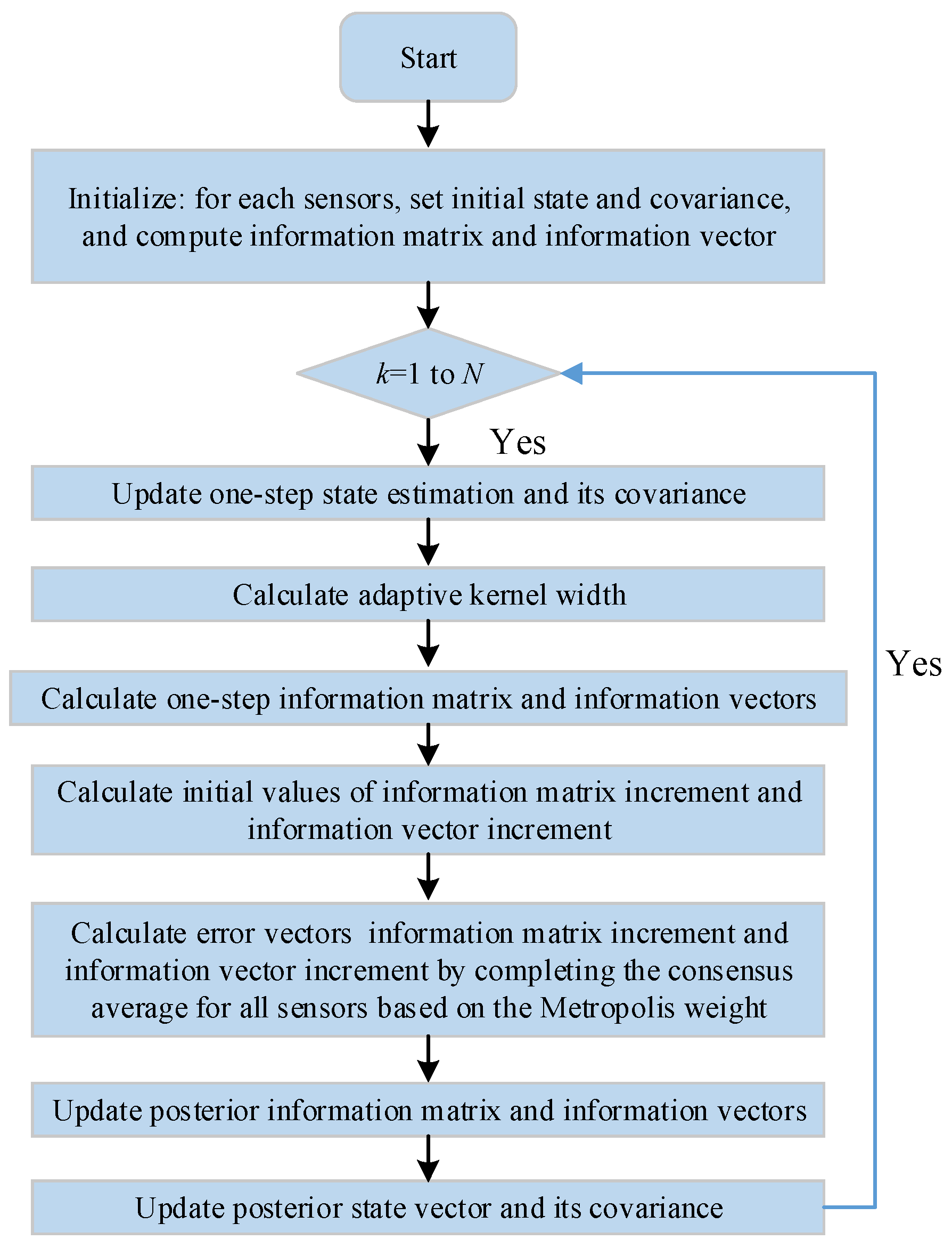
The ADRMCIF algorithm is listed in Algorithm 4.

Remark 5. 

When the measurement noise is Gaussian noise,  ${({\tilde{z}}_{j,k}^s)}^2$ would be smaller than $\tau \cdot P_{zz,j,k|k-1}^s$, ${\beta }_{j,k}^s$ is large. Under this circumstance, the adaptive coefficient ${\mu }_{j,k}^s$ becomes larger from Equation (48), which indicates that the kernel width is restructured to keep it large to ensure higher estimation precision. Meanwhile, conversely, when the measurement noise encounters the outliers, ${({\tilde{z}}_{j,k}^s)}^2$ would be prominently larger than $\tau \cdot P_{zz,j,k|k-1}^s$, ${\beta }_{j,k}^s$ will be smaller. In this case, the adaptive coefficient ${\mu }_{j,k}^s$ becomes smaller, which forces the correntropy value to reduce to zero to eliminate the influence of outliers.

Algorithm 4 Adaptive distributed rational quadratic maximum correntropy information filter (ADRQMCIF)

$\mathrm{Initialization}: \mathrm{Each} \mathrm{sensor} s (s=1, 2, \cdots , S) \mathrm{is} \mathrm{given} \mathrm{initial} \mathrm{value} x_{0|0}^s={\widehat{x}}_0$$, {\mathbf{P}}_{0|0}^s={\mathbf{P}}_0,$ $\hspace{1em}\hspace{1em}\hspace{1em}\hspace{1em}\hspace{1em}\hspace{1em}\mathrm{calculate} \mathrm{information} \mathrm{matrix} Y_{0|0}^s=P_0^{-1}$$\mathrm{and} \mathrm{information} \mathrm{vector} y_{0|0}^s=Y_{0|0}^s{\widehat{x}}_{0|0}$; For k = 1, 2, 3, …, n $\hspace{1em}\mathrm{Update} {\widehat{x}}_{k|k-1}$$\mathrm{and} {\mathbf{P}}_{k|k-1}$ based on Equations (11) and (12); $\hspace{1em}\mathrm{Calculate} \mathrm{the} \mathrm{adaptive} \mathrm{kernel} \mathrm{width} b_{j,k}^s$ by Equations (44)–(48); $\hspace{1em}\mathrm{Calculate} Y_{k|k-1}$$\mathrm{and} y_{k|k-1}$ by Equations (34) and (37); $\hspace{1em}\mathrm{Calculate} U_k^{s,0}$$\mathrm{and} u_k^{s,0}$ by Equations (35) and (38); $\hspace{1em}\mathrm{Calculate} U_k^{s,l}$$\mathrm{and} u_k^{s,l}$$\mathrm{by} \mathrm{completing} \mathrm{the} \mathrm{consensus} \mathrm{average} \mathrm{Equation} (39) \mathrm{for}$ $l=1,2,\cdots ,L$ based on the Metropolis weight Equation (40); $\hspace{1em}\mathrm{Calculate} Y_{k|k}^s$$\mathrm{and} y_{k|k}^s$ based on Equations (42) and (43); $\hspace{1em}\mathrm{Calculate} {\widehat{x}}_{k|k}^s$ by  $${\widehat{x}}_{k|k}^s={(Y_{k|k}^s)}^{-1}{y}_{k|k}^s$$ (49) End.

The flowchart of Algorithm 4 is showed in Appendix E.

Additionally, the adaptive kernel width is undiscerning to the value of $b_{\max }$. If the maximum value $b_{\max }$ is preset as larger, because of the inadequate restraint of outliers, the innovation item ${\tilde{z}}_{j,k}^s$ would become larger, which will result in a decrease in the adaptive coefficient ${\mu }_{j,k}^s$. Therefore, the kernel width will not increase with the increment of $b_{\max }$ but will keep becoming smaller to resist the outliers. Consequently, the proposed method of the adaptive kernel width is more convenient and stable in choosing the maximum kernel width. The adaptive distributed rational quadratic maximum correntropy information filter (ADRQMCIF) is listed in Algorithm 4.

3.5. Computational Complexity Analysis

In this subsection, the computational complexity is analyzed according to the floating-point operations. According to the ADRQMCIF algorithm, the computational complexities for some equations are presented in

Table 1. Computational complexities of some equations.

Equation	Addition/Subtraction and Multiplication	Division, Matrix Inversion, Cholesky Decomposition and Exponentiation
(11)	2n2 − n	0
(12)	4n3 − n2	0
(45)	mi	0
(46)	4mi3 − mi2	0
(47)	3mid	mi
(48)	6mid	0
(44)	d(n + mi)
(13)	0	O(n3)
(15)	2n2	O(n3)
(16)	2mi2	O(mi3)
(33)	4mi3 − 2mi2	O(mi3)
(37)	2n2 − n	0
(38)	2mi2n + 2min − n	O(mi3)
(39)	Ld(2n3 + n2 − n)	0
(42)	4n3	0
(43)	2n2	0
(49)	2n2 − n	O(n3)

, where L represents consensus iterative numbers and d denotes the average numbers of each sensor’s neighbors.

Remark 6. 

O notation is utilized to depict the computational burden and O stands for the same order; and $m={\displaystyle {\sum }_{i=1}^s{m}_i}$.

Assume that the average of fixed-pointed iterative number of every sensor is T. The center rational quadratic maximum correntropy information filter algorithm involves Equations (11) and (12), (33) and (34), and (36) and (37). According to Table 1, the total computational complexity of CRQMCIF is

$$\begin{array}{ll}{S}_{CRQMCIF}=& (2T+8)n^3+(2T+6)S{n}^{2}m+(2T-1)n^2+(4T+2)Sn{m}^2\\ & +(3T-1)Snm+(4T-1)n+2TS{m}^3+2Tsm+TO(n^3)+2TSO(m^3)\end{array}$$

(50)

The computational complexity of the ADRQMCIF is

$$\begin{array}{ll}{S}_{DRQMCIF}=& (2LdT+8)n^3+(2T+6)n^2{m}_i+(2LdT+9)n^2+2Tn{m}_i^2\\ & +2Tn{m}_i+(LdT+dT+4)n+8T{m}_i^3+(4d+2)T{m}_i\\ & +(T+3)O(n^3)+2TO(m_i^3)+2TO(m)\end{array}$$

(51)

From Equations (50) and (51), the computation consumption of CRQMCIF is generated by the central node, while that of the ADRQMCIF is dispersed by all sensors. The main difference between CRQMCIF and ADRQMCIF is the distributed consensus iteration and adaptive factor. The computational complexity of the consensus iteration step in ADRQMCIF depends on the numbers d and L of neighbors and the consensus iteration, i.e., (2n³ + 2n² + n)TLd + dnT + O(n³). For large-scale networks (S $\gg$ d), the distributed algorithm can significantly reduce the computational consumption for every sensor compared to the centralized algorithm.

4. Simulation Result

In this section, the influence of the kernel width and the impact of the consensus iteration are discussed for the DRQMCIF algorithm, separately. Then the performances of the proposed CRQMCKF, CRQMCIF, DRQMCIF, and ADRQMCIF algorithms are contrasted with the conventional CKF, CMCKF ($\sigma$ = 2), and DMCKF ($\sigma$ = 2) algorithms through simulations.

4.1. Simulation Model and Evaluation Benchmark

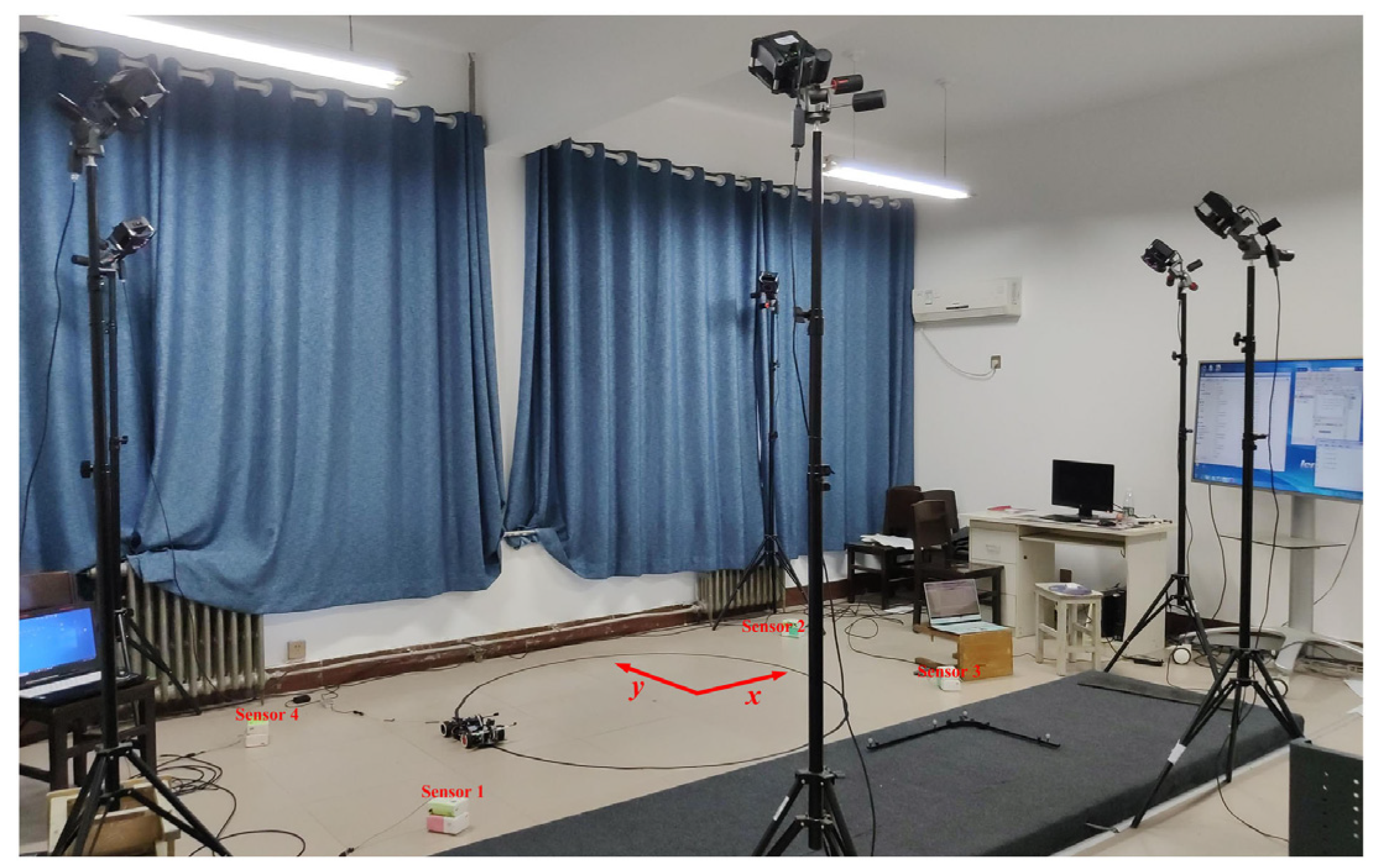
Consider the widely representative 2-D nearly-constant-velocity target tracking problem within a sensor network, which is commonly utilized in the literature [37] of distributed filtering, where the target’s positions are measured amidst clutter. The system model is described as

$$x_k=\left[\begin{array}{cccc}1& t& 0& 0\\ 0& 1& 0& 0\\ 0& 0& 1& t\\ 0& 0& 0& 1\end{array}\right]x_{k-1}+\left[\begin{array}{cc}\frac{t^2}{2}& 0\\ t& 0\\ 0& \frac{t^2}{2}\\ 0& t\end{array}\right]w_k,$$

(52)

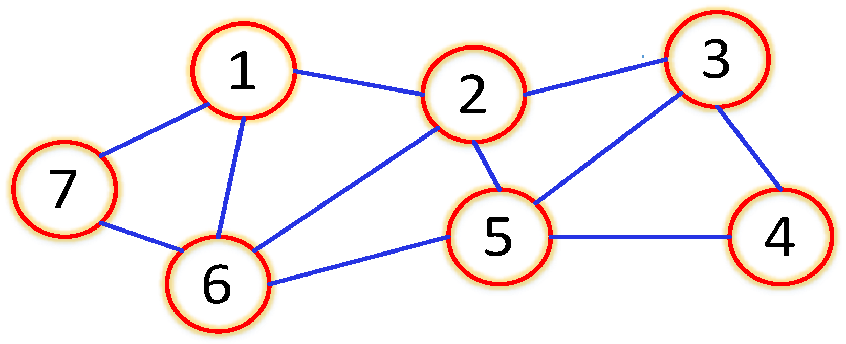
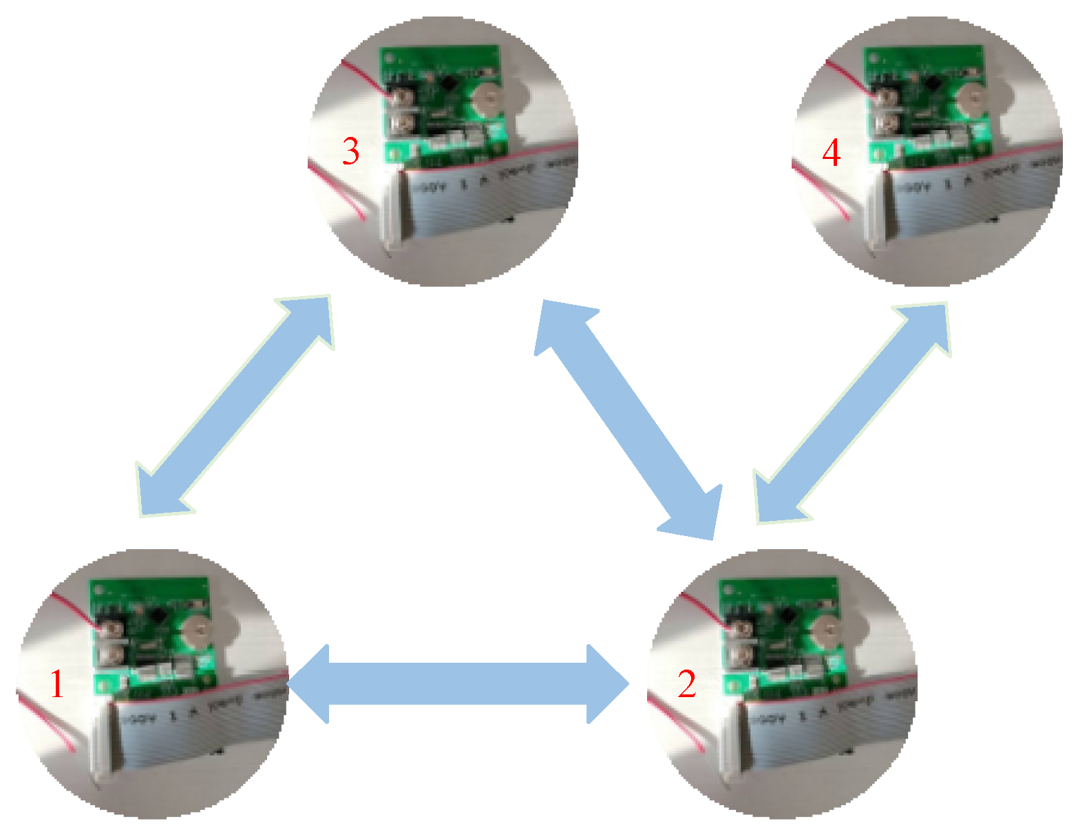
where $x_k={[\begin{array}{cccc}{x}_k& {\dot{x}}_k& y_k& {\dot{y}}_k\end{array}]}^T$, $(x_k,y_k)$ and $({\dot{x}}_k,{\dot{y}}_k)$ are respectively the position and velocity of tracking targe in x and y directions. The sampling period is selected as t = 1 s. There are seven sensors to observe the target, and the communication topology graph among sensors is shown in Figure 1.

In the linear model, the measurements are the positions of the target, and the corresponding measurement model is given by

$$z_k^s=\left[\begin{array}{cccc}1& 0& 0& 0\\ 0& 0& 1& 0\end{array}\right]x_k+{\upsilon }_k^s.$$

(53)

The initial value of the target is $x_0={\left[100,1,100,1\right]}^T$ with covariance $P_0=\mathrm{diag}\left(\left[100,5,100,5\right]\right)$. To guarantee the convergence of fixed-point iteration, the fixed-point iterative threshold and the maximum number of fixed-point iterations are preset as $\epsilon ={10}^{-6}$ and $N_{\max }=60$.

The root-mean-square error (RMSE) and the average (RMSE) are adopted as the performance evaluation benchmarks. The RMSE and ARMSE of the position are calculated as

$$\left\{\begin{array}{l}{\mathrm{RMSE}}_{\mathrm{pos}}(k)=\sqrt{{\displaystyle \frac{1}{M}}{\displaystyle \sum _{r=1}^M\left({(x_k^r-{\widehat{x}}_k^r)}^2+{\displaystyle \sum _{s=1}^S{(y_k^{s,r}-{\widehat{y}}_k^{s,r})}^2}\right)}},\\ {\mathrm{ARMSE}}_{\mathrm{pos}}={\displaystyle \frac{1}{K}}{\displaystyle \sum _{k=1}^K{\mathrm{RMSE}}_{\mathrm{pos}}(k)},\end{array}\right.$$

(54)

where M is the count of Monte Carlo runs, K is the total simulation period, and $({\widehat{x}}_{k,r}^s,{\widehat{y}}_{k,r}^s)$ is the estimation of the true position $(x_k^s,y_k^s)$ at the s-th sensor for the r-th Monte Carlo experiment. The RMSE and ARMSE of velocity are calculated to those for the above position. The total time steps K are chosen as K = 200 s and the total Monte Carlo runs are M, selected as M = 100. All the simulations are conducted in MATLAB 2016b and run on an Intel Core i7-7700HQ, 2.80 GHz, 8 GB PC.

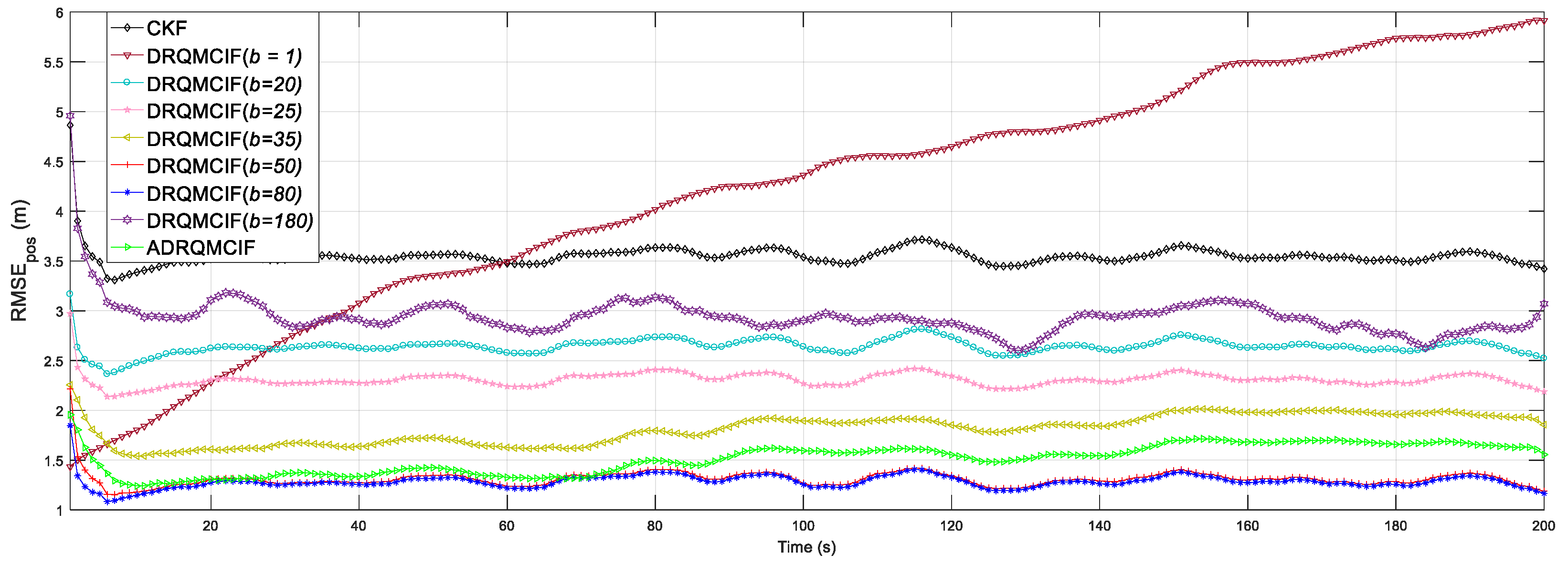
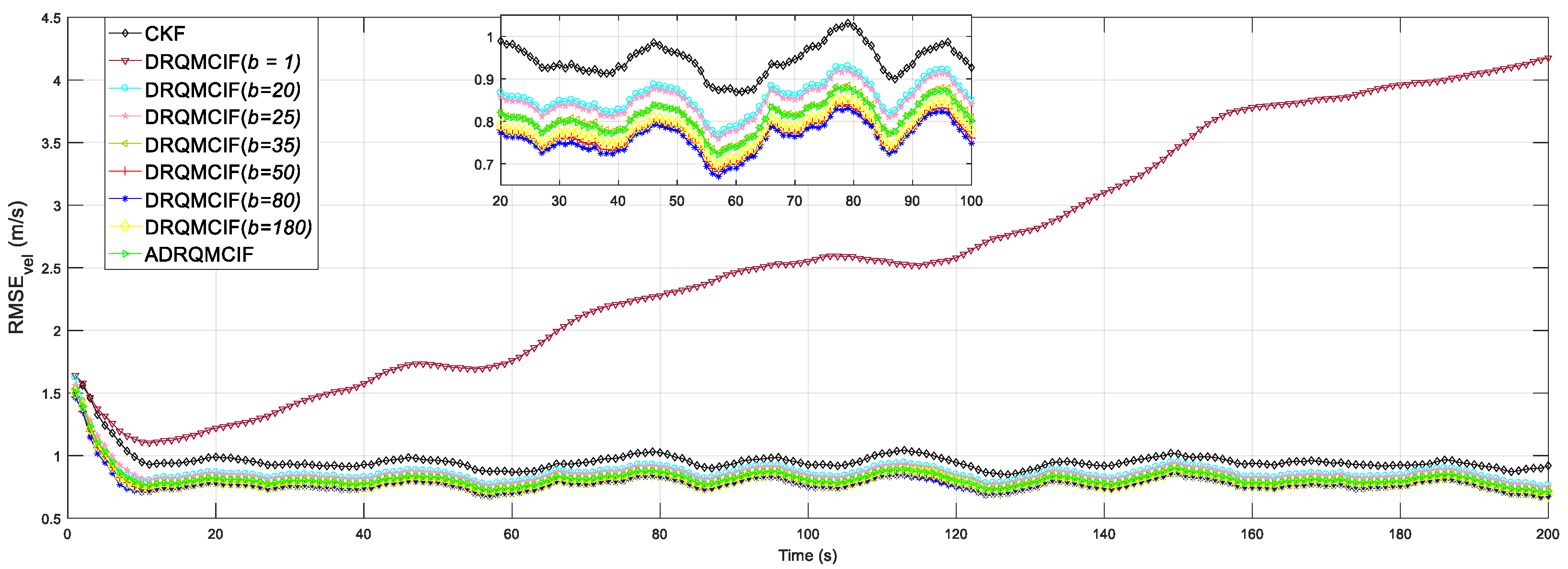
4.2. The Influence of Kernel Width

Firstly, the selection of the kernel width in the kernel function application can greatly influence the algorithm’s estimation precision and robustness. Therefore, the different kernel widths under the proposed DRQMCIF algorithm are discussed in this section.

This is considering that the process noise is Gaussian but the measurement noises are Gaussian mixture noise as follows

$${\mathbf{w}}_k\sim N\left(0,Q\right),$$

(55)

$${\mathbf{v}}_k\sim 0.9N\left(0,R\right)+0.1N\left(0,200R\right),$$

(56)

where 0.9 and 0.1 are the probabilities in Gaussian mixture noises separately, $Q=0.01I_2$ and $R=4I_2$. The Gaussian mixture noise is one of the representatives of non-Gaussian noise. The consensus iterative number L is set as L = 10. Let the kernel width c = 1, 20, 25, 35, 50, 80, 180, respectively. The confidence level factor is chosen by $\tau =3.5$, and the maximum kernel width is preset as b_max = 90 in the proposed adaptive kernel width. The measurement noises in Equation (56) are one of the typical heavy-tailed non-Gaussian noises with a mixed-Gaussian distribution, which is often employed in the non-Gaussian filtering literature [20,37].

From Figure 2 and Figure 3, a too-small kernel width may decrease the estimation accuracy and robustness performance of the proposed DRQMCIF algorithm; for example, the DRQMCIF algorithm is even divergent when the kernel width b = 1. As the kernel width grows, the ARMSEs under the DRQMCIF algorithm get smaller and smaller, which means that the estimation accuracy is getting higher and higher. However, a too-large kernel width would make the DRQMCIF estimation performance decrease severely. It can easily be seen that the DRQMCIF estimation accuracy with the kernel width b = 180 is lower than b = 80. With the increase in the kernel width, the effect of the DRQMCIF algorithm effect reduces to the CKF. Thus, the estimation performance is influenced magnificently by the selection of the kernel width. It is concluded that the optimal kernel width is b = 80 from Figure 2 and Figure 3. According to the simulation results, the kernel width amid [50, 80] can acquire better estimation precision for the proposed DRQMCKF algorithm. The DRQMCIF algorithm result under the adaptive kernel width cannot reach that under the suitable kernel width b ∈ [50, 80]. Therefore, when the optimal kernel width selects b = 80, the proposed DRQMCKF algorithm can acquire better estimation precision and robustness performance than that under other kernel widths and adaptive kernel widths.

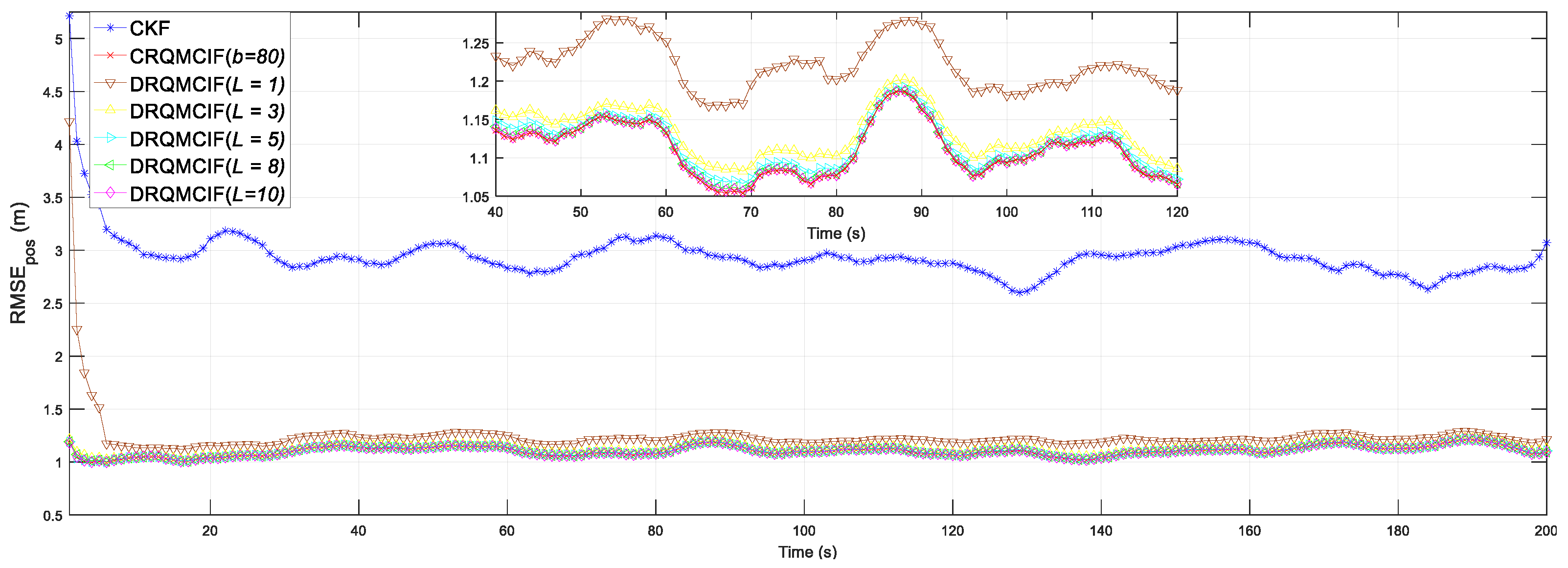
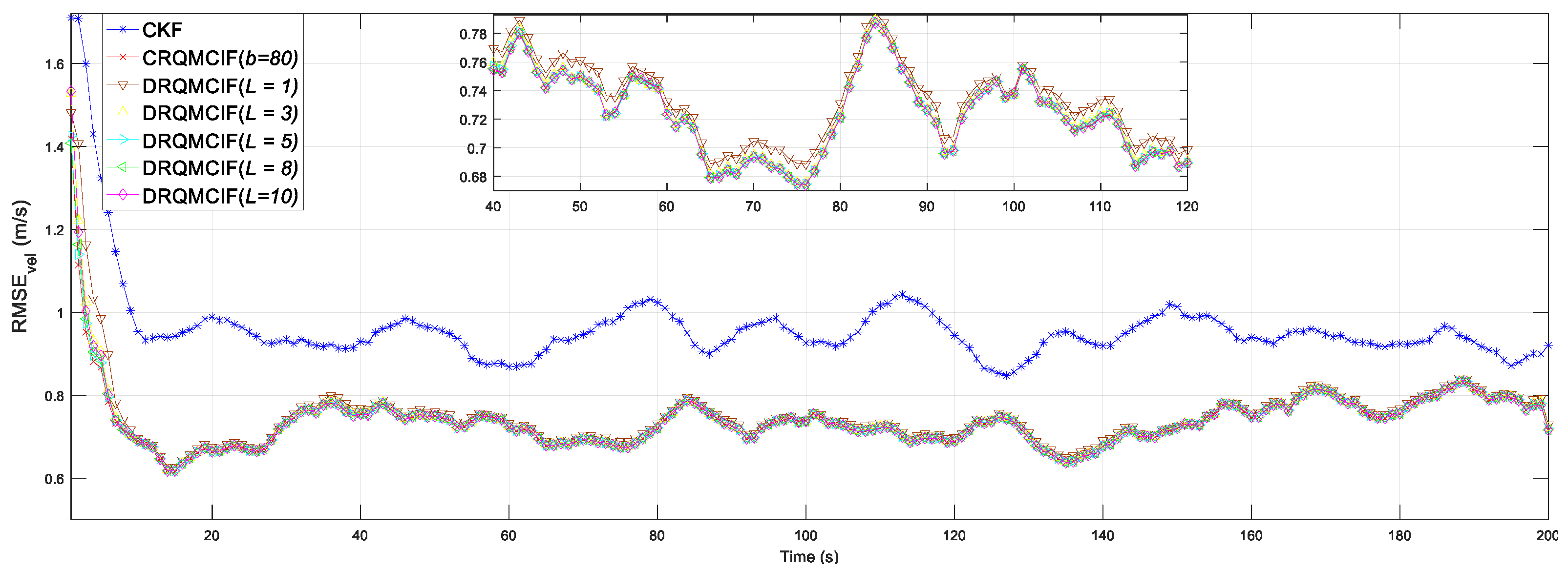
4.3. The Impact of Consensus Iterations

To assess the impact of consensus iterations, the devised DRQMCKF algorithm is simulated for the consensus iteration L = 1, 3, 5, 8, 10 under the same noise interference (in Equations (55) and (56)) as Section 4.2. The kernel width is selected as b = 80 from the conclusion in Section 4.2. The CRQMCIF and CKF algorithms are employed as the performance counterparts. Both CRQMCIF and DRQMCIF algorithms choose the optimal kernel width b = 80 obtained in Section 4.2.

The simulation outcomes are shown in Figure 4 and Figure 5. From these two figures, it can be seen that the estimation precision and performance would enhance when the consensus iteration number increases. The proposed DRQMCIF algorithm approximates the performance of the CRQMCIF algorithm when the number of consensus iterations L = 10, which illustrates that the consensus result of the distributed filtering algorithm will be closer to the global optimum (i.e., the central filtering algorithm) and can improve the accuracy of distributed filtering as the number of consensus iterations increases. When the number of consensus iteration L = 10, the performance of the proposed DRQMCIF algorithm is approximately equal to that of the CRQMCIF algorithm, which verifies the conclusion just mentioned. On the other side, the distributed algorithm could still acquire relatively better estimation performance under the consensus iteration number L = 5 and L = 8, which is of practical application for real sensor networks with limited communication resources. Each consensus iteration requires the exchange of information between nodes. If there are too many iterations, the communication requirements increase significantly, especially in large-scale networks, which may lead to bandwidth exhaustion or increased latency. Therefore, a smaller number of consensus iterations can be chosen in practical applications to avoid possible bandwidth exhaustion or delay increases, for instance, the number of consensus iterations can select L = 5, which may reach a better estimation performance in the practical engineering application.

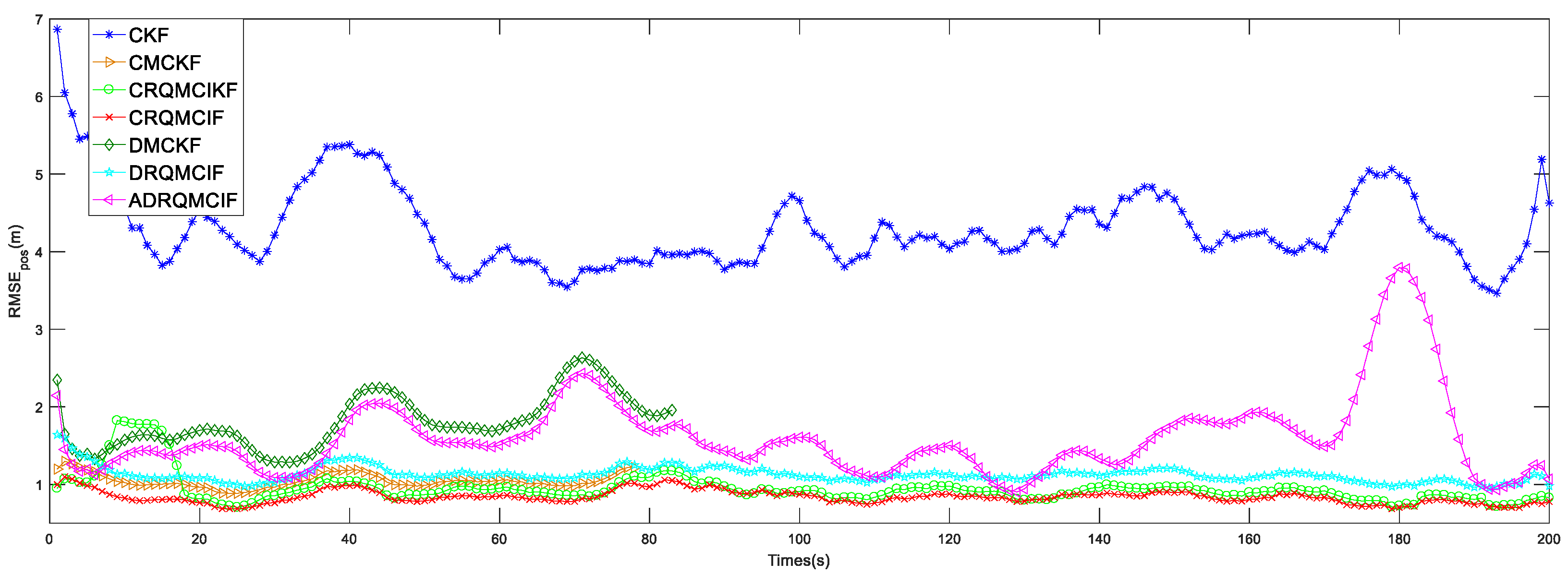
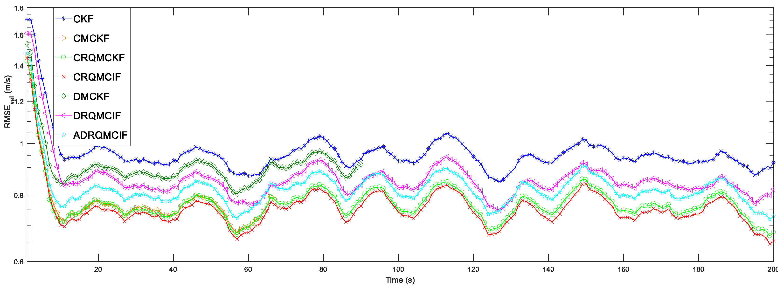
4.4. Comparisons with the Relevant Algorithms

In this subsection, the performance of the proposed algorithms is contrasted with other related filter algorithms under the non-Gaussian noise. The following several algorithms are evaluated: the CRQMCKF (Algorithm 1), the CRQMCIF (Algorithm 2), the DRQMCIF (Algorithm 3), the (ADRQMCIF) (Algorithm 4), the CKF, the centralized maximum correntropy Kalman filter (CMCKF) [20] and the distributed maximum correntropy Kalman filter (DMCKF) [37]. The three performance indexes are adopted in the following discussion, which are RMSEs and ARMSEs of the position and velocity defined in Section 4.1, and the single-step run time (SSRT), separately.

In the following simulation comparisons, the kernel width under the DRQMCIF algorithm is selected as b = 80 according to the discussion in Section 4.2 and the consensus iterations are chosen as L = 10 according to the discussion in Section 4.3. To ensure a fair evaluation, the kernel width of the existing CMCKF is set as σ = 2 because this configuration provides better estimation performance compared to σ = 80 under these specified simulation conditions according to the results in the reference article [20]. For the ADRQMCIF algorithm, the pre-setting maximum kernel width selects b_max = 90 according to the conclusion in Section 4.2, and the confidence level factor is chosen as $\tau$ = 3.5. The two scenarios where the process and measurement noises are set as Gaussian-mixture and t non-Gaussian noise, respectively.

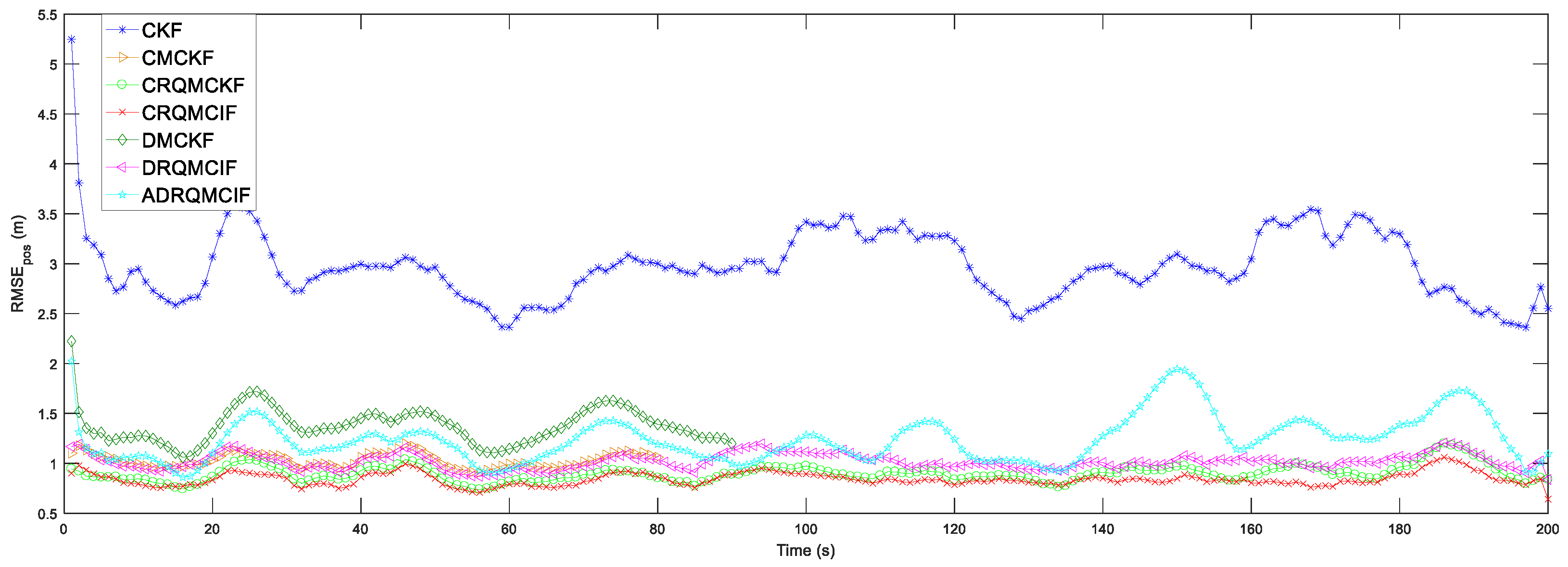
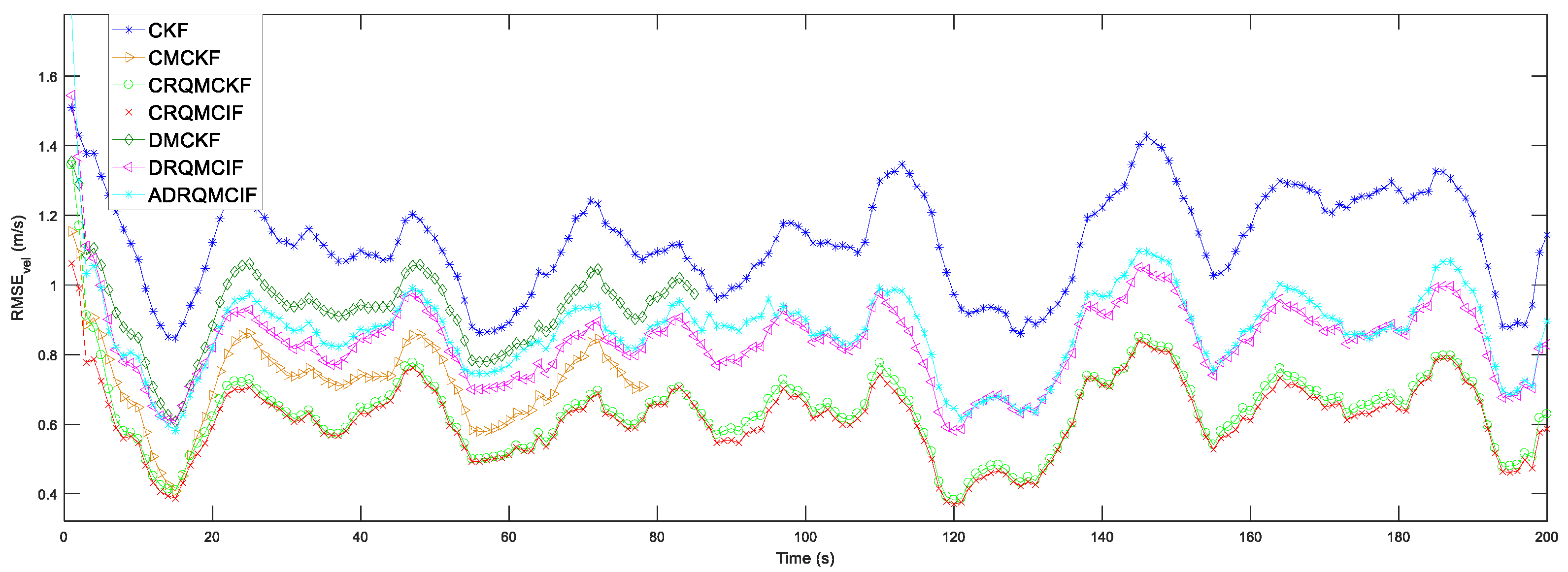
4.4.1. Scenario 1

In scenario 1, the process and measurement noises are assumed as the Gaussian-mixture noises, which is one of the representatives of common non-Gaussian noise,

$${\mathbf{w}}_k\sim 0.9N\left(0,Q\right)+0.1N\left(0,40Q\right),$$

(57)

$${\mathbf{v}}_k^s\sim 0.9N\left(0,R\right)+0.1N\left(0,200R\right),$$

(58)

where $Q$ and $R$ are the same as in Section 4.2.

The simulation outcomes under Gaussian-mixture noise are displayed in Figure 6 and Figure 7 and

Table 2. ARMSEs of different algorithms under Scenario 1 (Gaussian-mixture noise).

Algorithms	ARMSEpos (m)	ARMSEvel (m/s)	SSRT (s)
CKF	12.3577	2.7098	0.0913
CMCKF	4.7308	2.0316	0.9275
CRQMCKF	4.1075	1.9351	0.7687
CRQMCIF	4.1070	1.9342	0.8182
DMCKF	4.8356	2.1823	2.8724
DRQMCIF	4.7421	2.1276	2.0586
ADRQMCIF	5.2327	3.4897	4.7827

. The estimation capability of the CKF algorithm is the worst among all algorithms due to the breakdown of the Gaussian noise assumption since the CKF algorithm is suitable to be employed in Gaussian noise problems. The RMSEs and ARMSEs of the position and velocity in these CMCKF, CRQMCKF, CRQMCIF, DRQMCIF, and ADRQMCIF algorithms are less than that of the CKF algorithm for all these algorithms and are based on MCC, which is specialized in handling the non-Gaussian noise problems. From Table 2, compared with the CMCKF algorithm, the proposed CRQMCIF algorithm improves the ARMS_pos by 13.18%, the ARMSE_vel by 4.75%, and the single-step run time (SSRT) by 13.89%; the proposed CRQMCKF algorithm improves the ARMS_pos by 13.18%, the ARMSE_vel by 4.75%, and the single-step run time (SSRT) by 17.12%. These outcomes illustrate that the estimation precision of the CRQMCIF algorithm is equivalent to that of the CRQMCKF algorithm and the single-step run time of the CRQMCIF is higher than that of the CRQMCKF algorithm since the information matrices increase the computational burden. Compared to the DMCKF algorithm, the proposed DRQMCIF in this paper improves the ARMS_pos by 1.93‰, the ARMSE_vel by 2.51%, and the single-step run time (SSRT) by 28.33%. However, the ARMS_pos, the ARMSE_vel, and the single-step run time (SSRT) of the ADRQMCIF algorithm are degraded because adaptive filtering recalculates the kernel width at each step based on error, which does not achieve the performance of the DRQMCIF under the optimal kernel width and leads to an increase in the computation time.

From Figure 6 and Figure 7, it can be seen that the proposed CRQMCKF, CRQMCIF, DRQMCIF, and ADRQMCIF algorithms based the rational quadratic kernel function can run to the specified step length and end prematurely compared to the CMCKF and DMCKF algorithms based the Gaussian kernel function. The CMCKF and DMCKF algorithms are unable to reach the required step and end the algorithm prematurely because the Gaussian kernel function induces a singular matrix. Compared with the Gaussian kernel function, the rational quadratic kernel function offers several advantages: it is robust to outliers and non-Gaussian noise; it can avoid the appearance of the singular matrices; it has lower computational complexity for that rational quadratic kernel function and avoids the exponential operation and thus reduces a large amount computational burden. These several benefits make the rational quadratic kernel function more suitable for data characterized by non-Gaussian heavy-tailed noise or large outliers. In contrast, the Gaussian kernel function is more sensitive to outliers and has a higher computational expense. However, the estimation performance of the ADRQMCIF algorithm cannot reach that of the DRQMCIF algorithm with the optimal kernel width. When the optimal kernel width cannot be determined in the practical engineering application, the ADRQMCIF algorithm can be an alternative algorithm to deal with the distributed state estimation problem under non-Gaussian noise interference.

4.4.2. Scenario 2

In scenario 2, the process and measurement noises are assumed to obey t distribution with the degree of freedom 1,

$${\mathbf{w}}_k\sim t(1),{\mathbf{v}}_k^s\sim t(1).$$

(59)

t distribution is one of the probability distributions that is similar to the normal distribution with its bell shape but has heavier tails and is one of the non-Gaussian noises. The probability distribution function of the d₁-dimension t distribution is

$$f(x)=\left[\mathrm{\Gamma }\left((\nu +d_1)/2\right)\right]/\left[\sqrt{{(\nu \pi )}^{d_1}|\Sigma |}\cdot \mathrm{\Gamma }\left(\nu /2\right)\right]\cdot {\left(1+{\displaystyle \frac{1}{\nu }}{\left(x-\mu \right)}^{\mathrm{T}}{\Sigma }^{-1}(x-\mu )\right)}^{-{\displaystyle \frac{\nu +d_1}{2}}},$$

where $x\in {ℝ}^{d_1}$, $\mu \in {ℝ}^{d_1}$ is the mean vector, $\Sigma \in {ℝ}^{d_1\times d_1}$ denotes the covariance matrix or scale matrix satisfying $\Sigma =((v-d_1)/v)E[(x-\mu ){\left(x-\mu \right)}^{\mathrm{T}}]$, $\nu$ is the freedom, $\mathrm{\Gamma }(\cdot )$ is gamma function, and $\mathrm{\Gamma }(s)={\displaystyle {\int }_0^{+\infty }{\mathrm{e}}^{-x}{x}^{s-1}\mathrm{d}x}$.

The simulation results under t noise (which is another non-Gaussian noise) are exhibited in

Table 3. ARMSEs of different algorithms under Scenario 2 (t noise).

Algorithms	ARMSEpos (m)	ARMSEvel (m/s)	SSRT (s)
CKF	13.2687	2.9153	0.1056
CMCKF	4.7308	2.1546	0.9738
CRQMCKF	4.2145	2.0372	0.8367
CRQMCIF	4.1352	2.0354	0.8416
DMCKF	4.9035	2.2357	2.9015
DRQMCIF	4.8216	2.1428	2.1306
ADRQMCIF	5.3596	3.5341	4.8105

and Figure 8 and Figure 9. Since t noise destroys the assumption of Gaussian noise, which is a prerequisite for the good estimation performance of the CKF algorithm, the estimation performance of the CKF algorithm is significantly worse than the other algorithms. From Table 3, compared to the CMCKF algorithm, which is based on the Gaussian kernel function, the proposed CRQMCKF increases the ARMS_pos by 10.91%, the ARMSE_vel by 5.45%, and the single-step run time (SSRT) by 14.08%; the proposed CRQMCIF algorithm improves the ARMS_pos by 12.59%, the ARMSE_vel by 4.16%, and the single-step run time (SSRT) by 8.88%. These results show that the estimation accuracy of the CRQMCKF algorithm approximates that of the CRQMCIF algorithm and the single-step run time of the CRQMCIF is larger than that of CRQMCKF algorithm because the information matrix enhanced the computation burden of the CRQMCIF algorithm. Compared to the DMCKF algorithm, the proposed DRQMCIF in this paper improves the ARMS_pos by 1.67‰, the ARMSE_vel by 2.51%, and the single-step run time (SSRT) by 26.57%, whereas the ARMS_pos, the ARMSE_vel, and the single-step run time (SSRT) of the ADRQMCIF algorithm are higher than that of the DMCKF algorithm since adaptive filtering needs to repeatedly calculate the corresponding kernel width according to the different error values at each step, which cannot reach the estimation performance of the DRQMCIF with the optimal kernel width and meanwhile results in an increase in the SSRT computation time.

From Figure 8 and Figure 9, it can easily be concluded that the presented CRQMCKF, CRQMCIF, DRQMCIF, and ADRQMCIF algorithms can arrive at the assigned step length; however, the CMCKF and DMCKF algorithms based on Gaussian kernel function were forced to end early. When the Gaussian function encounters a large outlier, its function rapidly becomes smaller or even tends to 0. When its function value exceeds the calculation accuracy of the computer, a singular matrix will appear and the algorithm will be forced to end early. The rational quadratic kernel function can easily avoid this situation. Simultaneously, the rational quadratic kernel function is only operated by addition, subtraction, multiplication, and division, so the exponential operation is avoided, and the computational complexity of the related algorithms will be reduced. Finally, the estimation accuracy of the ADRQMCIF algorithm cannot acquire that of the DRQMCIF algorithm with the optimal kernel width. When the optimal kernel width cannot be obtained in the engineering application, the ADRQMCIF algorithm can be chosen to resolve the distributed state estimation problems interfered with by the large outlier non-Gaussian noise.

In sum, from the discussion of two different non-Gaussian noises, Scenario 1 and Scenario 2, it can be seen that the distributed maximum correntropy linear algorithms based on rational quadratic kernel function are superior to the corresponding algorithms based on the Gaussian kernel function.

5. Experimental Setup for Multi-Sensor Target Tracking

5.1. Experimental Setup and Parameter Settings

To assess the practical performance of the proposed estimator, a multi-sensor experimental platform was constructed for the task of dynamic target tracking, as illustrated in Figure 10. The platform consists of a test vehicle equipped with an electromagnetic drive, a Nokov motion capture system with six Mars 2 cameras, 24 GHz millimeter-wave radar sensors, and multiple PCs for data acquisition and processing, and so on. The motion capture system provides sub-millimeter accuracy and serves as the ground-truth reference for the target’s position.

The camera system has a detection range of 0~1 m with a precision of 0.3 mm, while the radar sensors operate over a range of 0.1~3.5 m with a resolution of approximately 50 mm. The distributed sensor network is constructed using multiple CP210x USB-to-UART modules, where each sensor node communicates with the central processor. The test vehicle moves in a circular trajectory driven by magnetic propulsion and is used as the maneuvering target throughout the experiment. The vehicle model refers to the setup described in [40].

The communication topology of the sensor network is shown in Figure 11, comprising four sensor nodes $S=\{1,2,3,4\}$, and the directed edges are defined by

ε = {(1,1),(1,2),(1,3),(2,1),(2,2),(2,3),(2,4),(3,1),(3,2),(3,3),(4,2),(4,4)}.

This network enables decentralized estimation in a distributed framework, following the model structure referenced in [41].

The physical coordinates of the sensor nodes are fixed at the following:

• Sensor 1: (−141.891 cm, 72.019 cm),
• Sensor 2: (149.451 cm, 58.072 cm),
• Sensor 3: (128.305 cm, −72.313 cm),
• Sensor 4: (−165.279 cm, 56.663 cm).

In the simulation, both process and measurement noises are considered as Gaussian with zero mean and bounded variances. The process noise upper bound is set as Q_k= diag([0, 0, 0, 0, 4 × 10⁻⁶]), and the measurement noise upper bound is ${\mathbf{R}}_k^s$ = 144. Due to asynchronous sensor updates, the system experiences random time delays, with a maximum delay set to d = 6.

The estimator parameters are configured as follows:

• τ₁ = 1.1, τ₂ = 5, τ₃ = 0.01,
• λ₀ = 0.7, λ_m = 0.01 for m = 1, …, 5 and λ₆ = 0.99.
• The initial state covariance is P₀^s = diag([5, 5, 10, 2, 0.003]).

The test vehicle begins from position (0 cm, −94 cm), and after a 3 s initialization, follows a circular path at an initial speed of 98 cm/s, with an average velocity of approximately 75 cm/s under a uniform magnetic field. The sensor sampling period is 100 ms.

5.2. Evaluation and Comparison

Figure 12 presents the position estimation errors of the proposed method compared with the benchmark algorithms described in [42,43]. Notably, because the test vehicle is a physical object with non-negligible dimensions, measurement deviations arise not only from internal sensor noise but also from occlusion, reflection, and the spatial extent of the vehicle body itself, which cannot be idealized as a point mass, and the sensor readings are subject to both intrinsic sensor noise and external disturbances caused by the car’s body. Moreover, from the analysis of sensor output, intermittent measurement losses were observed for sensors 1 and 4 at various time instants during the experiment.

For the estimator reported in [42], the error intervals are recorded as ranging from [−28.16 cm, 24.14 cm] and [−27.27 cm, 22.33 cm], with corresponding mid-values of 10.32 cm and 3.34 cm. In contrast, the distributed estimation approach in [43] yields the range of [−17.16 cm, 13.97 cm] and [−7.87 cm, 23.78 cm], with mid-values of 3.83 cm and 6.03 cm, respectively. For the single-sensor DRQMCIF method (sensor 1), the position errors are found within [−17.38 cm, 30.96 cm] and [−7.05 cm, 23.77 cm], with mid-values of 6.54 cm and 4.31 cm.

According to the results illustrated in the figure, the DRQMCIF algorithm based on a single sensor does not exhibit satisfactory performance, indicating that its estimation accuracy is limited in the absence of multi-sensor collaboration. When extended to a multi-sensor framework, the proposed estimator achieves error med-values of approximately 1.84 cm and 1.14 cm, with value ranges of [−8.09 cm, 23.18 cm] and [−8.93 cm, 13.16 cm], highlighting a notable advantage in both accuracy and robustness over the benchmark estimators in [42] and [43].

The collective results from simulations, experiments, and comparisons clearly affirm the superiority of the proposed DRQMCIF approach in terms of both robustness and accuracy under the non-Gaussian noise interference in the multi-sensors network. Future investigations will focus on incorporating other non-Gaussian noise models to further enhance estimation performance.

6. Conclusions

In this paper, some centralized and distributed maximum correntropy linear filters based on a rational quadratic kernel function are devised for state estimation over the sensor network system under the non-Gaussian noise, where each sensor transmits solely to its neighboring sensors without the need for a fusion center. A classical target tracking numerical simulation over the sensor network displays the performance and robustness of the proposed filter algorithms based on the appearance of the non-Gaussian noise interference. The proposed distributed algorithms can achieve a balance between the estimation precision and exchange burden when the optimal kernel width b = 80 is obtained. Although the optimal consensus performance is achieved when the number of iterations is selected to L = 10, the case of L = 5 still provides satisfactory estimation results in practical scenarios. Importantly, reducing the number of iterations to L = 5 leads to a notable decrease in the computational load. As such, adopting L = 5 represents a practical compromise that maintains acceptable estimation accuracy while significantly improving the computational efficiency. Further, when the optimal kernel width cannot be predetermined, the adaptive kernel distributed filter is a kind of substitute algorithm that can approximate the estimation performance in the practical application. However, several problems need to be further researched in future work as follows: the distributed maximum correntropy algorithms based on a rational quadratic kernel function can be extended to a nonlinear sensor network system operation under non-Gaussian noise interference. The authors are required to learn more methods that can also be against non-Gaussian noise interference to be used as comparison algorithms. Additionally, to improve the practical engineering application value, it should address more cost-effective sensor network-evoked scenarios, for example, packet loss, data delay, and a time-varying topology network (i.e., dynamic sensor network).