On the Symmetry and Domination Integrity of Some Bidegreed Graphs

Abstract

Graphs are one of the dynamic tools used to solve network-related problems and real-time application models. The stability of the network plays a crucial role in ensuring uninterrupted data flow. A network becomes vulnerable when a node or a link becomes non-functional. To maintain a stable network connection, it is essential for the nodes to be able to interact with each other. The vulnerability of a network can be defined as the level of resistance it exhibits following the failure of communication links. Graphs serve as vital tools for depicting molecular structures, where atoms are shown as vertices and bonds as edges. The domination number quantifies the least number of atoms (vertices) required to dominate the entire molecular framework. Domination integrity reflects the impact of removing specific atoms on the overall molecular structure. This concept is valuable for forecasting fragmentation and decomposition pathways. In contrast to the domination number, domination integrity evaluates the extent to which the molecule remains intact following the removal of reactive or controlling atoms. It aids in assessing stability, particularly in the contexts of drug design, polymer analysis, or catalytic systems. This work focuses on the vulnerability parameter, specifically examining the domination integrity of a specific group of bidegreed hexagonal chemical network systems such as pyrene $PY\left(p\right)$, prolate rectangle $R_{p,q}$, honeycomb $HC\left(p\right)$, and hexabenzocoronene $HBC\left(p\right)$. This work also extends to the calculation of the domination integrity value for Cyclic Silicate $C{C}_p$ and Chain Silicate $C{S}_p$ chemical structure networks.

1. Introduction

Graph theory is fundamental in mathematical chemistry, facilitating the modeling of diverse chemical reactions. Molecular graphs illustrate the arrangement of covalently bonded compounds by employing vertices to denote atoms and edges to signify bonds. These graphical representations offer valuable insights into molecular structure and assist in the examination of diverse chemical properties. To identify specific categories of chemical compounds, graph enumeration techniques are employed, which are vital for computerized chemical identification and offer various strategies for enumeration. In biochemistry, it is critical to omit certain atom samples to address conflicts that may arise when comparing two chemical compounds. Numerous investigations within the domains of Quantitative Structure–Activity Relationship (QSAR) and Quantitative Structure–Property Relationship (QSPR) have underscored a robust and consistent association between the physical and chemical characteristics of molecules and specific graph-theoretical metrics referred to as topological indices or molecular descriptors. Among the diverse topological indices, the domination number has surfaced as particularly significant. This parameter, grounded in graph theory, quantifies the minimum number of vertices necessary to guarantee that every other vertex in the graph is either part of this set or directly adjacent to a vertex within the set. The domination integrity has demonstrated its utility as a valuable predictor of molecular behavior, stability, and reactivity, thereby playing a crucial role in the formulation of predictive models in the fields of chemistry and drug design. Domination theory is essential for encoding binary strings into DNA sequences. Encryption techniques, including the basic and insertion methods, leverage graph domination to encrypt any chemical formula. In this process, each chemical formula is initially transformed into a binary string, which is subsequently encrypted using DNA steganography.

Consider a simple graph $\Omega =(\mathcal{V},\mathcal{E})$, where $\mathcal{V}$ represents the set of nodes and $\mathcal{E}$ represents the edges of $\Omega$. The order of $\Omega$, denoted as $p=\left|\mathcal{V}\right(\Omega \left)\right|$, is defined as the cardinality or number of elements in $\mathcal{V}$. The set of all nodes that are adjacent to a node $\vartheta$ in the graph $\Omega$ is referred to as the open neighborhood $N\left(\vartheta \right)$ of $\vartheta$, denoted as $N\left(\vartheta \right)=\{\zeta \in \mathcal{V}(\Omega )/\zeta$ is adjacent to $\vartheta \}$. The closed neighborhood $N\left[\vartheta \right]$ of $\vartheta \in V\left(\Omega \right)$ is given by $N\left[\vartheta \right]=N\left(\vartheta \right)\cup \left\{\vartheta \right\}$. The degree of a vertex $\vartheta \in \mathcal{V}(\Omega )$ is determined by the number of edges incident with it, and it is represented as $deg\left(\vartheta \right)$. The geodesic distance, denoted as $d(\vartheta ,\zeta )$, refers to the shortest distance between two nodes $\vartheta$ and $\zeta$. An independent set K of vertices is characterized as a subset of $\mathcal{V}$ where no two vertices within K are adjacent. The independent number $\beta (\Omega )$ represents the largest quantity of elements found in a maximal independent set of $\Omega$. The notion of dominating sets can be utilized to tackle various practical issues encountered in the real world. The principle of domination has been applied in a variety of real-time problem contexts, such as networks, communication monitoring, and more. Let K denote a subset of $\mathcal{V}(\Omega )$. If each vertex in $\mathcal{V}-K$ is linked to at least one vertex in K, then K is termed a dominating set. The minimum size of a dominating set is represented by the domination number $\gamma (\Omega )$.

In 1990, a comprehensive analysis of this parameter was presented by Hedetniemi and Laskar [1]. The notions of strong and weak domination in the realm of graph theory were first introduced and formally articulated by Pushpa Latha and Sampathkumar in their 1996 publication [2]. This introduction established a basis for differentiating various forms of domination within graphs, offering fresh insights and methodologies for examining the interactions and control dynamics among vertices in a network. In a subsequent study, Quadras et al. examined the bondage number and domination number for three particular structures: the Balaban 10-cage, the pyrene torus, and hexabenzocoronene [3]. Simultaneously, Mojdeh et al. examined the total and connected domination number for particular specific families of chemical graphs [4]. Suganya and Anitha focused their study on the independent domination number within cyclic and chain silicate structure [5]. Chithra et al. explored the notion of secure domination in honeycomb structures [6]. Shukura et al. [7] explored the concepts of resolvent energy and pseudospectrum energy in fullerene structures. Ante Graovac et al. [8] conducted a case study focusing on fullerene stability using a topological efficiency approach. Additionally, Shukura et al. [9] analyzed the behavior of orbits and their associated energy in weighted graphs. Almalki and Kaemawichanurat researched the domination number and independent domination number in hexagonal systems [10]. Finally, the relationship between the strength of graphs and their domination number was scrutinized by Takahashi et al. [11].

1.1. Scientific Motivation

The exploration of vulnerabilities in chemical graphs is driven by the objective of enhancing scientific knowledge, refining technological approaches, and tackling real-world issues across multiple fields, such as medicine, materials science, and environmental science. The domination number measures the minimum quantity of atoms (vertices) necessary to dominate the complete molecular structure. The motivation stems from the observation that the domination number can be overly sensitive to local structural weaknesses and may not accurately reflect the overall vulnerability of a network. For instance, both the star graph $K_{1,n-1}$ and the graph $K_1+(K_1\cup K_{n-2})$ (where + denotes the join and ∪ denotes the disjoint union) have a domination number of one. However, they differ significantly in terms of network resilience. In $K_{1,n-1}$, the removal of the dominating set completely disrupts communication, while in $K_1+(K_1\cup K_{n-2})$, all but two stations remain connected. This demonstrates that the domination number alone is inadequate for assessing network vulnerability. In contrast, the domination integrity value of $K_{1,n-1}$ is 2, whereas for $K_1+(K_1\cup K_{n-2})$, it is $n-1$. These values indicate that $K_1+(K_1\cup K_{n-2})$ represents a more robust network structure than the star graph $K_{1,n-1}$. Therefore domination integrity reflects the impact of removing specific atoms on the overall molecular structure. This concept is valuable for forecasting fragmentation and decomposition pathways. In contrast to the domination number, domination integrity evaluates the extent to which the molecule remains intact following the removal of reactive or controlling atoms. It aids in assessing stability, particularly in the contexts of drug design, polymer analysis, or catalytic systems. Within quantitative structure–activity/property relationships, domination integrity may serve as a more effective descriptor for chemical activity, as it incorporates both control points and structural cohesion. To evaluate vulnerability, several theoretical parameters of graphs have been defined, such as toughness, degree of rupture, integrity, and connectivity.

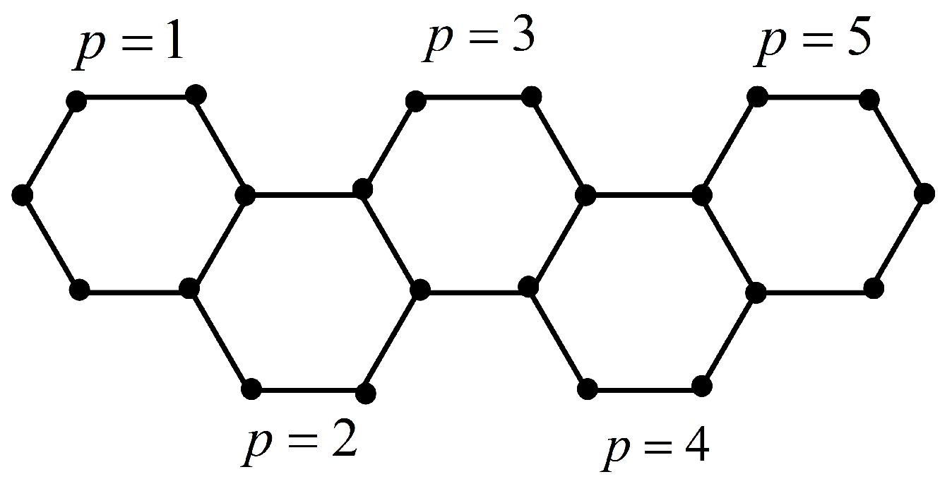
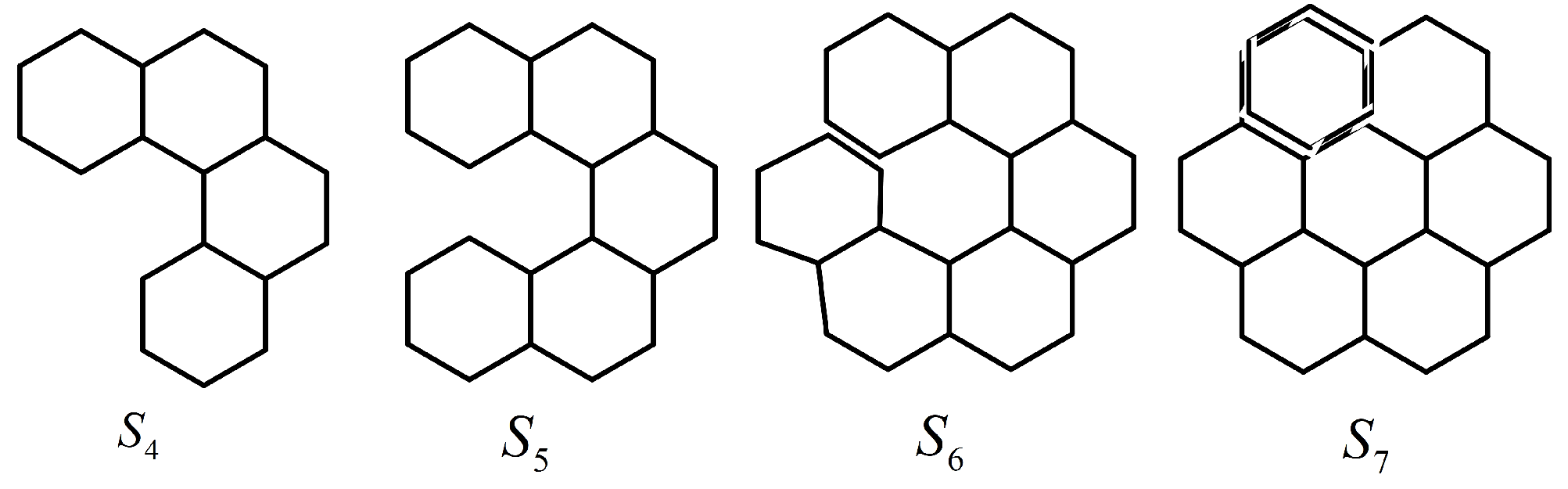
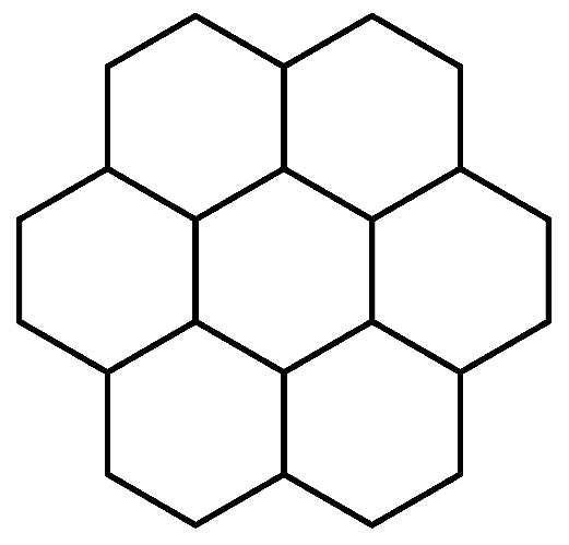
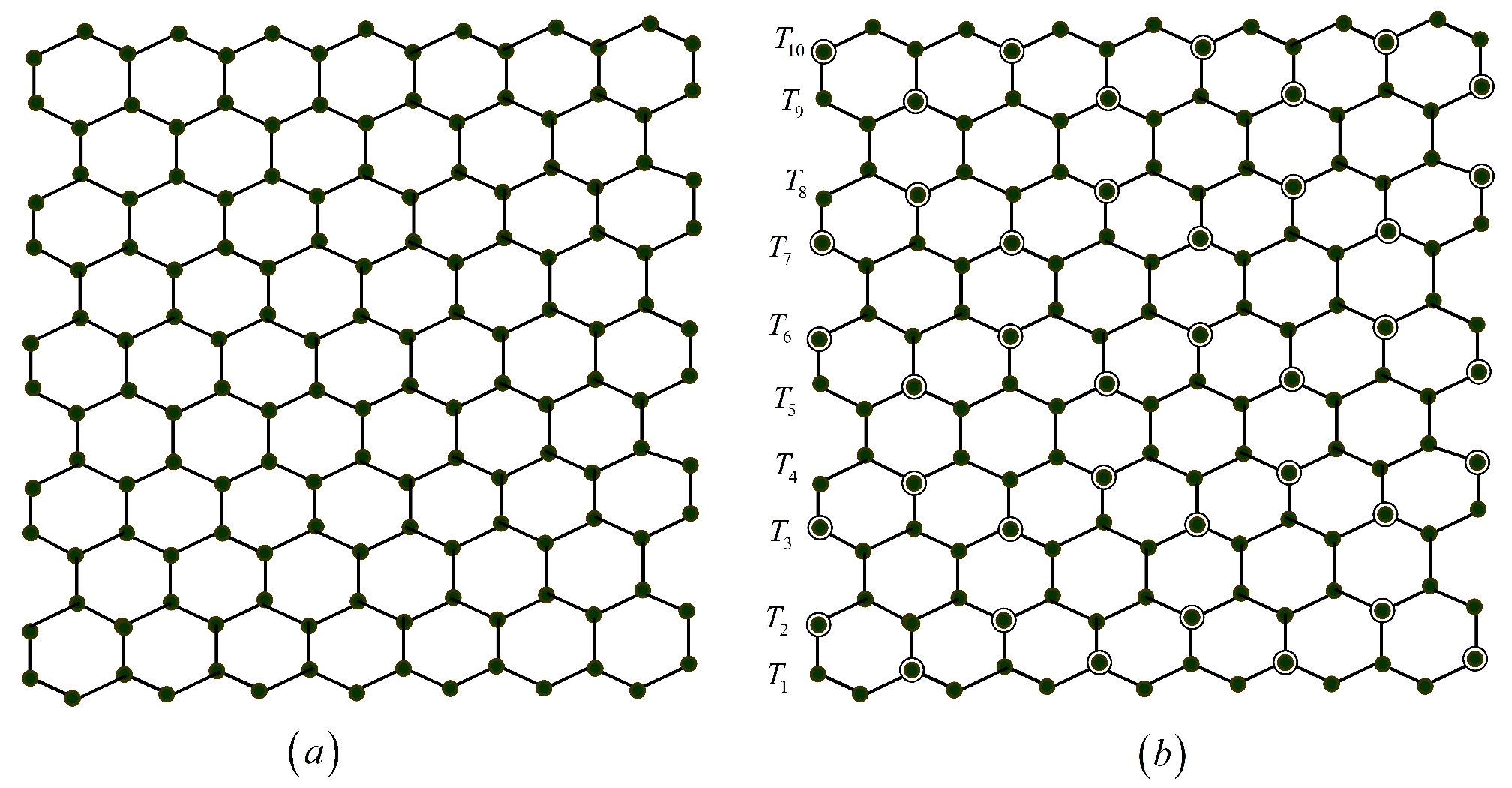
1.2. Hexagonal Systems

Hexagonal structures are defined as finite, interconnected planar networks made up entirely of regular hexagons, possessing the essential characteristic that the removal of any single vertex results in the disconnection of the network. In these structures, all internal areas are constituted by congruent regular hexagons. Two hexagons that share a common edge are regarded as adjacent. Each vertex, or node, in the hexagonal network has a degree of either two or three, indicating the number of edges incident to it. An internal vertex is defined as one located inside the structure rather than on its outer boundary. Hexagonal systems are of significant importance in theoretical chemistry because they naturally model benzenoid hydrocarbons through graph representations. A hexagonal chain is a specific type of hexagonal system where each vertex is incident to at most three hexagons, and no single hexagon shares edges with more than two adjacent hexagons. Hexagonal systems without internal vertices are classified as catacondensed, while those containing internal vertices are called pericondensed. In catacondensed systems, each hexagon can be adjacent to no more than three others, whereas in pericondensed systems, a hexagon may be adjacent to up to six others. Within a hexagonal chain consisting of p hexagons (with $p>2$), there are two terminal hexagons at the ends and $p-2$ hexagons in the middle, each connected to exactly two adjacent hexagons. A linear benzenoid graph containing p hexagons, referred to as a hexagonal chain C, is defined by the sequential arrangement of its hexagons [10]. Figure 1 shows $L\left(5\right)$, a hexagonal chain made up of five hexagons. When the hexagonal chain C alternates consistently between left $\left(L\right)$ and right $\left(R\right)$ turns, it is classified as a zigzag hexagonal system [3]. An example of such a zigzag hexagonal system with $p=5$ is shown in Figure 2. Furthermore, a spiral chain of dimension p, as illustrated in Figure 3, is observed in a hexagonal structure $S_p$ [5], which comprises a total of $4p+2$ vertices.

Honeycomb networks are crucial in the realm of chemistry, especially for modeling benzenoid hydrocarbons. Additionally, these networks are widely utilized across various fields, including computer graphics, cellular network base stations, and image processing. The honeycomb structure grid, referred to as $HC\left(p\right)$, is constructed by augmenting $HC(p-1)$ with an additional layer of hexagons along its boundary. In this context, p represents the quantity of hexagons located between the boundary and the center of $HC\left(p\right)$. Notably, $HC\left(p\right)$ comprises $6p^2$ vertices and $9p^2-3p$ edges. An example of a honeycomb network with a dimension of 2 is shown in Figure 4.

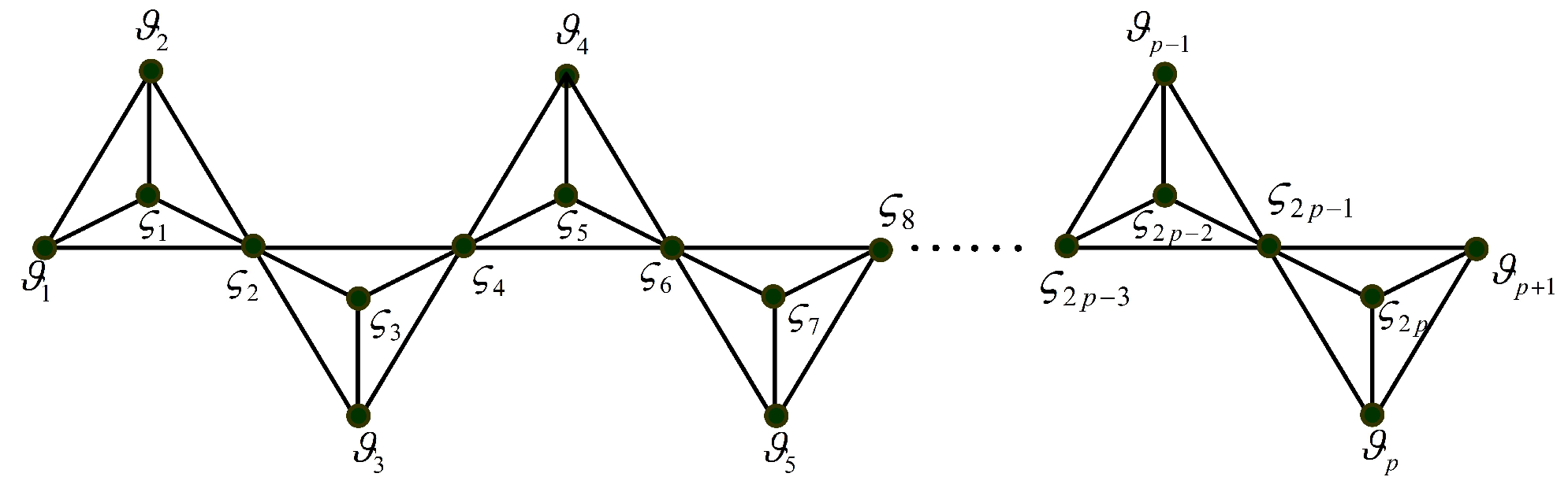
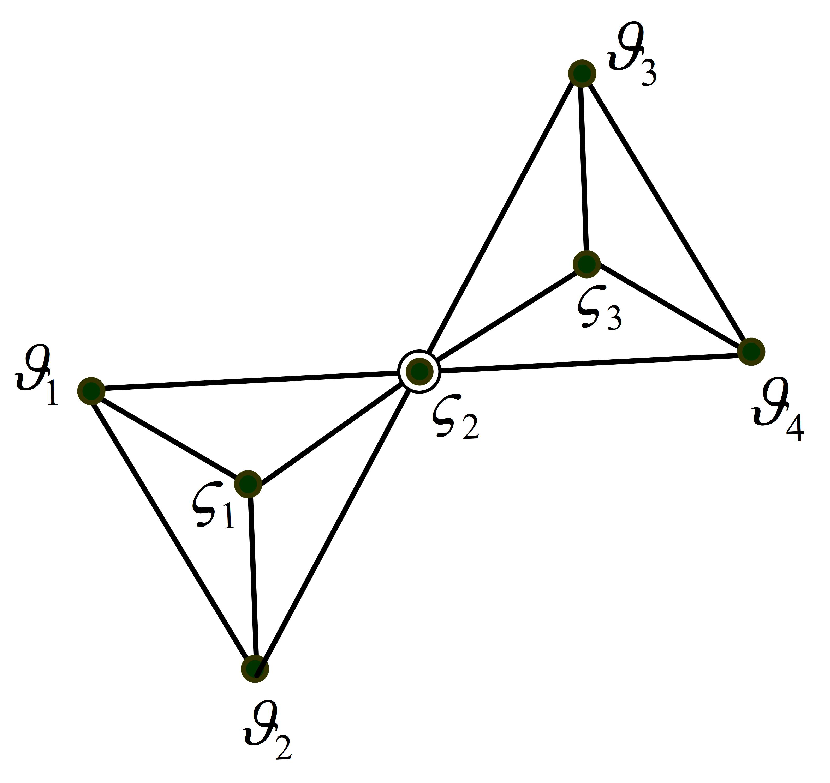
1.3. Silicate Networks

Silicates are created through the combination of sand with metal oxides or metal carbonates. These compounds are characterized by the presence of SiO₄ tetrahedra, which are found in nearly all silicates [12]. In the context of chemistry, the oxygen ions are depicted at the corner vertices of the SiO₄ tetrahedron, while the central vertex signifies the silicon ions. The corner vertices are referred to as oxygen nodes, whereas the central vertex is known as a silicon node. The formation of minerals occurs via the linkage of oxygen nodes from two distinct silicate tetrahedra in a particular sequence. The configuration of these tetrahedra is crucial in defining the various types of silicate structures. Figure 5 illustrates several structural units found in silicates. The formation of a chain silicate network structure, referred to as $C{S}_p$, with a dimension of p, is accomplished by aligning p tetrahedra in a sequential arrangement [12]. This specific structure is defined by possessing $3p+1$ vertices and $6p$ edges. The 6-dimensional chain silicate network $C{S}_6$ is depicted in Figure 6. A cyclic network structure, referred to as $C{C}_p$ for $p\ge 3$, is created by interlinking p tetrahedra. This network, characterized by its dimension p and depicted as a cyclic silicate network, comprises $3p$ nodes and $6p$ edges. The cyclic silicate network of dimension 6 is illustrated in Figure 7.

A silicate network, as outlined in ref. [12], can be created through various methods, one of which entails converting a honeycomb network into a silicate framework. To exemplify this transformation, let us consider the honeycomb network represented by $HC\left(p\right)$, where p indicates its dimensionality. In this conversion process, silicon ions are initially positioned at each vertex of the honeycomb $HC\left(p\right)$. Subsequently, every edge within the honeycomb structure is divided, resulting in the formation of new intermediate nodes. At each of these newly created nodes, oxygen ions are introduced. To enhance the structure further, $6p$ additional pendant edges are incorporated. Each of these edges is connected to a silicon ion that originally had a degree of two in the honeycomb network. The terminal nodes of these pendant edges are filled with oxygen ions, thereby completing the tetrahedral bonding arrangement of the silicon atoms. In this arrangement, each silicon ion is bonded to three neighboring oxygen ions, resulting in a stable tetrahedral configuration characteristic of silicate materials. The resultant network is referred to as $SL\left(p\right)$, signifying a silicate network of dimension p. This newly established structure exhibits a well-defined organization, with an overall diameter of $4p$, which denotes the maximum distance between any two vertices within the network. A visual illustration of a two-dimensional variant of this silicate network is presented in Figure 8a,b, providing a clear representation of the atomic spatial arrangement and the structural transition from a honeycomb lattice.

2. Measures of Vulnerability in Graph Structures

The effectiveness of a communication network diminishes when nodes or connections within the network fail, thereby jeopardizing the stability of data flow. This situation highlights the concept of “vulnerability” in network communication. The susceptibility of a communication network arises when a node or link breaks, leading to an unstable network connection. To ensure a stable network connection, it is essential that nodes interact with each other. Graph theory offers various ways to describe vulnerability in a communication network. For a subset K of $\mathcal{V}(\Omega )$, $\omega (\Omega -K)$ and $m(\Omega -K)$ represent the number of components and the order of the largest component in $\Omega -K$, respectively. The connectivity of a graph $\Omega$ is defined by $\kappa (\Omega )=min\left\{\right|K|:K\subset \mathcal{V}(\Omega ),\omega (\Omega -K)>1\}$. In 1973, Chvatal [13] presented a new parameter known as toughness for a non-complete graph $\Omega$. In 1978, Jung [14] introduced the scattering number and established several results related to it. The notion of tenacity was introduced by Cozzens et al. [15,16]. Zhang et al. [17,18] conducted a study on the concept of rupture degree. Additionally, Barefoot [19] introduced the concept of integrity in graphs. Goddard and Swart [20] established the groundwork for examining integrity as a unique graph parameter, emphasizing the fundamental characteristics of I-sets and the connections between integrity and various other graph-theoretic parameters. The determination of decision-making entities within a network is heavily influenced by the concept of domination, especially in terms of their power or vulnerability when a section of the network fails. Sundareswaran and Swaminathan introduced the concept of graph domination integrity as a new measure for evaluating vulnerability in their research [21]. Vaidya and Kothari explored domination integrity in the context of various graph operations [22] and in the splitting graphs of paths $P_n$ and cycles $C_n$ [23]. Furthermore, Vaidya and Shah determined the domination integrity of total graphs for paths $P_n$, cycles $C_n$, and stars $K_{1,n}$ [24], as well as for square graphs of paths [25]. The computational complexity of domination integrity in graphs was also analyzed by Sundareswaran and Swaminathan [26]. The concept of global domination integrity in graphs was proposed and analyzed by Sultan and Veena [27], whereas total domination integrity was explored by Ayse [28]. Harisaran et al. explored the idea of connected domination integrity in graphs [29]. Balaraman et al. [30] introduced and examined the notions of geodetic domination integrity within graphs. Furthermore, geodetic domination integrity has been utilized in the context of thorny graphs in the research conducted by Seyma and Goksen [31].

Definition 1

([20]). The domination integrity of a simple graph $\Omega =\left(\mathcal{V},\mathcal{E}\right)$ is defined as $DI\left(\Omega \right)={\min }_{K\subseteq \mathcal{V}}\left\{\right|K|+m\left(\Omega -K\right)$:K is a dominating set of $\Omega \}$.

Definition 2

([20]). A subset K of $\mathcal{V}(\Omega )$ is called a $DI-$set if $DI(\Omega )=\left|K\right|+m\left(\Omega -K\right)$, where K represents a dominating set of $\Omega \}$.

Example 1.

Examine the graph $\Omega =\left(\mathcal{V},\mathcal{E}\right)$ depicted in Figure 9. For this graph, choose the dominating set $K=\{{\vartheta }_2,{\vartheta }_5,{\vartheta }_8,{\vartheta }_{11}\}$ which is minimum. Removing K gives $m\left(\Omega -K\right)=1$ and we have $DI\left(\Omega \right)=\left|K\right|+m\left(\Omega -K\right)=4+1=5$.

Proposition 1

([20]).

1. 

$1\le DI(\Omega )\le p$, where Ω is a graph of order p

2. 

$DI(\Omega )=1$ iff $\Omega =K_1$

3. 

$DI(\Omega )=p$ iff $\Omega =K_p$

4. 

If T is a subgraph of Ω then $DI\left(T\right)\le DI(\Omega ).$

Proposition 2

([20]).

1. 

If $\Omega =P_p$ is a path graph, then $DI\left(\Omega \right)=$$\left\{\begin{array}{cc}\lfloor {\displaystyle \frac{p}{2}}\rfloor +1;\hfill & ifp=2,3,4,5,6,7\hfill \\ \lceil {\displaystyle \frac{p}{3}}\rceil +2;\hfill & ifp\ge 8\hfill \end{array}\right.$

2. 

If $\Omega =C_p$ is a cycle graph, then $DI\left(\Omega \right)=\left\{\begin{array}{cc}3;\hfill & ifp=3,4\hfill \\ ⌈{\displaystyle \frac{p}{3}}⌉+2;\hfill & ifp\ge 5\hfill \end{array}\right.$

3. 

If $\Omega =K_{p,q}$ be a Complete Bipartite graph, then $DI(\Omega )=min\{p,q\}+1.$

3. Domination Integrity in Hexagonal Graph Structures

The concepts of domination integrity are crucial within their specific fields. In this section, we undertake a thorough examination of the domination integrity within various graph structures that hold significance in both theoretical graph analysis and practical applications. Specifically, our focus is directed towards several prominent molecular and lattice-based graph models, such as the spiral chain hexagonal structure, linear benzenoid structure, prolate rectangle $R_{p,q}$, pyrene structure, hexabenzocoronene, and the honeycomb structure. These structures are commonly encountered in the realms of chemical graph theory, nanotechnology, and materials science due to their importance in representing molecular compounds and crystalline formations. Through the analysis of the domination integrity of these graphs, we seek to obtain a more profound understanding of their structural stability and resilience, which can be essential for both theoretical investigation and practical scientific modeling.

Theorem 1.

If $L\left(p\right)$ is a linear benzenoid structure with p hexagons, then $DI\left(L\left(p\right)\right)=\left\{\begin{array}{cc}4;\hfill & ifp=1\hfill \\ p+4;\hfill & ifp>1\hfill \end{array}\right.$.

Proof. 

Consider a linear benzenoid structure $L\left(p\right)$ that comprises p hexagons, as depicted in Figure 10. Let $\mathcal{V}\left(L\left(p\right)\right)=\left\{{\vartheta }_1,{\vartheta }_2,{\vartheta }_3,\dots ,{\vartheta }_{2p+1},{\zeta }_1,{\zeta }_2,{\zeta }_3,\dots ,{\zeta }_{2p+1}\right\}$ be the vertex set of $L\left(p\right)$. It is seen that $\gamma \left(L\left(p\right)\right)=p+1$. It is easily verified that $DI\left(L\left(p\right)\right)=4$ if $p=1.$ Let $p>1$. Construct a dominating set $K=\left\{{\vartheta }_1,{\vartheta }_5,{\vartheta }_9,\dots ,{\vartheta }_{2p-1},{\zeta }_3,{\zeta }_7,{\zeta }_{11},\dots ,{\zeta }_{2p+1}\right\}$, which is minimal will give $m\left(L\left(p\right)-K\right)=3$. Therefore $DI\left(L\left(p\right)\right)=\gamma \left(L\left(p\right)\right)+3=p+1+3=p+4.$ Suppose K represents a domination set, which is distinct from the minimum dominating set then $\left|K\right|+m\left(L\left(p\right)-K\right)\ge p+4$. Hence $DI\left(L\left(p\right)\right)=p+4$ if $p>1$. □

Theorem 2

([4]). If K serves as a dominating set, for all vertices $\vartheta \in \mathcal{V}(\Omega )$ is dominated by precisely one node from K, then K is considered a dominating set which is minimum.

Theorem 3

([5]). If $S_p$ represents a spiral chain of hexagons consisting of p hexagons, then it follows that $\gamma \left(S_p\right)=p+1$.

Theorem 4.

If $S_p$ is a spiral chain with dimension p, $DI\left(S_p\right)=\left\{\begin{array}{cc}4;\hfill & ifp=1\hfill \\ p+⌊{\displaystyle \frac{p+1}{3}}⌋+3;\hfill & ifp>1\hfill \end{array}\right.$.

Proof. 

Let $S_p$ denote a spiral chain hexagonal structure with vertex set $\mathcal{V}\left(S_p\right)=\left\{{\vartheta }_1,{\vartheta }_2,{\vartheta }_3,\dots ,{\vartheta }_{p+1},{\zeta }_1,{\zeta }_2,{\zeta }_3,\dots ,{\zeta }_{p+1},v_1,v_2,u_1,u_2,\dots u_{2p}\right\}$.

• Case (i): If $p=1$, then $S_1=C_6$, we have $DI\left(C_6\right)=4$.
• Case (ii): Let $p>1$. Construct a dominating set $K=\left\{{\zeta }_1,{\zeta }_{p+1},{\vartheta }_2,{\vartheta }_3,\dots ,{\vartheta }_p\right\}$ which consists of $p+1$ elements in the row $R_1$ and $⌊{\displaystyle \frac{p+1}{3}}⌋$ elements in the row $R_2$ (Figure 11). We get $m\left(S_p-K\right)=2$ and $\left|K\right|=p+⌊{\displaystyle \frac{p+1}{3}}⌋+1$. Therefore $DI\left(S_p\right)=\left|K\right|+m\left(S_p-K\right)=p+⌊{\displaystyle \frac{p+1}{3}}⌋+1+2=⌊{\displaystyle \frac{p+1}{3}}⌋+p+3$.

□

Figure 11. Dominating set of $S_p$.

Figure 11. Dominating set of $S_p$.

The pyrene $PY\left(p\right)$ [4] represents a network structure characterized by dimension p, consisting of $2p-1$ rows of linear hexagonal systems. These systems are labeled as $T_0,T_1,T_2,\dots ,T_{p-1},T_{-1},T_{-2},\dots ,T_{-\left(p-1\right)}$. The system $T_0$ is composed of p hexagons, whereas for each integer $1\le \vartheta \le p-1$, both $T_{\vartheta }$ and $T_{-\vartheta }$ contain $p-1$ hexagons. Figure 12 depicts the pyrene structures $PY\left(4\right)$ and $PY\left(5\right)$. In scenarios where $\vartheta >0$, the horizontal zigzag path at the base of $T_{\vartheta }$ is expressed as the sequence $v_{i,1},v_{i,2},\dots ,v_{i,2\left(p-i\right)+3}$. Conversely, if $\vartheta <0$, the horizontal zigzag path at the top of $T_{-\vartheta }$ is denoted by $v_{-i,1},v_{-i,2},\dots ,v_{-i,2\left(p-i\right)+3}$. Figure 13 illustrates the minimum dominating set for the pyrene networks $PY\left(4\right)$ and $PY\left(5\right)$.

Theorem 5.

If $\Omega =PY\left(p\right)$ is a pyrene structure with dimension p, $DI\left(\Omega \right)=\left\{\begin{array}{cc}4,\hfill & ifp=1\hfill \\ 9,\hfill & ifp=2\hfill \\ 13,\hfill & ifp=3\hfill \end{array}\right.$ and if $p>3,$ $DI\left(\Omega \right)=\left\{\begin{array}{cc}{\displaystyle \frac{1}{2}}{\left(p+1\right)}^2+6;\hfill & ifpisodd\hfill \\ {\displaystyle \frac{2p^2+4p}{4}}+7;\hfill & ifpiseven\hfill \end{array}\right.$.

Proof. 

Consider a pyrene structure $\Omega =PY\left(p\right)$ with dimension p.

• Case (i): If $p=1$, then $\Omega =C_6$, we have $DI\left(\Omega \right)=4$.
• Case (ii): If $p=2$, choose a minimum dominating set K such that $m\left(\Omega -K\right)=3$, we have $DI\left(\Omega \right)=\left|K\right|+\left(\Omega -K\right)=6+3=9$.
• Case (iii): If $p=3$, choose a minimum dominating set K such that $m\left(\Omega -K\right)=3$, we have $DI\left(\Omega \right)=\left|K\right|+m\left(\Omega -K\right)=10+3=13$.
• Case (iv): Let $p>3$ be an odd integer. Formulate a minimal dominating set denoted as K:
  Let $T_{2\vartheta +1}=\left\{v_{2\vartheta +1,4\zeta +2}:\zeta \in \left\{0,1,2,\dots ,{\displaystyle \frac{p-\left(2\vartheta +1\right)}{2}}\right\}\right\}$ for all $\vartheta \in \left\{0,1,2,\dots ,{\displaystyle \frac{p-1}{2}}\right\}$
  $T_{2\vartheta }=\left\{v_{2\vartheta ,4\zeta +3}:\zeta \in \left\{0,1,2,\dots ,{\displaystyle \frac{p-\left(2\vartheta +1\right)}{2}}\right\}\right\}$ for all $\vartheta \in \left\{1,2,\dots ,{\displaystyle \frac{p-1}{2}}\right\}$
  $T_{-\left(2\vartheta +1\right)}=\left\{v_{-\left(2\vartheta +1\right),4\zeta +2}:\zeta \in \left\{0,1,2,\dots ,{\displaystyle \frac{p-\left(2\vartheta +1\right)}{2}}\right\}\right\}$ for all $\vartheta \in \left\{0,1,2,\dots ,{\displaystyle \frac{p-1}{2}}\right\}$
  $T_{-2\vartheta }=\left\{v_{-2\vartheta ,4\zeta +3}:\zeta \in \left\{0,1,2,\dots ,{\displaystyle \frac{p-\left(2\vartheta +1\right)}{2}}\right\}\right\}$ for all $\vartheta \in \left\{1,2,\dots ,{\displaystyle \frac{p-1}{2}}\right\}$
  Now, $\left|K\right|=|T_{2\vartheta +1}\cup T_{2\vartheta }\cup T_{-\left(2\vartheta +1\right)}\cup S_{-2\vartheta }|=2|T_{2\vartheta +1}\cup T_{2\vartheta }|={\displaystyle \frac{1}{4}}\left(p^2+4p+3\right)+{\displaystyle \frac{1}{4}}\left(p^2-1\right)={\displaystyle \frac{1}{2}}{\left(p+1\right)}^2$. We get $\left|K\right|=\gamma \left(\Omega \right)={\displaystyle \frac{1}{2}}{\left(p+1\right)}^2$. Removal of these vertices gives $m\left(\Omega -K\right)=6$. Therefore $DI\left(\Omega \right)=\left|K\right|+m\left(\Omega -K\right)={\displaystyle \frac{1}{2}}{\left(p+1\right)}^2+6.$
• Case (v): Let $p>3$ be an even integer. Formulate a minimal dominating set denoted as K:
  Let $T_{2\vartheta +1}=\left\{v_{2\vartheta +1,4\zeta +3}:\zeta \in \left\{0,1,2,\dots ,{\displaystyle \frac{p}{2}}-(\vartheta +1)\right\}\right\}$ for all $\vartheta \in \left\{0,1,2,\dots ,{\displaystyle \frac{p}{2}}-1\right\}$
  $T_{2\vartheta }=\left\{v_{2\vartheta ,4\zeta +2}:\zeta \in \left\{0,1,2,\dots ,{\displaystyle \frac{p}{2}}-\vartheta \right\}\right\}$ for all $\vartheta \in \left\{1,2,\dots ,{\displaystyle \frac{p}{2}}\right\}$
  $T_{-\left(2\vartheta +1\right)}=\left\{v_{-\left(2\vartheta +1\right),4\zeta +3}:\zeta \in \left\{0,1,2,\dots ,{\displaystyle \frac{p}{2}}-(\vartheta +1)\right\}\right\}$ for all $\vartheta \in \left\{0,1,2,\dots ,{\displaystyle \frac{p}{2}}-1\right\}$
  $T_{-2\vartheta }=\left\{v_{-2\vartheta ,4\zeta +2}:\zeta \in \left\{0,1,2,\dots ,{\displaystyle \frac{p}{2}}-\vartheta \right\}\right\}$ for all $\vartheta \in \left\{1,2,\dots ,{\displaystyle \frac{p}{2}}\right\}$

  $$T_{-1}=\left\{v_{-1,4\zeta +1}:\zeta \in \left\{0,1,2,\dots ,{\displaystyle \frac{p}{2}}\right\}\right\}$$
  Now, $\left|K\right|=|T_{2\vartheta +1}\cup T_{2\vartheta }\cup T_{-\left(2\vartheta +1\right)}\cup T_{-2\vartheta }\cup T_{-1}|=2|T_{2\vartheta +1}\cup T_{2\vartheta }|+1=2\left({\left({\displaystyle \frac{p}{2}}\right)}^2+{\displaystyle \frac{p}{2}}\right)+1={\displaystyle \frac{2p^2+4p}{4}}+$1. We get $\left|K\right|={\displaystyle \frac{2p^2+4p}{4}}+1$. Removal of these vertices gives $m\left(\Omega -K\right)=6$. Therefore $DI\left(\Omega \right)=\left|K\right|+m\left(\Omega -K\right)={\displaystyle \frac{2p^2+4p}{4}}+7.$

□

The prolate rectangle $R_{p,q}$ [32] is a pericondensed hexagonal system characterized by $2q-1$ rows. In the row indexed by $2\vartheta -1$, there are p hexagons, while the row indexed by $2\vartheta$ contains $p-1$ hexagons, where $1\le \vartheta \le q$. In the row $2\vartheta$, the first hexagon is adjacent to the first and second hexagons of the preceding row $2\vartheta -1$. The structure of $R_{p,q}$ includes q rows of p hexagons and $q-1$ rows of $p-1$ hexagons. It is important to note that $R_{p,q}$ comprises $2q$ horizontal zigzag paths, which are designated as $T_1,T_2,\dots ,T_{2q}$ from the bottom to the top of the rectangle. An illustration of the prolate rectangle $R_{7,5}$ is presented in Figure 14a, along with the minimal dominating set for $R_{7,5}$ depicted in Figure 14b.

Theorem 6.

If $R_{p,q}$ is a prolate rectangle hexagonal systems then $DI\left(R_{p,q}\right)=\left(p+1\right)⌈{\displaystyle \frac{2q-1}{2}}⌉+6$.

Proof. 

Let $\Omega =R_{p,q}$ represent prolate rectangular hexagonal structure. Depending on p and q, we can categorize the following cases.

• Case (i) Let p = odd, q = odd. Formulate a minimal dominating set denoted as K:
  $T_{4\vartheta +1}=\left\{v_{4\vartheta +1,4\zeta +3}:\zeta \in \left\{0,1,2,\dots ,{\displaystyle \frac{1}{2}}\left(p-1\right)\right\}\right\}$ for every $\vartheta \in \left\{0,1,2,\dots ,{\displaystyle \frac{1}{2}}\left(q-1\right)\right\};$
  $T_{4\vartheta +2}=\left\{v_{4\vartheta +2,4\zeta +1}:\zeta \in \left\{0,1,2,\dots ,{\displaystyle \frac{1}{2}}\left(p-1\right)\right\}\right\}$ for every $\vartheta \in \left\{0,1,2,\dots ,{\displaystyle \frac{1}{2}}\left(q-1\right)\right\};$
  $T_{4\vartheta +3}=\left\{v_{4\vartheta +3,4\zeta +1}:\zeta \in \left\{0,1,2,\dots ,{\displaystyle \frac{1}{2}}\left(p-1\right)\right\}\right\}$ for every $\vartheta \in \left\{0,1,2,\dots ,{\displaystyle \frac{1}{2}}\left(q-3\right)\right\};$
  $T_{4\vartheta }=\left\{v_{4\vartheta ,4\zeta +3}:\zeta \in \left\{0,1,2,\dots ,{\displaystyle \frac{1}{2}}\left(p-1\right)\right\}\right\}$ for every $\vartheta \in \left\{1,2,\dots ,{\displaystyle \frac{1}{2}}\left(q-1\right)\right\}.$
  Now, $K=T_1\cup T_2\cup \dots \cup T_{2q}$ forms a dominating set such that $\left|K\right|=|T_1\cup T_2\cup \dots \cup T_{2q}|=2⌈{\displaystyle \frac{p}{2}}⌉⌈{\displaystyle \frac{2q-1}{2}}⌉=\left(p+1\right)⌈{\displaystyle \frac{2q-1}{2}}⌉$. Removing the above vertices gives $m\left(\Omega -K\right)=6$. The dominating set K defined above gives least values of $\left|K\right|+m\left(\Omega -K\right)$. Thus, $DI\left(R_{p,q}\right)=\left(p+1\right)⌈{\displaystyle \frac{2q-1}{2}}⌉+6$.
• Case (ii): Let p = odd, q = even. Formulate a minimal dominating set denoted as K:
  $T_{4\vartheta +1}=\left\{v_{4\vartheta +1,4\zeta +1}:\zeta \in \left\{0,1,2,\dots ,{\displaystyle \frac{1}{2}}\left(p-1\right)\right\}\right\}$ for every $\vartheta \in \left\{0,1,2,\dots ,{\displaystyle \frac{1}{2}}\left(q-2\right)\right\};$
  $T_{4\vartheta +2}=\left\{v_{4\vartheta +2,4\zeta +3}:\zeta \in \left\{0,1,2,\dots ,{\displaystyle \frac{1}{2}}\left(p-1\right)\right\}\right\}$ for every $\vartheta \in \left\{0,1,2,\dots ,{\displaystyle \frac{1}{2}}\left(q-2\right)\right\};$
  $T_{4\vartheta +3}=\left\{v_{4\vartheta +3,4\zeta +3}:\zeta \in \left\{0,1,2,\dots ,{\displaystyle \frac{1}{2}}\left(p-1\right)\right\}\right\}$ for every $\vartheta \in \left\{0,1,2,\dots ,{\displaystyle \frac{1}{2}}\left(q-2\right)\right\};$
  $T_{4\vartheta }=\left\{v_{4\vartheta ,4\zeta +1}:\zeta \in \left\{0,1,2,\dots ,{\displaystyle \frac{1}{2}}\left(p-1\right)\right\}\right\}$ for every $\vartheta \in \left\{1,2,\dots ,{\displaystyle \frac{q}{2}}\right\}.$
  Now, $K=T_1\cup T_2\cup \dots \cup T_{2q}$ forms a dominating set such that $\left|K\right|=|T_1\cup T_2\cup \dots \cup T_{2q}|=2⌈{\displaystyle \frac{p}{2}}⌉⌈{\displaystyle \frac{2q-1}{2}}⌉=\left(p+1\right)⌈{\displaystyle \frac{2q-1}{2}}⌉$. Removing the above vertices gives $m\left(\Omega -K\right)=6$. The dominating set K defined above gives least values of $\left|K\right|+m\left(\Omega -K\right)$. Thus $DI\left(R_{p,q}\right)=\left(p+1\right)⌈{\displaystyle \frac{2q-1}{2}}⌉+6$.
• Case (iii): Let p = even, q = odd. Formulate a minimal dominating set denoted as K:
  $T_{4\vartheta +1}=\left\{v_{4\vartheta +1,4\zeta +3}:\zeta \in \left\{0,1,2,\dots ,{\displaystyle \frac{p}{2}}-1\right\}\right\}$, for every $\vartheta \in \left\{0,1,2,\dots ,{\displaystyle \frac{1}{2}}\left(q-1\right)\right\};$
  $T_{4\vartheta +2}=\left\{v_{4\vartheta +2,4\zeta +1}:\zeta \in \left\{0,1,2,\dots ,{\displaystyle \frac{p}{2}}\right\}\right\}$ for every $\vartheta \in \left\{0,1,2,\dots ,{\displaystyle \frac{1}{2}}\left(q-1\right)\right\};$
  $T_{4\vartheta +3}=\left\{v_{4\vartheta +3,4\zeta +1}:\zeta \in \left\{0,1,2,\dots ,{\displaystyle \frac{p}{2}}\right\}\right\}$ for every $\vartheta \in \left\{0,1,2,\dots ,{\displaystyle \frac{1}{2}}\left(q-4\right)\right\};$
  $T_{4\vartheta }=\left\{v_{4\vartheta ,4\zeta +3}:\zeta \in \left\{0,1,2,\dots ,{\displaystyle \frac{p}{2}}-1\right\}\right\}$ for every $\vartheta \in \left\{1,2,\dots ,{\displaystyle \frac{1}{2}}\left(q-1\right)\right\}.$
  We note that $K=T_1\cup T_2\cup \dots \cup T_{2q}$ forms a minimum dominating set such that $\left|K\right|=|T_1\cup T_2\cup \dots \cup T_{2q}|=2⌈{\displaystyle \frac{p}{2}}⌉⌈{\displaystyle \frac{2q-1}{2}}⌉+⌈{\displaystyle \frac{2q-1}{2}}⌉=\left(p+1\right)⌈{\displaystyle \frac{2q-1}{2}}⌉$. Removing the above defined set K gives $m\left(\Omega -K\right)=6$. The dominating set K defined above gives least values of $\left|K\right|+m\left(\Omega -K\right)$. Thus $DI\left(R_{p,q}\right)=\left(p+1\right)⌈{\displaystyle \frac{2q-1}{2}}⌉+6$.
• Case (iv): Let p = even, q = even. Formulate a minimal dominating set denoted as K:
  $T_{4\vartheta +1}=\left\{v_{4\vartheta +1,4\zeta +1}:\zeta \in \left\{0,1,2,\dots ,{\displaystyle \frac{p}{2}}\right\}\right\}$ for every $\vartheta \in \left\{0,1,2,\dots ,{\displaystyle \frac{1}{2}}\left(q-2\right)\right\};$
  $T_{4\vartheta +2}=\left\{v_{4\vartheta +2,4\zeta +3}:\zeta \in \left\{0,1,2,\dots ,{\displaystyle \frac{p}{2}}-1\right\}\right\}$ for every $\vartheta \in \left\{0,1,2,\dots ,{\displaystyle \frac{1}{2}}\left(q-2\right)\right\};$
  $T_{4\vartheta +3}=\left\{v_{4\vartheta +3,4\zeta +3}:\zeta \in \left\{0,1,2,\dots ,{\displaystyle \frac{p}{2}}-1\right\}\right\}$ for every $\vartheta \in \left\{0,1,2,\dots ,{\displaystyle \frac{1}{2}}\left(q-2\right)\right\};$
  $T_{4\vartheta }=\left\{v_{4\vartheta ,4\zeta +1}:\zeta \in \left\{0,1,2,\dots ,{\displaystyle \frac{p}{2}}\right\}\right\}$ for every $\vartheta \in \left\{1,2,\dots ,{\displaystyle \frac{q}{2}}\right\}.$
  We note that $K=T_1\cup T_2\cup \dots \cup T_{2q}$ forms a minimum dominating set such that $\left|K\right|=|T_1\cup T_2\cup \dots \cup T_{2q}|=2⌈{\displaystyle \frac{p}{2}}⌉⌈{\displaystyle \frac{2q-1}{2}}⌉+⌈{\displaystyle \frac{2q-1}{2}}⌉=\left(p+1\right)⌈{\displaystyle \frac{2q-1}{2}}⌉$. Removing the above defined set K gives $m\left(\Omega -K\right)=6$. The dominating set K defined above gives minimum values of $\left|K\right|+m\left(\Omega -K\right)$. Thus $DI\left(R_{p,q}\right)=\left(p+1\right)⌈{\displaystyle \frac{2q-1}{2}}⌉+6$.

□

Theorem 7.

For a honeycomb network $\Omega =HC\left(p\right)$, $p>3$ is even, $DI\left(\Omega \right)={\displaystyle \frac{3}{2}}{p}^2+6$.

Proof. 

Consider a Honeycomb structure $\Omega =HC\left(p\right)$.

• Case (i) Let $p=1$. $HC\left(1\right)=C_6$. Since $DI\left(C_p\right)=⌈{\displaystyle \frac{p}{3}}⌉+2$, we have $DI\left(HC\left(1\right)\right)=4$.
  If $p=2$ then easily we can get $DI\left(HC\right(2\left)\right)=10$.
• Case (ii) Let $p>3$ be even integers. Formulate a minimal dominating set denoted as K:
  $T_{2\vartheta +1}=\left\{v_{2\vartheta +1,4\zeta +2}:\zeta \in \left\{0,1,2,\dots ,{\displaystyle \frac{\left(2p-1\right)-\left(2\vartheta +1\right)}{2}}\right\}\right\}$ for every $\vartheta \in \left\{0,1,2,\dots ,{\displaystyle \frac{p}{2}}-1\right\};$
  $T_{2\vartheta }=\left\{v_{2\vartheta ,4\zeta +3}:\zeta \in \left\{0,1,2,\dots ,{\displaystyle \frac{\left(2p-1\right)-\left(2\vartheta +1\right)}{2}}\right\}\right\}$ for every $\vartheta \in \left\{1,2,\dots ,{\displaystyle \frac{p}{2}}\right\};$
  $T_{-\left(2\vartheta +1\right)}=\left\{v_{-\left(2\vartheta +1\right),4\zeta +2}:\zeta \in \left\{0,1,2,\dots ,{\displaystyle \frac{\left(2p-1\right)-\left(2\vartheta +1\right)}{2}}\right\}\right\}$ for every $\vartheta \in \left\{0,1,2,\dots ,{\displaystyle \frac{p}{2}}-1\right\};$
  $T_{-2\vartheta }=\left\{v_{-2\vartheta ,4\zeta +3}:\zeta \in \left\{0,1,2,\dots ,{\displaystyle \frac{\left(2p-1\right)-\left(2\vartheta +1\right)}{2}}\right\}\right\}$ for every $\vartheta \in \left\{1,2,\dots ,{\displaystyle \frac{p}{2}}\right\};$
  Now, $\left|K\right|=|T_{2\vartheta +1}\cup T_{2\vartheta }\cup T_{-\left(2\vartheta +1\right)}\cup T_{-2\vartheta }|=2|T_{2\vartheta +1}\cup T_{2\vartheta }|={\displaystyle \frac{3}{2}}{p}^2$. The above defined set K constitutes a minimum dominating set, resulting in $m\left(\Omega -K\right)=6$. Consequently, we have $\left|K\right|+m\left(\Omega -K\right)={\displaystyle \frac{3}{2}}{p}^2+6$. An illustration of the Honeycomb structure $HC\left(4\right)$ along with its dominating set is presented in Figure 15.

□

Figure 15. (a) Honeycomb structure $HC\left(4\right)$; (b) dominating set of Honeycomb structure $HC\left(4\right)$.

Figure 15. (a) Honeycomb structure $HC\left(4\right)$; (b) dominating set of Honeycomb structure $HC\left(4\right)$.

To construct hexabenzocoronene $HBC\left(p\right)$, an additional layer consisting of six hexagons is added to the pre-existing honeycomb structure $HC\left(2\right(p-1\left)\right)$ [32]. The upper nodes of these six hexagons are characterized as nodes of degree two. In $HBC\left(p\right)$, the total counts of nodes and edges are $6(p^2+2p+4)$ and $3(3p^2+5p+10)$, respectively. For a visual representation, see Figure 16a, which depicts a hexabenzocoronene structure $HBC\left(3\right)$, while Figure 16b gives its dominating set.

Proposition 3.

If $H=HBC\left(p\right),p>2$ then $DI\left(\Omega \right)={\displaystyle \frac{3}{2}}{p}^2+12$.

Proof. 

Since $HBC\left(p\right)$ is constructed by extending $HC\left(2\left(p-1\right)\right)$ with an additional layer consisting of six hexagons, we proceed as follows to determine the domination integrity. Begin by selecting the top vertex from each of the newly added hexagons, as illustrated in Figure 16b, and include these vertices in the dominating set K, which was previously defined in Theorem 7. By augmenting K in this manner, we obtain a new dominating set that remains minimal and ensures optimal coverage of the network. This leads to the computation of the domination integrity as the sum $\left|K\right|+m\left(\Omega -K\right)=\left({\displaystyle \frac{3}{2}}{p}^2+6\right)+6={\displaystyle \frac{3}{2}}{p}^2+12$. Therefore, the domination integrity $DI\left(\Omega \right)={\displaystyle \frac{3}{2}}{p}^2+12$. □

4. Domination Integrity Measures in Silicate Network Structures

Silicate networks denote the structural configurations of silicon and oxygen atoms that give rise to a wide array of significant compounds known as silicates. This category encompasses a diverse range of minerals and materials that are essential in fields such as geology, materials science, and chemistry. The primary constituents of these networks are silicon (Si) atoms that are bonded to oxygen (O) atoms, resulting in structural entities referred to as tetrahedra (SiO₄). In this arrangement, each silicon atom is surrounded by four oxygen atoms, forming a tetrahedral shape. Silicate networks are categorized according to the manner in which the SiO₄ tetrahedra are interconnected. Notable classifications include nesosilicates (island silicates), inosilicates (chain silicates), phyllosilicates (sheet silicates), and tectosilicates (framework silicates). The connectivity of the silicon–oxygen tetrahedra significantly affects the chemical characteristics of the silicate. For instance, silicate minerals with a more open structure, such as nesosilicates, typically exhibit lower hardness and melting points, while those with a more densely interconnected framework, like tectosilicates, are generally harder and more chemically stable. Silicates are frequently utilized in catalytic applications and as support materials in chemical reactions due to their thermal stability and porosity. Zeolites, a specific type of aluminosilicate, are extensively employed in catalytic processes and as molecular sieves. Investigations into silicate networks also encompass nanomaterials, where silicon-based structures are leveraged to develop advanced materials with tailored mechanical, optical, or electrical properties. In this section, we compute and present the domination integrity value specifically for three types of network structures: the twin $K_4$, the cyclic chain silicate, and the chain silicate structures.

Proposition 4.

If $\Omega =K_4$ is a twin structure, $DI\left(\Omega \right)=4$.

Proof. 

Let $\Omega$ represent a twin $K_4$, as illustrated in Figure 17. Select a minimum dominating set $K=\left\{{\zeta }_2\right\}$, which results in $m\left(\Omega -K\right)=3$. Consequently, we find that $DI\left(\Omega \right)=\left|K\right|+m\left(\Omega -K\right)=1+3=4$. □

Theorem 8.

If $C{S}_p$ is a chain silicate network, then $DI\left(C{S}_p\right)=\left\{\begin{array}{cc}p+2;\hfill & if2\le p\le 5\hfill \\ {\displaystyle \frac{p}{2}}+5;\hfill & ifpiseven\hfill \\ ⌈{\displaystyle \frac{p}{2}}⌉+5;\hfill & ifpisodd\hfill \end{array}\right.$.

Proof. 

Let $C{S}_p$ denote a chain silicate structure, as illustrated in Figure 18.

• Case (i): If $p=1$ then $C{S}_1=K_4$. Since $DI\left(K_n\right)=n$, we have $DI\left(C{S}_1\right)=4$.
  If $p=2$ then $C{S}_2$ is twin $K_4$ structure, by Proposition 4, $DI\left(C{S}_2\right)=4$.
  If $p=3$, then $K=\left\{{\zeta }_2,{\zeta }_4\right\}$ is a dominating set such that $m\left(C{S}_3-K\right)=3$. We have $\left|K\right|+m\left(C{S}_3-K\right)=2+3=5$.
  If $p=4,$ then $K=\left\{{\zeta }_2,{\zeta }_4,{\zeta }_6\right\}$ is a minimal dominating set such that $m\left(C{S}_4-K\right)=3$. We have $\left|K\right|+m\left(C{S}_4-K\right)=3+3=6$.
  If $p=5$, then form a dominating set $K=\left\{{\zeta }_2,{\zeta }_4,{\zeta }_6,{\zeta }_8\right\}$, $m\left(C{S}_5-K\right)=3$. We have $\left|K\right|+m\left(C_5-K\right)=4+3=7.$
• Case (ii): Let $p>5$ be an even. Define the minimum dominating set $K=\left\{{\zeta }_{4\vartheta +2}:\vartheta =0,1,2,\dots ,{\displaystyle \frac{p}{2}}-1\right\}$ which consists of ${\displaystyle \frac{p}{2}}$ elements. Exclusion of this set K results in $m\left(C{S}_p-K\right)=5$, leading to the conclusion that $\left|K\right|+m\left(C{S}_p-K\right)={\displaystyle \frac{p}{2}}+5.$ Suppose K is any other dominating set other than minimal dominating set gives $\left|K\right|+m\left(C{S}_p-K\right)\ge {\displaystyle \frac{p}{2}}+5.$ Therefore $DI\left(C{S}_p\right)={\displaystyle \frac{p}{2}}+5.$
• Case (iii): Let $p>5$ be an odd. Define the minimum dominating set $K=\left\{{\zeta }_{4\vartheta +2}:\vartheta =0,1,2,\dots ,{\displaystyle \frac{p-1}{2}}\right\}$ which consists of $⌈{\displaystyle \frac{p}{2}}⌉$ elements. Exclusion of this set K results in $m\left(C{S}_p-K\right)=5$, leading to the conclusion that $\left|K\right|+m\left(C{S}_p-K\right)=⌈{\displaystyle \frac{p}{2}}⌉+5.$ Suppose K is any other dominating set other than minimal dominating set gives $\left|K\right|+m\left(C{S}_p-K\right)\ge ⌈{\displaystyle \frac{p}{2}}⌉+5.$ Therefore, $DI\left(C{S}_p\right)=⌈{\displaystyle \frac{p}{2}}⌉+5,p\mathrm{is}\mathrm{odd}$.

□

Proposition 5.

If $C{C}_p$ be a cyclic chain silicate network, then $DI\left(C{C}_p\right)=\left\{\begin{array}{cc}p+2\hfill & if2\le p\le 5\hfill \\ \frac{p}{2}+5;\hfill & ifpiseven\hfill \\ ⌈{\displaystyle \frac{p}{2}}⌉+5;\hfill & ifpisodd\hfill \end{array}\right.$.

Figure 18. Chain silicate network $C{S}_p$.

Figure 18. Chain silicate network $C{S}_p$.

5. Results and Discussion

The current research examined the domination integrity parameter within specific categories of bidegreed chemical graph structures, emphasizing their vulnerability traits. The investigation focused on two main families of molecular graphs: hexagonal systems and silicate networks. These structures play a vital role in modeling a range of chemical compounds, including hydrocarbons and silicate-based materials, which are significant in fields such as drug design, catalysis, and materials science. Hexagonal graphs are widely utilized to represent benzenoid hydrocarbons and nanostructured carbon materials owing to their planar and repetitive hexagonal arrangements. In the case of the pyrene structure $PY\left(p\right)$, findings revealed that the domination integrity escalates quadratically in relation to the parameter p. This suggests an increase in structural stability within larger pyrene systems, indicating a heightened resistance to molecular fragmentation upon the removal of critical atoms. For the prolate rectangle $R_{p,q}$ systems, the domination integrity value was established as $DI\left(R_{p,q}\right)=\left(p+1\right)⌈{\displaystyle \frac{2q-1}{2}}⌉+6$. These structures exhibited a linear relationship with both horizontal and vertical dimensions, signifying that dimensional scaling influences molecular resilience against vertex removal. Regarding the Honeycomb network $HC\left(p\right)$, it was demonstrated that the domination integrity increases in proportion to the square of the dimension p, represented by the formula $DI\left(HC\left(p\right)\right)={\displaystyle \frac{3}{2}}{p}^2+6$. This quadratic increase corresponds with the dense connectivity and symmetry inherent in honeycomb lattices, rendering them exceptionally robust molecular frameworks. The hexabenzocoronene structure $HBC\left(p\right)$, which extends the honeycomb model by incorporating additional peripheral hexagons, was observed to display even greater domination integrity values, calculated as $DI\left(HBC\left(p\right)\right)={\displaystyle \frac{3}{2}}{p}^2+12$. The extra hexagonal layer enhances connectivity, suggesting improved molecular robustness, making it suitable for stable nanomaterials.

Silicate graphs represent a diverse array of geological and synthetic materials that are based on the SiO₄ tetrahedral unit. The chain silicate $C{S}_p$ networks, which are formed by the linear connection of tetrahedra, demonstrated that the domination integrity increased in an approximately linear fashion with respect to p. These findings underscore that longer chains exhibit moderate stability, with integrity being primarily affected by local connectivity. In the case of the cyclic silicate $C{C}_p$ structures, the integrity exhibited similar trends to those observed in the chain variant, showing enhanced resilience due to the closure of loops within the structure, which provides redundancy in connectivity. Analyzing domination integrity across different classes of molecular graphs reveals important insights into the structural stability and vulnerability of their corresponding chemical systems. Graphs characterized by high symmetry and vertex redundancy—such as honeycomb and hexabenzocoronene structures—demonstrated elevated domination integrity values, signifying greater resilience to vertex removal and reduced susceptibility to structural failure. In contrast, chain and cyclic silicates, though having lower vertex connectivity, still exhibited moderate domination integrity due to the stabilizing effect of their tetrahedral bonding configurations. These results highlight that domination integrity offers a more nuanced and responsive measure of graph vulnerability than the traditional domination number. It not only identifies the minimum dominating set but also assesses the extent to which the graph retains its structural coherence after node deletion. Such insights are valuable in aiding chemists and materials scientists to pinpoint chemically robust structures and design stable molecular networks for specialized uses, including drug design, catalytic processes, and polymer engineering.

6. Limitations and Future Work

The examination of domination integrity within bi-degreed chemical graphs provides significant insights into the vulnerabilities of networks and the stability of molecules. The present analysis is confined to regular and symmetric structures, including linear benzenoids, pyrene, prolate rectangles, and silicate networks. This constraint limits its relevance to more irregular or real-world molecular graphs, where variations in vertex degrees and connectivity patterns are pronounced. Furthermore, the methodology is predominantly theoretical, and the findings have yet to be corroborated through computational simulations or empirical chemical data. The manual creation of dominating sets for each class of graph may also hinder scalability and automation in larger or more intricate systems. The future research could concentrate on the formulating efficient algorithms for calculating domination integrity in general or weighted graphs, examining approximation techniques for extensive molecular networks, analyzing the chemical significance by linking domination integrity with experimental stability indices, and expanding the investigation to dynamic or probabilistic networks, such as those that model reactions or biological systems. Such advancements would enhance the applicability and practical significance of domination integrity in the fields of computational chemistry, nanotechnology, and systems biology.

7. Conclusions

A fundamental attribute of a communication system network is its capacity to operate efficiently despite the existence of non-operational nodes or links. Vulnerability metrics, starting with connectivity, offer quantitative assessments of the network’s robustness under adverse conditions. These metrics aim to clarify the network’s response when certain nodes or links are removed. Graphs serve as an effective means of illustrating molecular models, with vertices symbolizing atoms and edges denoting bonds. This depiction encapsulates numerous complex aspects related to the chemical characteristics of molecules.

In the domain of quantitative structure–activity and structure–property relationships (QSAR/QSPR), the biological activity of chemical compounds is forecasted based on their physicochemical properties and topological indices. These indices represent numerical values that define the structural graph of molecular compounds, facilitating predictions about the chemical and physical properties of molecules, along with their biological functions. In recent years, a variety of topological indices have been explored within the context of chemical graphs. Furthermore, several domination parameters have been investigated in the field of chemical graph theory. Our research has focused on analyzing the vulnerability of specific chemical structure graphs, introducing a novel perspective in the study of chemical graphs. In our investigation, we have assessed the domination integrity of various systems, including the linear benzenoid system, spiral chain hexagonal system, pyrene $PY\left(p\right)$ and prolate rectangle $R_{p,q}$.

References

1. Hedetniemi, S.T.; Laskar, R.C. Bibliography on domination in graphs and some basic definitions of domination parameters. Discret. Math. 1990, 86, 257–277. [Google Scholar] [CrossRef]
2. Sampathkumar, E.; Pushpa Latha, L. Strong weak domination and domination balance in a graph. Discret. Math. 1996, 161, 235–242. [Google Scholar] [CrossRef]
3. Quadras, J.; Mahizl, A.S.M.; Rajasingh, I.; Rajan, R.S. Domination in certain chemical graphs. J. Math. Chem. 2015, 53, 207–219. [Google Scholar] [CrossRef]
4. Mojdeh, D.A.; Habibi, M.; Badakhshian, L. Total and connected domination in chemical graphs. Ital. J. Pure Appl. Math. 2018, 39, 393–401. [Google Scholar]
5. Suganya, V.; Anitha, J. Independent domination in chain silicate networks. J. Int. Pharm. Res. 2019, 46, 384–387. [Google Scholar]
6. Chithra, M.R.; Menon, M.K. Secure domination of honeycomb networks. J. Comb. Optim. 2020, 40, 98–109. [Google Scholar] [CrossRef]
7. Shukur, A.A.; Shelash, H.B.; Ashrafi, A.R. Resolvent energy and pseudospectrum energy of fullerenes. Fuller. Nanotub. Carbon Nanostructures 2021, 30, 512–515. [Google Scholar] [CrossRef]
8. Ante, G.; Ali, R.A.; Ottorino, O. Chapter 1—Topological Efficiency Approach to Fullerene Stability—Case Study with C50. In Advances in Mathematical Chemistry and Applications; Subhash, C.B., Guillermo, R., José, L.V., Eds.; Bentham Science Publishers: Sharjah, United Arab Emirates, 2015; pp. 3–23. [Google Scholar]
9. Shukur, A.A.; Jahanbani, A.; Shelash, H. The Behavior of Weighted Graph’s Orbit and Its Energy. Math. Probl. Eng. 2021, 1–6. [Google Scholar] [CrossRef]
10. Almalki, N.; Kaemawichanurat, P. Domination and independent domination in hexagonal systems. Mathematics 2022, 10, 67. [Google Scholar] [CrossRef]
11. Takahashi, Y.; Ichishima, R.; Muntaner-Batle, F.A. On the strength and domination number of graphs. Contrib. Math. 2023, 8, 11–15. [Google Scholar] [CrossRef]
12. Manuel, P.; Rajasingh, I. Topological properties of silicate networks. In Proceedings of the 5th IEEE GCC Conference and Exhibition, Kuwait City, Kuwait, 17–19 March 2009; pp. 16–19. [Google Scholar]
13. Chvatal, V. Tough graphs and hamiltonian circuits. Discret. Math. 1973, 5, 215–228. [Google Scholar] [CrossRef]
14. Jung, H.A. On a class of posets and the corresponding comparability graphs. J. Comb. Theory Ser. B 1978, 24, 125–133. [Google Scholar] [CrossRef]
15. Cozzens, M.B.; Moazzami, D.; Stueckle, S. The tenacity of a graph. Graph Theory. In Combinatorics, and Algorithms; Alavi, Y., Schwenk, A., Eds.; Wiley: New York, NY, USA, 1995; pp. 1111–1112. [Google Scholar]
16. Cozzens, M.B.; Moazzami, D.; Stueckle, S. The tenacity of the harary graphs. J. Comb. Math. Comb. Comput. 1994, 16, 33–56. [Google Scholar]
17. Zhang, S.; Li, Y.; Li, X. Rupture degree of graphs. Int. J. Comput. Math. 2005, 82, 793–803. [Google Scholar]
18. Li, F.; Li, X. Computing the rupture degrees of graphs. In Proceedings of the 7th International Symposium on Parallel Architectures, Algorithms and Networks (ISPAN04), Hong Kong SAR, China, 10–12 May 2004. [Google Scholar]
19. Barefoot, C.A.; Entringer, R.; Swart, H.C. Vulnerability in graphs a comparative survey. J. Combin. Math. Combin. Comput. 1987, 1, 13–22. [Google Scholar]
20. Goddard, W.; Swart, H.C. Integrity in graphs: Bounds and basics. J. Combin. Math. Combin. Comput. 1990, 7, 139–151. [Google Scholar]
21. Sundareswaran, R.; Swaminathan, V. Domination integrity in graphs. In Proceedings of the International Conference on Mathematical and Experimental Physics, Prague, Czech Republic, 3–8 August 2009; pp. 46–57. [Google Scholar]
22. Vaidya, S.K.; Kothari, N.J. Some new results on domination integrity of graphs. Open J. Discret. Math. 2012, 2, 96–98. [Google Scholar] [CrossRef]
23. Vaidya, S.K.; Kothari, N.J. Domination integrity of splitting graph of path and cycle. ISRN Comb. 2013, 795427. [Google Scholar] [CrossRef]
24. Vaidya, S.K.; Shah, N.H. Domination integrity of total graphs. TWMS J. App. Eng. Math. 2014, 4, 117–126. [Google Scholar]
25. Vaidya, S.K.; Shah, N.H. Domination integrity of some path related graphs. Appl. Appl. Math. 2014, 9, 780–794. [Google Scholar]
26. Sundareswaran, R.; Swaminathan, V. Computational complexity of domination integrity in graphs. TWMS J. App. Eng. Math. 2015, 5, 214–218. [Google Scholar]
27. Mahde, S.S.; Mathad, V. Global domination integrity of graphs. Math. Sci. Lett. 2017, 6, 263–269. [Google Scholar] [CrossRef]
28. Besirik, A. Total domination integrity of graphs. J. Mod. Technol. Eng. 2019, 4, 11–19. [Google Scholar]
29. Harisaran, G.; Shiva, G.; Sundareswaran, R.; Shanmugapriya, M. Connected domination integrity in graphs. Indian J. Nat. Sci. 2021, 12, 30271–30276. [Google Scholar]
30. Balaraman, G.; Sampath Kumar, S.; Sundareswaran, R. Geodetic domination integrity in graphs. TWMS J. App. Eng. Math. 2021, 11, 258–267. [Google Scholar]
31. Onur, Ş.; Turan, G.B. Geodetic domination integrity of thorny graphs. J. New Theory 2024, 46, 99–109. [Google Scholar] [CrossRef]
32. Gutman, I.; Cyvin, S. Introduction to the Theory of Benzenoid Hydrocarbons; Springer: New York, NY, USA, 1989. [Google Scholar]
Figure 1. Linear benzenoid structure L(5).
Symmetry 17 00953 g001
Figure 2. Hexagonal zigzag structure with dimension p = 5 .
Symmetry 17 00953 g002
Figure 3. Spiral chain structure network graph S p ( 4 p 7 ).
Symmetry 17 00953 g003
Figure 4. A honeycomb network HC(2).
Symmetry 17 00953 g004
Figure 5. Various types of silicates.
Symmetry 17 00953 g005
Figure 6. Chain silicate network C S 6 .
Symmetry 17 00953 g006
Figure 7. Cyclic silicate network C C 6 .
Symmetry 17 00953 g007
Figure 8. Silicate structure with dimension 2.
Symmetry 17 00953 g008
Figure 9. Illustration of domination integrity.
Symmetry 17 00953 g009
Figure 10. Dominating set of L p .
Symmetry 17 00953 g010
Figure 12. (a) Pyrene structure PY(4); (b) pyrene structure PY(5).
Symmetry 17 00953 g012
Figure 13. Dominating set of PY(4) and PY(5).
Symmetry 17 00953 g013
Figure 14. (a) Prolate rectangle R p , q with p = 7 , q = 5 ; (b) dominating set of R 7 , 5 .
Symmetry 17 00953 g014
Figure 16. (a) Hexabenzocoronene structure H B C 3 ; (b) dominating set of hexabenzocoronene structure H B C 3 .
Symmetry 17 00953 g016
Figure 17. Twin K 4 network.
Symmetry 17 00953 g017
Disclaimer/Publisher’s Note: The statements, opinions and data contained in all publications are solely those of the individual author(s) and contributor(s) and not of MDPI and/or the editor(s). MDPI and/or the editor(s) disclaim responsibility for any injury to people or property resulting from any ideas, methods, instructions or products referred to in the content.