Divergence Measures for Globular T-Spherical Fuzzy Sets with Application in Selecting Solar Energy Systems

Abstract

Despite advancements in divergence and distance measures across fuzzy set extensions, the development of such measures for Globular T-Spherical Fuzzy Sets (G-TSFSs) remains significantly unexplored. Existing approaches often fall short in capturing the rich semantics and high-dimensional uncertainty that G-TSFSs represent, limiting their utility in complex decision environments. This study is motivated by the need to fill this critical gap and advance decision science through more expressive and structurally aligned tools. This paper introduces a suite of novel divergence measures (Div-Ms) specifically formulated for G-TSFSs, a powerful tool for capturing uncertainty in multi-criteria group decision-making (MCGDM) under complex conditions. These Div-Ms serve as the foundation for developing new distance measures (Dis-Ms) and similarity measures (SMs), where both Dis-Ms and SMs are symmetry-based and their essential mathematical properties and supporting theorems are rigorously established. Leveraging these constructs, we propose a robust G-TSF-TOPSIS framework and apply it to a real-world problem, selecting optimal solar energy systems (SESs) for a university context. The model integrates expert evaluations, assuming equal importance due to their pivotal and complementary roles. A sensitivity analysis over the tunable parameter (ranging from 4.0 to 5.0 with an increment of 0.2) confirms the robustness and stability of the decision outcomes, with no changes observed in the final rankings. Comparative analysis with existing models shows superiority and soundness of the proposed methods. These results underscore the practical significance and theoretical soundness of the proposed approach. The study concludes by acknowledging its limitations and suggesting directions for future research, particularly in exploring adaptive expert weighting strategies for broader applicability.

1. Introduction

Fuzzy sets (FSs) [1] are a concept in fuzzy logic with a framework designed to handle uncertainty and imprecision. Unlike traditional set theory, where items either belong to or do not belong to a set, FSs allow for partial memberships. Each element in FSs is assigned a membership degree, indicating how closely the element is related to the set. These degrees are typically expressed as real numbers in the interval [0,1], where 0 signifies no membership, 1 signifies complete membership, and values between 0 and 1 represent partial memberships. FSs have been applied in different fields [2,3,4]. Since FSs only consider membership function, Atanassov [5] introduced intuitionistic FSs (IFSs) to extend FSs by characterizing a membership degree (M) and a non-membership degree (N) under the condition $0\le M+N\le 1$. IFSs have various applications [6,7,8] in the literature. Although FSs have been successfully enhanced by IFSs, there are still limitations in their ability to handle uncertain information in some situations, like in voting scenarios (support, hesitation, opposition, and refusal) that require more than two membership functions. To address this limitation, Cuong [9] developed the picture FSs (PiFSs) with a structure representing three functions of membership degree (M), non-membership degree (N), and indeterminacy degree (I). In PiFSs, the sum of these three degrees must lie within [0,1], i.e., $Sum\left(M,I,N\right)\in \left[0,1\right]$. Wei [10] tackled decision-making problems based on the cross-entropy of PiFSs. Wang et al. [11] introduced a VIKOR method for PiFSs. For considering more feasibility with parameters, Maji et al. [12] used fuzzy soft sets, and then Smarandache [13] extended them to be neutrosophic hypersoft sets (NHSSs) with their application in TOPSIS decision-making [14] and renewable energy source selection [15].

While models of FSs, IFSs, PiFSs, and NHSSs still have limitations, Mahmood et al. [16] proposed a new structure, called spherical FSs (SFSs). This new structure expanded PiFSs and NHSSs with the functions represented by $M,I \mathrm{and} N$, where the squared sum of $M,I \mathrm{and} N$ lies in [0,1], i.e., $0\le M^2+I^2+N^2\le 1$. This constraint enlarges the domain of SFSs. However, the domain of SFSs is still limited, for example, if $M=0.8,$ $I=0.4,$ and $N=0.6,$ then $Sum\left({0.8}^2,{0.4}^2,{0.6}^2\right)=1.16$, which is greater than 1. To overcome this limitation, Ullah et al. [17] proposed T-spherical FSs (TSFSs). In TSFSs, the functions $M,I \mathrm{and} N$ satisfy the condition $0\le M^t+I^t+N^t\le 1$ for $t\in \mathbb{Z}$. This new constraint ensures that the structure of TSFSs is more flexible and comprehensive. For instance, in the triplet (0.8, 0.4, 0.6) and $t=5$, $Sum\left({0.8}^5,{0.4}^5,{0.6}^5\right)=0.41568\in \left[0,1\right]$. This reinforces TSFSs as a generalized structure for FSs, IFSs, PiFSs, and SFSs. Abid et al. [18] used similarity measures on TSFSs with applications to pattern recognition. Tran et al. [19] used TSFS MCDM for the interrelationships of critical barriers to university technology transfer in Vietnam.

Recent advancements in fuzzy set theory have significantly improved decision-making in solar energy systems under uncertainty. Rani et al. [20] applied a Pythagorean fuzzy SWARA–VIKOR framework to enhance the evaluation of solar panel alternatives, effectively addressing ambiguity and subjective judgments. Kumar and Mahanta [21] further refined this approach by introducing a matrix norm-based Pythagorean fuzzy metric within the MEREC-SWARA-VIKOR model, increasing solar panel selection accuracy. In control strategies, Hamdy et al. [22] developed a type-3 intuitionistic fuzzy MPPT controller for a PV solar system. Additionally, Ashraf et al. [23] proposed a picture hesitant fuzzy soft-set-based MCDM model, offering an innovative way to capture hesitation and uncertainty in expert assessments for sustainable solar energy planning.

In problems that require decision-making (DM) under conditions of uncertainty and ambiguity, assigning specific components of IFSs to the criteria used for evaluating different alternatives can be challenging. This difficulty arises from the inherent uncertainty in the degrees to which something belongs or does not belong to a set. IFSs may lack the adaptability needed when multiple DMs hold divergent viewpoints or interpret criteria differently. To address this challenge, Atanassov [24] introduced the notion of circular IFSs (C-IFSs), expanding upon the conventional IFSs framework, and constructed some DMs for this novel model [25]. In C-IFSs, the degrees of $M \mathrm{and} N$ are represented through a circular structure, which inherently captures the vagueness and uncertainty associated with these degrees. C-IFSs offers a more dynamic and sensitive way to indicate changes in both $M \mathrm{and} N$. This approach is particularly beneficial in complex DM processes, as it enables a more nuanced modeling of information. The circular form provides greater flexibility, accommodating the imprecision and vagueness that often accompany real-world situations. Consequently, C-IFSs offer decision makers an enhanced tool for more robust evaluations of options with its applications [26,27]. Further, Bozyigit et al. [28] proposed circular Pythagorean FSs (C-PFSs) as an extension of C-IFSs, and Yusoff et al. [29] extended C-PFSs to circular q-rung orthopair FSs (C-qROFSs) with their applications in a mental health assessment model by Ying [30]. Ashraf et al. [31] introduced another circular SFS (C-SFS) in which they put the circular idea of C-IFSs [24] on SFSs. Ashraf et al. [32] created a three-way decision-making model with C-SFSs, and then Ashraf and Chohan [33] assessed C-IFS aggregation operators in a case study of risk assessments. Yang et al. [34] introduced a more general concept, called Globular TSFSs (G-TSFSs), which represents $M,I \mathrm{and} N$ under TSFS conditions with a specific center and radius so that it becomes a generalized structure of C-IFSs, C-PFSs, C-qROFSs, and C-SFSs.

Bhandari et al. [35] introduced divergence measures (Div-Ms) for FSs inspired by the notion of divergence between two probability distributions. Chaira and Ray [36] defined fuzzy divergence and used it in image segmentation. Wu et al. [37] used the Div-Ms for TSFSs, and Khan et al. [38] proposed Div-Ms for C-IFSs with applications. Zhu et al. [39] considered α-divergence measures on PiFSs with diverse applications, and Khan et al. [40] used a q-rung orthopair fuzzy divergence measure with its VIKOR method. FSs and their extensions have seen significant advancements, particularly in the development and application of Div-Ms for proximity assessment and decision-making.

While notable advancements have been made in developing distance and divergence measures (Div-Ms) across various fuzzy environments, Div-Ms for G-TSFSs, particularly in multi-criteria group decision-making (MCGDM), remain significantly underexplored. Existing literature lacks robust and tailored Div-Ms that effectively capture the complex structure and semantics of G-TSFSs, limiting the development of reliable decision support systems in uncertain, group-based contexts. This research is motivated by the pressing need to fill this gap. By formulating novel Div-Ms specifically designed for G-TSFSs and integrating them into a comprehensive MCGDM framework, we aim to enhance the precision, reliability, and applicability of decision-making processes. This endeavor not only contributes to theoretical advancement but also addresses a critical practical need in modern decision science.

Thus, the key contributions of this research are summarized as follows:

• Development of novel Div-Ms based on Chi-square, Canberra, and exponential functions for both weighted and un-weighted G-TSF information.
• The proposed measures are rigorously analyzed to verify essential axiomatic properties and other supporting mathematical characteristics, thereby reinforcing their theoretical soundness.
• New distance measures (DMs) and similarity measures (SMs) are formulated based on the proposed Div-Ms, applicable to both weighted and un-weighted G-TSF environments, where DMs and SMs are symmetry-based.
• A comprehensive G-TSF-TOPSIS framework is developed by integrating the proposed measures into a G-TSF-based TOPSIS model, capable of effectively handling complex MCGDM scenarios.
• The practicality and effectiveness of the proposed approach are demonstrated through its application to the selection of optimal solar energy systems. Detailed illustrative examples are provided to validate the applicability and robustness of the method.

Below, we present a tabular comparison highlighting the key features of the proposed method in relation to existing frameworks in

Table 1. Comparative analysis.

	Div-Ms (Framework)	Features
		$\stackrel{⌣}{\mathit{\Im }}$	$\stackrel{⌣}{\mathit{\wp }}$	$\stackrel{⌣}{\mathit{\varphi }}$	t	Radius
1	FSs	Yes	No	No	No	No
2	IFSs	Yes	No	Yes	No	No
3	C-IFSs	Yes	No	Yes	No	Yes
4	PyFSs	Yes	No	Yes	No	No
5	C-PyFSs	Yes	No	Yes	No	Yes
6	q-ROFSs	Yes	No	Yes	Yes	No
7	C-qROFSs	Yes	No	Yes	Yes	Yes
8	PFSs	Yes	Yes	Yes	No	No
9	SFSs	Yes	Yes	Yes	No	No
10	C-SFSs	Yes	Yes	Yes	No	Yes
11	TSFSs	Yes	Yes	Yes	Yes	No
12	G-TSFSs (Proposed)	Yes	Yes	Yes	Yes	Yes

.

The rest of the paper is organized as follows: Section 2 contains the basic notion, operational principles, and various special cases of G-TSFSs. In Section 3, divergence measures and their essential properties for G-TSFSs are presented for both the weighted and un-weighted data. Furthermore, this section also proposes the transformation relationships of divergence measure with distance and similarity measures. The divergence-measure-based TOPSIS method for G-TSFSs is proposed in Section 4, and applied to solve the selection problem of an optimal solar energy system in Section 5. A sensitivity analysis and comparative study are demonstrated in Section 6, while Section 7 highlights the limitations of the proposed study and future directions, along with concluding remarks. The pictorial for the paper outline is furnished in Figure 1.

2. Preliminaries

This section presents a concise review of G-TSFSs, including their formal definition, key operations, and special cases. Recently introduced by Yang et al. [34], G-TSFSs generalize T-spherical fuzzy sets by representing all membership grades as spheres, offering a richer structure for modeling uncertainty. We also explore how G-TSFSs encapsulate several existing fuzzy set models as special cases and introduce the Jensen–Shannon divergence measure within this framework to support comparative and analytical purposes.

Definition 1.

(Yang et al. [34]). A G-TSFS ${\stackrel{⌢}{G}}_{\stackrel{⌣}{r}}$ in a universal set $\stackrel{⌢}{E}$ is defined by ${\stackrel{⌢}{G}}_{\stackrel{⌣}{r}}=\left\{\langle \stackrel{⌢}{e},{\stackrel{⌣}{\Im }}_{\stackrel{⌢}{G}}(\stackrel{⌢}{e}),{\stackrel{⌣}{\wp }}_{\stackrel{⌢}{G}}(\stackrel{⌢}{e}),{\stackrel{⌣}{\varphi }}_{\stackrel{⌢}{G}}(\stackrel{⌢}{e});\stackrel{⌣}{r}\rangle :\stackrel{⌢}{e}\in \stackrel{⌢}{E}\right\}$, where ${\stackrel{⌣}{\Im }}_{\stackrel{⌢}{G}}(\stackrel{⌢}{e}),{\stackrel{⌣}{\wp }}_{\stackrel{⌢}{G}}(\stackrel{⌢}{e}),{\stackrel{⌣}{\varphi }}_{\stackrel{⌢}{G}}(\stackrel{⌢}{e})\in \left[0,1\right]$ describe membership degree (M), indeterminacy degree (I), and non-membership degree (N), respectively, with the condition $0\le {\stackrel{⌣}{\Im }}_{\stackrel{⌢}{G}}^t(\stackrel{⌢}{e})+{\stackrel{⌣}{\wp }}_{\stackrel{⌢}{G}}^t(\stackrel{⌢}{e})+{\stackrel{⌣}{\varphi }}_{\stackrel{⌢}{G}}^t(\stackrel{⌢}{e})\le 1$ for $t$ being any positive integer, and $\stackrel{⌣}{r}\in [0,1]$ being the radius of the sphere centered at the point $〈{\stackrel{⌣}{\Im }}_{\stackrel{⌢}{G}}(\stackrel{⌢}{e}),{\stackrel{⌣}{\wp }}_{\stackrel{⌢}{G}}(\stackrel{⌢}{e}),{\stackrel{⌣}{\varphi }}_{\stackrel{⌢}{G}}(\stackrel{⌢}{e})〉$ in the globular space. The central point $〈{\stackrel{⌣}{\Im }}_{\stackrel{⌢}{G}}(\stackrel{⌢}{e}),{\stackrel{⌣}{\wp }}_{\stackrel{⌢}{G}}(\stackrel{⌢}{e}),{\stackrel{⌣}{\varphi }}_{\stackrel{⌢}{G}}(\stackrel{⌢}{e})〉$ is derived by using the values of $M,I \mathrm{and} N$ in TSF values (TSFVs) under consideration.

The G-TSFSs defined in Definition 1 can obtain the following special cases [34]:

• When setting $t=2$, G-TSFSs transform into C-SFSs.
• When setting $\stackrel{⌣}{r}=0$, G-TSFSs transform into TSFSs.
• When setting ${\stackrel{⌣}{\wp }}_{\stackrel{⌢}{G}}=0$, G-TSFSs transform into C-qROFSs.
• When setting $t=2$ and ${\stackrel{⌣}{\wp }}_{\stackrel{⌢}{G}}=0$, G-TSFSs transform into C-PFSs.
• When setting $t=1$ and ${\stackrel{⌣}{\wp }}_{\stackrel{⌢}{G}}=0$, G-TSFSs transform into C-IFSs.

Definition 2.

(Yang et al. [34]). Let $\left\{〈{\stackrel{⌣}{\Im }}_1,{\stackrel{⌣}{\wp }}_1,{\stackrel{⌣}{\varphi }}_1〉,〈{\stackrel{⌣}{\Im }}_2,{\stackrel{⌣}{\wp }}_2,{\stackrel{⌣}{\varphi }}_2〉\dots ,〈{\stackrel{⌣}{\Im }}_n,{\stackrel{⌣}{\wp }}_n,{\stackrel{⌣}{\varphi }}_n〉\right\}$ be a collection of TSFVs. Then, the central point $〈\overline{\stackrel{⌣}{\Im }},\overline{\stackrel{⌣}{\wp }},\overline{\stackrel{⌣}{\varphi }}〉$ of the sphere is defined as:

$$〈\overline{\stackrel{⌣}{\Im }},\overline{\stackrel{⌣}{\wp }},\overline{\stackrel{⌣}{\varphi }}〉=〈\sqrt[t]{{\displaystyle \frac{{\displaystyle \sum _{j=1}^n{\stackrel{⌣}{\Im }}_j^t}}{n}}},\sqrt[t]{{\displaystyle \frac{{\displaystyle \sum _{j=1}^n{\stackrel{⌣}{\wp }}_j^t}}{n}}},\sqrt[t]{{\displaystyle \frac{{\displaystyle \sum _{j=1}^n{\stackrel{⌣}{\varphi }}_j^t}}{n}}}〉$$

(1)

Definition 3.

(Yang et al. [34]). Let $\left\{〈{\stackrel{⌣}{\Im }}_1,{\stackrel{⌣}{\wp }}_1,{\stackrel{⌣}{\varphi }}_1〉,〈{\stackrel{⌣}{\Im }}_2,{\stackrel{⌣}{\wp }}_2,{\stackrel{⌣}{\varphi }}_2〉\dots ,〈{\stackrel{⌣}{\Im }}_n,{\stackrel{⌣}{\wp }}_n,{\stackrel{⌣}{\varphi }}_n〉\right\}$ be a collection of TSFVs. Then for a G-TSFV $〈\overline{\stackrel{⌣}{\Im }},\overline{\stackrel{⌣}{\wp }},\overline{\stackrel{⌣}{\varphi }};\stackrel{⌣}{r}〉$, the radius of the sphere $\stackrel{⌣}{r}$ is defined as:

$$\stackrel{⌣}{r}=\underset{}{{\displaystyle \min }}\left\{\underset{1\le j\le n}{{\displaystyle \max }}\sqrt{{({\overline{\stackrel{⌣}{\Im }}}^t-{\stackrel{⌣}{\Im }}_j^t)}^2+{({\overline{\stackrel{⌣}{\wp }}}^t-{\stackrel{⌣}{\wp }}_j^t)}^2+{({\overline{\stackrel{⌣}{\varphi }}}^t-{\stackrel{⌣}{\varphi }}_j^t)}^2},1\right\}$$

(2)

which is the maximum distance from the center to a point on the outermost layer of the sphere. Here $\overline{\stackrel{⌣}{\Im }}=\sqrt[t]{{\displaystyle \sum _{j=1}^n{\stackrel{⌣}{\Im }}_j^t}/n}$, $\overline{\stackrel{⌣}{\wp }}=\sqrt[t]{{\displaystyle \sum _{j=1}^n{\stackrel{⌣}{\wp }}_j^t}/n}$, $\overline{\stackrel{⌣}{\varphi }}=\sqrt[t]{{\displaystyle \sum _{j=1}^n{\stackrel{⌣}{\varphi }}_j^t}/n}$.

Definition 4.

(Yang et al. [34]). Let $\stackrel{⌢}{G}=\left({\stackrel{⌣}{\Im }}_{\stackrel{⌢}{G}},{\stackrel{⌣}{\wp }}_{\stackrel{⌢}{G}},{\stackrel{⌣}{\varphi }}_{\stackrel{⌢}{G}};\stackrel{⌣}{r}\right)$, ${\stackrel{⌢}{G}}_1=\left({\stackrel{⌣}{\Im }}_{{\stackrel{⌢}{G}}_1},{\stackrel{⌣}{\wp }}_{{\stackrel{⌢}{G}}_1},{\stackrel{⌣}{\varphi }}_{{\stackrel{⌢}{G}}_1};{\stackrel{⌣}{r}}_1\right)$ and ${\stackrel{⌢}{G}}_2=\left({\stackrel{⌣}{\Im }}_{{\stackrel{⌢}{G}}_2},{\stackrel{⌣}{\wp }}_{{\stackrel{⌢}{G}}_2},{\stackrel{⌣}{\varphi }}_{{\stackrel{⌢}{G}}_2};{\stackrel{⌣}{r}}_2\right)$ be three G-TSFVs, $\lambda$ be a positive real number, and $\stackrel{⌢}{\zeta }\in \left(\min ,\max \right)$. Then the following operations are defined:

(i)

${\stackrel{⌢}{G}}_1\subseteq {\stackrel{⌢}{G}}_2$ iff ${\stackrel{⌣}{r}}_1\le {\stackrel{⌣}{r}}_2$ and ${\stackrel{⌣}{\Im }}_{{\stackrel{⌢}{G}}_1}\le {\stackrel{⌣}{\Im }}_{{\stackrel{⌢}{G}}_2},\hspace{0.17em}{\stackrel{⌣}{\wp }}_{{\stackrel{⌢}{G}}_1}\le {\stackrel{⌣}{\wp }}_{{\stackrel{⌢}{G}}_2}$, and ${\stackrel{⌣}{\varphi }}_{{\stackrel{⌢}{G}}_1}\ge {\stackrel{⌣}{\varphi }}_{{\stackrel{⌢}{G}}_2}.$

(ii)

${\stackrel{⌢}{G}}_1={\stackrel{⌢}{G}}_2$ iff ${\stackrel{⌣}{r}}_1={\stackrel{⌣}{r}}_2$ and ${\stackrel{⌣}{\Im }}_{{\stackrel{⌢}{G}}_1}={\stackrel{⌣}{\Im }}_{{\stackrel{⌢}{G}}_2},\hspace{0.17em}{\stackrel{⌣}{\wp }}_{{\stackrel{⌢}{G}}_1}={\stackrel{⌣}{\wp }}_{{\stackrel{⌢}{G}}_2}$, and ${\stackrel{⌣}{\varphi }}_{{\stackrel{⌢}{G}}_1}={\stackrel{⌣}{\varphi }}_{{\stackrel{⌢}{G}}_2}.$

(iii)

${\stackrel{⌢}{G}}^c=\left({\stackrel{⌣}{\varphi }}_{\stackrel{⌢}{G}},\hspace{0.17em}{\stackrel{⌣}{\wp }}_{\stackrel{⌢}{G}},\hspace{0.17em}{\stackrel{⌣}{\Im }}_{\stackrel{⌢}{G}};\stackrel{⌣}{r}\right).$

(iv)

$\lambda .\stackrel{⌢}{G}=\left(\sqrt[t]{1-{(1-{\stackrel{⌣}{\Im }}_{\stackrel{⌢}{G}}^t)}^{\lambda }},{\stackrel{⌣}{\wp }}_{\stackrel{⌢}{G}}^{\lambda },{\stackrel{⌣}{\varphi }}_{\stackrel{⌢}{G}}^{\lambda };\stackrel{⌣}{r}\right)$

(v)

${\stackrel{⌢}{G}}^{\lambda }=\left({\stackrel{⌣}{\Im }}_{\stackrel{⌢}{G}}^{\lambda },{\stackrel{⌣}{\wp }}_{\stackrel{⌢}{G}}^{\lambda },\hspace{0.17em}\sqrt[t]{1-{(1-{\stackrel{⌣}{\varphi }}_{\stackrel{⌢}{G}}^t)}^{\lambda }} ;\stackrel{⌣}{r}\right)$

(vi)

${\stackrel{⌢}{G}}_1{\cup }_{\stackrel{⌢}{\zeta }}{\stackrel{⌢}{G}}_2=\left(\max ({\stackrel{⌣}{\Im }}_{{\stackrel{⌢}{G}}_1},{\stackrel{⌣}{\Im }}_{{\stackrel{⌢}{G}}_2}),\hspace{0.17em}\min ({\stackrel{⌣}{\wp }}_{{\stackrel{⌢}{G}}_1},{\stackrel{⌣}{\wp }}_{{\stackrel{⌢}{G}}_2}),\hspace{0.17em}\min ({\stackrel{⌣}{\varphi }}_{{\stackrel{⌢}{G}}_1},\hspace{0.17em}{\stackrel{⌣}{\varphi }}_{{\stackrel{⌢}{G}}_2});\stackrel{⌢}{\zeta }({\stackrel{⌣}{r}}_1,{\stackrel{⌣}{r}}_2)\right).$

(vii)

${\stackrel{⌢}{G}}_1{\cap }_{\stackrel{⌢}{\zeta }}{\stackrel{⌢}{G}}_2=\left(\min ({\stackrel{⌣}{\Im }}_{{\stackrel{⌢}{G}}_1},{\stackrel{⌣}{\Im }}_{{\stackrel{⌢}{G}}_2}),\hspace{0.17em}\max ({\stackrel{⌣}{\wp }}_{{\stackrel{⌢}{G}}_1},{\stackrel{⌣}{\wp }}_{{\stackrel{⌢}{G}}_2}),\hspace{0.17em}\max ({\stackrel{⌣}{\varphi }}_{{\stackrel{⌢}{G}}_1},\hspace{0.17em}{\stackrel{⌣}{\varphi }}_{{\stackrel{⌢}{G}}_2});\stackrel{⌢}{\zeta }({\stackrel{⌣}{r}}_1,{\stackrel{⌣}{r}}_2)\right).$

Definition 5.

(Wu et al. [37]). Let A and B be two TSFSs defined on a universal set $\stackrel{⌢}{E}$. A distance measure (Dis-M) $G\left(A,B\right)$ between two TSFSs A and B based on the Jensen–Shannon divergence measure (Div-M) $Div(A,B)$ is defined as:

$$G\left(A,B\right)=\sqrt[t]{Div(A,B)}$$

(3)

where $Div(A,B)$ is the Jensen–Shannon divergence measure, defined as:

$$Div\left(A,B\right)={\displaystyle \frac{1}{\mathsf{\eta }}}{\displaystyle \sum _{\mathcal{ï}=1}^{\mathsf{\eta }}\left[\frac{{\left({\stackrel{⌣}{\Im }}_A^t({\stackrel{⌢}{e}}_{\mathcal{ï}})-{\stackrel{⌣}{\Im }}_B^t({\stackrel{⌢}{e}}_{\mathcal{ï}})\right)}^2}{1+{\stackrel{⌣}{\Im }}_A^t({\stackrel{⌢}{e}}_{\mathcal{ï}})+{\stackrel{⌣}{\Im }}_B^t({\stackrel{⌢}{e}}_{\mathcal{ï}})}+\frac{{\left({\stackrel{⌣}{\wp }}_A^t({\stackrel{⌢}{e}}_{\mathcal{ï}})-{\stackrel{⌣}{\wp }}_B^t({\stackrel{⌢}{e}}_{\mathcal{ï}})\right)}^2}{1+{\stackrel{⌣}{\wp }}_A^t({\stackrel{⌢}{e}}_{\mathcal{ï}})+{\stackrel{⌣}{\wp }}_B^t({\stackrel{⌢}{e}}_{\mathcal{ï}})}+\frac{{\left({\stackrel{⌣}{\varphi }}_A^t({\stackrel{⌢}{e}}_{\mathcal{ï}})-{\stackrel{⌣}{\varphi }}_B^t({\stackrel{⌢}{e}}_{\mathcal{ï}})\right)}^2}{1+{\stackrel{⌣}{\varphi }}_A^t({\stackrel{⌢}{e}}_{\mathcal{ï}})+{\stackrel{⌣}{\varphi }}_B^t({\stackrel{⌢}{e}}_{\mathcal{ï}})}\right]}$$

(4)

Despite significant advancements in fuzzy set theory, several existing frameworks exhibit structural and functional limitations when applied to complex decision-making scenarios under uncertainty. These limitations are summarized below.

Limitations of Existing Frameworks

This subsection outlines the key drawbacks and constraints associated with current fuzzy set extensions:

(a)

Fuzzy Sets (FSs): FSs fall short in modeling non-membership grades, as they solely rely on membership degrees, limiting their effectiveness in scenarios that require a fuller representation of uncertainty.

(b)

Intuitionistic Fuzzy Sets (IFSs): Although IFSs consider both degrees of membership (DoM) and non-membership (DNM), they are inadequate in situations requiring explicit modeling of neutrality or refusal.

(c)

Pythagorean Fuzzy Sets (PFSs): While PFSs can accommodate indeterminacy and refusal to some extent, their strict characteristic function constraints limit flexibility and restrict decision-making to a narrow domain.

(d)

Spherical and T-Spherical Fuzzy Sets (SFSs and TSFSs): Although SFSs overcome the limitations of PFSs, and TSFSs further generalize SFSs, both frameworks still face limitations, especially when the parameter t > 2, or when membership grades must be expressed using spherical geometry.

(e)

Globular T-Spherical Fuzzy Sets (G-TSFSs): The cumulative limitations of FSs, IFSs, PFSs, SFSs, and TSFSs render their associated divergence measures (Div-Ms) insufficient for effectively handling uncertainty within the broader and more flexible G-TSFS framework.

3. The Proposed Divergence Measures

In this section, we introduce several novel Div-Ms specifically designed to quantify the divergence between two G-TSFSs. Additionally, we present some innovative Dis-Ms and SMs that are derived from these newly proposed Div-Ms. To enhance the mathematical rigor of our constructs, we also explore and discuss important theorems and properties related to each measure. These theoretical foundations are crucial for understanding the behavior and application of the proposed measures in various contexts. Before delving into the notion of proposed measure, let us consider the following two G-TSFSs defined over a universe of discourse $\stackrel{⌢}{E}={\stackrel{⌢}{e}}_{\mathcal{ï}}(\mathcal{ï}=1,2,\dots ,\mathsf{\eta })$, and are denoted as $\alpha =\left\{\langle \stackrel{⌢}{e},{\stackrel{⌣}{\Im }}_{\alpha }(\stackrel{⌢}{e}),{\stackrel{⌣}{\wp }}_{\alpha }(\stackrel{⌢}{e}),{\stackrel{⌣}{\varphi }}_{\alpha }(\stackrel{⌢}{e});{\stackrel{⌣}{r}}_{\alpha }(\stackrel{⌢}{e})\rangle :\stackrel{⌢}{e}\in \stackrel{⌢}{E}\right\}$ and $\beta =\left\{\langle \stackrel{⌢}{e},{\stackrel{⌣}{\Im }}_{\beta }(\stackrel{⌢}{e}),{\stackrel{⌣}{\wp }}_{\beta }(\stackrel{⌢}{e}),{\stackrel{⌣}{\varphi }}_{\beta }(\stackrel{⌢}{e});{\stackrel{⌣}{r}}_{\beta }(\stackrel{⌢}{e})\rangle :\stackrel{⌢}{e}\in \stackrel{⌢}{E}\right\}$. The above G-TSFSs will be used in the formulation of the proposed measures and their theoretical justifications.

Definition 6.

For two G-TSFSs, $\alpha =\left\{\langle \stackrel{⌢}{e},{\stackrel{⌣}{\Im }}_{\alpha }(\stackrel{⌢}{e}),{\stackrel{⌣}{\wp }}_{\alpha }(\stackrel{⌢}{e}),{\stackrel{⌣}{\varphi }}_{\alpha }(\stackrel{⌢}{e});{\stackrel{⌣}{r}}_{\alpha }(\stackrel{⌢}{e})\rangle :\stackrel{⌢}{e}\in \stackrel{⌢}{E}\right\}$ and $\beta =\left\{\langle \stackrel{⌢}{e},{\stackrel{⌣}{\Im }}_{\beta }(\stackrel{⌢}{e}),{\stackrel{⌣}{\wp }}_{\beta }(\stackrel{⌢}{e}),{\stackrel{⌣}{\varphi }}_{\beta }(\stackrel{⌢}{e});{\stackrel{⌣}{r}}_{\beta }(\stackrel{⌢}{e})\rangle :\stackrel{⌢}{e}\in \stackrel{⌢}{E}\right\}$ in $\stackrel{⌢}{E}={\stackrel{⌢}{e}}_{\mathcal{ï}}(\mathcal{ï}=1,2,\dots ,\mathsf{\eta })$, we define the following two Div-Ms based on the notion of Chi-square distance.

$$(\mathrm{a}) Di{v}_{MA{Y}_1}\left(\alpha ,\beta \right)={\displaystyle \frac{1}{\mathsf{\eta }}}{\displaystyle \sum _{\mathcal{ï}=1}^{\mathsf{\eta }}\left[\begin{array}{l}\frac{{\left({\stackrel{⌣}{\Im }}_{\alpha }^t({\stackrel{⌢}{e}}_{\mathcal{ï}})-{\stackrel{⌣}{\Im }}_{\beta }^t({\stackrel{⌢}{e}}_{\mathcal{ï}})\right)}^2}{1+{\stackrel{⌣}{\Im }}_{\alpha }^t({\stackrel{⌢}{e}}_{\mathcal{ï}})+{\stackrel{⌣}{\Im }}_{\beta }^t({\stackrel{⌢}{e}}_{\mathcal{ï}})}+\frac{{\left({\stackrel{⌣}{\wp }}_{\alpha }^t({\stackrel{⌢}{e}}_{\mathcal{ï}})-{\stackrel{⌣}{\wp }}_{\beta }^t({\stackrel{⌢}{e}}_{\mathcal{ï}})\right)}^2}{1+{\stackrel{⌣}{\wp }}_{\alpha }^t({\stackrel{⌢}{e}}_{\mathcal{ï}})+{\stackrel{⌣}{\wp }}_{\beta }^t({\stackrel{⌢}{e}}_{\mathcal{ï}})}+\\ \frac{{\left({\stackrel{⌣}{\varphi }}_{\alpha }^t({\stackrel{⌢}{e}}_{\mathcal{ï}})-{\stackrel{⌣}{\varphi }}_{\beta }^t({\stackrel{⌢}{e}}_{\mathcal{ï}})\right)}^2}{1+{\stackrel{⌣}{\varphi }}_{\alpha }^t({\stackrel{⌢}{e}}_{\mathcal{ï}})+{\stackrel{⌣}{\varphi }}_{\beta }^t({\stackrel{⌢}{e}}_{\mathcal{ï}})}+\frac{{\left({\stackrel{⌣}{r}}_{\alpha }^t({\stackrel{⌢}{e}}_{\mathcal{ï}})-{\stackrel{⌣}{r}}_{\beta }^t({\stackrel{⌢}{e}}_{\mathcal{ï}})\right)}^2}{1+{\stackrel{⌣}{r}}_{\alpha }^t({\stackrel{⌢}{e}}_{\mathcal{ï}})+{\stackrel{⌣}{r}}_{\beta }^t({\stackrel{⌢}{e}}_{\mathcal{ï}})}\end{array}\right]}$$

(5)

$$(\mathrm{b}) Di{v}_{MA{Y}_2}\left(\alpha ,\beta \right)={\displaystyle \frac{1}{\mathsf{\eta }}}{\displaystyle \sum _{\mathcal{ï}=1}^{\mathsf{\eta }}\left[\begin{array}{l}\frac{{\left({\stackrel{⌣}{\Im }}_{\alpha }^t({\stackrel{⌢}{e}}_{\mathcal{ï}})-{\stackrel{⌣}{\Im }}_{\beta }^t({\stackrel{⌢}{e}}_{\mathcal{ï}})\right)}^2}{1+{\stackrel{⌣}{\Im }}_{\alpha }^t({\stackrel{⌢}{e}}_{\mathcal{ï}})+{\stackrel{⌣}{\Im }}_{\beta }^t({\stackrel{⌢}{e}}_{\mathcal{ï}})}+\frac{{\left({\stackrel{⌣}{\wp }}_{\alpha }^t({\stackrel{⌢}{e}}_{\mathcal{ï}})-{\stackrel{⌣}{\wp }}_{\beta }^t({\stackrel{⌢}{e}}_{\mathcal{ï}})\right)}^2}{1+{\stackrel{⌣}{\wp }}_{\alpha }^t({\stackrel{⌢}{e}}_{\mathcal{ï}})+{\stackrel{⌣}{\wp }}_{\beta }^t({\stackrel{⌢}{e}}_{\mathcal{ï}})}+\\ \frac{{\left({\stackrel{⌣}{\varphi }}_{\alpha }^t({\stackrel{⌢}{e}}_{\mathcal{ï}})-{\stackrel{⌣}{\varphi }}_{\beta }^t({\stackrel{⌢}{e}}_{\mathcal{ï}})\right)}^2}{1+{\stackrel{⌣}{\varphi }}_{\alpha }^t({\stackrel{⌢}{e}}_{\mathcal{ï}})+{\stackrel{⌣}{\varphi }}_{\beta }^t({\stackrel{⌢}{e}}_{\mathcal{ï}})}\end{array}\right]}\times \exp \left[{\displaystyle \frac{{\left({\stackrel{⌣}{r}}_{\alpha }^t({\stackrel{⌢}{e}}_{\mathcal{ï}})-{\stackrel{⌣}{r}}_{\beta }^t({\stackrel{⌢}{e}}_{\mathcal{ï}})\right)}^2}{1+{\stackrel{⌣}{r}}_{\alpha }^t({\stackrel{⌢}{e}}_{\mathcal{ï}})+{\stackrel{⌣}{r}}_{\beta }^t({\stackrel{⌢}{e}}_{\mathcal{ï}})}}\right]$$

(6)

To ensure clarity and methodological rigor, the key assumptions underlying this study are explicitly outlined in

Table 2. Summary of assumptions in the G-TSFS divergence model.

Assumption	Description and Rationale
Independence of Criteria	All decision criteria are assumed mutually independent to streamline aggregation and divergence calculations, an approach commonly adopted in MCGDM when inter-criteria correlations are minimal or modeled separately.
Expert Rationality	Experts are assumed to provide consistent and transitive judgments under uncertainty, enabling meaningful aggregation of their fuzzy evaluations.
Parameter Range	The tunable parameter is assumed to have a minimum effective value of 3. For sensitivity analysis, values from 4 to 5 are considered in increments (e.g., 4, 4.2, …, 5), ensuring bounded divergence and controlled variability.
Static Decision Environment	All input data and expert evaluations are treated as static for analysis purposes.
Complete Membership Information	Each alternative is assigned complete G-TSFS membership, non-membership, and indeterminacy values, ensuring well-defined behavior in all divergence computations.

. These assumptions form the basis for the analytical framework and guide the interpretation of the results.

Theorem 1.

The Div-M, $Di{v}_{MA{Y}_1}$, outlined in Equation (5), satisfies the following characteristics for the three G-TSFSs $\alpha ,\beta , \mathrm{and} \gamma$.

(i)

$Di{v}_{MA{Y}_1}\left(\alpha ,\beta \right)=Di{v}_{MA{Y}_1}\left(\beta ,\alpha \right)$.

(ii)

If $Di{v}_{MA{Y}_1}\left(\alpha ,\beta \right)=0 \mathrm{then} \alpha =\beta .$

(iii)

$Di{v}_{MA{Y}_1}\left(\alpha {\cap }_{\max }\gamma ,\beta {\cap }_{\max }\gamma \right)\le Di{v}_{{}_{MA{Y}_1}}\left(\alpha ,\beta \right)$ and $Di{v}_{MA{Y}_1}\left(\alpha {\cap }_{\min }\gamma ,\beta {\cap }_{\min }\gamma \right)\le Di{v}_{{}_{MA{Y}_1}}\left(\alpha ,\beta \right)$.

(iv)

$Di{v}_{MA{Y}_1}\left(\alpha {\cup }_{\max }\gamma ,\beta {\cup }_{\max }\gamma \right)\le Di{v}_{{}_{MA{Y}_1}}\left(\alpha ,\beta \right)$ and $Di{v}_{MA{Y}_1}\left(\alpha {\cup }_{\min }\gamma ,\beta {\cup }_{\min }\gamma \right)\le Di{v}_{{}_{MA{Y}_1}}\left(\alpha ,\beta \right)$.

Proof. 

For (i) and (ii), proofs are straightforward. We next prove (iii). By Definition 4 and Equation (5) in Definition 6, we have

$$Di{v}_{MA{Y}_1}\left(\alpha {\cap }_{\max }\gamma ,\beta {\cap }_{\max }\gamma \right)={\displaystyle \frac{1}{\mathsf{\eta }}}{\displaystyle \sum _{\mathcal{ï}=1}^{\mathsf{\eta }}\left[\begin{array}{l}\frac{{\left(\min \left({\stackrel{⌣}{\Im }}_{\alpha }^t({\stackrel{⌢}{e}}_{\mathcal{ï}}),{\stackrel{⌣}{\Im }}_{\gamma }^t({\stackrel{⌢}{e}}_{\mathcal{ï}})\right)-\min \left({\stackrel{⌣}{\Im }}_{\beta }^t({\stackrel{⌢}{e}}_{\mathcal{ï}}),{\stackrel{⌣}{\Im }}_{\gamma }^t({\stackrel{⌢}{e}}_{\mathcal{ï}})\right)\right)}^2}{1+\min \left({\stackrel{⌣}{\Im }}_{\alpha }^t({\stackrel{⌢}{e}}_{\mathcal{ï}}),{\stackrel{⌣}{\Im }}_{\gamma }^t({\stackrel{⌢}{e}}_{\mathcal{ï}})\right)+\min \left({\stackrel{⌣}{\Im }}_{\beta }^t({\stackrel{⌢}{e}}_{\mathcal{ï}}),{\stackrel{⌣}{\Im }}_{\gamma }^t({\stackrel{⌢}{e}}_{\mathcal{ï}})\right)}\\ +\frac{{\left(\max \left({\stackrel{⌣}{\wp }}_{\alpha }^t({\stackrel{⌢}{e}}_{\mathcal{ï}}),{\stackrel{⌣}{\wp }}_{\gamma }^t({\stackrel{⌢}{e}}_{\mathcal{ï}})\right)-\max \left({\stackrel{⌣}{\wp }}_{\beta }^t({\stackrel{⌢}{e}}_{\mathcal{ï}}),{\stackrel{⌣}{\wp }}_{\gamma }^t({\stackrel{⌢}{e}}_{\mathcal{ï}})\right)\right)}^2}{1+\max \left({\stackrel{⌣}{\wp }}_{\alpha }^t({\stackrel{⌢}{e}}_{\mathcal{ï}}),{\stackrel{⌣}{\wp }}_{\gamma }^t({\stackrel{⌢}{e}}_{\mathcal{ï}})\right)+\max \left({\stackrel{⌣}{\wp }}_{\beta }^t({\stackrel{⌢}{e}}_{\mathcal{ï}}),{\stackrel{⌣}{\wp }}_{\gamma }^t({\stackrel{⌢}{e}}_{\mathcal{ï}})\right)}\\ +\frac{{\left(\max \left({\stackrel{⌣}{\varphi }}_{\alpha }^t({\stackrel{⌢}{e}}_{\mathcal{ï}}),{\stackrel{⌣}{\varphi }}_{\gamma }^t({\stackrel{⌢}{e}}_{\mathcal{ï}})\right)-\max \left({\stackrel{⌣}{\varphi }}_{\beta }^t({\stackrel{⌢}{e}}_{\mathcal{ï}}),{\stackrel{⌣}{\varphi }}_{\gamma }^t({\stackrel{⌢}{e}}_{\mathcal{ï}})\right)\right)}^2}{1+\max \left({\stackrel{⌣}{\varphi }}_{\alpha }^t({\stackrel{⌢}{e}}_{\mathcal{ï}}),{\stackrel{⌣}{\varphi }}_{\gamma }^t({\stackrel{⌢}{e}}_{\mathcal{ï}})\right)+\max \left({\stackrel{⌣}{\varphi }}_{\beta }^t({\stackrel{⌢}{e}}_{\mathcal{ï}}),{\stackrel{⌣}{\varphi }}_{\gamma }^t({\stackrel{⌢}{e}}_{\mathcal{ï}})\right)}\\ +\frac{{\left(\max \left({\stackrel{⌣}{r}}_{\alpha }^t({\stackrel{⌢}{e}}_{\mathcal{ï}}),{\stackrel{⌣}{r}}_{\gamma }^t({\stackrel{⌢}{e}}_{\mathcal{ï}})\right)-\max \left({\stackrel{⌣}{r}}_{\beta }^t({\stackrel{⌢}{e}}_{\mathcal{ï}}),{\stackrel{⌣}{r}}_{\gamma }^t({\stackrel{⌢}{e}}_{\mathcal{ï}})\right)\right)}^2}{1+\max \left({\stackrel{⌣}{r}}_{\alpha }^t({\stackrel{⌢}{e}}_{\mathcal{ï}}),{\stackrel{⌣}{r}}_{\gamma }^t({\stackrel{⌢}{e}}_{\mathcal{ï}})\right)+\max \left({\stackrel{⌣}{r}}_{\beta }^t({\stackrel{⌢}{e}}_{\mathcal{ï}}),{\stackrel{⌣}{r}}_{\gamma }^t({\stackrel{⌢}{e}}_{\mathcal{ï}})\right)}\end{array}\right]}$$

(7)

The relationships among the three sets $\alpha ,\gamma , \mathrm{and} \beta$ can take various forms, such as one set being less than or equal to or greater than the others. By exploring these possibilities, we create a logical structure to capture their interactions, enabling accurate and comprehensive analysis of their behaviors under different scenarios.

$$\left\{\begin{array}{l}{\stackrel{⌣}{\Im }}_{\alpha }^t({\stackrel{⌢}{e}}_{\mathcal{ï}})\le {\stackrel{⌣}{\Im }}_{\gamma }^t({\stackrel{⌢}{e}}_{\mathcal{ï}})\le {\stackrel{⌣}{\Im }}_{\beta }^t({\stackrel{⌢}{e}}_{\mathcal{ï}}) \mathrm{or} {\stackrel{⌣}{\Im }}_{\alpha }^t({\stackrel{⌢}{e}}_{\mathcal{ï}})\le {\stackrel{⌣}{\Im }}_{\beta }^t({\stackrel{⌢}{e}}_{\mathcal{ï}})\le {\stackrel{⌣}{\Im }}_{\gamma }^t({\stackrel{⌢}{e}}_{\mathcal{ï}}) \mathrm{or} {\stackrel{⌣}{\Im }}_{\beta }^t({\stackrel{⌢}{e}}_{\mathcal{ï}})\le {\stackrel{⌣}{\Im }}_{\gamma }^t({\stackrel{⌢}{e}}_{\mathcal{ï}})\le {\stackrel{⌣}{\Im }}_{\alpha }^t({\stackrel{⌢}{e}}_{\mathcal{ï}}) \mathrm{or}\\ {\stackrel{⌣}{\Im }}_{\beta }^t({\stackrel{⌢}{e}}_{\mathcal{ï}})\le {\stackrel{⌣}{\Im }}_{\alpha }^t({\stackrel{⌢}{e}}_{\mathcal{ï}})\le {\stackrel{⌣}{\Im }}_{\gamma }^t({\stackrel{⌢}{e}}_{\mathcal{ï}}) \mathrm{or} {\stackrel{⌣}{\Im }}_{\gamma }^t({\stackrel{⌢}{e}}_{\mathcal{ï}})\le {\stackrel{⌣}{\Im }}_{\beta }^t({\stackrel{⌢}{e}}_{\mathcal{ï}})\le {\stackrel{⌣}{\Im }}_{\alpha }^t({\stackrel{⌢}{e}}_{\mathcal{ï}}) \mathrm{or} {\stackrel{⌣}{\Im }}_{\gamma }^t({\stackrel{⌢}{e}}_{\mathcal{ï}})\le {\stackrel{⌣}{\Im }}_{\alpha }^t({\stackrel{⌢}{e}}_{\mathcal{ï}})\le {\stackrel{⌣}{\Im }}_{\beta }^t({\stackrel{⌢}{e}}_{\mathcal{ï}})\end{array}\right\} \mathrm{and}$$

(8)

$$\left\{\begin{array}{l} {\stackrel{⌣}{\Im }}_{\gamma }^t({\stackrel{⌢}{e}}_{\mathcal{ï}})\le \min \left({\stackrel{⌣}{\Im }}_{\alpha }^t({\stackrel{⌢}{e}}_{\mathcal{ï}}),{\stackrel{⌣}{\Im }}_{\beta }^t({\stackrel{⌢}{e}}_{\mathcal{ï}})\right)\mathrm{or}{\stackrel{⌣}{\Im }}_{\gamma }^t({\stackrel{⌢}{e}}_{\mathcal{ï}})\ge \max \left({\stackrel{⌣}{\Im }}_{\alpha }^t({\stackrel{⌢}{e}}_{\mathcal{ï}}),{\stackrel{⌣}{\Im }}_{\beta }^t({\stackrel{⌢}{e}}_{\mathcal{ï}})\right) \mathrm{or} {\stackrel{⌣}{\Im }}_{\alpha }^t({\stackrel{⌢}{e}}_{\mathcal{ï}})\le \min \left({\stackrel{⌣}{\Im }}_{\gamma }^t({\stackrel{⌢}{e}}_{\mathcal{ï}}),{\stackrel{⌣}{\Im }}_{\beta }^t({\stackrel{⌢}{e}}_{\mathcal{ï}})\right) \mathrm{or}\\ {\stackrel{⌣}{\Im }}_{\alpha }^t({\stackrel{⌢}{e}}_{\mathcal{ï}})\ge \max \left({\stackrel{⌣}{\Im }}_{\gamma }^t({\stackrel{⌢}{e}}_{\mathcal{ï}}),{\stackrel{⌣}{\Im }}_{\beta }^t({\stackrel{⌢}{e}}_{\mathcal{ï}})\right)\mathrm{or} {\stackrel{⌣}{\Im }}_{\beta }^t({\stackrel{⌢}{e}}_{\mathcal{ï}})\le \min \left({\stackrel{⌣}{\Im }}_{\alpha }^t({\stackrel{⌢}{e}}_{\mathcal{ï}}),{\stackrel{⌣}{\Im }}_{\gamma }^t({\stackrel{⌢}{e}}_{\mathcal{ï}})\right) \mathrm{or} {\stackrel{⌣}{\Im }}_{\beta }^t({\stackrel{⌢}{e}}_{\mathcal{ï}})\ge \max \left({\stackrel{⌣}{\Im }}_{\alpha }^t({\stackrel{⌢}{e}}_{\mathcal{ï}}),{\stackrel{⌣}{\Im }}_{\gamma }^t({\stackrel{⌢}{e}}_{\mathcal{ï}})\right)\end{array}\right\} \mathrm{and}$$

(9)

$$\left\{\begin{array}{l}{\stackrel{⌣}{\wp }}_{\alpha }^t({\stackrel{⌢}{e}}_{\mathcal{ï}})\le {\stackrel{⌣}{\wp }}_{\gamma }^t({\stackrel{⌢}{e}}_{\mathcal{ï}})\le {\stackrel{⌣}{\wp }}_{\beta }^t({\stackrel{⌢}{e}}_{\mathcal{ï}}) \mathrm{or} {\stackrel{⌣}{\wp }}_{\alpha }^t({\stackrel{⌢}{e}}_{\mathcal{ï}})\le {\stackrel{⌣}{\wp }}_{\beta }^t({\stackrel{⌢}{e}}_{\mathcal{ï}})\le {\stackrel{⌣}{\wp }}_{\gamma }^t({\stackrel{⌢}{e}}_{\mathcal{ï}}) \mathrm{or} {\stackrel{⌣}{\wp }}_{\beta }^t({\stackrel{⌢}{e}}_{\mathcal{ï}})\le {\stackrel{⌣}{\wp }}_{\gamma }^t({\stackrel{⌢}{e}}_{\mathcal{ï}})\le {\stackrel{⌣}{\wp }}_{\alpha }^t({\stackrel{⌢}{e}}_{\mathcal{ï}}) \mathrm{or}\\ {\stackrel{⌣}{\wp }}_{\beta }^t({\stackrel{⌢}{e}}_{\mathcal{ï}})\le {\stackrel{⌣}{\wp }}_{\alpha }^t({\stackrel{⌢}{e}}_{\mathcal{ï}})\le {\stackrel{⌣}{\wp }}_{\gamma }^t({\stackrel{⌢}{e}}_{\mathcal{ï}}) \mathrm{or} {\stackrel{⌣}{\wp }}_{\gamma }^t({\stackrel{⌢}{e}}_{\mathcal{ï}})\le {\stackrel{⌣}{\wp }}_{\beta }^t({\stackrel{⌢}{e}}_{\mathcal{ï}})\le {\stackrel{⌣}{\wp }}_{\alpha }^t({\stackrel{⌢}{e}}_{\mathcal{ï}}) \mathrm{or} {\stackrel{⌣}{\wp }}_{\gamma }^t({\stackrel{⌢}{e}}_{\mathcal{ï}})\le {\stackrel{⌣}{\wp }}_{\alpha }^t({\stackrel{⌢}{e}}_{\mathcal{ï}})\le {\stackrel{⌣}{\wp }}_{\beta }^t({\stackrel{⌢}{e}}_{\mathcal{ï}})\end{array}\right\} \mathrm{and}$$

(10)

$$\left\{\begin{array}{l} {\stackrel{⌣}{\wp }}_{\gamma }^t({\stackrel{⌢}{e}}_{\mathcal{ï}})\le \min \left({\stackrel{⌣}{\wp }}_{\alpha }^t({\stackrel{⌢}{e}}_{\mathcal{ï}}),{\stackrel{⌣}{\wp }}_{\beta }^t({\stackrel{⌢}{e}}_{\mathcal{ï}})\right)\mathrm{or} {\stackrel{⌣}{\wp }}_{\gamma }^t({\stackrel{⌢}{e}}_{\mathcal{ï}})\ge \max \left({\stackrel{⌣}{\wp }}_{\alpha }^t({\stackrel{⌢}{e}}_{\mathcal{ï}}),{\stackrel{⌣}{\wp }}_{\beta }^t({\stackrel{⌢}{e}}_{\mathcal{ï}})\right) \mathrm{or} {\stackrel{⌣}{\wp }}_{\alpha }^t({\stackrel{⌢}{e}}_{\mathcal{ï}})\le \min \left({\stackrel{⌣}{\wp }}_{\gamma }^t({\stackrel{⌢}{e}}_{\mathcal{ï}}),{\stackrel{⌣}{\wp }}_{\beta }^t({\stackrel{⌢}{e}}_{\mathcal{ï}})\right) \mathrm{or}\\ {\stackrel{⌣}{\wp }}_{\alpha }^t({\stackrel{⌢}{e}}_{\mathcal{ï}})\ge \max \left({\stackrel{⌣}{\wp }}_{\gamma }^t({\stackrel{⌢}{e}}_{\mathcal{ï}}),{\stackrel{⌣}{\wp }}_{\beta }^t({\stackrel{⌢}{e}}_{\mathcal{ï}})\right)\mathrm{or} {\stackrel{⌣}{\wp }}_{\beta }^t({\stackrel{⌢}{e}}_{\mathcal{ï}})\le \min \left({\stackrel{⌣}{\wp }}_{\alpha }^t({\stackrel{⌢}{e}}_{\mathcal{ï}}),{\stackrel{⌣}{\wp }}_{\gamma }^t({\stackrel{⌢}{e}}_{\mathcal{ï}})\right) \mathrm{or} {\stackrel{⌣}{\wp }}_{\beta }^t({\stackrel{⌢}{e}}_{\mathcal{ï}})\ge \max \left({\stackrel{⌣}{\wp }}_{\alpha }^t({\stackrel{⌢}{e}}_{\mathcal{ï}}),{\stackrel{⌣}{\wp }}_{\gamma }^t({\stackrel{⌢}{e}}_{\mathcal{ï}})\right)\end{array}\right\} \mathrm{and}$$

(11)

$$\left\{\begin{array}{l}{\stackrel{⌣}{\varphi }}_{\alpha }^t({\stackrel{⌢}{e}}_{\mathcal{ï}})\le {\stackrel{⌣}{\varphi }}_{\gamma }^t({\stackrel{⌢}{e}}_{\mathcal{ï}})\le {\stackrel{⌣}{\varphi }}_{\beta }^t({\stackrel{⌢}{e}}_{\mathcal{ï}}) \mathrm{or} {\stackrel{⌣}{\varphi }}_{\alpha }^t({\stackrel{⌢}{e}}_{\mathcal{ï}})\le {\stackrel{⌣}{\varphi }}_{\beta }^t({\stackrel{⌢}{e}}_{\mathcal{ï}})\le {\stackrel{⌣}{\varphi }}_{\gamma }^t({\stackrel{⌢}{e}}_{\mathcal{ï}}) \mathrm{or} {\stackrel{⌣}{\varphi }}_{\beta }^t({\stackrel{⌢}{e}}_{\mathcal{ï}})\le {\stackrel{⌣}{\varphi }}_{\gamma }^t({\stackrel{⌢}{e}}_{\mathcal{ï}})\le {\stackrel{⌣}{\varphi }}_{\alpha }^t({\stackrel{⌢}{e}}_{\mathcal{ï}}) \mathrm{or}\\ {\stackrel{⌣}{\varphi }}_{\beta }^t({\stackrel{⌢}{e}}_{\mathcal{ï}})\le {\stackrel{⌣}{\varphi }}_{\alpha }^t({\stackrel{⌢}{e}}_{\mathcal{ï}})\le {\stackrel{⌣}{\varphi }}_{\gamma }^t({\stackrel{⌢}{e}}_{\mathcal{ï}}) \mathrm{or} {\stackrel{⌣}{\varphi }}_{\gamma }^t({\stackrel{⌢}{e}}_{\mathcal{ï}})\le {\stackrel{⌣}{\varphi }}_{\beta }^t({\stackrel{⌢}{e}}_{\mathcal{ï}})\le {\stackrel{⌣}{\varphi }}_{\alpha }^t({\stackrel{⌢}{e}}_{\mathcal{ï}}) \mathrm{or} {\stackrel{⌣}{\varphi }}_{\gamma }^t({\stackrel{⌢}{e}}_{\mathcal{ï}})\le {\stackrel{⌣}{\varphi }}_{\alpha }^t({\stackrel{⌢}{e}}_{\mathcal{ï}})\le {\stackrel{⌣}{\varphi }}_{\beta }^t({\stackrel{⌢}{e}}_{\mathcal{ï}})\end{array}\right\} \mathrm{and}$$

(12)

$$\left\{\begin{array}{l} {\stackrel{⌣}{\varphi }}_{\gamma }^t({\stackrel{⌢}{e}}_{\mathcal{ï}})\le \min \left({\stackrel{⌣}{\varphi }}_{\alpha }^t({\stackrel{⌢}{e}}_{\mathcal{ï}}),{\stackrel{⌣}{\varphi }}_{\beta }^t({\stackrel{⌢}{e}}_{\mathcal{ï}})\right)\mathrm{or} {\stackrel{⌣}{\varphi }}_{\gamma }^t({\stackrel{⌢}{e}}_{\mathcal{ï}})\ge \max \left({\stackrel{⌣}{\varphi }}_{\alpha }^t({\stackrel{⌢}{e}}_{\mathcal{ï}}),{\stackrel{⌣}{\varphi }}_{\beta }^t({\stackrel{⌢}{e}}_{\mathcal{ï}})\right) \mathrm{or} {\stackrel{⌣}{\varphi }}_{\alpha }^t({\stackrel{⌢}{e}}_{\mathcal{ï}})\le \min \left({\stackrel{⌣}{\varphi }}_{\gamma }^t({\stackrel{⌢}{e}}_{\mathcal{ï}}),{\stackrel{⌣}{\varphi }}_{\beta }^t({\stackrel{⌢}{e}}_{\mathcal{ï}})\right) \mathrm{or}\\ {\stackrel{⌣}{\varphi }}_{\alpha }^t({\stackrel{⌢}{e}}_{\mathcal{ï}})\ge \max \left({\stackrel{⌣}{\varphi }}_{\gamma }^t({\stackrel{⌢}{e}}_{\mathcal{ï}}),{\stackrel{⌣}{\varphi }}_{\beta }^t({\stackrel{⌢}{e}}_{\mathcal{ï}})\right)\mathrm{or} {\stackrel{⌣}{\varphi }}_{\beta }^t({\stackrel{⌢}{e}}_{\mathcal{ï}})\le \min \left({\stackrel{⌣}{\varphi }}_{\alpha }^t({\stackrel{⌢}{e}}_{\mathcal{ï}}),{\stackrel{⌣}{\varphi }}_{\gamma }^t({\stackrel{⌢}{e}}_{\mathcal{ï}})\right) \mathrm{or} {\stackrel{⌣}{\varphi }}_{\beta }^t({\stackrel{⌢}{e}}_{\mathcal{ï}})\ge \max \left({\stackrel{⌣}{\varphi }}_{\alpha }^t({\stackrel{⌢}{e}}_{\mathcal{ï}}),{\stackrel{⌣}{\varphi }}_{\gamma }^t({\stackrel{⌢}{e}}_{\mathcal{ï}})\right)\end{array}\right\} \mathrm{and}$$

(13)

$$\left\{\begin{array}{l}{\stackrel{⌣}{r}}_{\alpha }^t({\stackrel{⌢}{e}}_{\mathcal{ï}})\le {\stackrel{⌣}{r}}_{\gamma }^t({\stackrel{⌢}{e}}_{\mathcal{ï}})\le {\stackrel{⌣}{r}}_{\beta }^t({\stackrel{⌢}{e}}_{\mathcal{ï}}) \mathrm{or} {\stackrel{⌣}{r}}_{\alpha }^t({\stackrel{⌢}{e}}_{\mathcal{ï}})\le {\stackrel{⌣}{r}}_{\beta }^t({\stackrel{⌢}{e}}_{\mathcal{ï}})\le {\stackrel{⌣}{r}}_{\gamma }^t({\stackrel{⌢}{e}}_{\mathcal{ï}}) \mathrm{or} {\stackrel{⌣}{r}}_{\beta }^t({\stackrel{⌢}{e}}_{\mathcal{ï}})\le {\stackrel{⌣}{r}}_{\gamma }^t({\stackrel{⌢}{e}}_{\mathcal{ï}})\le {\stackrel{⌣}{r}}_{\alpha }^t({\stackrel{⌢}{e}}_{\mathcal{ï}}) \mathrm{or}\\ {\stackrel{⌣}{r}}_{\beta }^t({\stackrel{⌢}{e}}_{\mathcal{ï}})\le {\stackrel{⌣}{r}}_{\alpha }^t({\stackrel{⌢}{e}}_{\mathcal{ï}})\le {\stackrel{⌣}{r}}_{\gamma }^t({\stackrel{⌢}{e}}_{\mathcal{ï}}) \mathrm{or} {\stackrel{⌣}{r}}_{\gamma }^t({\stackrel{⌢}{e}}_{\mathcal{ï}})\le {\stackrel{⌣}{r}}_{\beta }^t({\stackrel{⌢}{e}}_{\mathcal{ï}})\le {\stackrel{⌣}{r}}_{\alpha }^t({\stackrel{⌢}{e}}_{\mathcal{ï}}) \mathrm{or} {\stackrel{⌣}{r}}_{\gamma }^t({\stackrel{⌢}{e}}_{\mathcal{ï}})\le {\stackrel{⌣}{r}}_{\alpha }^t({\stackrel{⌢}{e}}_{\mathcal{ï}})\le {\stackrel{⌣}{r}}_{\beta }^t({\stackrel{⌢}{e}}_{\mathcal{ï}})\end{array}\right\} \mathrm{and}$$

(14)

$$\left\{\begin{array}{l} {\stackrel{⌣}{r}}_{\gamma }^t({\stackrel{⌢}{e}}_{\mathcal{ï}})\le \min \left({\stackrel{⌣}{r}}_{\alpha }^t({\stackrel{⌢}{e}}_{\mathcal{ï}}),{\stackrel{⌣}{r}}_{\beta }^t({\stackrel{⌢}{e}}_{\mathcal{ï}})\right)\mathrm{or} {\stackrel{⌣}{r}}_{\gamma }^t({\stackrel{⌢}{e}}_{\mathcal{ï}})\ge \max \left({\stackrel{⌣}{r}}_{\alpha }^t({\stackrel{⌢}{e}}_{\mathcal{ï}}),{\stackrel{⌣}{r}}_{\beta }^t({\stackrel{⌢}{e}}_{\mathcal{ï}})\right) \mathrm{or} {\stackrel{⌣}{r}}_{\alpha }^t({\stackrel{⌢}{e}}_{\mathcal{ï}})\le \min \left({\stackrel{⌣}{r}}_{\gamma }^t({\stackrel{⌢}{e}}_{\mathcal{ï}}),{\stackrel{⌣}{r}}_{\beta }^t({\stackrel{⌢}{e}}_{\mathcal{ï}})\right) \mathrm{or}\\ {\stackrel{⌣}{r}}_{\alpha }^t({\stackrel{⌢}{e}}_{\mathcal{ï}})\ge \max \left({\stackrel{⌣}{r}}_{\gamma }^t({\stackrel{⌢}{e}}_{\mathcal{ï}}),{\stackrel{⌣}{r}}_{\beta }^t({\stackrel{⌢}{e}}_{\mathcal{ï}})\right)\mathrm{or} {\stackrel{⌣}{r}}_{\beta }^t({\stackrel{⌢}{e}}_{\mathcal{ï}})\le \min \left({\stackrel{⌣}{r}}_{\alpha }^t({\stackrel{⌢}{e}}_{\mathcal{ï}}),{\stackrel{⌣}{r}}_{\gamma }^t({\stackrel{⌢}{e}}_{\mathcal{ï}})\right) \mathrm{or} {\stackrel{⌣}{r}}_{\beta }^t({\stackrel{⌢}{e}}_{\mathcal{ï}})\ge \max \left({\stackrel{⌣}{r}}_{\alpha }^t({\stackrel{⌢}{e}}_{\mathcal{ï}}),{\stackrel{⌣}{r}}_{\gamma }^t({\stackrel{⌢}{e}}_{\mathcal{ï}})\right)\end{array}\right\}.$$

(15)

We proceed with Equations (8), (10), (12), and (14) to prove $Di{v}_{MA{Y}_1}\left(\alpha {\cap }_{\max }\gamma ,\beta {\cap }_{\max }\gamma \right)\le Di{v}_{{}_{MA{Y}_1}}\left(\alpha ,\beta \right)$. If ${\stackrel{⌣}{\Im }}_{\alpha }^t({\stackrel{⌢}{e}}_{\mathcal{ï}})\le {\stackrel{⌣}{\Im }}_{\gamma }^t({\stackrel{⌢}{e}}_{\mathcal{ï}})\le {\stackrel{⌣}{\Im }}_{\beta }^t({\stackrel{⌢}{e}}_{\mathcal{ï}}),$ ${\stackrel{⌣}{\wp }}_{\beta }^t({\stackrel{⌢}{e}}_{\mathcal{ï}})\le {\stackrel{⌣}{\wp }}_{\gamma }^t({\stackrel{⌢}{e}}_{\mathcal{ï}})\le {\stackrel{⌣}{\wp }}_{\alpha }^t({\stackrel{⌢}{e}}_{\mathcal{ï}})$, ${\stackrel{⌣}{\varphi }}_{\beta }^t({\stackrel{⌢}{e}}_{\mathcal{ï}})\le {\stackrel{⌣}{\varphi }}_{\gamma }^t({\stackrel{⌢}{e}}_{\mathcal{ï}})\le {\stackrel{⌣}{\varphi }}_{\alpha }^t({\stackrel{⌢}{e}}_{\mathcal{ï}})$ and ${\stackrel{⌣}{r}}_{\beta }^t({\stackrel{⌢}{e}}_{\mathcal{ï}})\le {\stackrel{⌣}{r}}_{\gamma }^t({\stackrel{⌢}{e}}_{\mathcal{ï}})\le {\stackrel{⌣}{r}}_{\alpha }^t({\stackrel{⌢}{e}}_{\mathcal{ï}})$, then Equation (7) becomes

$$Di{v}_{MA{Y}_1}\left(\alpha {\cap }_{\max }\gamma ,\beta {\cap }_{\max }\gamma \right)={\displaystyle \frac{1}{\mathsf{\eta }}}{\displaystyle \sum _{\mathcal{ï}=1}^{\mathsf{\eta }}\left[\begin{array}{l}\frac{{\left({\stackrel{⌣}{\Im }}_{\alpha }^t({\stackrel{⌢}{e}}_{\mathcal{ï}})-{\stackrel{⌣}{\Im }}_{\gamma }^t({\stackrel{⌢}{e}}_{\mathcal{ï}})\right)}^2}{1+{\stackrel{⌣}{\Im }}_{\alpha }^t({\stackrel{⌢}{e}}_{\mathcal{ï}})+{\stackrel{⌣}{\Im }}_{\gamma }^t({\stackrel{⌢}{e}}_{\mathcal{ï}})}+\frac{{\left({\stackrel{⌣}{\wp }}_{\alpha }^t({\stackrel{⌢}{e}}_{\mathcal{ï}})-{\stackrel{⌣}{\wp }}_{\gamma }^t({\stackrel{⌢}{e}}_{\mathcal{ï}})\right)}^2}{1+{\stackrel{⌣}{\wp }}_{\alpha }^t({\stackrel{⌢}{e}}_{\mathcal{ï}})+{\stackrel{⌣}{\wp }}_{\gamma }^t({\stackrel{⌢}{e}}_{\mathcal{ï}})}+\\ \frac{{\left({\stackrel{⌣}{\varphi }}_{\alpha }^t({\stackrel{⌢}{e}}_{\mathcal{ï}})-{\stackrel{⌣}{\varphi }}_{\gamma }^t({\stackrel{⌢}{e}}_{\mathcal{ï}})\right)}^2}{1+{\stackrel{⌣}{\varphi }}_{\alpha }^t({\stackrel{⌢}{e}}_{\mathcal{ï}})+{\stackrel{⌣}{\varphi }}_{\gamma }^t({\stackrel{⌢}{e}}_{\mathcal{ï}})}+\frac{{\left({\stackrel{⌣}{r}}_{\alpha }^t({\stackrel{⌢}{e}}_{\mathcal{ï}})-{\stackrel{⌣}{r}}_{\gamma }^t({\stackrel{⌢}{e}}_{\mathcal{ï}})\right)}^2}{1+{\stackrel{⌣}{r}}_{\alpha }^t({\stackrel{⌢}{e}}_{\mathcal{ï}})+{\stackrel{⌣}{r}}_{\gamma }^t({\stackrel{⌢}{e}}_{\mathcal{ï}})}\end{array}\right]},$$

$$Di{v}_{MA{Y}_1}\left(\alpha ,\beta \right)={\displaystyle \frac{1}{\mathsf{\eta }}}{\displaystyle \sum _{\mathcal{ï}=1}^{\mathsf{\eta }}\left[\begin{array}{l}\frac{{\left({\stackrel{⌣}{\Im }}_{\alpha }^t({\stackrel{⌢}{e}}_{\mathcal{ï}})-{\stackrel{⌣}{\Im }}_{\beta }^t({\stackrel{⌢}{e}}_{\mathcal{ï}})\right)}^2}{1+{\stackrel{⌣}{\Im }}_{\alpha }^t({\stackrel{⌢}{e}}_{\mathcal{ï}})+{\stackrel{⌣}{\Im }}_{\beta }^t({\stackrel{⌢}{e}}_{\mathcal{ï}})}+\frac{{\left({\stackrel{⌣}{\wp }}_{\alpha }^t({\stackrel{⌢}{e}}_{\mathcal{ï}})-{\stackrel{⌣}{\wp }}_{\beta }^t({\stackrel{⌢}{e}}_{\mathcal{ï}})\right)}^2}{1+{\stackrel{⌣}{\wp }}_{\alpha }^t({\stackrel{⌢}{e}}_{\mathcal{ï}})+{\stackrel{⌣}{\wp }}_{\beta }^t({\stackrel{⌢}{e}}_{\mathcal{ï}})}+\\ \frac{{\left({\stackrel{⌣}{\varphi }}_{\alpha }^t({\stackrel{⌢}{e}}_{\mathcal{ï}})-{\stackrel{⌣}{\varphi }}_{\beta }^t(v_{\mathcal{ï}})\right)}^2}{1+{\stackrel{⌣}{\varphi }}_{\alpha }^t({\stackrel{⌢}{e}}_{\mathcal{ï}})+{\stackrel{⌣}{\varphi }}_{\beta }^t({\stackrel{⌢}{e}}_{\mathcal{ï}})}+\frac{{\left({\stackrel{⌣}{r}}_{\alpha }^t({\stackrel{⌢}{e}}_{\mathcal{ï}})-{\stackrel{⌣}{r}}_{\beta }^t({\stackrel{⌢}{e}}_{\mathcal{ï}})\right)}^2}{1+{\stackrel{⌣}{r}}_{\alpha }^t({\stackrel{⌢}{e}}_{\mathcal{ï}})+{\stackrel{⌣}{r}}_{\beta }^t({\stackrel{⌢}{e}}_{\mathcal{ï}})}\end{array}\right]}.$$

From ${\stackrel{⌣}{\Im }}_{\alpha }^t({\stackrel{⌢}{e}}_{\mathcal{ï}})\le {\stackrel{⌣}{\Im }}_{\gamma }^t({\stackrel{⌢}{e}}_{\mathcal{ï}})\le {\stackrel{⌣}{\Im }}_{\beta }^t({\stackrel{⌢}{e}}_{\mathcal{ï}}),$ ${\stackrel{⌣}{\wp }}_{\beta }^t({\stackrel{⌢}{e}}_{\mathcal{ï}})\le {\stackrel{⌣}{\wp }}_{\gamma }^t({\stackrel{⌢}{e}}_{\mathcal{ï}})\le {\stackrel{⌣}{\wp }}_{\alpha }^t({\stackrel{⌢}{e}}_{\mathcal{ï}})$, ${\stackrel{⌣}{\varphi }}_{\beta }^t({\stackrel{⌢}{e}}_{\mathcal{ï}})\le {\stackrel{⌣}{\varphi }}_{\gamma }^t({\stackrel{⌢}{e}}_{\mathcal{ï}})\le {\stackrel{⌣}{\varphi }}_{\alpha }^t({\stackrel{⌢}{e}}_{\mathcal{ï}})$ and ${\stackrel{⌣}{r}}_{\beta }^t({\stackrel{⌢}{e}}_{\mathcal{ï}})\le {\stackrel{⌣}{r}}_{\gamma }^t({\stackrel{⌢}{e}}_{\mathcal{ï}})\le {\stackrel{⌣}{r}}_{\alpha }^t({\stackrel{⌢}{e}}_{\mathcal{ï}})$, we have ${\displaystyle \frac{{\left({\stackrel{⌣}{\Im }}_{\alpha }^t({\stackrel{⌢}{e}}_{\mathcal{ï}})-{\stackrel{⌣}{\Im }}_{\gamma }^t({\stackrel{⌢}{e}}_{\mathcal{ï}})\right)}^2}{1+{\stackrel{⌣}{\Im }}_{\alpha }^t({\stackrel{⌢}{e}}_{\mathcal{ï}})+{\stackrel{⌣}{\Im }}_{\gamma }^t({\stackrel{⌢}{e}}_{\mathcal{ï}})}}\le {\displaystyle \frac{{\left({\stackrel{⌣}{\Im }}_{\alpha }^t({\stackrel{⌢}{e}}_{\mathcal{ï}})-{\stackrel{⌣}{\Im }}_{\beta }^t({\stackrel{⌢}{e}}_{\mathcal{ï}})\right)}^2}{1+{\stackrel{⌣}{\Im }}_{\alpha }^t({\stackrel{⌢}{e}}_{\mathcal{ï}})+{\stackrel{⌣}{\Im }}_{\beta }^t({\stackrel{⌢}{e}}_{\mathcal{ï}})}}$, ${\displaystyle \frac{{\left({\stackrel{⌣}{\wp }}_{\alpha }^t({\stackrel{⌢}{e}}_{\mathcal{ï}})-{\stackrel{⌣}{\wp }}_{\gamma }^t({\stackrel{⌢}{e}}_{\mathcal{ï}})\right)}^2}{1+{\stackrel{⌣}{\wp }}_{\alpha }^t({\stackrel{⌢}{e}}_{\mathcal{ï}})+{\stackrel{⌣}{\wp }}_{\gamma }^t({\stackrel{⌢}{e}}_{\mathcal{ï}})}}\le {\displaystyle \frac{{\left({\stackrel{⌣}{\wp }}_{\alpha }^t({\stackrel{⌢}{e}}_{\mathcal{ï}})-{\stackrel{⌣}{\wp }}_{\beta }^t({\stackrel{⌢}{e}}_{\mathcal{ï}})\right)}^2}{1+{\stackrel{⌣}{\wp }}_{\alpha }^t({\stackrel{⌢}{e}}_{\mathcal{ï}})+{\stackrel{⌣}{\wp }}_{\beta }^t({\stackrel{⌢}{e}}_{\mathcal{ï}})}}$, ${\displaystyle \frac{{\left({\stackrel{⌣}{\varphi }}_{\alpha }^t({\stackrel{⌢}{e}}_{\mathcal{ï}})-{\stackrel{⌣}{\varphi }}_{\gamma }^t({\stackrel{⌢}{e}}_{\mathcal{ï}})\right)}^2}{1+{\stackrel{⌣}{\varphi }}_{\alpha }^t({\stackrel{⌢}{e}}_{\mathcal{ï}})+{\stackrel{⌣}{\varphi }}_{\gamma }^t({\stackrel{⌢}{e}}_{\mathcal{ï}})}}\le {\displaystyle \frac{{\left({\stackrel{⌣}{\varphi }}_{\alpha }^t({\stackrel{⌢}{e}}_{\mathcal{ï}})-{\stackrel{⌣}{\varphi }}_{\beta }^t({\stackrel{⌢}{e}}_{\mathcal{ï}})\right)}^2}{1+{\stackrel{⌣}{\varphi }}_{\alpha }^t({\stackrel{⌢}{e}}_{\mathcal{ï}})+{\stackrel{⌣}{\varphi }}_{\beta }^t({\stackrel{⌢}{e}}_{\mathcal{ï}})}}$ and ${\displaystyle \frac{{\left({\stackrel{⌣}{r}}_{\alpha }^t({\stackrel{⌢}{e}}_{\mathcal{ï}})-{\stackrel{⌣}{r}}_{\gamma }^t({\stackrel{⌢}{e}}_{\mathcal{ï}})\right)}^2}{1+{\stackrel{⌣}{r}}_{\alpha }^t({\stackrel{⌢}{e}}_{\mathcal{ï}})+{\stackrel{⌣}{r}}_{\gamma }^t({\stackrel{⌢}{e}}_{\mathcal{ï}})}}\le {\displaystyle \frac{{\left({\stackrel{⌣}{r}}_{\alpha }^t({\stackrel{⌢}{e}}_{\mathcal{ï}})-{\stackrel{⌣}{r}}_{\beta }^t({\stackrel{⌢}{e}}_{\mathcal{ï}})\right)}^2}{1+{\stackrel{⌣}{r}}_{\alpha }^t({\stackrel{⌢}{e}}_{\mathcal{ï}})+{\stackrel{⌣}{r}}_{\beta }^t({\stackrel{⌢}{e}}_{\mathcal{ï}})}}$. This implies $Di{v}_{MA{Y}_1}\left(\alpha {\cap }_{\max }\gamma ,\beta {\cap }_{\max }\gamma \right)\le Di{v}_{{}_{MA{Y}_1}}\left(\alpha ,\beta \right)$. Now, consider Equation (9): ${\stackrel{⌣}{\Im }}_{\alpha }^t({\stackrel{⌢}{e}}_{\mathcal{ï}})\le \min \left({\stackrel{⌣}{\Im }}_{\gamma }^t({\stackrel{⌢}{e}}_{\mathcal{ï}}),{\stackrel{⌣}{\Im }}_{\beta }^t({\stackrel{⌢}{e}}_{\mathcal{ï}})\right).$ From the given Inequality ${\stackrel{⌣}{\Im }}_{\alpha }^t({\stackrel{⌢}{e}}_{\mathcal{ï}})\le \min \left({\stackrel{⌣}{\Im }}_{\gamma }^t({\stackrel{⌢}{e}}_{\mathcal{ï}}),{\stackrel{⌣}{\Im }}_{\beta }^t({\stackrel{⌢}{e}}_{\mathcal{ï}})\right),$ we expand it as ${\stackrel{⌣}{\Im }}_{\alpha }^t({\stackrel{⌢}{e}}_{\mathcal{ï}})\le {\stackrel{⌣}{\Im }}_{\gamma }^t({\stackrel{⌢}{e}}_{\mathcal{ï}}),$ and ${\stackrel{⌣}{\Im }}_{\alpha }^t({\stackrel{⌢}{e}}_{\mathcal{ï}})\le {\stackrel{⌣}{\Im }}_{\beta }^t({\stackrel{⌢}{e}}_{\mathcal{ï}}).$ From these, we can conclude ${\stackrel{⌣}{\Im }}_{\alpha }^t({\stackrel{⌢}{e}}_{\mathcal{ï}})\le \min \left({\stackrel{⌣}{\Im }}_{\gamma }^t({\stackrel{⌢}{e}}_{\mathcal{ï}}),{\stackrel{⌣}{\Im }}_{\beta }^t({\stackrel{⌢}{e}}_{\mathcal{ï}})\right),$ as the two individual conditions together satisfy the two set comparisons on one side. This establishes that ${\stackrel{⌣}{\Im }}_{\alpha }^t({\stackrel{⌢}{e}}_{\mathcal{ï}})$ is smaller than or equal to both ${\stackrel{⌣}{\Im }}_{\gamma }^t({\stackrel{⌢}{e}}_{\mathcal{ï}})$ and ${\stackrel{⌣}{\Im }}_{\beta }^t({\stackrel{⌢}{e}}_{\mathcal{ï}})$, fulfilling the condition. Thus, its dynamics became very similar to that of Equations (8), (10), (12), and (14). Hence, proof for axiom (iii) can be established for Equation (9), followed by Equations (11), (13), and (15) in the same way. Proof for the remaining cases of axioms (iii) can be established in the same way. We next prove the following condition (iv):

(iv) $Di{v}_{MA{Y}_1}\left(\alpha {\cup }_{\max }\gamma ,\beta {\cup }_{\max }\gamma \right)\le Di{v}_{{}_{MA{Y}_1}}\left(\alpha ,\beta \right)$ and $Di{v}_{MA{Y}_1}\left(\alpha {\cup }_{\min }\gamma ,\beta {\cup }_{\min }\gamma \right)\le Di{v}_{{}_{MA{Y}_1}}\left(\alpha ,\beta \right)$.

For condition (iv), we first proceed with $Di{v}_{MA{Y}_1}\left(\alpha {\cup }_{\max }\gamma ,\beta {\cup }_{\max }\gamma \right)\le Di{v}_{{}_{MA{Y}_1}}\left(\alpha ,\beta \right)$, so

$$Di{v}_{MA{Y}_1}\left(\alpha {\cup }_{\max }\gamma ,\beta {\cup }_{\max }\gamma \right)={\displaystyle \frac{1}{\mathsf{\eta }}}{\displaystyle \sum _{\mathcal{ï}=1}^{\mathsf{\eta }}\left[\begin{array}{l}\frac{{\left(\max \left({\stackrel{⌣}{\Im }}_{\alpha }^t({\stackrel{⌢}{e}}_{\mathcal{ï}}),{\stackrel{⌣}{\Im }}_{\gamma }^t({\stackrel{⌢}{e}}_{\mathcal{ï}})\right)-\max \left({\stackrel{⌣}{\Im }}_{\beta }^t({\stackrel{⌢}{e}}_{\mathcal{ï}}),{\stackrel{⌣}{\Im }}_{\gamma }^t({\stackrel{⌢}{e}}_{\mathcal{ï}})\right)\right)}^2}{1+\max \left({\stackrel{⌣}{\Im }}_{\alpha }^t({\stackrel{⌢}{e}}_{\mathcal{ï}}),{\stackrel{⌣}{\Im }}_{\gamma }^t({\stackrel{⌢}{e}}_{\mathcal{ï}})\right)+\max \left({\stackrel{⌣}{\Im }}_{\beta }^t({\stackrel{⌢}{e}}_{\mathcal{ï}}),{\stackrel{⌣}{\Im }}_{\gamma }^t({\stackrel{⌢}{e}}_{\mathcal{ï}})\right)}\\ +\frac{{\left(\min \left({\stackrel{⌣}{\wp }}_{\alpha }^t({\stackrel{⌢}{e}}_{\mathcal{ï}}),{\stackrel{⌣}{\wp }}_{\gamma }^t({\stackrel{⌢}{e}}_{\mathcal{ï}})\right)-\min \left({\stackrel{⌣}{\wp }}_{\beta }^t({\stackrel{⌢}{e}}_{\mathcal{ï}}),{\stackrel{⌣}{\wp }}_{\gamma }^t({\stackrel{⌢}{e}}_{\mathcal{ï}})\right)\right)}^2}{1+\min \left({\stackrel{⌣}{\wp }}_{\alpha }^t({\stackrel{⌢}{e}}_{\mathcal{ï}}),{\stackrel{⌣}{\wp }}_{\gamma }^t({\stackrel{⌢}{e}}_{\mathcal{ï}})\right)+\min \left({\stackrel{⌣}{\wp }}_{\beta }^t({\stackrel{⌢}{e}}_{\mathcal{ï}}),{\stackrel{⌣}{\wp }}_{\gamma }^t({\stackrel{⌢}{e}}_{\mathcal{ï}})\right)}\\ +\frac{{\left(\min \left({\stackrel{⌣}{\varphi }}_{\alpha }^t({\stackrel{⌢}{e}}_{\mathcal{ï}}),{\stackrel{⌣}{\varphi }}_{\gamma }^t({\stackrel{⌢}{e}}_{\mathcal{ï}})\right)-\min \left({\stackrel{⌣}{\varphi }}_{\beta }^t({\stackrel{⌢}{e}}_{\mathcal{ï}}),{\stackrel{⌣}{\varphi }}_{\gamma }^t({\stackrel{⌢}{e}}_{\mathcal{ï}})\right)\right)}^2}{1+\min \left({\stackrel{⌣}{\varphi }}_{\alpha }^t({\stackrel{⌢}{e}}_{\mathcal{ï}}),{\stackrel{⌣}{\varphi }}_{\gamma }^t({\stackrel{⌢}{e}}_{\mathcal{ï}})\right)+\min \left({\stackrel{⌣}{\varphi }}_{\beta }^t({\stackrel{⌢}{e}}_{\mathcal{ï}}),{\stackrel{⌣}{\varphi }}_{\gamma }^t({\stackrel{⌢}{e}}_{\mathcal{ï}})\right)}\\ +\frac{{\left(\max \left({\stackrel{⌣}{r}}_{\alpha }^t({\stackrel{⌢}{e}}_{\mathcal{ï}}),{\stackrel{⌣}{r}}_{\gamma }^t({\stackrel{⌢}{e}}_{\mathcal{ï}})\right)-\max \left({\stackrel{⌣}{r}}_{\beta }^t({\stackrel{⌢}{e}}_{\mathcal{ï}}),{\stackrel{⌣}{r}}_{\gamma }^t({\stackrel{⌢}{e}}_{\mathcal{ï}})\right)\right)}^2}{1+\max \left({\stackrel{⌣}{r}}_{\alpha }^t({\stackrel{⌢}{e}}_{\mathcal{ï}}),{\stackrel{⌣}{r}}_{\gamma }^t({\stackrel{⌢}{e}}_{\mathcal{ï}})\right)+\max \left({\stackrel{⌣}{r}}_{\beta }^t({\stackrel{⌢}{e}}_{\mathcal{ï}}),{\stackrel{⌣}{r}}_{\gamma }^t({\stackrel{⌢}{e}}_{\mathcal{ï}})\right)}\end{array}\right]}$$

(16)

We proceed with Equations (8), (10), (12), and (14) to prove $Di{v}_{MA{Y}_1}\left(\alpha {\cup }_{\max }\gamma ,\beta {\cup }_{\max }\gamma \right)\le Di{v}_{{}_{MA{Y}_1}}\left(\alpha ,\beta \right)$. If ${\stackrel{⌣}{\Im }}_{\alpha }^t({\stackrel{⌢}{e}}_{\mathcal{ï}})\le {\stackrel{⌣}{\Im }}_{\gamma }^t({\stackrel{⌢}{e}}_{\mathcal{ï}})\le {\stackrel{⌣}{\Im }}_{\beta }^t({\stackrel{⌢}{e}}_{\mathcal{ï}}),$ ${\stackrel{⌣}{\wp }}_{\alpha }^t({\stackrel{⌢}{e}}_{\mathcal{ï}})\le {\stackrel{⌣}{\wp }}_{\gamma }^t({\stackrel{⌢}{e}}_{\mathcal{ï}})\le {\stackrel{⌣}{\wp }}_{\beta }^t({\stackrel{⌢}{e}}_{\mathcal{ï}})$, ${\stackrel{⌣}{\varphi }}_{\alpha }^t({\stackrel{⌢}{e}}_{\mathcal{ï}})\le {\stackrel{⌣}{\varphi }}_{\gamma }^t({\stackrel{⌢}{e}}_{\mathcal{ï}})\le {\stackrel{⌣}{\varphi }}_{\beta }^t({\stackrel{⌢}{e}}_{\mathcal{ï}})$, and ${\stackrel{⌣}{r}}_{\alpha }^t({\stackrel{⌢}{e}}_{\mathcal{ï}})\le {\stackrel{⌣}{r}}_{\gamma }^t({\stackrel{⌢}{e}}_{\mathcal{ï}})\le {\stackrel{⌣}{r}}_{\beta }^t({\stackrel{⌢}{e}}_{\mathcal{ï}})$, then Equation (14) becomes

$$Di{v}_{MA{Y}_1}\left(\alpha {\cup }_{\max }\gamma ,\beta {\cup }_{\max }\gamma \right)={\displaystyle \frac{1}{\mathsf{\eta }}}{\displaystyle \sum _{\mathcal{ï}=1}^{\mathsf{\eta }}\left[\begin{array}{l}\frac{{\left({\stackrel{⌣}{\Im }}_{\gamma }^t({\stackrel{⌢}{e}}_{\mathcal{ï}})-{\stackrel{⌣}{\Im }}_{\beta }^t({\stackrel{⌢}{e}}_{\mathcal{ï}})\right)}^2}{1+{\stackrel{⌣}{\Im }}_{\gamma }^t({\stackrel{⌢}{e}}_{\mathcal{ï}})+{\stackrel{⌣}{\Im }}_{\beta }^t({\stackrel{⌢}{e}}_{\mathcal{ï}})}+\frac{{\left({\stackrel{⌣}{\wp }}_{\alpha }^t({\stackrel{⌢}{e}}_{\mathcal{ï}})-{\stackrel{⌣}{\wp }}_{\gamma }^t({\stackrel{⌢}{e}}_{\mathcal{ï}})\right)}^2}{1+{\stackrel{⌣}{\wp }}_{\alpha }^t({\stackrel{⌢}{e}}_{\mathcal{ï}})+{\stackrel{⌣}{\wp }}_{\gamma }^t({\stackrel{⌢}{e}}_{\mathcal{ï}})}\\ +\frac{{\left({\stackrel{⌣}{\varphi }}_{\alpha }^t({\stackrel{⌢}{e}}_{\mathcal{ï}})-{\stackrel{⌣}{\varphi }}_{\gamma }^t({\stackrel{⌢}{e}}_{\mathcal{ï}})\right)}^2}{1+{\stackrel{⌣}{\varphi }}_{\alpha }^t({\stackrel{⌢}{e}}_{\mathcal{ï}})+{\stackrel{⌣}{\varphi }}_{\gamma }^t({\stackrel{⌢}{e}}_{\mathcal{ï}})}+\frac{{\left({\stackrel{⌣}{r}}_{\gamma }^t({\stackrel{⌢}{e}}_{\mathcal{ï}})-{\stackrel{⌣}{r}}_{\beta }^t({\stackrel{⌢}{e}}_{\mathcal{ï}})\right)}^2}{1+{\stackrel{⌣}{r}}_{\gamma }^t({\stackrel{⌢}{e}}_{\mathcal{ï}})+{\stackrel{⌣}{r}}_{\beta }^t({\stackrel{⌢}{e}}_{\mathcal{ï}})}\end{array}\right]}$$

$$Di{v}_{MA{Y}_1}\left(\alpha ,\beta \right)={\displaystyle \frac{1}{\mathsf{\eta }}}{\displaystyle \sum _{\mathcal{ï}=1}^{\mathsf{\eta }}\left[\begin{array}{l}\frac{{\left({\stackrel{⌣}{\Im }}_{\alpha }^t({\stackrel{⌢}{e}}_{\mathcal{ï}})-{\stackrel{⌣}{\Im }}_{\beta }^t({\stackrel{⌢}{e}}_{\mathcal{ï}})\right)}^2}{1+{\stackrel{⌣}{\Im }}_{\alpha }^t({\stackrel{⌢}{e}}_{\mathcal{ï}})+{\stackrel{⌣}{\Im }}_{\beta }^t({\stackrel{⌢}{e}}_{\mathcal{ï}})}+\frac{{\left({\stackrel{⌣}{\wp }}_{\alpha }^t({\stackrel{⌢}{e}}_{\mathcal{ï}})-{\stackrel{⌣}{\wp }}_{\beta }^t({\stackrel{⌢}{e}}_{\mathcal{ï}})\right)}^2}{1+{\stackrel{⌣}{\wp }}_{\alpha }^t({\stackrel{⌢}{e}}_{\mathcal{ï}})+{\stackrel{⌣}{\wp }}_{\beta }^t({\stackrel{⌢}{e}}_{\mathcal{ï}})}+\\ \frac{{\left({\stackrel{⌣}{\varphi }}_{\alpha }^t({\stackrel{⌢}{e}}_{\mathcal{ï}})-{\stackrel{⌣}{\varphi }}_{\beta }^t(v_{\mathcal{ï}})\right)}^2}{1+{\stackrel{⌣}{\varphi }}_{\alpha }^t({\stackrel{⌢}{e}}_{\mathcal{ï}})+{\stackrel{⌣}{\varphi }}_{\beta }^t({\stackrel{⌢}{e}}_{\mathcal{ï}})}+\frac{{\left({\stackrel{⌣}{r}}_{\alpha }^t({\stackrel{⌢}{e}}_{\mathcal{ï}})-{\stackrel{⌣}{r}}_{\beta }^t({\stackrel{⌢}{e}}_{\mathcal{ï}})\right)}^2}{1+{\stackrel{⌣}{r}}_{\alpha }^t({\stackrel{⌢}{e}}_{\mathcal{ï}})+{\stackrel{⌣}{r}}_{\beta }^t({\stackrel{⌢}{e}}_{\mathcal{ï}})}\end{array}\right]}.$$

From ${\stackrel{⌣}{\Im }}_{\alpha }^t({\stackrel{⌢}{e}}_{\mathcal{ï}})\le {\stackrel{⌣}{\Im }}_{\gamma }^t({\stackrel{⌢}{e}}_{\mathcal{ï}})\le {\stackrel{⌣}{\Im }}_{\beta }^t({\stackrel{⌢}{e}}_{\mathcal{ï}}),$ ${\stackrel{⌣}{\wp }}_{\alpha }^t({\stackrel{⌢}{e}}_{\mathcal{ï}})\le {\stackrel{⌣}{\wp }}_{\gamma }^t({\stackrel{⌢}{e}}_{\mathcal{ï}})\le {\stackrel{⌣}{\wp }}_{\beta }^t({\stackrel{⌢}{e}}_{\mathcal{ï}})$, ${\stackrel{⌣}{\varphi }}_{\alpha }^t({\stackrel{⌢}{e}}_{\mathcal{ï}})\le {\stackrel{⌣}{\varphi }}_{\gamma }^t({\stackrel{⌢}{e}}_{\mathcal{ï}})\le {\stackrel{⌣}{\varphi }}_{\beta }^t({\stackrel{⌢}{e}}_{\mathcal{ï}})$ and ${\stackrel{⌣}{r}}_{\alpha }^t({\stackrel{⌢}{e}}_{\mathcal{ï}})\le {\stackrel{⌣}{r}}_{\gamma }^t({\stackrel{⌢}{e}}_{\mathcal{ï}})\le {\stackrel{⌣}{r}}_{\beta }^t({\stackrel{⌢}{e}}_{\mathcal{ï}})$, we have ${\displaystyle \frac{{\left({\stackrel{⌣}{\Im }}_{\gamma }^t({\stackrel{⌢}{e}}_{\mathcal{ï}})-{\stackrel{⌣}{\Im }}_{\beta }^t({\stackrel{⌢}{e}}_{\mathcal{ï}})\right)}^2}{1+{\stackrel{⌣}{\Im }}_{\gamma }^t({\stackrel{⌢}{e}}_{\mathcal{ï}})+{\stackrel{⌣}{\Im }}_{\beta }^t({\stackrel{⌢}{e}}_{\mathcal{ï}})}}\le {\displaystyle \frac{{\left({\stackrel{⌣}{\Im }}_{\alpha }^t({\stackrel{⌢}{e}}_{\mathcal{ï}})-{\stackrel{⌣}{\Im }}_{\beta }^t({\stackrel{⌢}{e}}_{\mathcal{ï}})\right)}^2}{1+{\stackrel{⌣}{\Im }}_{\alpha }^t({\stackrel{⌢}{e}}_{\mathcal{ï}})+{\stackrel{⌣}{\Im }}_{\beta }^t({\stackrel{⌢}{e}}_{\mathcal{ï}})}}$, ${\displaystyle \frac{{\left({\stackrel{⌣}{\wp }}_{\alpha }^t({\stackrel{⌢}{e}}_{\mathcal{ï}})-{\stackrel{⌣}{\wp }}_{\gamma }^t({\stackrel{⌢}{e}}_{\mathcal{ï}})\right)}^2}{1+{\stackrel{⌣}{\wp }}_{\alpha }^t({\stackrel{⌢}{e}}_{\mathcal{ï}})+{\stackrel{⌣}{\wp }}_{\gamma }^t({\stackrel{⌢}{e}}_{\mathcal{ï}})}}\le {\displaystyle \frac{{\left({\stackrel{⌣}{\wp }}_{\alpha }^t({\stackrel{⌢}{e}}_{\mathcal{ï}})-{\stackrel{⌣}{\wp }}_{\beta }^t({\stackrel{⌢}{e}}_{\mathcal{ï}})\right)}^2}{1+{\stackrel{⌣}{\wp }}_{\alpha }^t({\stackrel{⌢}{e}}_{\mathcal{ï}})+{\stackrel{⌣}{\wp }}_{\beta }^t({\stackrel{⌢}{e}}_{\mathcal{ï}})}}$, ${\displaystyle \frac{{\left({\stackrel{⌣}{\varphi }}_{\alpha }^t({\stackrel{⌢}{e}}_{\mathcal{ï}})-{\stackrel{⌣}{\varphi }}_{\gamma }^t({\stackrel{⌢}{e}}_{\mathcal{ï}})\right)}^2}{1+{\stackrel{⌣}{\varphi }}_{\alpha }^t({\stackrel{⌢}{e}}_{\mathcal{ï}})+{\stackrel{⌣}{\varphi }}_{\gamma }^t({\stackrel{⌢}{e}}_{\mathcal{ï}})}}\le {\displaystyle \frac{{\left({\stackrel{⌣}{\varphi }}_{\alpha }^t({\stackrel{⌢}{e}}_{\mathcal{ï}})-{\stackrel{⌣}{\varphi }}_{\beta }^t({\stackrel{⌢}{e}}_{\mathcal{ï}})\right)}^2}{1+{\stackrel{⌣}{\varphi }}_{\alpha }^t({\stackrel{⌢}{e}}_{\mathcal{ï}})+{\stackrel{⌣}{\varphi }}_{\beta }^t({\stackrel{⌢}{e}}_{\mathcal{ï}})}}$, and ${\displaystyle \frac{{\left({\stackrel{⌣}{r}}_{\gamma }^t({\stackrel{⌢}{e}}_{\mathcal{ï}})-{\stackrel{⌣}{r}}_{\beta }^t({\stackrel{⌢}{e}}_{\mathcal{ï}})\right)}^2}{1+{\stackrel{⌣}{r}}_{\gamma }^t({\stackrel{⌢}{e}}_{\mathcal{ï}})+{\stackrel{⌣}{r}}_{\beta }^t({\stackrel{⌢}{e}}_{\mathcal{ï}})}}\le {\displaystyle \frac{{\left({\stackrel{⌣}{r}}_{\alpha }^t({\stackrel{⌢}{e}}_{\mathcal{ï}})-{\stackrel{⌣}{r}}_{\beta }^t({\stackrel{⌢}{e}}_{\mathcal{ï}})\right)}^2}{1+{\stackrel{⌣}{r}}_{\alpha }^t({\stackrel{⌢}{e}}_{\mathcal{ï}})+{\stackrel{⌣}{r}}_{\beta }^t({\stackrel{⌢}{e}}_{\mathcal{ï}})}}$. This implies $Di{v}_{MA{Y}_1}\left(\alpha {\cup }_{\max }\gamma ,\beta {\cup }_{\max }\gamma \right)\le Di{v}_{{}_{MA{Y}_1}}\left(\alpha ,\beta \right)$. Now consider Equation (9): ${\stackrel{⌣}{\Im }}_{\alpha }^t({\stackrel{⌢}{e}}_{\mathcal{ï}})\le \min \left({\stackrel{⌣}{\Im }}_{\gamma }^t({\stackrel{⌢}{e}}_{\mathcal{ï}}),{\stackrel{⌣}{\Im }}_{\beta }^t({\stackrel{⌢}{e}}_{\mathcal{ï}})\right).$ From the given Inequality ${\stackrel{⌣}{\Im }}_{\alpha }^t({\stackrel{⌢}{e}}_{\mathcal{ï}})\le \min \left({\stackrel{⌣}{\Im }}_{\gamma }^t({\stackrel{⌢}{e}}_{\mathcal{ï}}),{\stackrel{⌣}{\Im }}_{\beta }^t({\stackrel{⌢}{e}}_{\mathcal{ï}})\right),$ we expand it with ${\stackrel{⌣}{\Im }}_{\alpha }^t({\stackrel{⌢}{e}}_{\mathcal{ï}})\le {\stackrel{⌣}{\Im }}_{\gamma }^t({\stackrel{⌢}{e}}_{\mathcal{ï}}),$ and ${\stackrel{⌣}{\Im }}_{\alpha }^t({\stackrel{⌢}{e}}_{\mathcal{ï}})\le {\stackrel{⌣}{\Im }}_{\beta }^t({\stackrel{⌢}{e}}_{\mathcal{ï}}).$ From these, we can conclude ${\stackrel{⌣}{\Im }}_{\alpha }^t({\stackrel{⌢}{e}}_{\mathcal{ï}})\le \min \left({\stackrel{⌣}{\Im }}_{\gamma }^t({\stackrel{⌢}{e}}_{\mathcal{ï}}),{\stackrel{⌣}{\Im }}_{\beta }^t({\stackrel{⌢}{e}}_{\mathcal{ï}})\right),$ as the two individual conditions together satisfy the two sets comparison on one side. This establishes that ${\stackrel{⌣}{\Im }}_{\alpha }^t({\stackrel{⌢}{e}}_{\mathcal{ï}})$ is smaller than or equal to both ${\stackrel{⌣}{\Im }}_{\gamma }^t({\stackrel{⌢}{e}}_{\mathcal{ï}})$ and ${\stackrel{⌣}{\Im }}_{\beta }^t({\stackrel{⌢}{e}}_{\mathcal{ï}})$, fulfilling the condition. Thus, its dynamics became very similar to that of Equations (8), (10), (12), and (14). Hence, proof for axiom (iv) can be established for Equation (9) followed by Equations (11), (13), and (15) in the same way. Proof for the remaining cases of the axiom (iv) can be established in the same way. Hence, the proposed measure $Di{v}_{MA{Y}_1}$ is a Div-M for G-TSFSs. In the same analogy, the proof can be extended for $\stackrel{⌢}{E}={\stackrel{⌢}{e}}_{\mathcal{ï}}(\mathcal{ï}=1,2,\dots ,\mathsf{\eta })$. □

Theorem 2.

The proposed Div-M, defined in Equation (6), satisfies the fundamental characteristics of a Div-M as prescribed in Theorem 1.

Proof. 

The proof is similar to Theorem 1. □

The Canberra distance is highly sensitive to relative differences, especially with small component values, making it well suited for normalized fuzzy or probabilistic data where subtle variations matter. This aligns with the needs of our globular T-spherical fuzzy framework, where precision and fine differentiation enhance result reliability. Therefore, we employ the Canberra distance to develop the following proposed divergence measure.

Definition 7.

Let us have two G-TSFSs, $\alpha =\left\{\langle \stackrel{⌢}{e},{\stackrel{⌣}{\Im }}_{\alpha }(\stackrel{⌢}{e}),{\stackrel{⌣}{\wp }}_{\alpha }(\stackrel{⌢}{e}),{\stackrel{⌣}{\varphi }}_{\alpha }(\stackrel{⌢}{e});{\stackrel{⌣}{r}}_{\alpha }(\stackrel{⌢}{e})\rangle :\stackrel{⌢}{e}\in \stackrel{⌢}{E}\right\}$ and $\beta =\left\{\langle \stackrel{⌢}{e},{\stackrel{⌣}{\Im }}_{\beta }(\stackrel{⌢}{e}),{\stackrel{⌣}{\wp }}_{\beta }(\stackrel{⌢}{e}),{\stackrel{⌣}{\varphi }}_{\beta }(\stackrel{⌢}{e});{\stackrel{⌣}{r}}_{\beta }(\stackrel{⌢}{e})\rangle :\stackrel{⌢}{e}\in \stackrel{⌢}{E}\right\}$ in $\stackrel{⌢}{E}={\stackrel{⌢}{e}}_{\mathcal{ï}}(\mathcal{ï}=1,2,\dots ,\mathsf{\eta })$. Using the concept of the Canberra distance, we define the following two Div-Ms for G-TSFSs $\alpha$ and $\beta$.

$$(\mathrm{a}) Di{v}_{MA{Y}_3}\left(\alpha ,\beta \right)={\displaystyle \frac{1}{\mathsf{\eta }}}{\displaystyle \sum _{\mathcal{ï}=1}^{\mathsf{\eta }}\left[\begin{array}{l}\frac{\left|{\stackrel{⌣}{\Im }}_{\alpha }^t({\stackrel{⌢}{e}}_{\mathcal{ï}})-{\stackrel{⌣}{\Im }}_{\beta }^t({\stackrel{⌢}{e}}_{\mathcal{ï}})\right|}{1+{\stackrel{⌣}{\Im }}_{\alpha }^t({\stackrel{⌢}{e}}_{\mathcal{ï}})+{\stackrel{⌣}{\Im }}_{\beta }^t({\stackrel{⌢}{e}}_{\mathcal{ï}})}+\frac{\left|{\stackrel{⌣}{\wp }}_{\alpha }^t({\stackrel{⌢}{e}}_{\mathcal{ï}})-{\stackrel{⌣}{\wp }}_{\beta }^t({\stackrel{⌢}{e}}_{\mathcal{ï}})\right|}{1+{\stackrel{⌣}{\wp }}_{\alpha }^t({\stackrel{⌢}{e}}_{\mathcal{ï}})+{\stackrel{⌣}{\wp }}_{\beta }^t({\stackrel{⌢}{e}}_{\mathcal{ï}})}+\\ \frac{\left|{\stackrel{⌣}{\varphi }}_{\alpha }^t({\stackrel{⌢}{e}}_{\mathcal{ï}})-{\stackrel{⌣}{\varphi }}_{\beta }^t({\stackrel{⌢}{e}}_{\mathcal{ï}})\right|}{1+{\stackrel{⌣}{\varphi }}_{\alpha }^t({\stackrel{⌢}{e}}_{\mathcal{ï}})+{\stackrel{⌣}{\varphi }}_{\beta }^t({\stackrel{⌢}{e}}_{\mathcal{ï}})}+\frac{\left|{\stackrel{⌣}{r}}_{\alpha }^t({\stackrel{⌢}{e}}_{\mathcal{ï}})-{\stackrel{⌣}{r}}_{\beta }^t({\stackrel{⌢}{e}}_{\mathcal{ï}})\right|}{1+{\stackrel{⌣}{r}}_{\alpha }^t({\stackrel{⌢}{e}}_{\mathcal{ï}})+{\stackrel{⌣}{r}}_{\beta }^t({\stackrel{⌢}{e}}_{\mathcal{ï}})}\end{array}\right]}$$

(17)

$$(\mathrm{b}) Di{v}_{MA{Y}_4}\left(\alpha ,\beta \right)={\displaystyle \frac{1}{\mathsf{\eta }}}{\displaystyle \sum _{\mathcal{ï}=1}^{\mathsf{\eta }}\left[\begin{array}{l}\frac{\left|{\stackrel{⌣}{\Im }}_{\alpha }^t({\stackrel{⌢}{e}}_{\mathcal{ï}})-{\stackrel{⌣}{\Im }}_{\beta }^t({\stackrel{⌢}{e}}_{\mathcal{ï}})\right|}{1+{\stackrel{⌣}{\Im }}_{\alpha }^t({\stackrel{⌢}{e}}_{\mathcal{ï}})+{\stackrel{⌣}{\Im }}_{\beta }^t({\stackrel{⌢}{e}}_{\mathcal{ï}})}+\frac{\left|{\stackrel{⌣}{\wp }}_{\alpha }^t({\stackrel{⌢}{e}}_{\mathcal{ï}})-{\stackrel{⌣}{\wp }}_{\beta }^t({\stackrel{⌢}{e}}_{\mathcal{ï}})\right|}{1+{\stackrel{⌣}{\wp }}_{\alpha }^t({\stackrel{⌢}{e}}_{\mathcal{ï}})+{\stackrel{⌣}{\wp }}_{\beta }^t({\stackrel{⌢}{e}}_{\mathcal{ï}})}+\\ \frac{\left|{\stackrel{⌣}{\varphi }}_{\alpha }^t({\stackrel{⌢}{e}}_{\mathcal{ï}})-{\stackrel{⌣}{\varphi }}_{\beta }^t({\stackrel{⌢}{e}}_{\mathcal{ï}})\right|}{1+{\stackrel{⌣}{\varphi }}_{\alpha }^t({\stackrel{⌢}{e}}_{\mathcal{ï}})+{\stackrel{⌣}{\varphi }}_{\beta }^t({\stackrel{⌢}{e}}_{\mathcal{ï}})}\end{array}\right]}\times \exp \left[+{\displaystyle \frac{\left|{\stackrel{⌣}{r}}_{\alpha }^t({\stackrel{⌢}{e}}_{\mathcal{ï}})-{\stackrel{⌣}{r}}_{\beta }^t({\stackrel{⌢}{e}}_{\mathcal{ï}})\right|}{1+{\stackrel{⌣}{r}}_{\alpha }^t({\stackrel{⌢}{e}}_{\mathcal{ï}})+{\stackrel{⌣}{r}}_{\beta }^t({\stackrel{⌢}{e}}_{\mathcal{ï}})}}\right]$$

(18)

Theorem 3.

The proposed Div-Ms, defined in Equations (17) and (18), satisfy the principal characteristics of a Div-M as prescribed in Theorem 1.

Proof. 

The proof is similar to Theorem 1. □

We provide another function to measure the divergence between G-TSFSs using an exponential concept for its construction in the following.

Definition 8.

For two G-TSFSs, $\alpha =\left\{\langle \stackrel{⌢}{e},{\stackrel{⌣}{\Im }}_{\alpha }(\stackrel{⌢}{e}),{\stackrel{⌣}{\wp }}_{\alpha }(\stackrel{⌢}{e}),{\stackrel{⌣}{\varphi }}_{\alpha }(\stackrel{⌢}{e});{\stackrel{⌣}{r}}_{\alpha }(\stackrel{⌢}{e})\rangle :\stackrel{⌢}{e}\in \stackrel{⌢}{E}\right\}$ and $\beta =\left\{\langle \stackrel{⌢}{e},{\stackrel{⌣}{\Im }}_{\beta }(\stackrel{⌢}{e}),{\stackrel{⌣}{\wp }}_{\beta }(\stackrel{⌢}{e}),{\stackrel{⌣}{\varphi }}_{\beta }(\stackrel{⌢}{e});{\stackrel{⌣}{r}}_{\beta }(\stackrel{⌢}{e})\rangle :\stackrel{⌢}{e}\in \stackrel{⌢}{E}\right\}$ in $\stackrel{⌢}{E}={\stackrel{⌢}{e}}_{\mathcal{ï}}(\mathcal{ï}=1,2,\dots ,\mathsf{\eta })$. We define an exponential Div-M for G-TSFSs $\alpha$ and $\beta$ as follows.

$$Di{v}_{MA{Y}_5}\left(\alpha ,\beta \right)={\displaystyle \frac{1}{2\mathsf{\eta }\left(\exp \left(2\right)-1\right)}}\times \left({\displaystyle \sum _{\mathcal{ï}=1}^{\mathsf{\eta }}\left[\begin{array}{l}\left({\stackrel{⌣}{\Im }}_{\alpha }^t({\stackrel{⌢}{e}}_{\mathcal{ï}})-{\stackrel{⌣}{\Im }}_{\beta }^t({\stackrel{⌢}{e}}_{\mathcal{ï}})\right)\left(\exp \left(\frac{4{\stackrel{⌣}{\Im }}_{\alpha }^t({\stackrel{⌢}{e}}_{\mathcal{ï}})}{1+{\stackrel{⌣}{\Im }}_{\alpha }^t({\stackrel{⌢}{e}}_{\mathcal{ï}})+{\stackrel{⌣}{\Im }}_{\beta }^t({\stackrel{⌢}{e}}_{\mathcal{ï}})}\right)-\exp \left(\frac{4{\stackrel{⌣}{\Im }}_{\beta }^t({\stackrel{⌢}{e}}_{\mathcal{ï}})}{1+{\stackrel{⌣}{\Im }}_{\alpha }^t({\stackrel{⌢}{e}}_{\mathcal{ï}})+{\stackrel{⌣}{\Im }}_{\beta }^t({\stackrel{⌢}{e}}_{\mathcal{ï}})}\right)\right)\\ +\left({\stackrel{⌣}{\wp }}_{\alpha }^t({\stackrel{⌢}{e}}_{\mathcal{ï}})-{\stackrel{⌣}{\wp }}_{\beta }^t({\stackrel{⌢}{e}}_{\mathcal{ï}})\right)\left(\exp \left(\frac{4{\stackrel{⌣}{\wp }}_{\alpha }^t({\stackrel{⌢}{e}}_{\mathcal{ï}})}{1+{\stackrel{⌣}{\wp }}_{\alpha }^t({\stackrel{⌢}{e}}_{\mathcal{ï}})+{\stackrel{⌣}{\wp }}_{\beta }^t({\stackrel{⌢}{e}}_{\mathcal{ï}})}\right)-\exp \left(\frac{4{\stackrel{⌣}{\wp }}_{\beta }^t({\stackrel{⌢}{e}}_{\mathcal{ï}})}{1+{\stackrel{⌣}{\wp }}_{\alpha }^t({\stackrel{⌢}{e}}_{\mathcal{ï}})+{\stackrel{⌣}{\wp }}_{\beta }^t({\stackrel{⌢}{e}}_{\mathcal{ï}})}\right)\right)\\ +\left({\stackrel{⌣}{\varphi }}_{\alpha }^t({\stackrel{⌢}{e}}_{\mathcal{ï}})-{\stackrel{⌣}{\varphi }}_{\beta }^t({\stackrel{⌢}{e}}_{\mathcal{ï}})\right)\left(\exp \left(\frac{4{\stackrel{⌣}{\varphi }}_{\alpha }^t({\stackrel{⌢}{e}}_{\mathcal{ï}})}{1+{\stackrel{⌣}{\varphi }}_{\alpha }^t({\stackrel{⌢}{e}}_{\mathcal{ï}})+{\stackrel{⌣}{\varphi }}_{\beta }^t({\stackrel{⌢}{e}}_{\mathcal{ï}})}\right)-\exp \left(\frac{4{\stackrel{⌣}{\varphi }}_{\beta }^t({\stackrel{⌢}{e}}_{\mathcal{ï}})}{1+{\stackrel{⌣}{\varphi }}_{\alpha }^t({\stackrel{⌢}{e}}_{\mathcal{ï}})+{\stackrel{⌣}{\varphi }}_{\beta }^t({\stackrel{⌢}{e}}_{\mathcal{ï}})}\right)\right)\\ +\left({\stackrel{⌣}{r}}_{\alpha }^t({\stackrel{⌢}{e}}_{\mathcal{ï}})-{\stackrel{⌣}{r}}_{\beta }^t({\stackrel{⌢}{e}}_{\mathcal{ï}})\right)\left(\exp \left(\frac{4{\stackrel{⌣}{r}}_{\alpha }^t({\stackrel{⌢}{e}}_{\mathcal{ï}})}{1+{\stackrel{⌣}{r}}_{\alpha }^t({\stackrel{⌢}{e}}_{\mathcal{ï}})+{\stackrel{⌣}{r}}_{\beta }^t({\stackrel{⌢}{e}}_{\mathcal{ï}})}\right)-\exp \left(\frac{4{\stackrel{⌣}{r}}_{\beta }^t({\stackrel{⌢}{e}}_{\mathcal{ï}})}{1+{\stackrel{⌣}{r}}_{\alpha }^t({\stackrel{⌢}{e}}_{\mathcal{ï}})+{\stackrel{⌣}{r}}_{\beta }^t({\stackrel{⌢}{e}}_{\mathcal{ï}})}\right)\right)\end{array}\right]}\right)$$

(19)

Theorem 4.

The proposed Div-M, defined in Equation (19), satisfies the fundamental characteristics of a Div-M as given in Theorem 1.

Proof. 

The proof is analogous to that of Theorem 1. □

Definition 9.

Let $\alpha$ and $\beta$ be two G-TSFSs with $\alpha =\left\{\langle \stackrel{⌢}{e},{\stackrel{⌣}{\Im }}_{\alpha }(\stackrel{⌢}{e}),{\stackrel{⌣}{\wp }}_{\alpha }(\stackrel{⌢}{e}),{\stackrel{⌣}{\varphi }}_{\alpha }(\stackrel{⌢}{e});{\stackrel{⌣}{r}}_{\alpha }(\stackrel{⌢}{e})\rangle :\stackrel{⌢}{e}\in \stackrel{⌢}{E}\right\}$ and $\beta =\left\{\langle \stackrel{⌢}{e},{\stackrel{⌣}{\Im }}_{\beta }(\stackrel{⌢}{e}),{\stackrel{⌣}{\wp }}_{\beta }(\stackrel{⌢}{e}),{\stackrel{⌣}{\varphi }}_{\beta }(\stackrel{⌢}{e});{\stackrel{⌣}{r}}_{\beta }(\stackrel{⌢}{e})\rangle :\stackrel{⌢}{e}\in \stackrel{⌢}{E}\right\}$ in $\stackrel{⌢}{E}={\stackrel{⌢}{e}}_{\mathcal{ï}}(\mathcal{ï}=1,2,\dots ,\mathsf{\eta })$. We define some novel Dis-Ms based on newly proposed Div-Ms for G-TSFSs $\alpha$ and $\beta$ as:

$$G_{MA{Y}_1}\left(\alpha ,\beta \right)=\sqrt[t]{Di{v}_{MA{Y}_1}\left(\alpha ,\beta \right)}$$

(20)

$$G_{MA{Y}_2}\left(\alpha ,\beta \right)=\sqrt[t]{Di{v}_{MA{Y}_2}\left(\alpha ,\beta \right)}$$

(21)

$$G_{MA{Y}_3}\left(\alpha ,\beta \right)=\sqrt[t]{Di{v}_{MA{Y}_3}\left(\alpha ,\beta \right)}$$

(22)

$$G_{MA{Y}_4}\left(\alpha ,\beta \right)=\sqrt[t]{Di{v}_{MA{Y}_4}\left(\alpha ,\beta \right)}$$

(23)

$$G_{MA{Y}_5}\left(\alpha ,\beta \right)=\sqrt[t]{Di{v}_{MA{Y}_5}\left(\alpha ,\beta \right)}$$

(24)

These Dis-Ms are known as G-TSF Div-based Dis-Ms.

Theorem 5.

The Dis-Ms defined in Equations (20)–(24) satisfy the following features of a Dis-M for three G-TSFSs $\alpha ,\beta , \mathrm{and} \gamma$.

(i)

$G_{MA{Y}_1}\left(\alpha ,\beta \right)=G_{MA{Y}_1}\left(\beta ,\alpha \right)$.

(ii)

If $G_{MA{Y}_1}\left(\alpha ,\beta \right)=0 \mathrm{then} \alpha =\beta .$.

(iii)

$G_{MA{Y}_1}\left(\alpha {\cap }_{\max }\gamma ,\beta {\cap }_{\max }\gamma \right)\le G_{MA{Y}_1}\left(\alpha ,\beta \right)$ and $G_{MA{Y}_1}\left(\alpha {\cap }_{\min }\gamma ,\beta {\cap }_{\min }\gamma \right)\le G_{MA{Y}_1}\left(\alpha ,\beta \right)$.

(iv)

$G_{MA{Y}_1}\left(\alpha {\cup }_{\max }\gamma ,\beta {\cup }_{\max }\gamma \right)\le G_{MA{Y}_1}\left(\alpha ,\beta \right)$ and $G_{MA{Y}_1}\left(\alpha {\cup }_{\min }\gamma ,\beta {\cup }_{\min }\gamma \right)\le G_{MA{Y}_1}\left(\alpha ,\beta \right)$.

Proof. 

Since the Dis-Ms outlined in Equations (20)–(24) have been derived from the proposed Div-Ms defined in Equations (5), (6), and (17)–(19), their proofs are similar to that of Theorem 1. □

Furthermore, we utilized these Div-M-based Dis-Ms to propose some SMs in the following.

Definition 10.

For two G-TSFSs, $\alpha =\left\{\langle \stackrel{⌢}{e},{\stackrel{⌣}{\Im }}_{\alpha }(\stackrel{⌢}{e}),{\stackrel{⌣}{\wp }}_{\alpha }(\stackrel{⌢}{e}),{\stackrel{⌣}{\varphi }}_{\alpha }(\stackrel{⌢}{e});{\stackrel{⌣}{r}}_{\alpha }(\stackrel{⌢}{e})\rangle :\stackrel{⌢}{e}\in \stackrel{⌢}{E}\right\}$ and $\beta =\left\{\langle \stackrel{⌢}{e},{\stackrel{⌣}{\Im }}_{\beta }(\stackrel{⌢}{e}),{\stackrel{⌣}{\wp }}_{\beta }(\stackrel{⌢}{e}),{\stackrel{⌣}{\varphi }}_{\beta }(\stackrel{⌢}{e});{\stackrel{⌣}{r}}_{\beta }(\stackrel{⌢}{e})\rangle :\stackrel{⌢}{e}\in \stackrel{⌢}{E}\right\}$ in $\stackrel{⌢}{E}={\stackrel{⌢}{e}}_{\mathcal{ï}}(\mathcal{ï}=1,2,\dots ,\mathsf{\eta })$. We define some innovative SMs based on newly introduced Dis-Ms for G-TSFSs $\alpha$ and $\beta$ as:

$${\oint }_{MA{Y}_1}\left(\alpha ,\beta \right)=1-G_{MA{Y}_1}\left(\alpha ,\beta \right)$$

(25)

$${\oint }_{MA{Y}_2}\left(\alpha ,\beta \right)=1-G_{MA{Y}_2}\left(\alpha ,\beta \right)$$

(26)

$${\oint }_{MA{Y}_3}\left(\alpha ,\beta \right)=1-G_{MA{Y}_3}\left(\alpha ,\beta \right)$$

(27)

$${\oint }_{MA{Y}_4}\left(\alpha ,\beta \right)=1-G_{MA{Y}_4}\left(\alpha ,\beta \right)$$

(28)

$${\oint }_{MA{Y}_5}\left(\alpha ,\beta \right)=1-G_{MA{Y}_5}\left(\alpha ,\beta \right)$$

(29)

Theorem 6.

The SMs outlined Equations (25)–(29) satisfy the following attributes of a SM for three G-TSFSs $\alpha ,\beta , \mathrm{and} \gamma$.

(i)

${\oint }_{MA{Y}_1}\left(\alpha ,\beta \right)={\oint }_{MA{Y}_1}\left(\beta ,\alpha \right)$.

(ii)

If ${\oint }_{MA{Y}_1}\left(\alpha ,\beta \right)=1 \mathrm{then} \alpha =\beta .$

(iii)

${\oint }_{MA{Y}_1}\left(\alpha {\cap }_{\max }\gamma ,\beta {\cap }_{\max }\gamma \right)\le {\oint }_{MA{Y}_1}\left(\alpha ,\beta \right)$ and ${\oint }_{MA{Y}_1}\left(\alpha {\cap }_{\min }\gamma ,\beta {\cap }_{\min }\gamma \right)\le {\oint }_{MA{Y}_1}\left(\alpha ,\beta \right)$.

(iv)

${\oint }_{MA{Y}_1}\left(\alpha {\cup }_{\max }\gamma ,\beta {\cup }_{\max }\gamma \right)\le {\oint }_{MA{Y}_1}\left(\alpha ,\beta \right)$ and ${\oint }_{MA{Y}_1}\left(\alpha {\cup }_{\min }\gamma ,\beta {\cup }_{\min }\gamma \right)\le {\oint }_{MA{Y}_1}\left(\alpha ,\beta \right)$.

Proof. 

As the proposed SMs defined in Equations (25)–(29) have been constructed from the newly suggested Div-M-based Dis-Ms defined in Equations (20)–(24), their proofs can be achieved in a similar way to that of Theorem 1. □

Proposed Measures for Weighted Information

In most practical situations, the characteristics of the alternatives under study vary significantly in their importance and weight-age. To ensure accurate and effective decision-making, it is crucial to assign weights that reflect their relative importance. Without this consideration, the decision-making process can be flawed and lead to suboptimal outcomes. To address this, we incorporate the relative weights of the characteristics of the alternatives into our models. In the following, we redefine our proposed measures: Div-Ms, Dis-Ms, and SMs to integrate weighted information within the G-TSF environment. This approach ensures a more precise evaluation, enhancing the reliability and validity of our results.

Definition 11.

Let us have two G-TSFSs, $\alpha =\left\{\langle \stackrel{⌢}{e},{\stackrel{⌣}{\Im }}_{\alpha }(\stackrel{⌢}{e}),{\stackrel{⌣}{\wp }}_{\alpha }(\stackrel{⌢}{e}),{\stackrel{⌣}{\varphi }}_{\alpha }(\stackrel{⌢}{e});{\stackrel{⌣}{r}}_{\alpha }(\stackrel{⌢}{e})\rangle :\stackrel{⌢}{e}\in \stackrel{⌢}{E}\right\}$ and $\beta =\left\{\langle \stackrel{⌢}{e},{\stackrel{⌣}{\Im }}_{\beta }(\stackrel{⌢}{e}),{\stackrel{⌣}{\wp }}_{\beta }(\stackrel{⌢}{e}),{\stackrel{⌣}{\varphi }}_{\beta }(\stackrel{⌢}{e});{\stackrel{⌣}{r}}_{\beta }(\stackrel{⌢}{e})\rangle :\stackrel{⌢}{e}\in \stackrel{⌢}{E}\right\}$ in $\stackrel{⌢}{E}={\stackrel{⌢}{e}}_{\mathcal{ï}}(\mathcal{ï}=1,2,\dots ,\mathsf{\eta })$ with a weight vector $\omega ={\omega }_{\mathcal{ï}}(\mathcal{ï}=1,2,\dots ,\mathsf{\eta })$. We define two weighted Div-Ms based on the idea of Chi-square distance as follows:

$$(\mathrm{a}) Di{v}_{MA{Y}_1}^{\omega }\left(\alpha ,\beta \right)={\displaystyle \frac{1}{\mathsf{\eta }}}{\displaystyle \sum _{\mathcal{ï}=1}^{\mathsf{\eta }}{\omega }_{\mathcal{ï}}\left[\begin{array}{l}\frac{{\left({\stackrel{⌣}{\Im }}_{\alpha }^t({\stackrel{⌢}{e}}_{\mathcal{ï}})-{\stackrel{⌣}{\Im }}_{\beta }^t({\stackrel{⌢}{e}}_{\mathcal{ï}})\right)}^2}{1+{\stackrel{⌣}{\Im }}_{\alpha }^t({\stackrel{⌢}{e}}_{\mathcal{ï}})+{\stackrel{⌣}{\Im }}_{\beta }^t({\stackrel{⌢}{e}}_{\mathcal{ï}})}+\frac{{\left({\stackrel{⌣}{\wp }}_{\alpha }^t({\stackrel{⌢}{e}}_{\mathcal{ï}})-{\stackrel{⌣}{\wp }}_{\beta }^t({\stackrel{⌢}{e}}_{\mathcal{ï}})\right)}^2}{1+{\stackrel{⌣}{\wp }}_{\alpha }^t({\stackrel{⌢}{e}}_{\mathcal{ï}})+{\stackrel{⌣}{\wp }}_{\beta }^t({\stackrel{⌢}{e}}_{\mathcal{ï}})}+\\ \frac{{\left({\stackrel{⌣}{\varphi }}_{\alpha }^t({\stackrel{⌢}{e}}_{\mathcal{ï}})-{\stackrel{⌣}{\varphi }}_{\beta }^t({\stackrel{⌢}{e}}_{\mathcal{ï}})\right)}^2}{1+{\stackrel{⌣}{\varphi }}_{\alpha }^t({\stackrel{⌢}{e}}_{\mathcal{ï}})+{\stackrel{⌣}{\varphi }}_{\beta }^t({\stackrel{⌢}{e}}_{\mathcal{ï}})}+\frac{{\left({\stackrel{⌣}{r}}_{\alpha }^t({\stackrel{⌢}{e}}_{\mathcal{ï}})-{\stackrel{⌣}{r}}_{\beta }^t({\stackrel{⌢}{e}}_{\mathcal{ï}})\right)}^2}{1+{\stackrel{⌣}{r}}_{\alpha }^t({\stackrel{⌢}{e}}_{\mathcal{ï}})+{\stackrel{⌣}{r}}_{\beta }^t({\stackrel{⌢}{e}}_{\mathcal{ï}})}\end{array}\right]}$$

(30)

$$(\mathrm{b}) Di{v}_{MA{Y}_2}^{\omega }\left(\alpha ,\beta \right)={\displaystyle \frac{1}{\mathsf{\eta }}}{\displaystyle \sum _{\mathcal{ï}=1}^{\mathsf{\eta }}{\omega }_{\mathcal{ï}}\left[\begin{array}{l}\frac{{\left({\stackrel{⌣}{\Im }}_{\alpha }^t({\stackrel{⌢}{e}}_{\mathcal{ï}})-{\stackrel{⌣}{\Im }}_{\beta }^t({\stackrel{⌢}{e}}_{\mathcal{ï}})\right)}^2}{1+{\stackrel{⌣}{\Im }}_{\alpha }^t({\stackrel{⌢}{e}}_{\mathcal{ï}})+{\stackrel{⌣}{\Im }}_{\beta }^t({\stackrel{⌢}{e}}_{\mathcal{ï}})}+\frac{{\left({\stackrel{⌣}{\wp }}_{\alpha }^t({\stackrel{⌢}{e}}_{\mathcal{ï}})-{\stackrel{⌣}{\wp }}_{\beta }^t({\stackrel{⌢}{e}}_{\mathcal{ï}})\right)}^2}{1+{\stackrel{⌣}{\wp }}_{\alpha }^t({\stackrel{⌢}{e}}_{\mathcal{ï}})+{\stackrel{⌣}{\wp }}_{\beta }^t({\stackrel{⌢}{e}}_{\mathcal{ï}})}+\\ \frac{{\left({\stackrel{⌣}{\varphi }}_{\alpha }^t({\stackrel{⌢}{e}}_{\mathcal{ï}})-{\stackrel{⌣}{\varphi }}_{\beta }^t({\stackrel{⌢}{e}}_{\mathcal{ï}})\right)}^2}{1+{\stackrel{⌣}{\varphi }}_{\alpha }^t({\stackrel{⌢}{e}}_{\mathcal{ï}})+{\stackrel{⌣}{\varphi }}_{\beta }^t({\stackrel{⌢}{e}}_{\mathcal{ï}})}\end{array}\right]}\times \exp \left[{\displaystyle \frac{{\left({\stackrel{⌣}{r}}_{\alpha }^t({\stackrel{⌢}{e}}_{\mathcal{ï}})-{\stackrel{⌣}{r}}_{\beta }^t({\stackrel{⌢}{e}}_{\mathcal{ï}})\right)}^2}{1+{\stackrel{⌣}{r}}_{\alpha }^t({\stackrel{⌢}{e}}_{\mathcal{ï}})+{\stackrel{⌣}{r}}_{\beta }^t({\stackrel{⌢}{e}}_{\mathcal{ï}})}}\right]$$

(31)

Theorem 7.

The weighted Div-M, $Di{v}_{MA{Y}_1}^{\omega }$, outlined in Equation (30), satisfies the following characteristics of a Div-M for three G-TSFSs $\alpha ,\beta , \mathrm{and} \gamma$.

(i)

$Di{v}_{MA{Y}_1}^{\omega }\left(\alpha ,\beta \right)=Di{v}_{MA{Y}_1}^{\omega }\left(\beta ,\alpha \right)$.

(ii)

If $Di{v}_{MA{Y}_1}^{\omega }\left(\alpha ,\beta \right)=0 \mathrm{then} \alpha =\beta .$

(iii)

$Di{v}_{MA{Y}_1}^{\omega }\left(\alpha {\cap }_{\max }\gamma ,\beta {\cap }_{\max }\gamma \right)\le Di{v}_{MA{Y}_1}^{\omega }\left(\alpha ,\beta \right)$ and $Di{v}_{MA{Y}_1}^{\omega }\left(\alpha {\cap }_{\min }\gamma ,\beta {\cap }_{\min }\gamma \right)\le Di{v}_{MA{Y}_1}^{\omega }\left(\alpha ,\beta \right)$.

(iv)

$Di{v}_{MA{Y}_1}^{\omega }\left(\alpha {\cup }_{\max }\gamma ,\beta {\cup }_{\max }\gamma \right)\le Di{v}_{MA{Y}_1}^{\omega }\left(\alpha ,\beta \right)$ and $Di{v}_{MA{Y}_1}^{\omega }\left(\alpha {\cup }_{\min }\gamma ,\beta {\cup }_{\min }\gamma \right)\le Di{v}_{MA{Y}_1}^{\omega }\left(\alpha ,\beta \right)$.

Proof. 

It can be proved like Theorem 1. □

Theorem 8.

The weighted Div-M, $Di{v}_{MA{Y}_2}^{\omega }$, outlined in Equation (31), satisfies the following characteristics for the three G-TSFSs $\alpha ,\beta , \mathrm{and} \gamma$.

(i)

$Di{v}_{MA{Y}_2}^{\omega }\left(\alpha ,\beta \right)=Di{v}_{MA{Y}_2}^{\omega }\left(\beta ,\alpha \right)$.

(ii)

If $Di{v}_{MA{Y}_2}^{\omega }\left(\alpha ,\beta \right)=0 \mathrm{then} \alpha =\beta .$

(iii)

$Di{v}_{MA{Y}_2}^{\omega }\left(\alpha {\cap }_{\max }\gamma ,\beta {\cap }_{\max }\gamma \right)\le Di{v}_{MA{Y}_2}^{\omega }\left(\alpha ,\beta \right)$ and $Di{v}_{MA{Y}_2}^{\omega }\left(\alpha {\cap }_{\min }\gamma ,\beta {\cap }_{\min }\gamma \right)\le Di{v}_{MA{Y}_2}^{\omega }\left(\alpha ,\beta \right)$.

(iv)

$Di{v}_{MA{Y}_2}^{\omega }\left(\alpha {\cup }_{\max }\gamma ,\beta {\cup }_{\max }\gamma \right)\le Di{v}_{MA{Y}_2}^{\omega }\left(\alpha ,\beta \right)$ and $Di{v}_{MA{Y}_2}^{\omega }\left(\alpha {\cup }_{\min }\gamma ,\beta {\cup }_{\min }\gamma \right)\le Di{v}_{MA{Y}_2}^{\omega }\left(\alpha ,\beta \right)$.

Proof. 

Similar to Theorem 1. □

Definition 12.

For two G-TSFSs, $\alpha =\left\{\langle \stackrel{⌢}{e},{\stackrel{⌣}{\Im }}_{\alpha }(\stackrel{⌢}{e}),{\stackrel{⌣}{\wp }}_{\alpha }(\stackrel{⌢}{e}),{\stackrel{⌣}{\varphi }}_{\alpha }(\stackrel{⌢}{e});{\stackrel{⌣}{r}}_{\alpha }(\stackrel{⌢}{e})\rangle :\stackrel{⌢}{e}\in \stackrel{⌢}{E}\right\}$ and $\beta =\left\{\langle \stackrel{⌢}{e},{\stackrel{⌣}{\Im }}_{\beta }(\stackrel{⌢}{e}),{\stackrel{⌣}{\wp }}_{\beta }(\stackrel{⌢}{e}),{\stackrel{⌣}{\varphi }}_{\beta }(\stackrel{⌢}{e});{\stackrel{⌣}{r}}_{\beta }(\stackrel{⌢}{e})\rangle :\stackrel{⌢}{e}\in \stackrel{⌢}{E}\right\}$ in $\stackrel{⌢}{E}={\stackrel{⌢}{e}}_{\mathcal{ï}}(\mathcal{ï}=1,2,\dots ,\mathsf{\eta })$ with a weight vector $\omega ={\omega }_{\mathcal{ï}}(\mathcal{ï}=1,2,\dots ,\mathsf{\eta })$. We define two weighted Div-Ms based on the concept of Canberra distance as follows:

$$(\mathrm{a}) Di{v}_{MA{Y}_3}^{\omega }\left(\alpha ,\beta \right)={\displaystyle \frac{1}{\mathsf{\eta }}}{\displaystyle \sum _{\mathcal{ï}=1}^{\mathsf{\eta }}{\omega }_{\mathcal{ï}}\left[\begin{array}{l}\frac{\left|{\stackrel{⌣}{\Im }}_{\alpha }^t({\stackrel{⌢}{e}}_{\mathcal{ï}})-{\stackrel{⌣}{\Im }}_{\beta }^t({\stackrel{⌢}{e}}_{\mathcal{ï}})\right|}{1+{\stackrel{⌣}{\Im }}_{\alpha }^t({\stackrel{⌢}{e}}_{\mathcal{ï}})+{\stackrel{⌣}{\Im }}_{\beta }^t({\stackrel{⌢}{e}}_{\mathcal{ï}})}+\frac{\left|{\stackrel{⌣}{\wp }}_{\alpha }^t({\stackrel{⌢}{e}}_{\mathcal{ï}})-{\stackrel{⌣}{\wp }}_{\beta }^t({\stackrel{⌢}{e}}_{\mathcal{ï}})\right|}{1+{\stackrel{⌣}{\wp }}_{\alpha }^t({\stackrel{⌢}{e}}_{\mathcal{ï}})+{\stackrel{⌣}{\wp }}_{\beta }^t({\stackrel{⌢}{e}}_{\mathcal{ï}})}+\\ \frac{\left|{\stackrel{⌣}{\varphi }}_{\alpha }^t({\stackrel{⌢}{e}}_{\mathcal{ï}})-{\stackrel{⌣}{\varphi }}_{\beta }^t({\stackrel{⌢}{e}}_{\mathcal{ï}})\right|}{1+{\stackrel{⌣}{\varphi }}_{\alpha }^t({\stackrel{⌢}{e}}_{\mathcal{ï}})+{\stackrel{⌣}{\varphi }}_{\beta }^t({\stackrel{⌢}{e}}_{\mathcal{ï}})}+\frac{\left|{\stackrel{⌣}{r}}_{\alpha }^t({\stackrel{⌢}{e}}_{\mathcal{ï}})-{\stackrel{⌣}{r}}_{\beta }^t({\stackrel{⌢}{e}}_{\mathcal{ï}})\right|}{1+{\stackrel{⌣}{r}}_{\alpha }^t(v_{\mathcal{ï}})+{\stackrel{⌣}{r}}_{\beta }^t({\stackrel{⌢}{e}}_{\mathcal{ï}})}\end{array}\right]}$$

(32)

$$(\mathrm{b})\begin{array}{c}Di{v}_{MA{Y}_4}^{\omega }\left(\alpha ,\beta \right)={\displaystyle \frac{1}{\mathsf{\eta }}}{\displaystyle \sum _{\mathcal{ï}=1}^{\mathsf{\eta }}{\omega }_{\mathcal{ï}}\left[\begin{array}{l}\frac{\left|{\stackrel{⌣}{\Im }}_{\alpha }^t({\stackrel{⌢}{e}}_{\mathcal{ï}})-{\stackrel{⌣}{\Im }}_{\beta }^t({\stackrel{⌢}{e}}_{\mathcal{ï}})\right|}{1+{\stackrel{⌣}{\Im }}_{\alpha }^t({\stackrel{⌢}{e}}_{\mathcal{ï}})+{\stackrel{⌣}{\Im }}_{\beta }^t({\stackrel{⌢}{e}}_{\mathcal{ï}})}+\frac{\left|{\stackrel{⌣}{\wp }}_{\alpha }^t({\stackrel{⌢}{e}}_{\mathcal{ï}})-{\stackrel{⌣}{\wp }}_{\beta }^t({\stackrel{⌢}{e}}_{\mathcal{ï}})\right|}{1+{\stackrel{⌣}{\wp }}_{\alpha }^t({\stackrel{⌢}{e}}_{\mathcal{ï}})+{\stackrel{⌣}{\wp }}_{\beta }^t({\stackrel{⌢}{e}}_{\mathcal{ï}})}+\\ \frac{\left|{\stackrel{⌣}{\varphi }}_{\alpha }^t({\stackrel{⌢}{e}}_{\mathcal{ï}})-{\stackrel{⌣}{\varphi }}_{\beta }^t({\stackrel{⌢}{e}}_{\mathcal{ï}})\right|}{1+{\stackrel{⌣}{\varphi }}_{\alpha }^t({\stackrel{⌢}{e}}_{\mathcal{ï}})+{\stackrel{⌣}{\varphi }}_{\beta }^t({\stackrel{⌢}{e}}_{\mathcal{ï}})}\end{array}\right]}\hfill \\ \times \exp \left[+{\displaystyle \frac{\left|{\stackrel{⌣}{r}}_{\alpha }^t({\stackrel{⌢}{e}}_{\mathcal{ï}})-{\stackrel{⌣}{r}}_{\beta }^t({\stackrel{⌢}{e}}_{\mathcal{ï}})\right|}{1+{\stackrel{⌣}{r}}_{\alpha }^t({\stackrel{⌢}{e}}_{\mathcal{ï}})+{\stackrel{⌣}{r}}_{\beta }^t({\stackrel{⌢}{e}}_{\mathcal{ï}})}}\right]\end{array}$$

(33)

Theorem 9.

The weighted Div-Ms, $Di{v}_{MA{Y}_{i=3,4}}^{\omega }\left(\alpha ,\beta \right)$, outlined in Equations (32) and (33), satisfy the following characteristics of a Div-M for three G-TSFSs $\alpha ,\beta , \mathrm{and} \gamma$.

(i)

$Di{v}_{MA{Y}_{i=3,4}}^{\omega }\left(\alpha ,\beta \right)=Di{v}_{MA{Y}_{i=3,4}}^{\omega }\left(\beta ,\alpha \right)$.

(ii)

If $Di{v}_{MA{Y}_{i=3,4}}^{\omega }\left(\alpha ,\beta \right)=0 \mathrm{then} \alpha =\beta .$

(iii)

$Di{v}_{MA{Y}_{i=3,4}}^{\omega }\left(\alpha {\cap }_{\max }\gamma ,\beta {\cap }_{\max }\gamma \right)\le Di{v}_{MA{Y}_{i=3,4}}^{\omega }\left(\alpha ,\beta \right)$ and $Di{v}_{MA{Y}_{i=3,4}}^{\omega }\left(\alpha {\cap }_{\min }\gamma ,\beta {\cap }_{\min }\gamma \right)\le Di{v}_{MA{Y}_{i=3,4}}^{\omega }\left(\alpha ,\beta \right)$.

(iv)

$Di{v}_{MA{Y}_{i=3,4}}^{\omega }\left(\alpha {\cup }_{\max }\gamma ,\beta {\cup }_{\max }\gamma \right)\le Di{v}_{MA{Y}_{i=3,4}}^{\omega }\left(\alpha ,\beta \right)$ and $i{v}_{MA{Y}_{i=3,4}}^{\omega }\left(\alpha {\cup }_{\min }\gamma ,\beta {\cup }_{\min }\gamma \right)\le i{v}_{MA{Y}_{i=3,4}}^{\omega }\left(\alpha ,\beta \right)$.

Proof. 

The proof is similar to Theorem 1. □

Definition 13.

We define a weighted exponential Div-M between two G-TSFSs, $\alpha =\left\{\langle \stackrel{⌢}{e},{\stackrel{⌣}{\Im }}_{\alpha }(\stackrel{⌢}{e}),{\stackrel{⌣}{\wp }}_{\alpha }(\stackrel{⌢}{e}),{\stackrel{⌣}{\varphi }}_{\alpha }(\stackrel{⌢}{e});{\stackrel{⌣}{r}}_{\alpha }(\stackrel{⌢}{e})\rangle :\stackrel{⌢}{e}\in \stackrel{⌢}{E}\right\}$ and $\beta =\left\{\langle \stackrel{⌢}{e},{\stackrel{⌣}{\Im }}_{\beta }(\stackrel{⌢}{e}),{\stackrel{⌣}{\wp }}_{\beta }(\stackrel{⌢}{e}),{\stackrel{⌣}{\varphi }}_{\beta }(\stackrel{⌢}{e});{\stackrel{⌣}{r}}_{\beta }(\stackrel{⌢}{e})\rangle :\stackrel{⌢}{e}\in \stackrel{⌢}{E}\right\}$ in $\stackrel{⌢}{E}={\stackrel{⌢}{e}}_{\mathcal{ï}}(\mathcal{ï}=1,2,\dots ,\mathsf{\eta })$ with a weight vector $\omega ={\omega }_{\mathcal{ï}}(\mathcal{ï}=1,2,\dots ,\mathsf{\eta })$ as follows:

$$Di{v}_{MA{Y}_5}^{\omega }\left(\alpha ,\beta \right)={\displaystyle \frac{1}{2\mathsf{\eta }\left(\exp \left(2\right)-1\right)}}\times \left({\displaystyle \sum _{\mathcal{ï}=1}^{\mathsf{\eta }}{\omega }_{\mathcal{ï}}\left[\begin{array}{l}\left({\stackrel{⌣}{\Im }}_{\alpha }^t({\stackrel{⌢}{e}}_{\mathcal{ï}})-{\stackrel{⌣}{\Im }}_{\beta }^t({\stackrel{⌢}{e}}_{\mathcal{ï}})\right)\left(\exp \left(\frac{4{\stackrel{⌣}{\Im }}_{\alpha }^t({\stackrel{⌢}{e}}_{\mathcal{ï}})}{1+{\stackrel{⌣}{\Im }}_{\alpha }^t({\stackrel{⌢}{e}}_{\mathcal{ï}})+{\stackrel{⌣}{\Im }}_{\beta }^t({\stackrel{⌢}{e}}_{\mathcal{ï}})}\right)-\exp \left(\frac{4{\stackrel{⌣}{\Im }}_{\beta }^t({\stackrel{⌢}{e}}_{\mathcal{ï}})}{1+{\stackrel{⌣}{\Im }}_{\alpha }^t({\stackrel{⌢}{e}}_{\mathcal{ï}})+{\stackrel{⌣}{\Im }}_{\beta }^t({\stackrel{⌢}{e}}_{\mathcal{ï}})}\right)\right)\\ +\left({\stackrel{⌣}{\wp }}_{\alpha }^t({\stackrel{⌢}{e}}_{\mathcal{ï}})-{\stackrel{⌣}{\wp }}_{\beta }^t({\stackrel{⌢}{e}}_{\mathcal{ï}})\right)\left(\exp \left(\frac{4{\stackrel{⌣}{\wp }}_{\alpha }^t({\stackrel{⌢}{e}}_{\mathcal{ï}})}{1+{\stackrel{⌣}{\wp }}_{\alpha }^t({\stackrel{⌢}{e}}_{\mathcal{ï}})+{\stackrel{⌣}{\wp }}_{\beta }^t({\stackrel{⌢}{e}}_{\mathcal{ï}})}\right)-\exp \left(\frac{4{\stackrel{⌣}{\wp }}_{\beta }^t({\stackrel{⌢}{e}}_{\mathcal{ï}})}{1+{\stackrel{⌣}{\wp }}_{\alpha }^t({\stackrel{⌢}{e}}_{\mathcal{ï}})+{\stackrel{⌣}{\wp }}_{\beta }^t({\stackrel{⌢}{e}}_{\mathcal{ï}})}\right)\right)\\ +\left({\stackrel{⌣}{\varphi }}_{\alpha }^t({\stackrel{⌢}{e}}_{\mathcal{ï}})-{\stackrel{⌣}{\varphi }}_{\beta }^t({\stackrel{⌢}{e}}_{\mathcal{ï}})\right)\left(\exp \left(\frac{4{\stackrel{⌣}{\varphi }}_{\alpha }^t({\stackrel{⌢}{e}}_{\mathcal{ï}})}{1+{\stackrel{⌣}{\varphi }}_{\alpha }^t({\stackrel{⌢}{e}}_{\mathcal{ï}})+{\stackrel{⌣}{\varphi }}_{\beta }^t({\stackrel{⌢}{e}}_{\mathcal{ï}})}\right)-\exp \left(\frac{4{\stackrel{⌣}{\varphi }}_{\beta }^t({\stackrel{⌢}{e}}_{\mathcal{ï}})}{1+{\stackrel{⌣}{\varphi }}_{\alpha }^t({\stackrel{⌢}{e}}_{\mathcal{ï}})+{\stackrel{⌣}{\varphi }}_{\beta }^t({\stackrel{⌢}{e}}_{\mathcal{ï}})}\right)\right)\\ +\left({\stackrel{⌣}{r}}_{\alpha }^t({\stackrel{⌢}{e}}_{\mathcal{ï}})-{\stackrel{⌣}{r}}_{\beta }^t({\stackrel{⌢}{e}}_{\mathcal{ï}})\right)\left(\exp \left(\frac{4{\stackrel{⌣}{r}}_{\alpha }^t({\stackrel{⌢}{e}}_{\mathcal{ï}})}{1+{\stackrel{⌣}{r}}_{\alpha }^t({\stackrel{⌢}{e}}_{\mathcal{ï}})+{\stackrel{⌣}{r}}_{\beta }^t({\stackrel{⌢}{e}}_{\mathcal{ï}})}\right)-\exp \left(\frac{4{\stackrel{⌣}{r}}_{\beta }^t({\stackrel{⌢}{e}}_{\mathcal{ï}})}{1+{\stackrel{⌣}{r}}_{\alpha }^t({\stackrel{⌢}{e}}_{\mathcal{ï}})+{\stackrel{⌣}{r}}_{\beta }^t({\stackrel{⌢}{e}}_{\mathcal{ï}})}\right)\right)\end{array}\right]}\right)$$

(34)

Theorem 10.

The weighted exponential Div-M, $Di{v}_{MA{Y}_5}^{\omega }\left(\alpha ,\beta \right)$, outlined in Equation (34), satisfies the following characteristics of a Div-M for three G-TSFSs $\alpha ,\beta , \mathrm{and} \gamma$.

(i)

$Di{v}_{MA{Y}_5}^{\omega }\left(\alpha ,\beta \right)=Di{v}_{MA{Y}_5}^{\omega }\left(\beta ,\alpha \right)$.

(ii)

If $Di{v}_{MA{Y}_5}^{\omega }\left(\alpha ,\beta \right)=0 \mathrm{then} \alpha =\beta .$

(iii)

$Di{v}_{MA{Y}_5}^{\omega }\left(\alpha {\cap }_{\max }\gamma ,\beta {\cap }_{\max }\gamma \right)\le Di{v}_{MA{Y}_5}^{\omega }\left(\alpha ,\beta \right)$ and $Di{v}_{MA{Y}_5}^{\omega }\left(\alpha {\cap }_{\min }\gamma ,\beta {\cap }_{\min }\gamma \right)\le Di{v}_{MA{Y}_5}^{\omega }\left(\alpha ,\beta \right)$.

(iv)

$Di{v}_{MA{Y}_5}^{\omega }\left(\alpha {\cup }_{\max }\gamma ,\beta {\cup }_{\max }\gamma \right)\le Di{v}_{MA{Y}_5}^{\omega }\left(\alpha ,\beta \right)$ and $Di{v}_{MA{Y}_5}^{\omega }\left(\alpha {\cup }_{\min }\gamma ,\beta {\cup }_{\min }\gamma \right)\le Di{v}_{MA{Y}_5}^{\omega }\left(\alpha ,\beta \right)$.

Proof. 

The proof is similar to Theorem 1. □

Definition 14.

For two G-TSFSs, $\alpha =\left\{\langle \stackrel{⌢}{e},{\stackrel{⌣}{\Im }}_{\alpha }(\stackrel{⌢}{e}),{\stackrel{⌣}{\wp }}_{\alpha }(\stackrel{⌢}{e}),{\stackrel{⌣}{\varphi }}_{\alpha }(\stackrel{⌢}{e});{\stackrel{⌣}{r}}_{\alpha }(\stackrel{⌢}{e})\rangle :\stackrel{⌢}{e}\in \stackrel{⌢}{E}\right\}$ and $\beta =\left\{\langle \stackrel{⌢}{e},{\stackrel{⌣}{\Im }}_{\beta }(\stackrel{⌢}{e}),{\stackrel{⌣}{\wp }}_{\beta }(\stackrel{⌢}{e}),{\stackrel{⌣}{\varphi }}_{\beta }(\stackrel{⌢}{e});{\stackrel{⌣}{r}}_{\beta }(\stackrel{⌢}{e})\rangle :\stackrel{⌢}{e}\in \stackrel{⌢}{E}\right\}$ in $\stackrel{⌢}{E}={\stackrel{⌢}{e}}_{\mathcal{ï}}(\mathcal{ï}=1,2,\dots ,\mathsf{\eta })$, with a weight vector $\omega ={\omega }_{\mathcal{ï}}(\mathcal{ï}=1,2,\dots ,\mathsf{\eta })$. In the following, we define some weighted Dis-Ms based on newly proposed weighted Div-Ms between G-TSFSs $\alpha$ and $\beta$ as:

$$G_{MA{Y}_1}^{\omega }\left(\alpha ,\beta \right)=\sqrt[t]{Di{v}_{MA{Y}_1}^{\omega }\left(\alpha ,\beta \right)}$$

(35)

$$G_{MA{Y}_2}^{\omega }\left(\alpha ,\beta \right)=\sqrt[t]{Di{v}_{MA{Y}_2}^{\omega }\left(\alpha ,\beta \right)}$$

(36)

$$G_{{}_{MA{Y}_3}}^{\omega }\left(\alpha ,\beta \right)=\sqrt[t]{Di{v}_{{}_{MA{Y}_3}}^{\omega }\left(\alpha ,\beta \right)}$$

(37)

$$G_{MA{Y}_4}^{\omega }\left(\alpha ,\beta \right)=\sqrt[t]{Di{v}_{MA{Y}_4}^{\omega }\left(\alpha ,\beta \right)}$$

(38)

$$G_{MA{Y}_5}^{\omega }\left(\alpha ,\beta \right)=\sqrt[t]{Di{v}_{MA{Y}_5}^{\omega }\left(\alpha ,\beta \right)}$$

(39)

Theorem 11.

The weighted Dis-Ms defined in Equations (35)–(39) satisfy the following features of a Dis-M for three G-TSFSs $\alpha ,\beta , \mathrm{and} \gamma$.

(i)

$G_{MA{Y}_1}^{\omega }\left(\alpha ,\beta \right)=G_{MA{Y}_1}^{\omega }\left(\beta ,\alpha \right)$.

(ii)

If $G_{MA{Y}_1}^{\omega }\left(\alpha ,\beta \right)=0 \mathrm{then} \alpha =\beta .$

(iii)

$G_{MA{Y}_1}^{\omega }\left(\alpha {\cap }_{\max }\gamma ,\beta {\cap }_{\max }\gamma \right)\le G_{MA{Y}_1}^{\omega }\left(\alpha ,\beta \right).$ and $G_{MA{Y}_1}^{\omega }\left(\alpha {\cap }_{\min }\gamma ,\beta {\cap }_{\min }\gamma \right)\le G_{MA{Y}_1}^{\omega }\left(\alpha ,\beta \right)$.

(Iv)

$G_{MA{Y}_1}^{\omega }\left(\alpha {\cup }_{\max }\gamma ,\beta {\cup }_{\max }\gamma \right)\le G_{MA{Y}_1}^{\omega }\left(\alpha ,\beta \right)$ and $G_{MA{Y}_1}^{\omega }\left(\alpha {\cup }_{\min }\gamma ,\beta {\cup }_{\min }\gamma \right)\le G_{MA{Y}_1}^{\omega }\left(\alpha ,\beta \right)$.

Proof. 

Similar to that of Theorem 5. □

Definition 15.

Let us have two G-TSFSs, $\alpha =\left\{\langle \stackrel{⌢}{e},{\stackrel{⌣}{\Im }}_{\alpha }(\stackrel{⌢}{e}),{\stackrel{⌣}{\wp }}_{\alpha }(\stackrel{⌢}{e}),{\stackrel{⌣}{\varphi }}_{\alpha }(\stackrel{⌢}{e});{\stackrel{⌣}{r}}_{\alpha }(\stackrel{⌢}{e})\rangle :\stackrel{⌢}{e}\in \stackrel{⌢}{E}\right\}$ and $\beta =\left\{\langle \stackrel{⌢}{e},{\stackrel{⌣}{\Im }}_{\beta }(\stackrel{⌢}{e}),{\stackrel{⌣}{\wp }}_{\beta }(\stackrel{⌢}{e}),{\stackrel{⌣}{\varphi }}_{\beta }(\stackrel{⌢}{e});{\stackrel{⌣}{r}}_{\beta }(\stackrel{⌢}{e})\rangle :\stackrel{⌢}{e}\in \stackrel{⌢}{E}\right\}$ in $\stackrel{⌢}{E}={\stackrel{⌢}{e}}_{\mathcal{ï}}(\mathcal{ï}=1,2,\dots ,\mathsf{\eta })$, with a weight vector $\omega ={\omega }_{\mathcal{ï}}(\mathcal{ï}=1,2,\dots ,\mathsf{\eta })$. We define some weighted SMs based on newly proposed weighted Dis-Ms between G-TSFSs $\alpha$ and $\beta$ as follows:

$${\oint }_{MA{Y}_1}^{\omega }\left(\alpha ,\beta \right)=1-G_{MA{Y}_1}^{\omega }\left(\alpha ,\beta \right)$$

(40)

$${\oint }_{MA{Y}_2}^{\omega }\left(\alpha ,\beta \right)=1-G_{MA{Y}_2}^{\omega }\left(\alpha ,\beta \right)$$

(41)

$${\oint }_{MA{Y}_3}^{\omega }\left(\alpha ,\beta \right)=1-G_{MA{Y}_3}^{\omega }\left(\alpha ,\beta \right)$$

(42)

$${\oint }_{MA{Y}_4}^{\omega }\left(\alpha ,\beta \right)=1-G_{MA{Y}_4}^{\omega }\left(\alpha ,\beta \right)$$

(43)

$${\oint }_{MA{Y}_5}^{\omega }\left(\alpha ,\beta \right)=1-G_{MA{Y}_5}^{\omega }\left(\alpha ,\beta \right)$$

(44)

Theorem 12.

The weighted SMs outlined Equations (40)–(44) satisfy the following attributes of a SM for three G-TSFSs $\alpha ,\beta , \mathrm{and} \gamma$.

(i)

${\oint }_{MA{Y}_1}^{\omega }\left(\alpha ,\beta \right)={\oint }_{MA{Y}_1}^{\omega }\left(\beta ,\alpha \right)$.

(ii)

If ${\oint }_{MA{Y}_1}^{\omega }\left(\alpha ,\beta \right)=1 \mathrm{then} \alpha =\beta$.

(iii)

${\oint }_{MA{Y}_1}^{\omega }\left(\alpha {\cap }_{\max }\gamma ,\beta {\cap }_{\max }\gamma \right)\le {\oint }_{MA{Y}_1}^{\omega }\left(\alpha ,\beta \right)$ and ${\oint }_{MA{Y}_1}^{\omega }\left(\alpha {\cap }_{\min }\gamma ,\beta {\cap }_{\min }\gamma \right)\le {\oint }_{MA{Y}_1}^{\omega }\left(\alpha ,\beta \right)$.

(iv)

${\oint }_{MA{Y}_1}^{\omega }\left(\alpha {\cup }_{\max }\gamma ,\beta {\cup }_{\max }\gamma \right)\le {\oint }_{MA{Y}_1}^{\omega }\left(\alpha ,\beta \right)$ and ${\oint }_{MA{Y}_1}^{\omega }\left(\alpha {\cup }_{\min }\gamma ,\beta {\cup }_{\min }\gamma \right)\le {\oint }_{MA{Y}_1}^{\omega }\left(\alpha ,\beta \right)$.

Proof. 

Similar to that of Theorem 6. □

Advantages of the Proposed Work

The proposed framework offers several advantages over existing fuzzy models, particularly in addressing the limitations identified in FSs, IFSs, PFSs, SFSs, and TSFSs:

1.

Comprehensive Representation of Uncertainty: Unlike FSs and IFSs, the proposed model captures membership, non-membership, hesitancy, and neutrality explicitly, offering a more complete and realistic representation of expert opinions under uncertainty.

2.

Enhanced Flexibility Through Generalization: By extending the capabilities of TSFSs, the proposed G-TSFS-based approach accommodates a broader range of values for the tunable parameter “t”, including cases where t > 2, thus allowing greater modeling flexibility across various decision contexts.

3.

Geometric Expressiveness: The model supports the expression of membership grades in spherical form, overcoming the geometric limitations of PFSs and SFSs, enabling more nuanced interpretations of vague or overlapping criteria.

4.

Overcoming Functional Constraints: Unlike PFSs, which are constrained by rigid characteristic functions, the proposed approach provides a relaxed and adaptable structure that facilitates decision-making in wider and more complex domains.

5.

Effective Divergence Measurement: The proposed divergence measures (Div-Ms) are specifically tailored to the G-TSFS environment, ensuring more accurate and meaningful differentiation between alternatives, even in highly uncertain and imprecise scenarios.

6.

Improved Decision-Making Capability: By integrating a richer informational structure with robust divergence computation, the proposed framework enhances decision quality and interpretability, especially in multi-criteria group decision-making (MCGDM) problems.

4. Globular T-Spherical Fuzzy TOPSIS

Suppose that there are $n$ alternatives ${\partial }_i\left(i=1,2,\dots ,n\right)$ to be evaluated by $e$ number of experts denoted by ${\epsilon }_l\left(l=1,2,\dots ,e\right)$ with respect to $m$ attributes ${\mathsf{\psi }}_j\left(j=1,2,\dots ,m\right)$. The sets of the alternatives and attributes can also be denoted by $\partial =\left({\partial }_1,{\partial }_2,\dots ,{\partial }_n\right)$ and $\mathsf{\psi }=\left({\mathsf{\psi }}_1,{\mathsf{\psi }}_2,\dots ,{\mathsf{\psi }}_m\right)$, respectively. The evaluation values of each alternative ${\partial }_i\in \partial \left(i=1,2,\dots n\right)$ on the basis of each attribute ${\mathsf{\psi }}_j\in \mathsf{\psi }\left(j=1,2,\dots ,m\right)$ is expressed with a G-TSFV ${\phi }_{ij}=\left\{{\displaystyle \frac{\langle {\stackrel{⌣}{\Im }}_{ij},{\stackrel{⌣}{\wp }}_{ij},{\stackrel{⌣}{\varphi }}_{ij};{\stackrel{⌣}{r}}_{ij}\rangle }{\langle {\partial }_i,{\mathsf{\psi }}_j\rangle }}\right\}$, denoted by ${\phi }_{ij}=\langle {\stackrel{⌣}{\Im }}_{ij},{\stackrel{⌣}{\wp }}_{ij},{\stackrel{⌣}{\varphi }}_{ij};{\stackrel{⌣}{r}}_{ij}\rangle$ for short, with ${\stackrel{⌣}{\Im }}_{ij},{\stackrel{⌣}{\wp }}_{ij},{\stackrel{⌣}{\varphi }}_{ij}\in \left[0,1\right]$ and ${\stackrel{⌣}{r}}_{ij}\in \left[0,1\right]$. Where ${\stackrel{⌣}{\Im }}_{ij},{\stackrel{⌣}{\wp }}_{ij},{\stackrel{⌣}{\varphi }}_{ij}\in \left[0,1\right]$ are respectively the membership, indeterminacy, and non-membership degrees of the alternative ${\partial }_i\in \partial$ on the attribute ${\mathsf{\psi }}_j\in \mathsf{\psi }$ satisfying the condition $0\le {\stackrel{⌣}{\Im }}_{ij},{\stackrel{⌣}{\wp }}_{ij},{\stackrel{⌣}{\varphi }}_{ij}\le 1$. A MCGDM problem with G-TSFVs is expressed in diagrammatic form, as shown in Figure 2.

For the MCGDM problem with G-TSFVs, by using our proposed Div-Ms, Dis-Ms, or SMs, we proposed a new G-TSF TOPSIS method in the following:

• Step 1. Construction of decision matrix (DM): Suppose that the decision-makers ${\epsilon }_l\left(l=1,2,\dots ,e\right)$ give their expert opinion as an evaluation of each alternative ${\partial }_i\in \partial \left(i=1,2,\dots n\right)$ on the basis of each attribute ${\mathsf{\psi }}_j\in \mathsf{\psi }\left(j=1,2,\dots ,m\right)$ in the form of G-TSFVs ${\phi }_{ij}=\langle {\stackrel{⌣}{\Im }}_{ij},{\stackrel{⌣}{\wp }}_{ij},{\stackrel{⌣}{\varphi }}_{ij};{\stackrel{⌣}{r}}_{ij}\rangle$. Using these evaluation values, we construct a DM known as G-TSFDM, and it is symbolized as $\mathsf{\Omega }={\left({\phi }_{ij}\right)}_{n\times m}$.
• Step 2. Normalization of DM: We transform the G-TSFDM $\mathsf{\Omega }={\left({\phi }_{ij}\right)}_{n\times m}$ to the normalized G-TSFDM $\overline{\mathsf{\Omega }}={\left({\overline{\phi }}_{ij}\right)}_{n\times m}=\left(\langle {\overline{\stackrel{⌣}{\Im }}}_{ij},{\overline{\stackrel{⌣}{\wp }}}_{ij},{\overline{\stackrel{⌣}{\varphi }}}_{ij};{\stackrel{⌣}{r}}_{ij}\rangle \right)$ as follows:

  $${\overline{\phi }}_{ij}=\left\{\begin{array}{l}{\phi }_{ij}, \mathrm{for} \mathrm{benefit} \mathrm{attribute} {\mathsf{\psi }}_j\\ {\phi }_{ij}^C, \mathrm{for} \cos \mathrm{t} \mathrm{attribute} {\mathsf{\psi }}_j\end{array}\right.$$

  where ${\phi }_{ij}^C$ is the complement of ${\phi }_{ij}$.
• Step 3. Determining the PIS and NIS: We determine the G-TSF PIS and G-TSF NIS as:

  $${\partial }^{+}=PIS=\left\{〈\stackrel{⌢}{e},\underset{1\le i\le n}{\max }{\stackrel{⌣}{\Im }}_{{\partial }_i}\left({\stackrel{⌢}{e}}_j\right),\underset{1\le i\le n}{\min }{\stackrel{⌣}{\wp }}_{{\partial }_i}\left({\stackrel{⌢}{e}}_j\right),\underset{1\le i\le n}{\min }{\stackrel{⌣}{\varphi }}_{{\partial }_i}\left({\stackrel{⌢}{e}}_j\right);\underset{1\le i\le n}{\max }{\stackrel{⌣}{r}}_{{\partial }_i}\left({\stackrel{⌢}{e}}_j\right)〉:\stackrel{⌢}{e}\in \stackrel{⌢}{E}\right\}$$

  (45)

  $${\partial }^{-}=NIS=\left\{〈\stackrel{⌢}{e},\underset{1\le i\le n}{\min }{\stackrel{⌣}{\Im }}_{{\partial }_i}\left({\stackrel{⌢}{e}}_j\right),\underset{1\le i\le n}{\max }{\stackrel{⌣}{\wp }}_{{\partial }_i}\left({\stackrel{⌢}{e}}_j\right),\underset{1\le i\le n}{\max }{\stackrel{⌣}{\varphi }}_{{\partial }_i}\left({\stackrel{⌢}{e}}_j\right);\underset{1\le i\le n}{\min }{\stackrel{⌣}{r}}_{{\partial }_i}\left({\stackrel{⌢}{e}}_j\right)〉:\stackrel{⌢}{e}\in \stackrel{⌢}{E}\right\}$$

  (46)
• Step 4. Compute the weighted Distance Measures (Dis-Ms): We compute the weighted Dis-Ms between the alternatives ${\partial }_i\left(i=1,2,\dots n\right)$ and both the G-TSF PIS ${\partial }^{+}$ as well as with the G-TSF NIS ${\partial }^{-}$ by using the following formulae:

  $$G_{MA{Y}_i}^{\omega }\left({\partial }_i,{\partial }^{+}\right)=\sqrt[t]{Di{v}_{MA{Y}_i}^{\omega }\left({\partial }_i,{\partial }^{+}\right)}$$

  (47)

  $$G_{MA{Y}_i}^{\omega }\left({\partial }_i,{\partial }^{-}\right)=\sqrt[t]{Di{v}_{MA{Y}_i}^{\omega }\left({\partial }_i,{\partial }^{-}\right)}$$

  (48)
• Step 5. Calculation of closeness index: We determine the relative closeness degree ${\mathsf{\Theta }}_i$ of each alternative ${\partial }_i\left(i=1,2,\dots n\right)$ to the G-TSF ideal solution as follows:

  $${\mathsf{\Theta }}_i={\displaystyle \frac{G_{MA{Y}_i}^{\omega }\left({\partial }_i,{\partial }^{-}\right)}{G_{MA{Y}_i}^{\omega }\left({\partial }_i,{\partial }^{-}\right)+G_{MA{Y}_i}^{\omega }\left({\partial }_i,{\partial }^{+}\right)}}$$

  (49)
• Step 6. Rank the alternatives: We rank the alternatives ${\partial }_i\left(i=1,2,\dots n\right)$ in descending order based on their relative closeness degrees (RCD) ${\mathsf{\Theta }}_i$ to identify the most desirable option. We select the alternative with the highest degree as the optimal choice.

We use Figure 3 to demonstrate the workflow diagram of the proposed methodology, providing the outline of key phases and a clear visual representation of all processes.

5. Application in the Selection of Solar Energy Systems

Energy constitutes a critical pillar of national economic development. Due to the rapid depletion of fossil fuels and their resulting environmentally damaging consequences, there is a growing focus on the integration of renewable energy sources. This strategic transition not only addresses environmental sustainability and energy security but also fosters resilient and inclusive economic growth capable of standing future challenges, such as those described in Riaz et al. [41]. Solar energy has become an increasingly important source of renewable energy due to its sustainability, cost-effectiveness, and minimal environmental impact. Solar energy systems harness sunlight to generate electricity, providing a clean and renewable alternative to traditional fossil fuels. Recognizing the potential benefits of solar energy, a private university decided to install solar energy panels/systems to meet its electricity needs and reduce operational costs. To ensure the selection of the best solar energy systems that would effectively support the university’s academic activities and other operational domains, the university’s competent authority formed a committee of experts. The committee comprised of professionals with diverse qualifications and expertise, including three group leaders: a Renewable Energy Specialist with a Ph.D. in Renewable Energy Systems, with over 15 years of experience in solar energy research and project implementation; an Electrical Engineer with M.Sc. in Electrical Engineering and specializing in photovoltaic systems and energy management, having 10 years of industry experience; an Environmental Scientist having M.Sc. in Environmental Science, with expertise in sustainability assessments and environmental impact analysis, and over 12 years of experience in the field.

The committee identified five crucial characteristics for the evaluation of solar energy systems:

• Efficiency: The ability of the solar panels to convert sunlight into usable electricity efficiently.
• Durability and Longevity: The lifespan of the solar panels and their ability to withstand various environmental conditions.
• Cost-effectiveness: The overall cost of installation, maintenance, and operation, including return on investment.
• Scalability: The flexibility of the system to expand and adapt to increasing energy demands over time.
• Environmental Impact: The ecological footprint of the solar panels, including production, installation, and disposal processes.

By meticulously considering these essential characteristics, the committee aimed to identify and recommend the most suitable solar energy systems (SESs) that would provide reliable, efficient, and sustainable energy solutions for the university’s diverse needs. To streamline our analysis, we employ mathematical set notations to represent the variables and elements related to the alternatives, experts, and attributes involved in the evaluation process. A diagrammatic representation of the entire process is illustrated in the following Figure 4.

• Step 1. Construction of decision matrix (DM)

Let $\partial =\left({\partial }_1,{\partial }_2,\dots ,{\partial }_5\right)$ denote the set of the top five rated SESs, and $\mathsf{\psi }=\left({\mathsf{\psi }}_1,{\mathsf{\psi }}_2,\dots ,{\mathsf{\psi }}_5\right)$ symbolize the most important attributes as identified by a set of group of expert evaluators ${\epsilon }_l\left(l=1,2,3\right)$. After thorough discussions within each expert group and a comprehensive evaluation of the top-rated SESs, the experts provided their specialized opinions on the alternatives $\partial =\left({\partial }_1,{\partial }_2,\dots ,{\partial }_5\right)$ based on the predefined attributes $\mathsf{\psi }=\left({\mathsf{\psi }}_1,{\mathsf{\psi }}_2,\dots ,{\mathsf{\psi }}_5\right)$ using T-SF Values (T-SFVs). The assessment values of the alternatives from the experts in Group 1 (${\epsilon }_1$) are presented in

Table 3. T-SF decision matrix (T-SFDM) by ${\epsilon }_1$.

Features	Alternative
	${\partial }_1$	${\partial }_2$	${\partial }_3$	${\partial }_4$	${\partial }_5$
${\mathsf{\psi }}_1$	<0.55, 0.35, 0.4>	<0.6, 0.45, 0.33>	<0.45, 0.3, 0.4>	<0.5, 0.34, 0.42>	<0.56, 0.35, 0.45>
${\mathsf{\psi }}_2$	<0.6, 0.3, 0.4>	<0.42, 0.29, 0.42>	<0.72, 0.35, 0.41>	<0.52, 0.4, 0.45>	<0.65, 0.47, 0.35>
${\mathsf{\psi }}_3$	<0.75, 0.44, 0.35>	<0.62, 0.5, 0.35>	<0.59, 0.28, 0.36>	<0.41, 0.52, 0.66>	<0.71, 0.25, 0.6>
${\mathsf{\psi }}_4$	<0.34, 0.3, 0.45>	<0.47, 0.32, 0.45>	<0.62, 0.35, 0.41>	<0.54, 0.34, 0.51>	<0.29, 0.39, 0.49>
${\mathsf{\psi }}_5$	<0.49, 0.36, 0.43>	<0.58, 0.51, 0.47>	<0.44, 0.53, 0.54>	<0.63, 0.35, 0.6>	<0.5, 0.3, 0.42>

as a T-SFDM. Similarly, the expert opinions from evaluators in Group 2 (${\epsilon }_2$) and Group 3 (${\epsilon }_3$) are detailed in

Table 4. T-SFDM by ${\epsilon }_2$.

Features	Alternative
	${\partial }_1$	${\partial }_2$	${\partial }_3$	${\partial }_4$	${\partial }_5$
${\mathsf{\psi }}_1$	<0.65, 0.41, 052>	<0.58, 0.3, 0.34>	<0.52, 0.51, 0.48>	<0.63, 0.28, 0.37>	<0.48, 0.41, 0.34>
${\mathsf{\psi }}_2$	<032, 0.35, 056>	<0.45, 0.41, 0.53>	<0.35, 0.42, 0.54>	<0.44, 0.54, 0.64>	<0.45, 0.51, 0.44>
${\mathsf{\psi }}_3$	<0.62, 0.26, 0.53>	<0.59, 0.31, 0.42>	<0.32, 0.4, 0.55>	<0.56, 0.34, 0.29>	<0.62, 0.32, 0.43>
${\mathsf{\psi }}_4$	<0.54, 0.34, 0.44>	<0.56, 0.33, 0.47>	<0.69, 0.56, 0.28>	<0.63, 0.52, 0.48>	<0.68, 0.35, 0.45>
${\mathsf{\psi }}_5$	<0.63, 0.27, 0.56>	<0.45, 0.48, 0.52>	<0.65, 0.46, 0.38>	<0.71, 0.32, 0.54>	<0.66, 0.34, 0.41>

and

Table 5. T-SFDM by ${\epsilon }_3$.

Features	Alternative
	${\partial }_1$	${\partial }_2$	${\partial }_3$	${\partial }_4$	${\partial }_5$
${\mathsf{\psi }}_1$	<0.48, 0.32, 0.42>	<0.42, 0.26, 0.56>	<0.37, 041, 0.52>	<0.45, 0.22, 0.32>	<0.39, 0.23, 0.39>
${\mathsf{\psi }}_2$	<0.43, 0.29, 0.48>	<0.49, 0.26, 0.38>	<0.61, 0.37, 0.51>	<0.56, 0.24, 0.36>	<0.53, 0.19, 0.49>
${\mathsf{\psi }}_3$	<0.36, 0.41, 0.44>	<0.48, 0.35, 0.46>	<0.63, 0.38, 0.45>	<0.47, 0.41, 0.38>	<0.35, 0.43, 052>
${\mathsf{\psi }}_4$	<0.46, 0.42, 0.35>	<0.45, 0.4, 0.38>	<0.41, 0.32, 0.38>	<0.45, 0.38, 0.36>	<0.27, 0.4, 0.51>
${\mathsf{\psi }}_5$	<0.36, 0.47, 0.34>	<0.61, 0.34, 0.35>	<0.5, 0.38, 0.29>	<0.31, 0.43, 0.39>	<0.57, 045, 0.39>

, respectively, also in the form of T-SFDMs. This structured and systematic approach ensures a comprehensive and nuanced evaluation, leading to the recommendation of SESs that best align with the university’s requirements for sustainable energy solutions.

Using the results of our proposed G-TSFVs from Definition 2 as specified in Equation (1), we convert the TSF values presented in Table 3, Table 4 and Table 5 for each alternative, along with the corresponding average values of the $M$, $I$, and $N$. The resulting average membership grades of these G-TSFVs are provided in

Table 6. Average T-SFDM of the evaluation values by experts.

Features	Alternative
	${\partial }_1$	${\partial }_2$	${\partial }_3$	${\partial }_4$	${\partial }_5$
${\mathsf{\psi }}_1$	<0.56, 0.36, 0.44>	<0.53, 0.33, 0.41>	<0.44, 0.40, 0.46>	<0.52, 0.28, 0.37>	<0.47, 0.33, 0.39>
${\mathsf{\psi }}_2$	<0.45, 0.31, 0.48>	<0.5, 0.32, 0.44>	<0.56, 0.38, 0.48>	<0.50, 0.39, 0.48>	<0.54, 0.39, 0.42>
${\mathsf{\psi }}_3$	<0.57, 0.37, 0.44>	<0.56, 0.38, 0.41>	<0.51, 0.35, 0.45>	<0.48, 0.42, 0.44>	<0.56, 0.33, 0.51>
${\mathsf{\psi }}_4$	<0.44, 0.35, 0.41>	<0.49, 035, 0.43>	<0.57, 0.41, 0.35>	<0.54, 0.41, 0.45>	<0.41, 0.38, 0.48>
${\mathsf{\psi }}_5$	<0.49, 0.36, 0.44>	<0.54, 0.44, 0.44>	<0.53, 0.45, 0.40>	<0.55, 0.36, 0.51>	<0.57, 0.36, 0.40>

.

We determine the radius of the spheres using Definition 3, and the average values of the $M$, $I$, and $N$ for each alternative from Table 6, in conjunction with our proposed method outlined in Equation (2). The maximum radii for each alternative, represented as G-TSFVs, are displayed in

Table 7. Maximum radii of the spheres.

Features	Alternative
	${\partial }_1$	${\partial }_2$	${\partial }_3$	${\partial }_4$	${\partial }_5$
${\mathsf{\psi }}_1$	0.498034	0.457265	0.503924	0.47993	0.490226
${\mathsf{\psi }}_2$	0.430263	0.469697	0.52049	0.524518	0.47846
${\mathsf{\psi }}_3$	0.548949	0.469032	0.478534	0.501435	0.523532
${\mathsf{\psi }}_4$	0.472652	0.451848	0.551261	0.537483	0.468503
${\mathsf{\psi }}_5$	0.510841	0.492917	0.527087	0.605935	0.484195

.

Next, we integrate the evaluation values of the alternatives outlined in Table 6 and their radii presented in Table 7 to construct the G-TSFDM. The resulting G-TSFDM is presented in

Table 8. G-TSFDM.

Features	Alternative
	${\partial }_1$	${\partial }_2$	${\partial }_3$	${\partial }_4$	${\partial }_5$
${\mathsf{\psi }}_1$	<0.56, 0.36, 0.44;0.49>	<0.53, 0.33, 0.41;0.45>	<0.44, 0.40, 0.46;0.50>	<0.52, 0.28, 0.37;0.47>	<0.47, 0.33, 0.39;0.49>
${\mathsf{\psi }}_2$	<0.45, 0.31, 0.48;0.43>	<0.5, 0.32, 0.44;0.46>	<0.56, 0.38, 0.48;0.52>	<0.50, 0.39, 0.48;0.52>	<0.54, 0.39, 0.42;0.47>
${\mathsf{\psi }}_3$	<0.57, 0.37, 0.44;0.54>	<0.56, 0.38, 0.41;0.46>	<0.51, 0.35, 0.45;0.47>	<0.48, 0.42, 0.44;0.50>	<0.56, 0.33, 0.51;0.52>
${\mathsf{\psi }}_4$	<0.44, 0.35, 0.41;0.47>	<0.49, 035, 0.43;0.45>	<0.57, 0.41, 0.35;0.55>	<0.54, 0.41, 0.45;0.53>	<0.41, 0.38, 0.48;0.46>
${\mathsf{\psi }}_5$	<0.49, 0.36, 0.44;0.51>	<0.54, 0.44, 0.44;0.49>	<0.53, 0.45, 0.40;0.52>	<0.55, 0.36, 0.51;0.60>	<0.57, 0.36, 0.40;48>

.

• Step 2. Normalization of DM: Since all of the attributes are of the benefit type, there is no need to normalize the G-TSFDM.
• Step 3. Determining PIS and NIS: We compute G-TSF PIS ${\partial }^{+}$ and G-TSF NIS ${\partial }^{-}$ using Equations (45) and (46), respectively, as shown below:

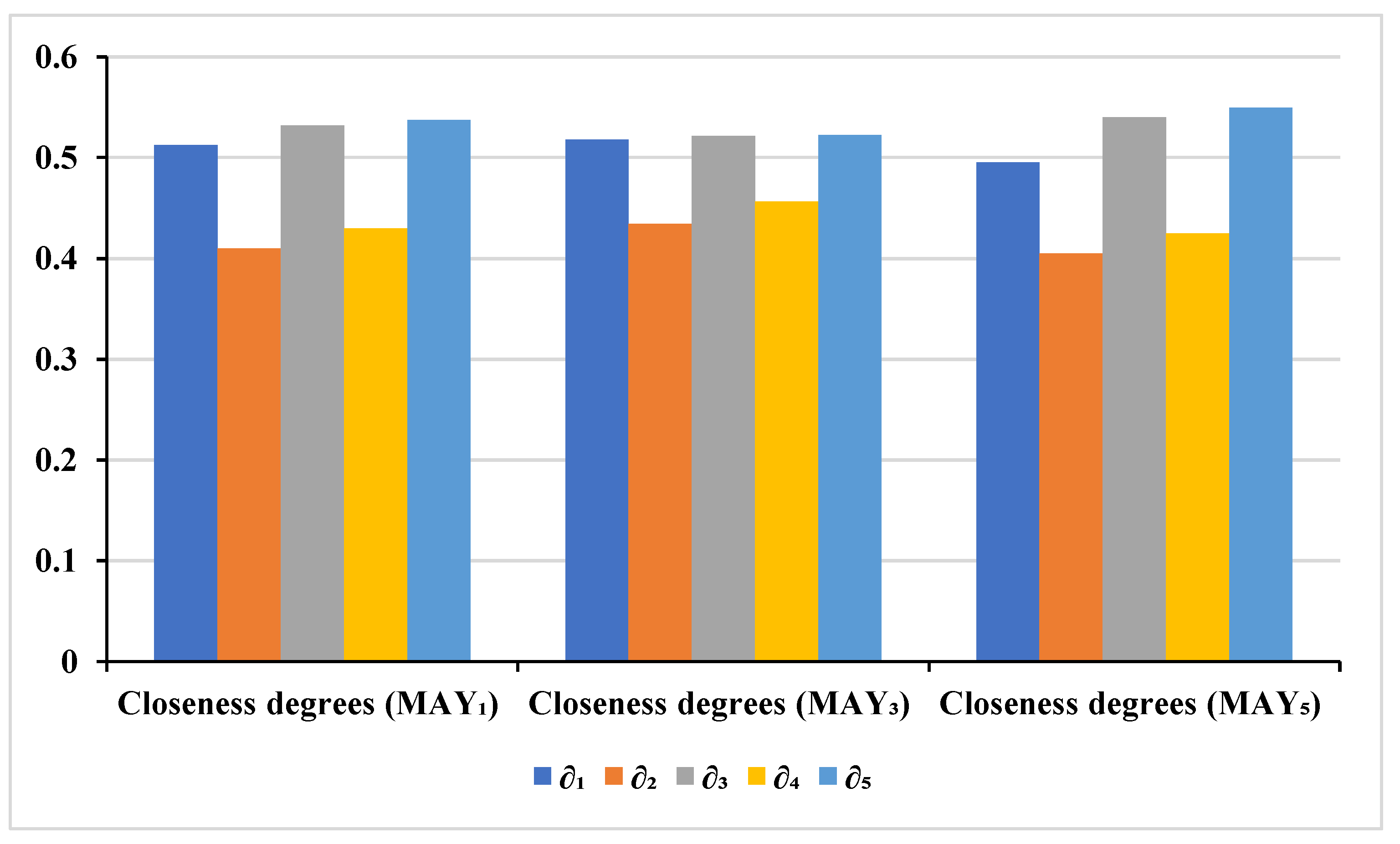
  $$\begin{gathered} {\partial }^{+}=\left(\langle 0.59,0.31,0.41;0.57\rangle ,\langle 0.56,0.32,0.41;0.50\rangle ,\langle 0.58,0.35,0.36;0.56\rangle ,\langle 0.57,0.28,0.37;0.63\rangle ,\langle 0.58,0.33,0.39;0.54\rangle \right), \\ {\partial }^{-}=\left(\langle 0.45,0.37,0.48;0.44\rangle ,\langle 0.49,0.44,0.45;0.45\rangle ,\langle 0.45,0.46,0.48;0.49\rangle ,\langle 0.48,0.42,0.51;0.48\rangle ,\langle 0.45,0.41,0.52;0.48\rangle \right). \end{gathered}$$
• Step 4. Computation of weighted Dis-Ms: Using Equations (47) and (48), we compute the weighted distances between the alternatives ${\partial }_i\left(i=1,2,\dots 5\right)$ and the G-TSF PIS ${\partial }^{+}$ as well as the G-TSF NIS ${\partial }^{-}$. The resultant distances are furnished in the following

  Table 9. Weighted distances from ${\partial }_i\left(i=1,2,\dots 5\right)$ to ${\partial }^{+}$ and ${\partial }^{-}$.

  Measures	Alternative
  	${\partial }_1$	${\partial }_2$	${\partial }_3$	${\partial }_4$	${\partial }_5$
  $Di{v}_{MA{Y}_1}^{\omega }\left({\partial }_i,{\partial }^{+}\right)$	0.002038	0.002973	0.002009	0.002711	0.001814
  $Di{v}_{MA{Y}_1}^{\omega }\left({\partial }_i,{\partial }^{-}\right)$	0.002246	0.001431	0.002595	0.001537	0.002446
  $G_{MA{Y}_1}^{\omega }\left({\partial }_i,{\partial }^{+}\right)$	0.04515	0.054522	0.044821	0.052068	0.042588
  $G_{MA{Y}_1}^{\omega }\left({\partial }_i,{\partial }^{-}\right)$	0.047397	0.037827	0.050944	0.039198	0.049458

  ,

  Table 10. Weighted distances from ${\partial }_i\left(i=1,2,\dots 5\right)$ to ${\partial }^{+}$ and ${\partial }^{-}$.

  Measures	Alternative
  	${\partial }_1$	${\partial }_2$	${\partial }_3$	${\partial }_4$	${\partial }_5$
  $Di{v}_{MA{Y}_3}^{\omega }\left({\partial }_i,{\partial }^{+}\right)$	0.024043	0.032561	0.023671	0.030376	0.023562
  $Di{v}_{MA{Y}_3}^{\omega }\left({\partial }_i,{\partial }^{-}\right)$	0.02771	0.019192	0.028078	0.021382	0.02814
  $G_{MA{Y}_3}^{\omega }\left({\partial }_i,{\partial }^{+}\right)$	0.155059	0.180447	0.153853	0.174286	0.1535
  $G_{MA{Y}_3}^{\omega }\left({\partial }_i,{\partial }^{-}\right)$	0.166463	0.138535	0.167566	0.146226	0.16775

  and

  Table 11. Weighted distances from ${\partial }_i\left(i=1,2,\dots 5\right)$ to ${\partial }^{+}$ and ${\partial }^{-}$.

  Measures	Alternative
  	${\partial }_1$	${\partial }_2$	${\partial }_3$	${\partial }_4$	${\partial }_5$
  $Di{v}_{MA{Y}_3}^{\omega }\left({\partial }_i,{\partial }^{+}\right)$	0.053204	0.073172	0.04757	0.067578	0.041995
  $Di{v}_{MA{Y}_3}^{\omega }\left({\partial }_i,{\partial }^{-}\right)$	0.051229	0.033811	0.065423	0.036844	0.062492
  $G_{MA{Y}_3}^{\omega }\left({\partial }_i,{\partial }^{+}\right)$	0.230661	0.270503	0.218107	0.259958	0.204926
  $G_{MA{Y}_3}^{\omega }\left({\partial }_i,{\partial }^{-}\right)$	0.226338	0.183878	0.255779	0.191948	0.249984

  , respectively.
• Step 5. Calculating RCDs ${\mathsf{\Theta }}_i$ and ranking of ${\partial }_i\left(i=1,2,\dots 5\right)$: We calculated the RCD ${\mathsf{\Theta }}_i$ of each alternative ${\partial }_i\left(i=1,2,\dots 5\right)$ to the G-TSF PIS ${\partial }^{+}$ using Equation (49). Finally, we rank the alternatives ${\partial }_i\left(i=1,2,\dots 5\right)$ in decreasing order of their RCD ${\mathsf{\Theta }}_i$ as shown in

  Table 12. RCD ${\mathsf{\Theta }}_i$ with a ranking of ${\partial }_i\left(i=1,2,\dots 5\right)$ for parameter $t=2$.

  Measures	Alternative
  	${\partial }_1$	${\partial }_2$	${\partial }_3$	${\partial }_4$	${\partial }_5$
  Closeness degrees ($MA{Y}_1$)	0.512141	0.409612	0.531965	0.429494	0.537314
  Ranking	${\partial }_5\succ {\partial }_3\succ {\partial }_1\succ {\partial }_4\succ {\partial }_2$
  Closeness degrees ($MA{Y}_3$)	0.517733	0.434305	0.521333	0.456226	0.522179
  Ranking	${\partial }_5\succ {\partial }_3\succ {\partial }_1\succ {\partial }_4\succ {\partial }_2$
  Closeness degrees ($MA{Y}_5$)	0.495271	0.404678	0.539749	0.424753	0.549525
  Ranking	${\partial }_5\succ {\partial }_3\succ {\partial }_1\succ {\partial }_4\succ {\partial }_2$

  , and select the alternative having the highest RCD ${\mathsf{\Theta }}_i$ as the most desirable alternative. Figure 5 below presents the order of ranking closeness degrees for $MA{Y}_1$, $MA{Y}_3$, and $MA{Y}_5$.

Thus, the step-by-step pseudocode summary is described in Algorithm 1.

Algorithm 1: Core 3-Step Div-M Computation

Input:  Fuzzy decision matrix from multiple experts.  Criteria weights.  Parameter t (sensitivity control). Step 1: Experts selection Experts are selected based on their professional credentials, field experience, and alignment with the project’s technical and environmental scope, including a Renewable Energy Specialist (Ph.D., 15+ years), an Electrical Engineer (M.Sc., 10 years), and an Environmental Scientist (M.Sc., 12 years). Step 2: Aggregate expert assessments  Aggregate expert assessments by using G-TSFs via:  $〈\overline{\stackrel{⌣}{\Im }},\overline{\stackrel{⌣}{\wp }},\overline{\stackrel{⌣}{\varphi }}〉=〈\sqrt[t]{{\displaystyle \frac{{\displaystyle \sum _{j=1}^n{\stackrel{⌣}{\Im }}_j^t}}{n}}},\sqrt[t]{{\displaystyle \frac{{\displaystyle \sum _{j=1}^n{\stackrel{⌣}{\wp }}_j^t}}{n}}},\sqrt[t]{{\displaystyle \frac{{\displaystyle \sum _{j=1}^n{\stackrel{⌣}{\varphi }}_j^t}}{n}}}〉$ and  $\stackrel{⌣}{r}=\min \left\{\underset{1\le j\le n}{\max }\sqrt{{({\overline{\stackrel{⌣}{\Im }}}^t-{\stackrel{⌣}{\Im }}_j^t)}^2+{({\overline{\stackrel{⌣}{\wp }}}^t-{\stackrel{⌣}{\wp }}_j^t)}^2+{({\overline{\stackrel{⌣}{\varphi }}}^t-{\stackrel{⌣}{\varphi }}_j^t)}^2},1\right\}$. Step 3: Compute distance measures and closeness indices For each alternative, calculate the distance to positive ideal and negative ideal solutions based on the proposed Div-Ms by using  $G_{MA{Y}_i}^{\omega }\left({\partial }_i,{\partial }^{+}\right)={\sqrt[t]{Di{v}_{MA{Y}_i}^{\omega }\left({\partial }_i,{\partial }^{+}\right)}}_{}$ and $G_{MA{Y}_i}^{\omega }\left({\partial }_i,{\partial }^{-}\right)=\sqrt[t]{Di{v}_{MA{Y}_i}^{\omega }\left({\partial }_i,{\partial }^{-}\right)}$  $\mathrm{where}, {\partial }^{+}=PIS=\left\{〈\stackrel{⌢}{e},\underset{1\le i\le n}{\max }{\stackrel{⌣}{\Im }}_{{\partial }_i}\left({\stackrel{⌢}{e}}_j\right),\underset{1\le i\le n}{\min }{\stackrel{⌣}{\wp }}_{{\partial }_i}\left({\stackrel{⌢}{e}}_j\right),\underset{1\le i\le n}{\min }{\stackrel{⌣}{\varphi }}_{{\partial }_i}\left({\stackrel{⌢}{e}}_j\right);\underset{1\le i\le n}{\max }{\stackrel{⌣}{r}}_{{\partial }_i}\left({\stackrel{⌢}{e}}_j\right)〉:\stackrel{⌢}{e}\in \stackrel{⌢}{E}\right\}$ and  ${\partial }^{-}=NIS=\left\{〈\stackrel{⌢}{e},\underset{1\le i\le n}{\min }{\stackrel{⌣}{\Im }}_{{\partial }_i}\left({\stackrel{⌢}{e}}_j\right),\underset{1\le i\le n}{\max }{\stackrel{⌣}{\wp }}_{{\partial }_i}\left({\stackrel{⌢}{e}}_j\right),\underset{1\le i\le n}{\max }{\stackrel{⌣}{\varphi }}_{{\partial }_i}\left({\stackrel{⌢}{e}}_j\right);\underset{1\le i\le n}{\min }{\stackrel{⌣}{r}}_{{\partial }_i}\left({\stackrel{⌢}{e}}_j\right)〉:\stackrel{⌢}{e}\in \stackrel{⌢}{E}\right\}$ are the positive ideal and negative ideal solutions, respectively. The closeness index is computed via  ${\mathsf{\Theta }}_i={\displaystyle \frac{G_{MA{Y}_i}^{\omega }\left({\partial }_i,{\partial }^{-}\right)}{G_{MA{Y}_i}^{\omega }\left({\partial }_i,{\partial }^{-}\right)+G_{MA{Y}_i}^{\omega }\left({\partial }_i,{\partial }^{+}\right)}}$. Step 4: Rank alternatives  Rank the alternatives in descending order of their closeness coefficients. Output: Final ranking of alternatives

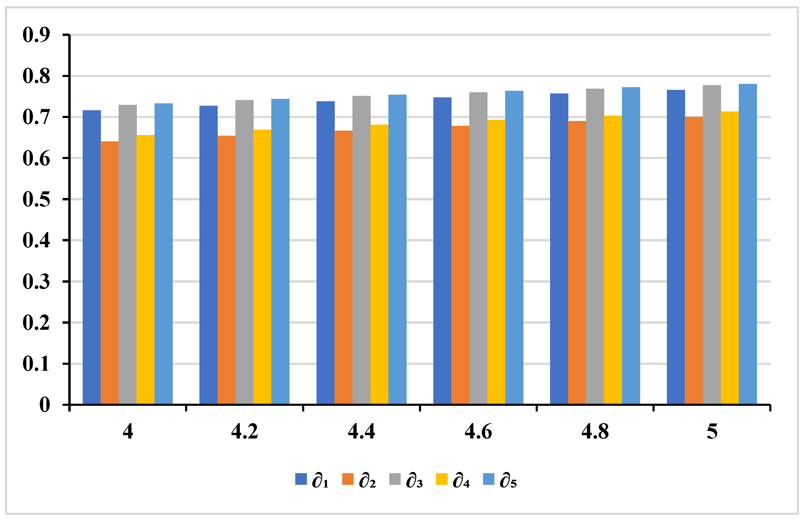
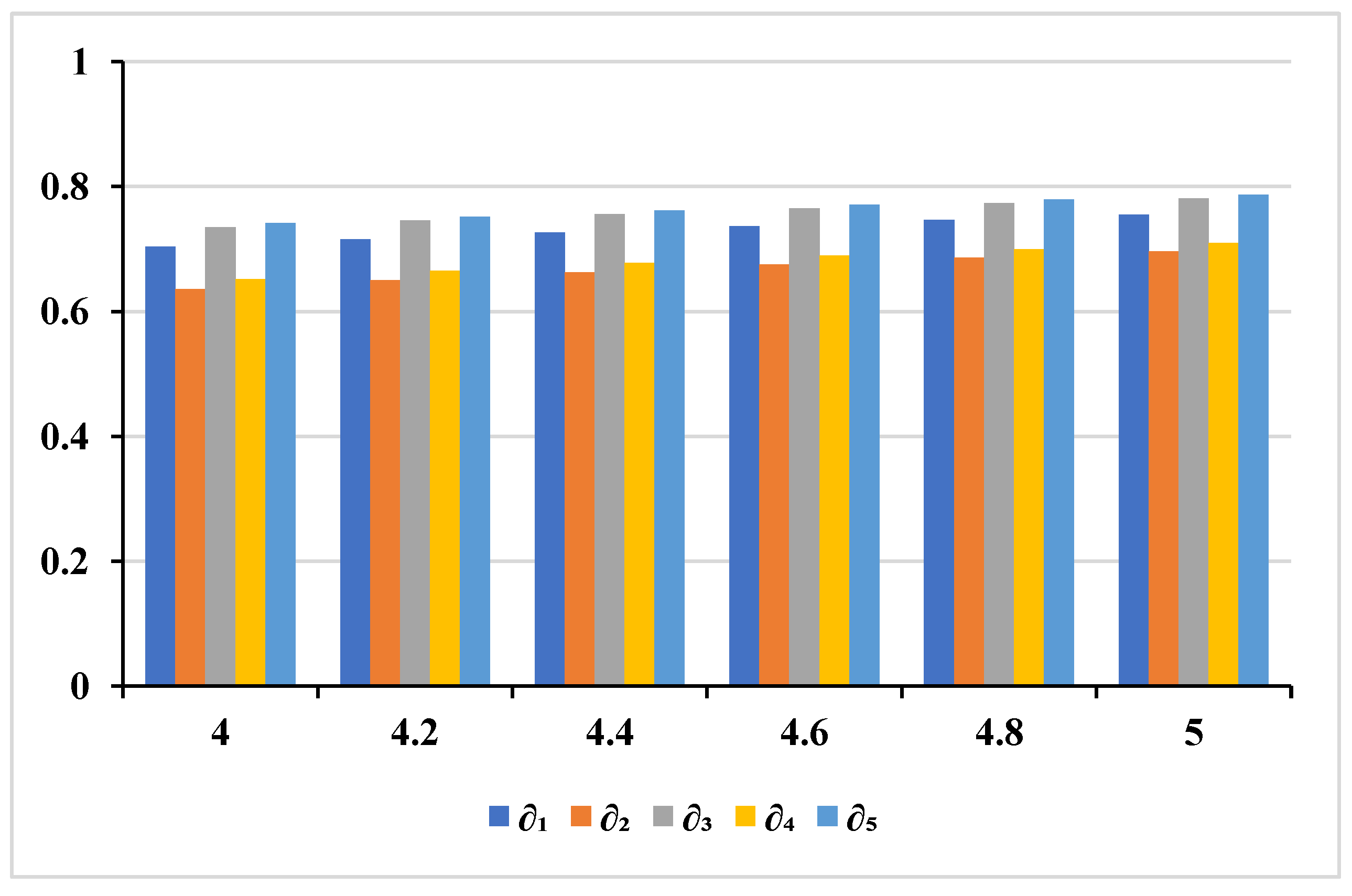
6. Sensitivity Analysis

To analyze the impact of the parameter $t$ on the D-M outcomes in Example 1, we utilize the proposed TOPSIS method, the RCD ${\mathsf{\Theta }}_i$ of each alternative ${\partial }_i$ for various values of the parameter $t$ ranging from 4.0 to 5.0, and the resultant values are presented in

Table 13. RCD ${\mathsf{\Theta }}_i$ for different values of $t$ using weighted $MA{Y}_1$.

$\mathit{t}$	Relative Closeness Degrees (RCD)					Ranking
	${\mathsf{\Theta }}_1$	${\mathsf{\Theta }}_2$	${\mathsf{\Theta }}_3$	${\mathsf{\Theta }}_4$	${\mathsf{\Theta }}_5$
4.0	0.71564	0.64001	0.72936	0.655358	0.733017	${\partial }_5\succ {\partial }_3\succ {\partial }_1\succ {\partial }_4\succ {\partial }_2$
4.2	0.727133	0.653756	0.740403	0.668679	0.743939	${\partial }_5\succ {\partial }_3\succ {\partial }_1\succ {\partial }_4\succ {\partial }_2$
4.4	0.737742	0.666509	0.750588	0.681024	0.754009	${\partial }_5\succ {\partial }_3\succ {\partial }_1\succ {\partial }_4\succ {\partial }_2$
4.6	0.747563	0.67837	0.760009	0.692494	0.763322	${\partial }_5\succ {\partial }_3\succ {\partial }_1\succ {\partial }_4\succ {\partial }_2$
4.8	0.75668	0.689428	0.768749	0.703179	0.771961	${\partial }_5\succ {\partial }_3\succ {\partial }_1\succ {\partial }_4\succ {\partial }_2$
5.0	0.765166	0.69976	0.776879	0.713153	0.779994	${\partial }_5\succ {\partial }_3\succ {\partial }_1\succ {\partial }_4\succ {\partial }_2$

,

Table 14. RCD ${\mathsf{\Theta }}_i$ for different values of $t$ using weighted $MA{Y}_3$.

$\mathit{t}$	RCD					Ranking
	${\mathsf{\Theta }}_1$	${\mathsf{\Theta }}_2$	${\mathsf{\Theta }}_3$	${\mathsf{\Theta }}_4$	${\mathsf{\Theta }}_5$
4.0	0.719537	0.659018	0.722034	0.675445	0.72262	${\partial }_5\succ {\partial }_3\succ {\partial }_1\succ {\partial }_4\succ {\partial }_2$
4.2	0.730904	0.672235	0.733319	0.688185	0.733885	${\partial }_5\succ {\partial }_3\succ {\partial }_1\succ {\partial }_4\succ {\partial }_2$
4.4	0.741393	0.684481	0.743731	0.699974	0.74428	${\partial }_5\succ {\partial }_3\succ {\partial }_1\succ {\partial }_4\succ {\partial }_2$
4.6	0.751101	0.695856	0.753367	0.710915	0.753898	${\partial }_5\succ {\partial }_3\succ {\partial }_1\succ {\partial }_4\succ {\partial }_2$
4.8	0.760112	0.706449	0.762309	0.721094	0.762825	${\partial }_5\succ {\partial }_3\succ {\partial }_1\succ {\partial }_4\succ {\partial }_2$
5.0	0.768498	0.716338	0.77063	0.730587	0.77113	${\partial }_5\succ {\partial }_3\succ {\partial }_1\succ {\partial }_4\succ {\partial }_2$

and

Table 15. RCD ${\mathsf{\Theta }}_i$ for different values of $t$ using weighted $MA{Y}_5$.

	RCD					Ranking
	${\mathsf{\Theta }}_1$	${\mathsf{\Theta }}_2$	${\mathsf{\Theta }}_3$	${\mathsf{\Theta }}_4$	${\mathsf{\Theta }}_5$
4.0	0.703755	0.636143	0.734676	0.65173	0.741299	${\partial }_5\succ {\partial }_3\succ {\partial }_1\succ {\partial }_4\succ {\partial }_2$
4.2	0.715628	0.649994	0.745542	0.665154	0.751942	${\partial }_5\succ {\partial }_3\succ {\partial }_1\succ {\partial }_4\succ {\partial }_2$
4.4	0.726595	0.662847	0.75556	0.677596	0.76175	${\partial }_5\succ {\partial }_3\succ {\partial }_1\succ {\partial }_4\succ {\partial }_2$
4.6	0.736755	0.674805	0.764824	0.68916	0.770817	${\partial }_5\succ {\partial }_3\succ {\partial }_1\succ {\partial }_4\succ {\partial }_2$
4.8	0.746193	0.685955	0.773416	0.699933	0.779222	${\partial }_5\succ {\partial }_3\succ {\partial }_1\succ {\partial }_4\succ {\partial }_2$
5.0	0.754983	0.696376	0.781406	0.709994	0.787037	${\partial }_5\succ {\partial }_3\succ {\partial }_1\succ {\partial }_4\succ {\partial }_2$

. As evident from these tables, the ranking orders of the alternatives remain consistent when the parameter $t$ varies from 4.0 to 5.0. This observation allows us to confidently assert that SES-5 (${\partial }_5$) is the optimal SES, as its ranking remains unaffected by the changes in the value of parameter $t$. Figure 6, Figure 7 and Figure 8 illustrate the weighted ranking order of the alternative based on closeness degrees for $MA{Y}_1$, $MA{Y}_3$, and $MA{Y}_5$ under different values of the parameter $t$.

7. Conclusions

Divergence measures are essential in distinguishing between complex data structures, especially in fuzzy decision-making environments where uncertainty and granularity are significant. Despite considerable progress in the field, the formulation of divergence measures for Globular T-Spherical Fuzzy Sets (G-TSFSs), particularly within the context of multi-criteria group decision-making (MCGDM), has remained underdeveloped. This study addresses that gap by introducing a novel suite of divergence measures (Div-Ms) specifically designed for G-TSFSs, supported by rigorous theoretical analysis. These Div-Ms form the basis for new distance and similarity measures, providing a cohesive mathematical foundation for advanced decision-making models. We have operationalized these constructs into a robust G-TSF-TOPSIS framework, which is applied to the practical task of selecting optimal solar energy systems (SESs) for a university context. The model, incorporating equally weighted expert evaluations, demonstrates resilience through sensitivity analysis over the tunable parameter “$t$“ (4.0–5.0 with an increment of 0.2), showing stable decision outcomes. Comparative results with existing methods affirm the superiority, stability, and practical utility of the proposed approach in handling complex, uncertain decision environments. This work contributes both theoretically and practically to fuzzy set theory and decision science, offering a valuable foundation for future research. Nonetheless, the study is limited by the assumption of equal expert weights and a single application domain. Future work may explore dynamic expert weighting strategies and apply the model to broader, cross-sectoral decision-making scenarios to enhance generalizability and impact. Additionally, hybridizing the framework with optimization algorithms or machine learning techniques could support adaptive and automated decision systems in smart grid environments. Exploring interdependent criteria using advanced fuzzy aggregation operators, and applying the model to diverse case studies such as renewable energy project selection, energy policy planning, and sustainable resource allocation, will further validate and expand its practical utility.

References

1. Zadeh, L.A. Fuzzy Sets. Inf. Control 1965, 8, 338–356. [Google Scholar] [CrossRef]
2. Pozna, C.; Precup, R.E.; Horvath, E. Hybrid particle filter–particle swarm optimization algorithm and application to fuzzy controlled servo systems. IEEE Trans. Fuzzy Syst. 2022, 30, 4286–4297. [Google Scholar] [CrossRef]
3. Azeem, M.; Anwar, S.; Jamil, M.K.; Saeed, M.; Deveci, M. Topological numbers of fuzzy soft graphs and their application. Inf. Sci. 2024, 667, 120468. [Google Scholar] [CrossRef]
4. Chen, H.; Gao, X.; Wu, Q. An enhanced fuzzy time series forecasting model integrating fuzzy c-means clustering, the principle of justifiable granularity, and particle swarm optimization. Symmetry 2025, 17, 753. [Google Scholar] [CrossRef]
5. Atanassov, K.T. Intuitionistic fuzzy sets. Fuzzy Sets Syst. 1986, 20, 87–96. [Google Scholar] [CrossRef]
6. Hwang, C.M.; Yang, M.S. New construction for similarity measures between intuitionistic fuzzy sets based on lower, upper and middle fuzzy sets. Int. J. Fuzzy Syst. 2013, 15, 359–366. [Google Scholar]
7. Garg, H.; Kumar, K. Linguistic interval-valued Atanassov intuitionistic fuzzy sets and their applications to group decision making problems. IEEE Trans. Fuzzy Syst. 2019, 27, 2302–2311. [Google Scholar] [CrossRef]
8. Joshi, R.; Kumar, S. An intuitionistic fuzzy (δ, γ)-norm entropy with its application in supplier selection problem. Comput. Appl. Math. 2018, 37, 5624–5649. [Google Scholar] [CrossRef]
9. Cuong, B.C. Picture fuzzy sets. J. Comput. Sci. Cybern. 2014, 30, 409–420. [Google Scholar]
10. Wei, G. Picture fuzzy cross-entropy for multiple attribute decision making problems. J. Bus. Econ. Manag. 2016, 17, 491–502. [Google Scholar] [CrossRef]
11. Wang, L.; Zhang, H.Y.; Wang, J.Q.; Li, L. Picture fuzzy normalized projection-based VIKOR method for the risk evaluation of construction project. Appl. Soft Comput. 2018, 64, 216–226. [Google Scholar] [CrossRef]
12. Maji, P.K.; Roy, A.R.; Biswas, R. Soft set theory. Comput. Math. Appl. 2003, 45, 555–562. [Google Scholar] [CrossRef]
13. Smarandache, F. Extension of soft set to hypersoft set, and then to plithogenic hypersoft set. Neutrosophic Sets Syst. 2018, 22, 168–170. [Google Scholar]
14. Saqlain, M.; Riaz, M.; Saleem, M.A.; Yang, M.S. Distance and similarity measures for neutrosophic hypersoft set (NHSS) with construction of NHSS-TOPSIS and applications. IEEE Access 2021, 9, 30803–30816. [Google Scholar] [CrossRef]
15. Jafar, M.N.; Saeed, M.; Saqlain, M.; Yang, M.S. Trigonometric similarity measures for neutrosophic hypersoft sets with application to renewable energy source selection. IEEE Access 2021, 9, 129178–129187. [Google Scholar] [CrossRef]
16. Mahmood, T.; Ullah, K.; Khan, Q.; Jan, N. An approach toward decision-making and medical diagnosis problems using the concept of spherical fuzzy sets. Neural Comput. Appl. 2019, 31, 7041–7053. [Google Scholar] [CrossRef]
17. Ullah, K.; Mahmood, T.; Jan, N. Similarity measures for T-spherical fuzzy sets with applications in pattern recognition. Symmetry 2018, 10, 193. [Google Scholar] [CrossRef]
18. Abid, M.N.; Yang, M.S.; Karamti, H.; Ullah, K.; Pamucar, D. Similarity measures based on T-spherical fuzzy information with applications to pattern recognition and decision making. Symmetry 2022, 14, 410. [Google Scholar] [CrossRef]
19. Tran, T.H.; Nguyen, P.H.; Nguyen, L.A.T.; Nguyen, T.H.T. Understanding the complexities: Interrelationships of critical barriers to university technology transfer in Vietnam using T-spherical fuzzy MCDM Approach. IEEE Access 2024, 12, 169683–169719. [Google Scholar] [CrossRef]
20. Rani, P.; Mishra, A.R.; Mardani, A.; Cavallaro, F.; Štreimikienė, D.; Khan, S.A.R. Pythagorean fuzzy SWARA–VIKOR framework for performance evaluation of solar panel selection. Sustainability 2020, 12, 4278. [Google Scholar] [CrossRef]
21. Kumar, N.; Mahanta, J. A matrix norm-based Pythagorean fuzzy metric and its application in MEREC-SWARA-VIKOR framework for solar panel selection. Appl. Soft Comput. 2024, 158, 111592. [Google Scholar] [CrossRef]
22. Hamdy, M.; Ibrahim, A.; Abozalam, B.; Helmy, S. Design and implementation of Type-3 intuitionistic fuzzy logic MPPT controller for PV solar system: Comparative study. ISA Trans. 2024, 154, 488–511. [Google Scholar] [CrossRef] [PubMed]
23. Ashraf, S.; Jana, C.; Sohail, M.; Choudhary, R.; Ahmad, S.; Deveci, M. Multi-criteria decision-making model based on picture hesitant fuzzy soft set approach: An application of sustainable solar energy management. Inf. Sci. 2025, 686, 121334. [Google Scholar] [CrossRef]
24. Atanassov, K.T. Circular intuitionistic fuzzy sets. J. Intell. Fuzzy Syst. 2020, 39, 5981–5986. [Google Scholar] [CrossRef]
25. Atanassov, K.; Marinov, E. Four distances for circular intuitionistic fuzzy sets. Mathematics 2021, 9, 1121. [Google Scholar] [CrossRef]
26. Garg, H.; Ünver, M.; Olgun, M.; Türkarslan, E. An extended EDAS method with circular intuitionistic fuzzy value features and its application to multi-criteria decision-making process. Artif. Intell. Rev. 2023, 56 (Suppl. S3), 3173–3204. [Google Scholar] [CrossRef]
27. Alreshidi, N.A.; Shah, Z.; Khan, M.J. Similarity and entropy measures for circular intuitionistic fuzzy sets. Eng. Appl. Artif. Intell. 2024, 131, 107786. [Google Scholar] [CrossRef]
28. Bozyiğit, M.C.; Olgun, M.; Ünver, M. Circular Pythagorean fuzzy sets and applications to multi-criteria decision making. Informatica 2023, 34, 713–742. [Google Scholar] [CrossRef]
29. Yusoff, B.; Kilicman, A.; Pratama, D.; Hasni, R. Circular q-rung orthopair fuzzy set and its algebraic properties. Malays. J. Math. Sci. 2023, 17, 363–378. [Google Scholar] [CrossRef]
30. Ying, G. Mental health assessment model for college students using circular q-rung orthopair fuzzy Muirhead means and MULTIMOORA method. IEEE Access 2025, 13, 35433–35451. [Google Scholar] [CrossRef]
31. Ashraf, S.; Iqbal, W.; Ahmad, S.; Khan, F. Circular spherical fuzzy Sugeno Weber aggregation operators: A novel uncertain approach for adaption a programming language for social media platform. IEEE Access 2023, 11, 124920–124941. [Google Scholar] [CrossRef]
32. Ashraf, S.; Jana, C.; Iqbal, W.; Deveci, M. Regret-based domination three-way decision-making model with circular spherical fuzzy Mahalanobis distance. Inf. Sci. 2025, 691, 121616. [Google Scholar] [CrossRef]
33. Ashraf, S.; Chohan, M.S. Circular spherical fuzzy aggregation operators: A case study of risk assessments on industry expansion. Eng. Appl. Artif. Intell. 2025, 145, 110202. [Google Scholar] [CrossRef]
34. Yang, M.S.; Akhtar, Y.; Ali, M. On globular T-spherical fuzzy (G-TSF) sets with application to G-TSF multi-criteria group decision-making. arXiv 2024, arXiv:2403.07010. [Google Scholar]
35. Bhandari, D.; Pal, N.R.; Majumder, D.D. Fuzzy divergence, probability measure of fuzzy events and image thresholding. Pattern Recognit. Lett. 1992, 13, 857–867. [Google Scholar] [CrossRef]
36. Chaira, T.; Ray, A.K. Segmentation using fuzzy divergence. Pattern Recognit. Lett. 2003, 24, 1837–1844. [Google Scholar] [CrossRef]
37. Wu, M.Q.; Chen, T.Y.; Fan, J.P. Divergence measure of T-spherical fuzzy sets and its applications in pattern recognition. IEEE Access 2019, 8, 10208–10221. [Google Scholar] [CrossRef]
38. Khan, M.J.; Kumam, W.; Alreshidi, N.A. Divergence measures for circular intuitionistic fuzzy sets and their applications. Eng. Appl. Artif. Intell. 2022, 116, 105455. [Google Scholar] [CrossRef]
39. Zhu, S.; Liu, Z.; Ulutagay, G.; Deveci, M.; Pamucar, D. Novel α-divergence measures on picture fuzzy sets and interval-valued picture fuzzy sets with diverse applications. Eng. Appl. Artif. Intell. 2024, 136, 109041. [Google Scholar] [CrossRef]
40. Khan, F.M.; Munir, A.; Albaity, M.; Nadeem, M.; Mahmood, T. Software reliability growth model selection by using VIKOR method based on q-rung orthopair fuzzy entropy and divergence measures. IEEE Access 2024, 12, 86572–86582. [Google Scholar] [CrossRef]
41. Riaz, M.; Habib, A.; Saqlain, M.; Yang, M.S. Cubic bipolar fuzzy VIKOR method using new distance and entropy measures and Einstein averaging aggregation operators with application to renewable energy. Int. J. Fuzzy Syst. 2023, 25, 510–543. [Google Scholar] [CrossRef]
Figure 1. Layout of the paper.
Symmetry 17 00872 g001
Figure 2. The proposed G-TSF TOPSIS model.
Symmetry 17 00872 g002
Figure 3. Workflow of the proposed methodology.
Symmetry 17 00872 g003
Figure 4. G-TSFDM process.
Symmetry 17 00872 g004
Figure 5. Ranking of closeness degrees.
Symmetry 17 00872 g005
Figure 6. Ranking of alternatives based on RCD using weighted M A Y 1 for different values of the parameter t .
Symmetry 17 00872 g006
Figure 7. Ranking of alternatives based on RCD using weighted M A Y 3 for different values of the parameter t .
Symmetry 17 00872 g007
Figure 8. Ranking of alternatives based on RCD using weighted M A Y 5 for different values of the parameter t .
Symmetry 17 00872 g008