1. Introduction
Real-world decision making often involves uncertainty due to imprecise or incomplete information. Fuzzy sets, introduced by Zadeh in 1965 [
1], were developed to tackle these challenges. They represent the degree of certainty for an element’s inclusion in a decision using membership functions or degree (MD). However, assigning precise degrees can be difficult in many situations due to various factors such as limited information [
2,
3], conflicting evidence [
4,
5,
6], or time constraints [
7,
8]. Classical sets A are extended by intuitionistic fuzzy sets (IFSs), which introduce the notions of membership degree (MD) and non-membership degree (NMD). Atanassov introduced them in 1986 [
9,
10]. Compared to conventional crisp sets, IFS provides a more potent way to convey ambiguity and uncertainty. Scientists have made significant advancements in applying IFSs to problems characterized by ambiguity [
11]. These techniques provide robust frameworks for consolidating information, assessing correlation, and facilitating decision making in domains where exact information may be inaccessible or ambiguous [
12]. Furthermore, the basic IFS theory is still being developed and applied in real-world situations thanks to the continued exploration of extensions and changes [
13]. IFSs have been used in many real-world applications, from finance and technology to medical and managing the environment, due to their adaptability and efficacy [
14]. By adding the idea of uncertainty through the usage of MDs and NMDs, Yager [
15] established a Pythagorean fuzzy set (PFSs), which is a form of FS that extends classical sets A and incorporates an extra level of doubt indicated by the degree of hesitation. Yager’s contributions [
16] represent important developments in the use of PF sets in aggregation operations, especially the invention of the PF Weighted Averaging (PFWA) operator and the PF Ordered Weighted Averaging (PFOWA) operator. Yager extended the capabilities of aggregation techniques to handle uncertain and vague information more effectively. Building on this work, Peng and Yang [
17] extended the use of PF sets to information aggregation by incorporating the Choquet integral. Zhang and Xu [
18] proposed that the application involves utilizing the TOPSIS method with PFNs. The q-rung orthopair fuzzy set (q-ROFS) was first introduced by Yagar [
19], and their concept is used in MCDM and other fields requiring uncertainty modeling and information processing. This concept extends intuitionistic fuzzy sets (IFSs) and Pythagorean fuzzy sets (PFSs) by allowing a higher degree of freedom in representing uncertainty. The q-ROFS can be applied to various fields such as decision making [
20], medical diagnosis [
21], risk assessment [
22], and more.
Recent advancements in fuzzy set theory have significantly enhanced our ability to model complex uncertainty and ambiguity. Remote et al. [
23] introduced the concept of complex fuzzy sets (CFSs), which extend traditional fuzzy sets (FSs) by incorporating complex numbers for membership degrees (MDs). This innovation allows for a more nuanced representation of uncertainty, particularly in dynamic and oscillatory systems where phase information is crucial. Building on this foundation, Parvathi et al. [
24] proposed Complex Intuitionistic Fuzzy Sets (CIFSs), which further expand intuitionistic fuzzy sets by using complex numbers for both MDs and non-membership degrees (NMDs). This extension provides greater flexibility in modeling situations where hesitation and partial truth coexist [
25,
26]. To address even more intricate scenarios, Peng et al. [
27,
28] developed complex Pythagorean fuzzy sets (CPFSs), which generalize Pythagorean fuzzy sets by allowing MDs and NMDs to be complex numbers. More recently, Liao et al. [
29] introduced complex q-rung orthopair fuzzy sets (Cq-ROFSs), which enhance the modeling of uncertainty and imprecision in data. Cq-ROFSs are particularly valuable in applications requiring high levels of detail and precision, as they represent MDs and NMDs as complex numbers [
30,
31]. These developments collectively provide a robust framework for handling uncertainty in multi-criteria decision-making (MCDM) scenarios.
The Choquet integral operator, first introduced in [
32] and further explored in [
33] in the context of fuzzy measures, serves as a powerful tool for evaluating interactions between decision alternatives. It enables the calculation of expected utility in uncertain scenarios. Building on this foundation, Tan and Chen introduced the intuitionistic fuzzy Choquet integral (IFCI) operator [
34], enhancing the modeling of uncertain information. Wei later expanded this work by proposing the interval-valued intuitionistic fuzzy Choquet integral (IVIFCI) operator [
35], incorporating interval-valued membership and non-membership degrees for greater flexibility. Meng and Tan further advanced the field by developing methods for extended interval-valued intuitionistic fuzzy sets with generalized association variables [
36]. The Shapley function, first presented in [
37], offers a structured method to account for the importance of ordered elements in decision making through the Choquet integral. For a deeper understanding of the Shapley function and its applications, refer to [
38,
39,
40,
41], which explore aggregation operators based on this function, particularly in interdependent decision-making contexts. Qin et al. [
42] also contributed by proposing interval-valued intuitionistic fuzzy measures that integrate fuzzy entropy and Shapley values. Triangular norms (t-NMs) and triangular conorms (t-CNMs), introduced by Menger [
43], are fundamental to the functioning of intuitionistic fuzzy sets (IFSs). Various types of these norms, such as Einstein [
44], Archimedean [
45], Lukasiewicz [
46], and Hamacher [
47], have been developed to enhance fuzzy systems. Klement and Mesiar [
48] provided a thorough analysis of these norms in 2000. Additionally, Aczel and Alsina [
49] introduced the Aczel–Alsina t-NM and t-CNM, which offer increased flexibility in fuzzy systems through their parameterized operations.
Recent studies have explored various aggregation operators in fuzzy environments. For instance, a fuzzy-based evaluation method was employed in [
50] to assess the impact of e-learning on ICT students during the COVID-19 lockdown in Greece. The study analyzed four criteria—acceptance, learning effectiveness, engagement, and socializing—using fuzzy logic to interpret Likert-scale responses from 92 students and 10 instructors. The fuzzy rule-based system (209 rules) mimicked human reasoning, enhancing interpretability. Addressing the need for personalized e-learning, the author of [
51] proposed a fuzzy-based adaptive system for programming language education. Their framework employs fuzzy cognitive maps (FCMs) to model concept dependencies and fuzzy rules to dynamically recommend content based on learners’ knowledge levels. The authors of [
52] proposed a confidence-based e-learning system, and this system uses an artificial neural network to find the cognitive state of the e-learner based on the performance in the test.
1.1. Motivation
The motivation behind using CIFSs in MCDM lies in their unique ability to handle uncertainty and periodicity in data. CIFSs extend traditional fuzzy sets by incorporating complex numbers for membership and non-membership degrees, allowing for a more nuanced representation of information. This is particularly valuable in real-world applications such as engineering design, where symmetry considerations impact stability, aesthetics, and environmental integration. The proposed model’s complexity is justified by its capacity to capture intricate interactions and uncertainties that simpler models might overlook.
Novelty of Aczel–Alsina Operators: While aggregation operators like Dombi, Frank, and Archimedean have been extensively studied and applied in various fuzzy environments, the Aczel–Alsina operators offer distinct advantages that make them particularly suitable for certain complex decision-making scenarios. Unlike Dombi operators, which are based on a specific family of functions that can be sensitive to parameter selection, Aczel–Alsina operators provide a more flexible framework for modeling the interaction between criteria through their unique parameterization. Frank operators, known for their ability to generalize probabilistic sums and products, are limited in capturing the full spectrum of interactions that can occur in multi-criteria settings. Archimedean operators, though widely used for their smooth transition properties, may not adequately represent the non-linear interactions and the dynamic range of uncertainties present in real-world data. Recent advancements in fuzzy aggregation operators, such as the intuitionistic Dombi aggregation operator, picture fuzzy Frank aggregation operators, and q-rung orthopair Archimedean aggregation operators, have significantly contributed to the field by enhancing the modeling of hesitation and partial truths in decision-making processes. However, these operators often focus on specific aspects of uncertainty and may not fully address the complex interdependencies and periodic uncertainties that are characteristic of certain applications, such as those involving oscillatory or phase-dependent data. The Aczel–Alsina operators, with their inherent flexibility and ability to model a wide range of interactions, fill this gap by providing a more comprehensive and adaptable tool for aggregating information in environments where both the nature of uncertainty and the relationships between criteria are intricate and multifaceted. This makes them an ideal choice for developing robust decision-making frameworks in fields such as engineering, finance, and healthcare, where the ability to accurately model and integrate diverse and complex information sources is crucial for effective decision support.
1.2. Objectives
The objectives of this essay are as follows:
To investigate the fundamental procedures of AAGSCI aggregation formulas using CIF data.
To provide the framework of the AAGSCI while taking IF data into account along with a few suitable features.
To devise several novel methodologies, including CIFAAWAGSCI, GCIFAAWGGSCI , GCIFAAWAGSCI, GCIFAAOWAGSCI, CIFAAOWAGSCI, GCIFAAOWGGSCI, CIFAAWGGSCI, and CIFAAOWGGSCI operators, which possess certain features.
To assess the versatility and efficiency of AOs by providing a case study using numerical examples from the building and engineering administration sectors.
To conduct a thorough comparative analysis, evaluating current AOs with old AOs and drawing a conclusion.
1.3. Structure of the Paper
The remainder of this paper is structured as follows:
Section 2 introduces fundamental concepts in fuzzy set theory, Aczel–Alsina operations, and the Choquet integral, establishing the groundwork for the proposed operators.
Section 3 presents the novel CIFAAWAGSCI and CIFAAWGGSCI operators and their generalized forms (GCIFAAWAGSCI, etc.), including an analysis of their key mathematical properties.
Section 4 explores the computational characteristics and interpretability of the proposed operators.
Section 5 applies the developed approach to numerical examples and an industrial case study.
Section 6 compares the GCIFAAGSCI and CIFAAGSCI models, providing a complete MCDM procedure.
Section 7 includes a sensitivity analysis, and
Section 8 concludes the paper with findings, practical implications, and future research directions.
2. Preliminaries
To prepare for their practical application in later sections, this section provides a review of key definitions and operations related to IFSs, CIFSs, fuzzy measures, the Choquet integral, the Shapley Choquet integral, and the Aczel–Alsina operator, laying the groundwork for their application in the subsequent sections.
Definition 1. An intuitionistic fuzzy set (IFS) [9] called A on a finite set consists of elements x from and their corresponding membership degrees () and non-membership degrees (). This is represented mathematically aswhere both MD and NMD are numerical values between 0 and 1, representing their strength. They satisfy a specific constraint: for all elements in X. This ensures that the sum of these degrees never exceeds 1, representing their complementary nature. Definition 2. An CIFS [27] called A on a finite set consists of element x from and their corresponding MD () and NMD (). This is represented mathematically aswhere both MD and NMD are numerical values between 0 and 1, representing their strength. , . They satisfy a specific constraint: for all elements in X. and . Definition 3 ([
33]).
Assume a fuzzy measure denoted by ¥ on a finite set called . FMs ¥ are mathematical tools used to represent the importance or value of subsets within a set with values between 0 (no importance) and 1 (full importance) and a mapping , satisfying the following:;
if , then .
In multi-criteria decision making with
n criteria, defining a general fuzzy measure requires
coefficients, making the model complex and computationally expensive. Sugeno [
34] introduced the
-fuzzy measure as a special type of fuzzy measure that reduces this complexity. The
-fuzzy measure requires only one parameter,
, to define the importance of each set of criteria. This reduces the number of coefficients needed from
to just 1, significantly simplifying the model. Despite its simplicity, the
-fuzzy measure can still capture various interaction effects between criteria, depending on the value of
.
Definition 4 ([
33]).
Assume that is a finite set with fuzzy measure σ then a mapping , satisfying the following:;
if , then ;
, ; and .
More specifically, the condition (iii) simplifies to the additive measure axiom if
:
When every element in
is independent as it is in this instance, we have
Definition 5. Assume that is a non-empty set; then, the Sugeno FMs [33] for any subset as defined arewhen , then it becomes Definition 6. Assume that is a non-empty set and ; then, the GSI [37] is defined as shown below: ¥: fuzzy measure on set N.
: cardinality of set N.
: cardinality of subset Q.
: cardinality of subset T.
: value assigned to the union of subsets Q and T under the fuzzy measure.
: value assigned to subset T under the fuzzy measure.
Furthermore, when , then , and the GSI reduces to the SF [37] as shown below: Equation (
5) yields
if for each coalition
because of  having no connection among the combination of
Q and any permutation of coalition
. Furthermore, if
for all
, it is evident that according to the fuzzy measure Definition 4,
and
with
. The weight vector linked to component
is thus represented by
.
The GSI considers both the individual contribution of an element and its interaction with other elements in different subsets. If there is no interaction between elements and subsets, the GSI reduces to the value of the individual element or subset under the fuzzy measure. The GSI weights assigned to all elements always sum to 1, representing a weight vector for the set. The GSI ensures that the sum of all element weights equals 1, representing the total value within the set. If we have two disjoint sets, the GSI of their union is equal to the sum of individual GSIs for each set. If an element has no interaction with any other element or subset, its GSI equals 0.
Definition 7. Assume that is a non-empty set, , a set of n elements , and f is a function assigned to each element of that set. Additionally, an ¥ is defined on , where ¥ . The discrete Choquet integral (denoted by ) is defined as Aczel–Alsina Operations for CIFEs
In this section, we define the AA operational laws for the CIFVs [
25]. These operations are specifically designed to work with CIFNs, which are a type of fuzzy set used to represent imprecise or uncertain information.
Definition 8. Assume that and are three CIFEs, as well as . Then, the AA operational laws on CIFEs are shown below:
3. The Generalized CIF-AA Average Generalized SCI Operator and Their Special Case
In this section, we discuss the GCIFAASCI operators and their special casses. These include the GCIFAA Weighted Average GSCI (GCIFWAGSCI) operator, GCIFAA Ordered Weighted Average GSCI (GCIFAAOWAGSCI) operator, GCIFAA Weighted Geometric GSCI (GIFWGGSCI) operator, and GIFAA Ordered Weighted Geometric GSCI (GCIFAAOWGGSCI) operator.
3.1. The Generalized CIF-AA Average Generalized SCI (GIFAAAGSCI) Operators
In this section, we discuss the GCIFAA Weighted Average GSCI operator (GCIFWAGSCI) and GCIFAA Ordered Weighted Average GSCI (GCIFAAOWAGSCI) operator.
Definition 9. Assume are on ¥ and is an FM; then, the iswhere and denote the AA sum. Theorem 1. Suppose are . Then, GCIFAAAGSCI is shown below:
Proof. By the induction method, for
, then
and
Based on the above definition, we obtain
So, the equation is true for
Now, let Equation (1) be true for
, such that
Now, for , we have
So, Equation (
1) is also true for
So, from all of the above calculations, we conclude that it also proves for
. □
Theorem 2 (Idempotency property).
Assume are . Then, Proof. As
are
. Then,
Thus, . □
Theorem 3 (Boundedness property).
Assume are , and let as well as . Then, GCIFAAAGSCI is defined as Proof. Let
be
, and also let
and
with
and
. Then,
is shown below:
and
we obtain
□
Theorem 4 (Monotonicity property).
Let and ∀ ) be , and if ), then Proof. This is similar to Theorem 2. □
3.2. CIF-AA Ordered Average Generalized SCI (IFAAOAGSCI) Operators
In this section, we discuss the GCIFAA Ordered Weighted Average GSCI (GCIFAAOWAGSCI) operators.
Definition 10. Suppose are with mapping : Then, the operator is shown below:where denote the permutation. Theorem 5. Suppose are . Then, the operator iswhere denotes the permutation. Proof. This is similar to Theorem 2. □
Theorem 6 (Idempotency property).
Suppose are . Then, Proof. This is similar to Theorem 3. □
Theorem 7 (Boundedness property).
Assume that are , and
and . Then, GCIFAAOAG SCI is shown below: Proof. This is similar to Theorem 4. □
Theorem 8 (Monotonicity property).
Suppose and are . Then, Proof. This is similar to Theorem 5. □
Theorem 9 (Commutativity property).
Let and be . Then,where represents the permutation. Definition 11. Let be and mapping : Then, a operator is shown below:where denotes permutation. Theorem 10. Assume that are . Then, the operator has the following form:
where denotes the permutation. 4. The Generalized CIF-AA Geometric Generalized SCI Operator and Their Special Case
In this section, we discuss the GCIFAASCI operators and their special casses. These include the GCIFAA Weighted Average GSCI operator (GCIFWAGSCI), GCIFAA Ordered Weighted Average GSCI (GCIFAAOWAGSCI) operator, GCIFAA Weighted Geometric GSCI operator (GCIFWGGSCI), and GIFAA Ordered Weighted Geometric GSCI (GCIFAAOWGGSCI) operator.
4.1. The Generalized CIF-AA Geometric Generalized SCl GIFAAGGSCI Operators
In this section, we discuss the GCIFAA weighted geometric GSCI operator (GCIFWGGSCI) and GCIFAA ordered weighted geometric GSCI (GCIFAAOWGGSCI) operator.
Definition 12. Assume Γ is a finite set and ¥
is an FM on Γ. Assume are ; then, the operator iswhere . Theorem 11. Let be . Then, the operator is shown below: Theorem 12 (Idempotency property).
Suppose are , ∀ .
Then, Γ.
Theorem 13 (Boundedness property).
Assume that are , and let and . Then, is defined as Theorem 14 (Monotonicity property).
Consider , and , ) as , and if ), then Proof. This is similar to Theorem 2. □
4.2. The Generalized CIF-AA Ordered Geometric Generalized SCl GIFAAGGSCI Operators
In this section, we discuss the GCIFAA Ordered Weighted Geometric GSCI (GCIFAAOWGGSCI) operator.
Definition 13. Assume that are and mappng : The is defined as shown below: Theorem 15. Assume that are C. Then, the operator is shown below: Proof. This is similar to Theorem 2. □
Theorem 16 (Idempotency property).
Assume that are . Then, Proof. This is similar to Theorem 3. □
Theorem 17 (Boundedness property).
Assume that are , and also Then, Proof. This is similar to Theorem 4. □
Theorem 18 (Monotonicity property).
Assume that as well as , ) are two . Then, Proof. This is similar to Theorem 5. □
Theorem 19 (Commutativity property).
Assume that as well as , as the two . Then, Definition 14. Assume that are and a mapping is : Then, the operator is defined as shown below: Definition 15. Assume that are the and is a mapping; then, the operator is defined as shown below: Theorem 20. Assume that are . Then, 5. An Approach to MCDM with GCIFAAGSCI Under CIF Environment
In this section, we introduce a multi-criteria decision-making (MCDM) approach utilizing the and operators, incorporating parameters and . The evaluation information of alternatives is represented by intuitionistic fuzzy numbers, allowing for the consideration of interaction among criteria.
Suppose denote the alternatives, and represents the criteria in an MCDM problem. The decision procedure utilizing or unfolds as follows:
Step : The partial evaluation of the alternative made by the decision-makers with respect to the criteria is expressed as a . Then, the intuitionistic fuzzy decision-making matrix is given by the following. The evaluation of alternative by decision-makers with respect to is expressed as a complex intuitionistic fuzzy number in the decision matrix. Subsequently, the complex intuitionistic fuzzy decision-making matrix is constructed as .
Step : To obtain the normalized complex intuitionistic fuzzy decision matrix , we first need to transform the preference values of cost-type criteria into the preference values of benefit-type criteria.
For cost-type criteria, where smaller preference values are better, we can use the following transformation:
For benefit-type criteria, where larger preference values are better, the preference values remain unchanged:
Then, we normalize the preference values in each column of the matrix
D such that the sum of preference values in each column equals 1:
By applying these transformations and normalization steps, we obtain the normalized intuitionistic fuzzy decision matrix R.
Step : By using Equations (3) and (4), calculate the fuzzy measure ¥ and generalized Shapley index .
Step : To reorder as .
Step : To calculate , we can apply and operators with parameters and .
Step : Calculate the score , accuracy, and uncertainty index using Definition 3 in order to rank the alternative .
For ranking the alternatives , we can calculate the score , accuracy , and uncertainty index for each alternative using Definition 3. After calculating these values for each alternative , we can rank the alternatives based on these scores. Generally, alternatives with higher scores, higher accuracy, and lower uncertainty index are considered a better option. Therefore, we select the alternative(s) with the highest rankings as the best one(s).
Step : End.
The flowchart of the approach is shown in
Figure 1.
5.1. Purpose the Proposed Method
This method aims to explore MCDM issues within an IF environment, leveraging the GCIFAAAHGSCI, CIFAAAHGSCI, GCIFAAGHGSCI, and CIFAAGHGSCI operators. While weighted averaging operators such as CIFWA, CIFOWA and CIFOWG [
31] are effective for handling dependent criteria, they are insufficient in scenarios where criteria interact. Since most decision-making problems entail such interactions among criteria, weighted average operators alone may not suffice.
This work proposes additional operators: GCIFAAAHGSCI, CIFAAAHGSCI, GCIFAAGHGSCI, and CIFAAGHGSCI. These operators enable the framework to handle both dependent and independent criteria within the context of CIF sets.
5.2. Advantages of the Proposed Method
The following list identifies the primary benefits of the suggested approach:
Criteria frequently interact in real-world decision-making situations. The operators for GCIFAAGHGSCI, CIFAAGHGSCI, GCIFAAAHGSCI, and CIFAAGHGSCI can successfully capture these correlations between criteria. Furthermore, the Aczel–Alsina provides workable substitutes and makes it easier to depict the unions and crossings of CIF parts. Therefore, the suggested approach is well suited for MCDM issues as it incorporates GCIFAAAHGSCI, CIFAAAHGSCI, GCIFAAGHGSCI, and CIFAAGHGSCI operators.
GCIFAAAHGSCI, CIFAAAHGSCI, GCIFAAGHGSCI, and CIFAAGHGSCI are suitable alternatives to CI [
32] operators in terms of FMs complexity. They effectively address the challenge of solving FMs for large sets of criteria. Because of the SF [
37] that is incorporated into these operators, it is feasible to precisely determine the relative significance of a single parameter among a variety of criteria.
The GCIFAAAHGSCI, CIFAAAHGSCI, GCIFAAGHGSCI, and CIFAAGHGSCI operators are suitable alternatives to the weighted average strategy for integrating distinct parameters in CPF data, yielding results with more precision. These methods, which are variations of weighted algebraic operators such as CIFWA, CIFOWA, CIFHWA, and CIFHOWG, provide better aggregation results even though they are independent of criterion [
31].
Operators such as GCIFAAAHGSCI, CIFAAAHGSCI, GCIFAAGHGSCI, and CIFAAG HGSCI are capable of handling both engaging and non-interacting needs with ease. One of the most important factors among these operators is the generalised SF [
37], which measures the interactions—or lack thereof—between different alliances. Furthermore, the AA operating rules serve as the foundation for the GCIFAAAHGSCI, CIFAAAHGSCI, GCIFAAGHGSCI, and CIFAAGHGSCI operators, guaranteeing their universality and applicability even in situations when the criteria do not interact. This attribute makes them even more appropriate for a variety of decision-making situations.
Particularly designed for use in the CIF scenario are the operators suggested in this paper [
3]. Since MD and NMD are frequently used as the standards for accepting or rejecting decisions in real-world situations, our assessment is based on that fact. Because of this, CIFSs [
3] offer a more accurate depiction of actual decision-making issues. The versatility of the suggested operators in a variety of engagement and non-interaction settings makes them more suitable in a number of decision-making scenarios. Additionally, CIFSs may accurately reflect a wide range of real-life issues due to their descriptive power [
3]. Our decision-making approach can therefore better manage the complexity present in real-world decision-making situations.
6. Application of Symmetry Principles in Bridge Design Using an MCDM Framework: A Case Study
Symmetry is really important in designing large structures like bridges. Symmetrical designs help distribute weight evenly, improve structural strength, and create a visually balanced appearance. In engineering terms, placing structural elements symmetrically helps maintain balance, reduces twisting forces, and increases the overall durability of the bridge.
In this case study, we use a multi-criteria decision-making (MCDM) method in a Complex Intuitionistic Fuzzy (CIF) environment to select the best bridge design from several options. This approach helps handle uncertainty and incorporates different expert opinions.
The criteria used for evaluation are outlined below:
: Structural symmetry and balance.
: Efficiency of load distribution.
: Visual appeal and aesthetic symmetry.
: Cost of materials and ease of construction.
The bridge design alternatives are outlined below:
: Symmetric parabolic arch bridge, offering good load distribution and a visually striking design.
: Suspension bridge with a symmetric cable layout, which allows for longer spans and has a distinctive visual appearance.
: Beam bridge with uniform, symmetric beams, providing simplicity in design and construction.
: Cable-stayed bridge with equal cable spacing and symmetrical pylons, combining strength and a modern aesthetic.
To handle this challenging subject, three experts gave their recommendations for each solution utilizing CIFNs. The entire group of experts is indicated by Additionally, we have weights for the four key components . Using this information, we will use MCDM approaches to determine which choice or options are the most desired. The criteria weights are assigned based on expert judgment or stakeholder preferences, reflecting the relative importance of each criterion in the decision-making process. These weights directly influence the outcome of the MCDM analysis because they determine the significance of each criterion when aggregating the evaluation results. A higher weight means that the corresponding criterion has a greater impact on the final ranking of alternatives. Therefore, the choice of weights can potentially alter the decision outcome by emphasizing certain aspects of the evaluation over others. To ensure the reliability and validity of the results, it is essential to carefully select these weights through expert input and to perform a sensitivity analysis. This analysis helps assess how variations in the weights might affect the outcomes, thereby confirming the stability and robustness of the decision-making process.
Step 1: Table 1,
Table 2 and
Table 3 contain summaries of the assessments that the three experts gave for the options available in the CIFS environment. The partial assessments of the alternatives
by related criteria
are shown as IFN designated as
and are shown in
Table 1,
Table 2 and
Table 3.
An equation is used to combine the various choices of experts
, and
into a collective preference, which is then summarized, called a normalized table, and shown in
Table 4.
Step 2: Determining the FMs of , where is is is is and is
So, the
is
and is shown in
Table 5.
The values of the generalized Shapley index are shown in
Table 6.
Step : The FMs
values of
with respect to the WA operator are shown in
Table 7.
The FMs
values of
with respect to the WG operator are shown in
Table 8.
The GSCI values of
with respect to the WA operator are shown in
Table 9.
The GSCI values of
with respect to the WG operator are present in
Table 10.
The ranking of the
and the values of the GSCI of alternatives
(2,3,4) of WA are present in
Table 11.
The ranking of the alternatives and the values of
of the alternatives
(2,3,4) of the WG operator are present in
Table 12.
Step 4. Apply the GCIFAAAGSCI operator with as well as to compute for .
Case a: When
, then it becomes CIFAAAGSCI, as shown in
Table 13.
Case b: When
, the GCIFAAAGSCI becomes a CIFAAAGSCI operator, as illustrated in
Table 14.
Case c: When
, then it becomes GCIFAAGGSCI, as illustrated in
Table 15.
Case d: When
, the GCIFAAGGSCI becomes a CIFAAGGSCI operator, as illustrated in
Table 16.
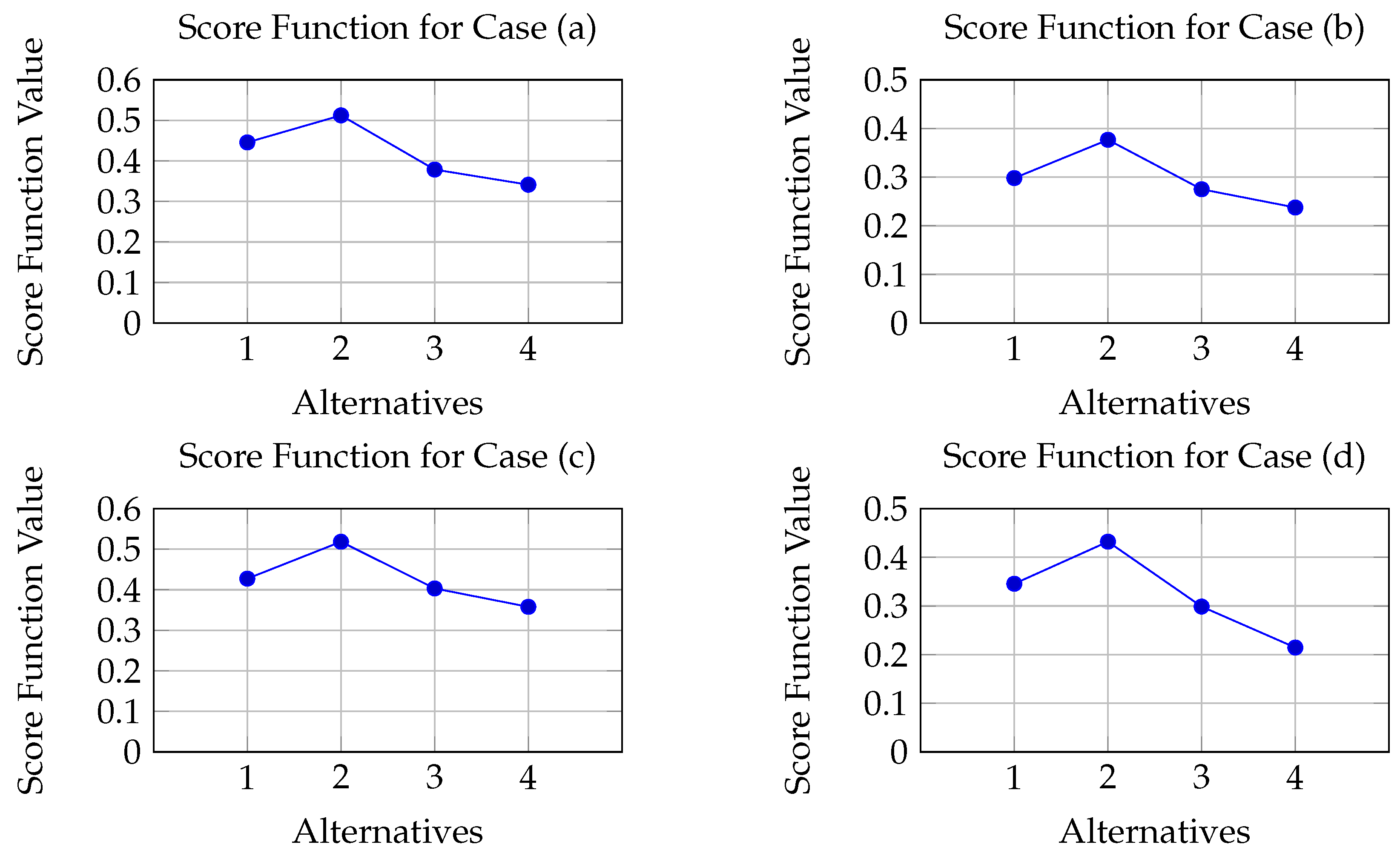
Step 5: The score function with respect to Case
(a) is shown in
Table 17.
The score function with respect to Case
(b) is shown in
Table 18.
The score function with respect to Case
(c) is shown in
Table 19.
The score function with respect to Case
(d) is shown in
Table 20.
Figure 2 shows the score function for Cases (
a–
d).
Step 6: The ranking result with respect to Case (a):
The ranking result with respect to Case (b):
The ranking result with respect to Case (c):
The ranking result with respect to Case (d):
Discussion
The supplied operators GCIFAAAGSCI and CIFAAAGSCI are employed in
Table 13,
Table 14,
Table 15 and
Table 16 of the study to provide the evaluations and ranks of various alternatives (where i = 1, 2, 3, 4). The constant conclusion over the following graphs shows that the option
is the ideal pick independent of the swings in overall evaluations and rankings for each alternative. Option
is the least preferred alternative, indicating the usefulness of the GCIFAAGGSCI and CIFAAGGSCI operators in completely analyzing the relevance of criteria combinations, their hierarchical structures, and the interrelations among these combinations. The alternative
outperforms
under the GCIFAAAGSCI operator primarily due to its consistently higher membership degrees and lower non-membership degrees across most evaluation criteria. This indicates a stronger overall performance with minimal hesitation and conflict in expert judgments. The GCIFAAAGSCI operator, by integrating the generalized circular intuitionistic fuzzy information with the Aczel–Alsina aggregation mechanism, effectively emphasizes criteria where
excels while sensitively penalizing weaker attributes. Consequently, the aggregated score of
surpasses that of
, reflecting its dominance in the decision-making context. This complete technique, which gives a global picture on DMs’ situations, allows operators to disassociate themselves from an incorrect measure-based CI. Unlike the CI, which may miss the extensive global interconnections between variants, the suggested approaches give a more complex and complete evaluation. Furthermore, the proposed technique offers a flexible strategy that fits the desires and aims of decision-makers via the inclusion of an element that establishes the HTN. This adaptability facilitates decision making, resulting in more dependable and informative outputs, unlike methods that rely primarily on mathematical t-norm procedures. The GCIFAAAGSCI and CIFAAGGSCI operators are useful in solving MCDM cases defined by ambiguity, as demonstrated in
Table 13,
Table 14,
Table 15 and
Table 16. This promotes better consistency and optimum decision making. The results exhibit low sensitivity to the Aczel–Alsina parameter
. As shown in the sensitivity analysis table, even as
varies from 1 to 5, the overall ranking of alternatives remains unchanged (
), indicating that the GCIFAAAGSCI operator is stable and robust across different
values.
7. Sensitivity Analysis
The sensitivity analysis reveals that the proposed GCIFAAAGSCI operator maintains stable rankings even when input weights are slightly varied, indicating high robustness and reliability. This consistency demonstrates the method’s resilience to minor fluctuations in expert preferences or data uncertainty. Consequently, it ensures dependable decision outcomes in practical multi-attribute environments.
7.1. Sensitivity to Aczel–Alsina Parameter
The robustness of the proposed GCIFAAAGSCI operator was further examined through a sensitivity analysis involving a variation of the Aczel–Alsina parameter
.
Table 21 summarizes the aggregated scores for all alternatives across a range of
values from 1 to 5. Despite noticeable changes in the numerical scores, the final rankings of the alternatives remain unchanged, maintaining the order
consistently. This invariant ranking pattern indicates that the proposed operator exhibits
low sensitivity to the parameter
, which is a desirable property for decision-making models operating under uncertainty. Specifically, as
increases, the operator tends to slightly magnify the separation between alternative scores; however, it does not disrupt the relative dominance among them. This reinforces the method’s capability to produce reliable and stable decision outcomes without requiring the meticulous tuning of operational parameters. Moreover, such stability is crucial in real-world applications where expert preferences or data characteristics may necessitate minor parameter adjustments. The ability of the GCIFAAAGSCI operator to preserve ranking order across these variations ensures its practical utility in domains like technology selection, healthcare policy evaluation, and investment decision analysis. The insensitivity to
also reflects theoretical soundness, as the underlying aggregation mechanism avoids any over-amplification of uncertainty or hesitation embedded in the fuzzy input information. Therefore, this analysis confirms that the proposed operator is not only computationally effective but also theoretically resilient to parameter perturbations, thereby enhancing its applicability and acceptance among decision analysts and practitioners.
7.2. Sensitivity to Input Weight Variation
To evaluate the robustness of the GCIFAAAGSCI operator under input perturbations, a sensitivity analysis was conducted by slightly varying the weights of the input attributes while keeping the Aczel–Alsina parameter fixed at
.
Table 22 shows the resulting aggregated scores and rankings for each variation. It is evident that although the scores change marginally, the final ranking order remains unaffected across all cases. This insensitivity to small fluctuations in attribute weights demonstrates the operator’s strong stability and reliability in practical scenarios. In many real-world decision environments, exact weight values may be difficult to determine due to incomplete or subjective judgments. The GCIFAAAGSCI operator’s ability to retain ranking consistency under such uncertainty makes it a practical choice for decision-making models. Furthermore, this behavior indicates that the method does not disproportionately amplify minor variations in the decision matrix, thereby ensuring that conclusions drawn from the decision model are both robust and interpretable.
8. Comparative Analysis
The author is conducting a comparative performance analysis between the proposed techniques and several existing techniques within different complex frameworks or environments. This analysis aims to offer insights into the merits and drawbacks of various methods, aiding in the selection of the most suitable approach for specific problems.
8.1. Comparison with Existing Methods of CIFSs
Comparative analysis is a basic decision-making method that entails weighing several options against predetermined criteria in order to choose the best option. That stage is crucial in MCDM situations since it makes it easier to use various developments, techniques, or aggregate ways to evaluate the possibilities. By evaluating the outcomes of various processes, one may obtain a better understanding of the reliability, stability, and utility of various decision strategies. To evaluate the advantages and disadvantages of different approaches and make sure they are in line with the goals of decision making, a comparative evaluation is used. By comparing the findings with those from other approaches and pointing out inconsistencies, it helps validate the results. When several approaches provide comparable evaluations or results, the decision-making process gains legitimacy. On the other hand, if there are notable disparities, further research is required to identify their reasons. We use a number of methods to make comparisons easier, such as relational parameter evaluation, measuring techniques, and visual aids. This approach works well in industries like technology, healthcare, and finance where there are many selection procedures and picking the right one is crucial. By offering a thorough assessment of possibilities from many angles, a comparison improves decision making.
An essential tool for determining how changes in input factors affect a decision’s result is vulnerability assessment. The ordering and decision-making procedures in MCDM are greatly influenced by factors including the consolidation of administrators, the allocated weights, and the desired values. Because even little changes to these factors might produce different results, it is crucial to assess the decision-making model’s robustness and durability. Sensitivity analysis helps decision-makers discover the most important aspects and evaluates the stability of the selected choice under several situations. In real-world situations where disparities may arise due to expert views, data uncertainties, and outside influences, this is very important. We investigate variable susceptibility in detail using various approaches such as Monte Carlo simulations, gradient-based methods, and one-at-a-time analysis. A robust selection system should exhibit minimal rank volatility whenever variables are altered within a reasonable range. If an option is very sensitive and changes significantly with little parameter changes, the framework must be continuously improved or the weight allocations must be reevaluated. Therefore, by ensuring that the chosen choice is optimal in a variety of situations, sensitivity testing enhances the reliability of decision-making processes.
The recommended approach is compared with a number of other previously used techniques in the present investigation.
[
24],
[
24],
[
24], and
[
24] are some of these tactics. We may have a better understanding of each strategy’s unique advantages and disadvantages as well as its success factors by contrasting them all. This information analysis may be used by researchers and decision-makers to identify the best approach for their requirements and preferences. Citations are also included for more study and comprehension of the concepts that underlie the tactics and strategy.
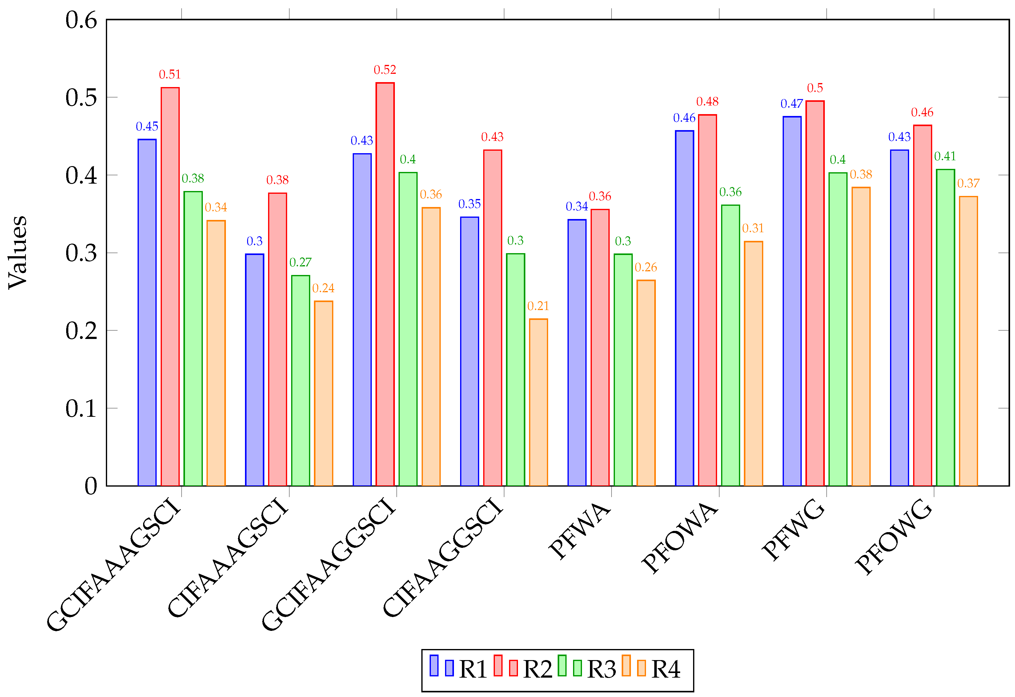
Table 23 and
Figure 3 presents the rankings obtained using the proposed methods, the namely
operator,
operator,
operator, and
CIFAAGGSCI operator which rank the alternatives as
. So, all proposed methods identify
as the best alternative.
However, operators like the operator, operator operator and produce a different ranking of with as the best alternative.
Furthermore, a detailed sensitivity analysis using techniques such as Monte Carlo simulation and one-at-a-time analysis reveals that the proposed methods maintain consistent rankings even when input parameters vary slightly. This robustness confirms their reliability in real-world applications where data uncertainty and expert disagreement are common.
8.2. Comparison with Existing Methods of PFSs
The recommended approach is compared with a number of other previously used techniques in the present investigation.
[
15],
[
15],
[
15], and
[
15] are some of these tactics. We may have a better understanding of each strategy’s unique advantages and disadvantages as well as its success factors by contrasting them all. This information analysis may be used by researchers and decision-makers to identify the best approach for their requirements and preferences. Citations are also included for more study and the comprehension of the concepts that underlie the tactics and strategy.
Table 24 and
Figure 4 presents the rankings obtained using the proposed methods, namely the
operator,
operator,
operator, and
CIFAAGGSCI operator, which rank the alternatives as
. So, all proposed methods identify
as the best alternative.
However, operators like the operator, operator operator and produce a different ranking of although they also identify as the best alternative. These observations confirm the proposed operators’ effectiveness in managing hesitancy and vagueness, which are prevalent in many real-world decision-making contexts.
8.3. Comparison with Existing Method of IFSs
The table’s comparison analysis provides insightful information about how well different aggregation operators handle alternate values. Researchers may find the aforementioned data to be a useful tool in choosing the best aggregation operator for their specific set of evaluation criteria. By providing opportunities for more study into the approaches associated with each operator, the citation references offered also contribute to better comprehension and decision-making processes.
The recommended approach is compared with a number of other previously used techniques in the present investigation:
[
9],
[
9],
[
9], and
[
9] are some of these tactics. We may have a better understanding of each strategy’s unique advantages and disadvantages as well as its success factors by contrasting them all. This information analysis may be used by researchers and decision-makers to identify the best approach for their requirements and preferences. Citations are also included for more study and comprehension of the concepts that underlie the tactics and strategy.
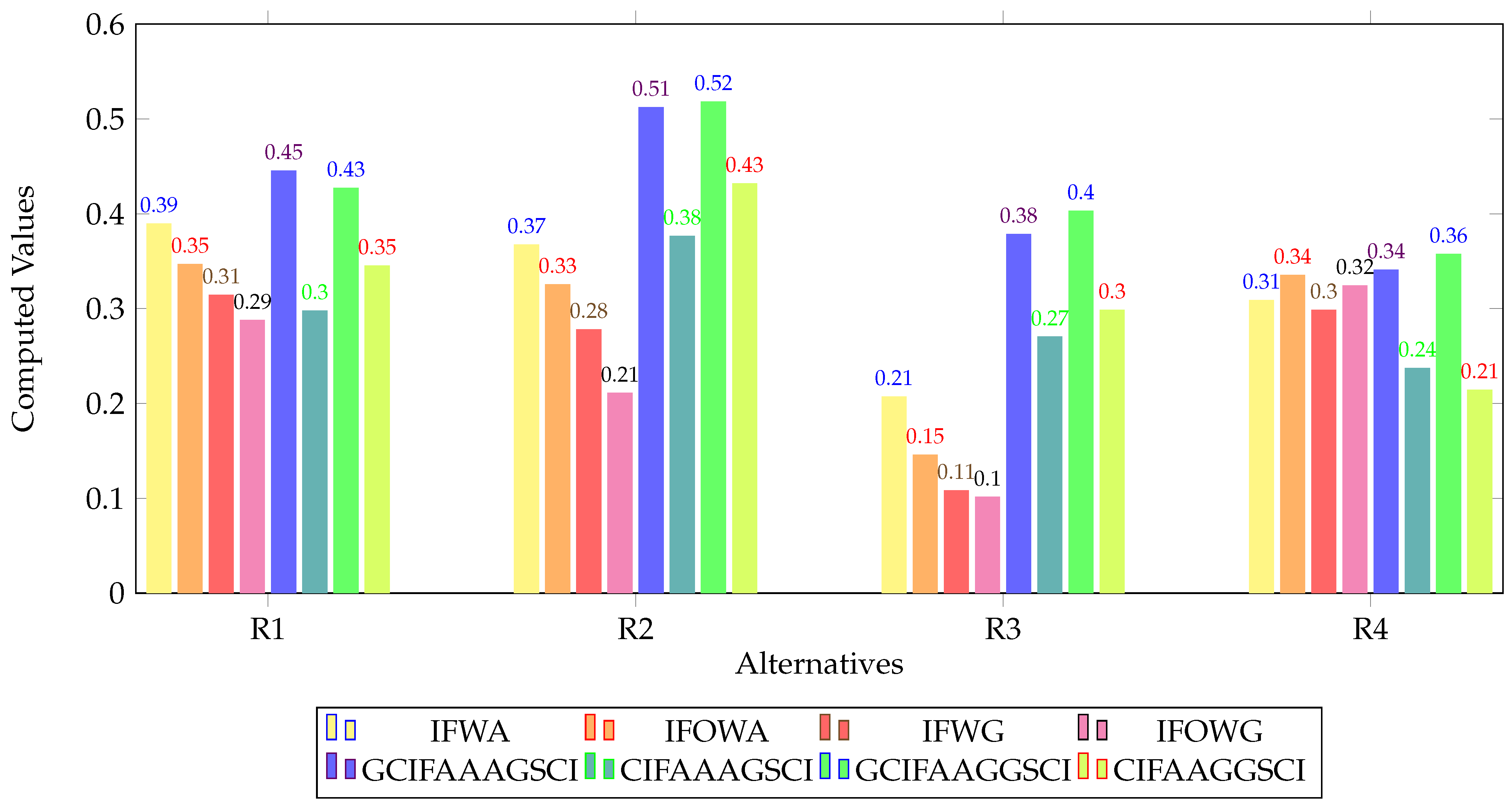
Table 25 and
Figure 5 presents the rankings obtained using the proposed methods, namely the
operator,
operator,
GCIFAAGGSCI operator, and
CIFAAGGSCI operator which rank the alternatives as
. So, all proposed methods identify
as the best alternative.
However, operators like the operator, operator operator and produce a different ranking of , although they also identify as the best alternative.
The comparative study of the table offers valuable insights regarding the efficiency of various aggregation operators when handling alternative values. The aforementioned data might be a valuable resource for researchers in selecting the most appropriate aggregation operator for their particular set of assessment criteria. The citation references provided also aid in improving understanding and decision-making processes by offering avenues for further research into the methodologies related to each operator.
8.4. Discussion
The comparative studies conducted across various fuzzy environments including CIFS, PFS, and IFS frameworks clearly demonstrate the superior performance of the proposed aggregation operators. These operators exhibit a high degree of robustness and consistency in decision outcomes, maintaining stable rankings even under varying input conditions. Such stability is particularly vital in real-world decision-making scenarios, where data uncertainty, incomplete information, and expert disagreement are common challenges. Additionally, the proposed methods show significantly lower sensitivity to parameter fluctuations compared to classical operators, thereby enhancing the overall reliability of the decision-making process. Another critical advantage lies in their ability to better incorporate expert judgment, making them well suited for complex, subjective evaluations. The practical applicability of these operators spans diverse fields, such as technology selection, healthcare policy planning, and financial investment analysis, where making accurate, interpretable, and justifiable decisions is crucial. These findings collectively underline both the theoretical strengths and the practical utility of the proposed methodology. Moreover, the included citation references offer readers the opportunity to delve deeper into the comparative strategies and computational mechanisms involved, thereby enriching their understanding of advanced fuzzy decision-making techniques.
9. Conclusions
In this study, we introduced two novel operators, GCIFAAAGSCI and GCIFAAGGSCI, which were designed to address MCDM challenges in CIF environments. These operators significantly enhance decision making by effectively managing uncertainty and criteria interactions, offering a systematic and structured approach that improves the effectiveness of decision-making processes. Through a detailed analysis, we demonstrated their distinctive features and advantages over traditional methods. The research presents a comprehensive solution to MCDM problems by leveraging these operators, which are specifically tailored to handle intricate decision scenarios.
The main contributions of this research include advancing the field of fuzzy decision making by integrating the Shapley Choquet integral with the Aczel–Alsina t-norm and t-conorm. These operators provide a more nuanced and flexible approach to aggregating information in CIF environments, which is crucial for real-world applications involving complex and uncertain data. The findings confirm that the proposed operators offer superior performance in handling uncertainty and interaction effects among criteria in MCDM problems. They allow for more precise and context-sensitive analyses, opening new possibilities for applying fuzzy logic in real-world scenarios where uncertainty and complexity are prevalent. The case study on bridge design selection demonstrates the practical applicability and effectiveness of these operators in producing consistent and reliable results, even in situations characterized by ambiguity and complexity. The sensitivity analysis further supports the robustness of the proposed methods, showing minimal ranking volatility when input parameters are varied within a reasonable range.
For future research, several directions can be explored to extend the findings of this study. First, the applicability of the GCIFAAGGSCI and GCIFAAAGSCI operators in different MCDM domains, such as healthcare, finance, and environmental management, could be investigated to assess their versatility and robustness. Second, further theoretical research into the mathematical properties of these operators would provide deeper insights into their behavior under various conditions. Third, integrating these operators with other decision support systems or hybrid models could offer new opportunities for improving decision-making frameworks in dynamic and uncertain environments. Additionally, exploring the potential of these operators in group decision-making scenarios and their extension to interval-valued intuitionistic fuzzy sets could be valuable avenues for future work. Finally, developing user-friendly software (Maple 2018) tools to implement these operators would facilitate their adoption in practical applications across various fields.


 ,
, 


