Abstract
The properties of light propagation underwater typically cause color distortion and reduced contrast in underwater images. In addition, complex underwater lighting conditions can result in issues such as non-uniform illumination, spotting, and noise. To address these challenges, we propose an innovative underwater-image enhancement (UIE) approach based on maximum information-channel compensation and edge-preserving filtering techniques. Specifically, we first develop a channel information transmission strategy grounded in maximum information preservation principles, utilizing the maximum information channel to improve the color fidelity of the input image. Next, we locally enhance the color-corrected image using guided filtering and generate a series of globally contrast-enhanced images by applying gamma transformations with varying parameter values. In the final stage, the enhanced image sequence is decomposed into low-frequency (LF) and high-frequency (HF) components via side-window filtering. For the HF component, a weight map is constructed by calculating the difference between the current exposedness and the optimum exposure. For the LF component, we derive a comprehensive feature map by integrating the brightness map, saturation map, and saliency map, thereby accurately assessing the quality of degraded regions in a manner that aligns with the symmetry principle inherent in human vision. Ultimately, we combine the LF and HF components through a weighted summation process, resulting in a high-quality underwater image. Experimental results demonstrate that our method effectively achieves both color restoration and contrast enhancement, outperforming several State-of-the-Art UIE techniques across multiple datasets.
1. Introduction
Since the beginning of the 21st century, the increasing competition for land and resources has made the protection and sustainable management of marine resources a strategic priority for the international community. Among them, underwater images are a critical medium of ocean information and play an irreplaceable role in the performance of ocean detection equipment. However, the distinct optical properties of underwater environments often lead to technical challenges such as color casts, blurred textures, and low contrast. These issues severely hinder the accurate extraction and analysis of image information. Consequently, the development of effective UIE techniques has become a pressing necessity.
To address the challenges in UIE, researchers have extensively investigated the mechanisms of underwater imaging and developed advanced image degradation models. At present, the existing UIE methods can be divided into three categories: physical model-based methods, non-physical model-based methods, and deep learning methods [1,2,3].
Physical model-based approach: This method mainly focuses on restoring underwater images by estimating model parameters and reversing the degradation process. In 2006, Trucco et al. proposed a UIE based on the Jaffe–McGlamery model [4] for the first time, but it performed poorly in color correction. Subsequently, the dark channel prior (DCP) method developed by He et al. [5] was introduced into the underwater domain. This method effectively corrects color casts owing to its superior dehazing capability, but its applicability is constrained by water’s selective light absorption. To address this limitation, researchers have developed various DCP enhancements, including a denoising algorithm [6], contrast-enhancement techniques [7], integrated color-correction approaches [8], and non-local prior-based restoration methods [9]. Although these adjustments have improved the quality of the image, several challenges persist, including heavy reliance on priors, noise amplification, and limited dynamic adaptability. In recent years, Zhuang et al. developed a retinal variation model inspired by the hyper-Laplacian reflection prior [10], but its effectiveness may decrease under low-light or high-turbidity conditions. The same limitation also exists in the optimized transmission map estimation method proposed by Hou et al. [11]. In 2024, Li et al. proposed a combination of adaptive optimization and particle swarm optimization algorithms [12], but its generalization is insufficient. Liang et al. [13] adopted a distinct strategy of transmittance minimization for contrast enhancement, but it introduced localized brightness inconsistencies. Until recently, the adaptive color-correction framework proposed by Zhang et al. [14] and the variation model developed by Yu et al. [15] have emerged as significant advances, demonstrating notable improvements in both color naturalness and algorithmic stability. In summary, the underwater-imaging mathematical models used in this kind of method are often too idealized, with problems such as insufficient robustness, limited flexibility, and high time costs for solving model parameters, which seriously limit their practical applications.
Non-physical model-based approach: The approach enhances underwater-image quality by performing pixel-wise value adjustments to improve color fidelity and visual clarity. Currently, the common non-physical model-based methods mainly include histogram-based methods, Retinex-based methods, and fusion-based methods. The histogram-based method enhances contrast by reallocating pixel values in the image. The Rayleigh histogram stretching introduced by Ghani et al. [16] significantly improves image quality but has been criticized due to noise amplification in low grayscale areas and limitations of fixed models. To address this issue, the adaptive global stretching algorithm [17] developed by Huang et al. cleverly resolves this contradiction through a dynamic parameter mechanism. Peng et al. proposed a staged processing method [18], which first restores colors through physical modeling, and then applies histogram equalization to ultimately achieve a more balanced enhancement effect. The Retinex-based method addresses color distortion by emulating the human visual system’s mechanisms for perceiving light and color. Fu et al. were the first to develop UIE based on Retinex [19], solving the typical problem of aquatic-image degradation effectively. Building upon this foundation, Ghani et al. [20] enhanced both chromatic accuracy and contrast through innovative integration of Rayleigh distribution principles. However, there was a slight over-enhancement phenomenon. To overcome this limitation, Zhuang et al. proposed the Bayesian Retinex algorithm [21], which ultimately achieved good results in color fidelity and scene adaptability. The fusion-based method integrates the advantages of different enhancement algorithms to achieve more natural underwater images. In 2018, Ancuti et al. developed Color Balance Fusion (CBF) [22], which effectively suppressed oversaturation artifacts. In order to further improve the visibility of underwater images, Zhang et al. [23] proposed a multi-channel convolutional multi-scale Retinex model with a color-restoration function. At the same time, Zhang et al. [24] adopted different methods and proposed a hybrid optimization approach by integrating multiple enhancement techniques. Hu et al. coupled color correction with brightness fusion [25] to make color more realistic. It is worth noting that Zhang’s team has been continuously cultivating in this field and has proposed the UIE based on weighted wavelet fusion [26], as well as the more advanced wavelet decomposition based on dominant contrast fusion [27]. The latter effectively integrates the advantageous features of various enhanced images, ultimately achieving better performance. Generally speaking, UIE that relies on non-physical models aims to align the image more closely with subjective visual perception. However, these methods often overlook the fundamental principles of underwater imaging, which may result in distortion of the final output.
Deep learning-based approach: Currently, deep learning-based methods can be divided into convolutional neural network (CNN) and generative adversarial network (GAN) [28]. This type of method learns the complex color-distribution characteristics of underwater images through massive data and has become a research hotspot in this field [29,30], demonstrating excellent performance in image-enhancement tasks [31,32,33,34].
CNN is widely used in UIE due to its ability to extract hierarchical features. In 2018, Lu et al. pioneered the use of deep convolutional neural networks [35] to solve the scattering problem of low-light underwater images, opening up a new direction in this field. In 2020, Li et al. made significant breakthroughs on this basis and proposed an underwater enhanced CNN based on scene statistics [36]. In the same year, Jiang et al. [30] further optimized the network architecture and designed a lightweight cascaded network to achieve efficient UIE processing. Yuan et al. [37] integrated multi-level wavelet transform and Runge Kutta module to develop a refined sub network. NAIK et al. [38] proposed a shallow neural network algorithm that can achieve advanced technology with only a small number of parameters. Ma et al. developed a wavelet-based dual-stream network [39] and achieved excellent performance. Recently, Tun et al. [40] solved the gradient-vanishing problem by introducing skip connections and integrating parameter-free attention modules into convolutional blocks. At the same time, Zhang et al. enhanced multi-scale detail-processing capabilities by using intrinsic supervision and ASISF modules [41]. Recently, Tolie et al. [42] combined convolutional neural networks with attention mechanisms to further improve the quality of UIE. GAN is a deep learning model that synthesizes realistic data through adversarial training of generators and discriminators. Anwar et al. [43] pioneered the application of generative adversarial networks to UIE in 2018, marking a paradigm shift in the field’s methodology. Subsequently, Guo et al. [44] proposed a multi-scale dense generative network. To achieve superior enhancement performance, Liu et al. [45] designed a target-driven dual-GAN architecture, but with increased complexity. In the same year, Chao et al. [46] combined multi-color spatial features with GAN framework, improving the quality of UIE significantly. Wang et al. [47] reduced inter-domain and intra-domain differences from the perspective of domain adaptation. In the latest progress, Zhou et al. [29] introduced a hybrid contrastive-learning strategy, which not only improves the enhancement performance but also significantly enhances the model’s generalization ability. In recent years, the application of symmetry theory in UIE has shown great potential. A noteworthy example is the PIC-GAN model [48], which includes a symmetric multi-level feature-extraction network based on the U-Net structure. This symmetrical design ensures a balanced flow of spatial and semantic information, improving the network’s adaptability to complex underwater scenes. However, both CNN and GAN require large-scale, high-quality datasets to effectively generalize, thus severely limiting their development.
The performance of methods based on a non-physical model is usually superior to the performance of the other two methods, as they are not limited by a physical model and real underwater-image data. Therefore, we focus on studying UIE based on a non-physical model along this technological route. Among non-physical model-based methods, the CBF method [22] achieved outstanding performance for UIE. This method utilizes different strategies to enhance color-correction results and integrates useful information from each enhanced result using a Laplacian pyramid. However, the enhancement strategies in the CBF method demonstrate limited robustness and scenario-dependent performance, particularly when applied to diverse underwater conditions. In response to these issues, this article proposes a novel UIE method aimed at achieving more efficient and robust image-enhancement effects. Initially, we developed a channel information-transformation mechanism grounded in maximum information-preservation principles. This mechanism employs the information transfer channel to perform color rectification on input images. Subsequently, we implement local enhancement of the color-adjusted images through guided filtering. At the same time, we apply varying gamma values to optimize the global contrast of the images. Ultimately, the processed image sequence undergoes decomposition into LF and HF components via side-window filtering, with customized fusion rules designed according to component characteristics to achieve high-quality underwater imaging.
Our primary contributions can be encapsulated in the following four key points:
- (1)
- We have developed a novel approach for UIE that demonstrates both efficiency and robustness. Numerous experiments have shown that our method is comparable to the latest UIE methods in qualitative and quantitative comparison, application testing, runtime, and generalization testing.
- (2)
- A maximum information channel for color correction is proposed. Specifically, we derive a reference channel from the principle of maximum information retention and utilize this reference channel to color-correct the input image. Compared with conventional techniques, our method eliminates the need for supplementary reference images while maintaining both efficiency and reliability.
- (3)
- An effective strategy for enhancing image contrast is proposed. In detail, we employ guided filtering to achieve local detail enhancement of color-corrected images while utilizing gamma transformation with varying parameter values to achieve a global contrast-enhancement effect.
- (4)
- An image-fusion technique based on side-window filtering is proposed. We utilize side-window filtering to decompose the pre-enhanced image sequence into LF and HF components. These components are then integrated using different rules to produce high-quality underwater images.
2. Preliminaries
2.1. Atmospheric Scattering Model
The quality deterioration observed in both atmospheric haze images and underwater photographs primarily results from light absorption and scattering phenomena within their respective transmission media. Therefore, the atmospheric scattering model [49], which describes the optical imaging process on foggy days, can often be adapted to represent the underwater optical imaging process under certain conditions roughly. Unlike atmospheric haze images, underwater light transmission exhibits wavelength-dependent attenuation, leading to varying degrees of color distortion in underwater images. Additionally, light scattering in water significantly degrades image quality. The Jaffe–McGlamery model [50] proposes that the direct incident component refers to the portion of light reflected from underwater objects that reaches the camera after undergoing attenuation through the aquatic medium. The forward-scattering component represents the small-angle scattering of reflected light from underwater objects before entering the camera, which causes the halo phenomenon in underwater images. The backscattering component passing through the underwater medium before entering the camera often causes blurring and contrast degradation in underwater images.
Figure 1 shows an underwater-imaging model. When viewed from left to right, the vertical coordinate of right 1 represents the light intensity (%), and the vertical coordinate of right 2 represents the light-propagation distance (m). In addition, different colors represent light of different wavelengths. As the water depth increases, the longest wavelength (red light) disappears first. Blue light has a shorter wavelength and stronger penetration. This is one of the main reasons why underwater images often exhibit blue–green tones.
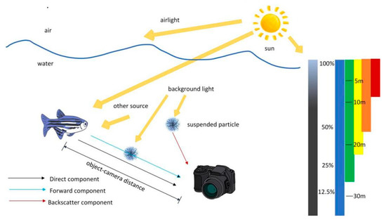
Figure 1.
Underwater optical imaging model.
Following the Jaffe–McGlamery model [50], the simplified atmospheric scattering model can be modeled using Equation (1):
In Equation (1), is the pixel point coordinates; represents channel of the observed image; represent the red, green, and blue channels of the color image; represents the raw image; is the global background scattered light; and transmission map is the medium transmittance of channel . The simplified underwater camera model (1) resembles Koschmieder’s atmospheric light-propagation model [51] but does not account for the strong wavelength dependence of attenuation in underwater environments, which is why our approach avoids explicit inversion of the light-propagation model.
2.2. Side-Window Filtering
In practical image-processing applications, achieving a balance between noise reduction and edge preservation has been a long-standing challenge. To meet these challenges, researchers have proposed some edge-preserving filtering algorithms with superior performance, such as bilateral filtering [52], mutual structure joint filtering [53], and curvature filtering [54]. When dealing with edge areas, these algorithms typically place the pending pixel at the center of the operation window, potentially resulting in blurred edges. To solve this problem, H. Yin et al. considered the symmetry of images and proposed an effective filtering method in 2019—side-window filtering (SWF) [55]. SWF reduces noise and preserves edges on the target image. SWF involves placing the pixels to be processed on the edges of eight windows: top, bottom, left, right, northeast, southeast, northwest, and southwest. When filtering, the pixels to be processed are only linearly combined with pixels in a certain direction of the window for calculation. Considering the requirements of edge preservation and minimizing the spacing between input and output at the edges, the filter will select a certain window containing the target pixel. It prevents the selection of regions with noise as the window. This approach helps cut down noise interference, achieving noise reduction while preserving edges.
Figure 2 shows the window for side-window filtering. Assuming that the target pixel is , let the filter kernel that is applied to the filter window be . The result of SWF [55] is given in Equation (3):
where is the filtered result; denotes the pixel value of input image at location ; is the radius of the filter window; denotes the position of the target pixel, ; and represents the direction of the filter window. By utilizing Equations (2) and (3), we were able to minimize the distance between the input and the output at the edge. The filtered result can approximate the input as closely as possible at the edge. Consequently, SWF has a strong ability to maintain the edge. Figure 2 shows the windows for SWF. In Figure 2, pixel is in the side-window position when , and it is in the top corner position when , and denotes the eight window orientations.
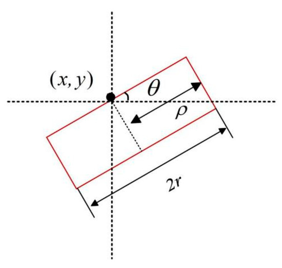
Figure 2.
Windows for side-window filtering.
3. Proposed Method
First, we propose a channel information-transformation mechanism based on maximum information-preservation principles, utilizing the maximum information channel to perform color correction on input images. Next, we apply guided filtering to locally enhance the color-adjusted images, followed by gamma transformation with varying parameters to generate a globally contrast-optimized image sequence. Finally, the enhanced image sequence is decomposed into LF and HF components via side-window filtering, with distinct fusion rules applied to integrate them into a high-quality underwater image. The overall workflow is illustrated in Figure 3.
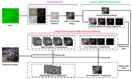
Figure 3.
Flowchart of the proposed method.
3.1. Color Restoration of Underwater Images Based on Maximum Information Transfer
Recently, statistical-based color correction [10] and segment-based color correction [56] have performed well in UIE. However, these corrections introduce some color cast, resulting in unrealistic image colors. To solve these problems, we propose a channel information-transformation mechanism grounded in maximum information-preservation principles, employing the maximum information channel for input-image color correction. In Figure 4, we show the flowchart of maximum information transfer for color correction. This section comprises two essential steps: defining reference channels and executing color compensation.
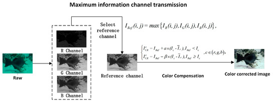
Figure 4.
Flowchart of underwater-image color correction based on maximum information transfer.
The Gray-World Hypothesis [57] proposes that the three primary color channels maintain similar mean gray values and histogram distributions. However, each channel of an underwater image has a different degree of attenuation. Thus, there will be a situation where color correction will be performed according to the grayscale-world hypothesis. To solve this problem, we need to determine the specific attenuation value for each channel. First, we separate the raw image into red, green, and blue channels and compute their pixel values, respectively. In Figure 4, the image with the highest pixel values among the three channels retains the most information, that is, the least image attenuation. Based on the above findings, we propose the principle of maximum information retention. According to this principle, the channel with the highest signal fidelity is selected as the reference channel to compensate for the color distortion in the other two severely attenuated channels. For a raw image, , the reference channel is defined as , and its calculation formula is provided in Equation (4):
By leveraging Equation (4), we can obtain the channel with the richest information content, so it can be used as a reference channel for the attenuation-channel compensation. Subsequently, the other two color channels are segmented and adjusted based on the reference channel, as illustrated in Equation (5):
In Equation (5), and these values serve as the gain adjustment coefficients for their respective channel components; , , and are the maximum, minimum, and average values of channel c; and represents the color-restoration image. We can see from Equation (5) that when , the intensity range of each color channel is normalized to the interval through linear stretching. Analogously, when , each channel’s gray level distribution is scaled to span the range using value stretching. Ultimately, the color-compensation procedure can be mathematically expressed using Equation (6):
By using Equation (6), we can adaptively compensate for the attenuation channels and stretch the pixel distribution. This color-correction operation effectively mitigates the color distortion present in underwater images. Figure 5 shows the histograms of pixel distributions for the three channels before and after color correction. The images are shown above the histograms. As can be seen in Figure 5, after implementing our color-restoration method, the curve distributions of the three channels are approximately consistent, and the image is more realistic and natural. However, the obtained image still faces the issues of insufficient contrast and blurry detail enhancement. Therefore, in the next section, we employ guided filtering and gamma correction to enhance the local and global contrasts of the image, respectively.
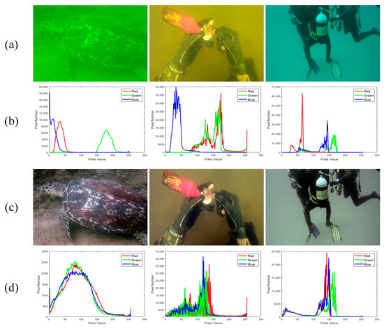
Figure 5.
Histograms of pixel distributions corresponding to each of the three channels before and after color restoration. (a) Raw image, (b) raw distribution histogram, (c) post-correction image, and (d) post-correction distribution histogram.
3.2. Acquisition of Global Contrast and Detailed Image Enhancement
As demonstrated in the previous section, the proposed color-restoration method achieves quantitatively validated improvements. However, as the depth of the water increases, optical absorption becomes more pronounced. This depth-dependent attenuation disproportionately affects red and green wavelengths, leading to significant spectral imbalance. Although color-compensation algorithms can mitigate these effects, residual information loss persists throughout the image, with the most severe degradation occurring in deeper water layers. To address this problem, we obtain a globally enhanced image sequence by applying gamma transformation to the color-corrected image using different parameters. Although gamma correction is effective in improving the global contrast of an image, some details may still be lost due to image exposure or underexposure. Thus, we simultaneously sharpen the color-corrected image by employing unsharp masking based on guided filtering to obtain our other input image, that is, enhancement of the image by blending with blurred images.
3.2.1. Acquisition of Exposure Image Sequence via Gamma-Corrected Transformation
We introduced gamma correction to further improve the image quality and solve the problems that remain after color correction. Gamma correction [22,58] can change the brightness and contrast of the image, which is given in Equation (7):
In Equation (7), is the gamma-corrected result; is the pixel value of the color-restoration image at location ; is a constant, which regulates the overall luminance; and is the gamma value, which governs the luminance contrast properties of the image. When , the darker image components are intensified, and the brighter portions are reduced, whereas when , the bright parts are enhanced, and the dark parts are compressed. Figure 6 shows the gamma-correction results using different parameters. It can be seen from Figure 6 that gamma transformation effectively improves the visibility of local details in low-light areas and the clarity of occluded areas. This method can effectively restore some lost details, especially in areas with deep water. Therefore, we set different values of to obtain a globally enhanced sequence, , by using Equation (7).
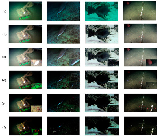
Figure 6.
Sequence of gamma-corrected exposure images. (a) Raw image; (b) color-corrected image; (c) exposure image processed with ; (d) exposure image processed with ; (e) exposure image processed with ; and (f) exposure image processed with .
3.2.2. Obtaining Detail-Enhanced Images Based on Guided Filter
Image sharpening is a common image-processing technique designed to enhance the details and edges of an image to make it look sharper. A common technique used in the sharpening process is unsharp masking [20,58], which implements sharpening effects by integrating the difference map between the input image and its Gaussian-smoothed equivalent. The typical formula for image sharpening is given by Equation (8):
where represents the detail-enhanced result, denotes the result of the image processed by a Gaussian filter, and parameter regulates the degree of sharpening intensity applied to the image. This sharpening process significantly improves image-appearance detail, particularly within the HF components of the image spectrum. However, unsharp masking by using Equation (8) has some problems in practical application, mainly in regard to two aspects. First, if the parameter is too small, the sharpening effect will be insufficient, and the image details will not be effectively enhanced. On the contrary, if the is too large, the image in the highlighted region will be too bright, and the shadow region will be too dark, resulting in color distortion. In addition, unsharp masking also tends to amplify HF noise, particularly at the edges of the image or in areas with more complex textures. The most significant issue is the “gradient reversal” artifact at the edges of the image. Gaussian filtering often cannot smooth this out, resulting in unnatural halo effects in the image.
For the first problem, to avoid selecting a parameter that is too large or too small, resulting in poor image enhancement, we adaptively select the value based on the image brightness. The parameter is given by Equation (9):
where is the average brightness of , which is a good indicator of the image-brightness appearance. It can be seen from Equation (9) that the value of parameter is correlated with the average luminance of the image. Therefore, the selection of has strong adaptability.
The guided filtering [59] is a non-local linear model that enhances image detail more accurately by leveraging the non-local similarity of the guided image. Unlike the Gaussian filter, the guided filter avoids the amplification of noise, as well as the generation of edge artifacts, by guiding the transfer of information from similar regions in the image. This method allows the guided filter to preserve finer image details during enhancement while effectively suppressing high-frequency noise interference. The optimized sharpening algorithm is formally represented by Equation (10):
In Equation (10), is the result of the image processed using the guided filter. The sharpening method defined in Equation (10) boasts the advantage of necessitating no parameter tuning and demonstrates effectiveness in enhancing sharpness, as evidenced by the example in Figure 7.
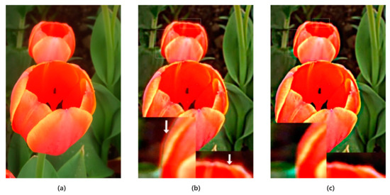
Figure 7.
Comparison of different enhancement results. (a) Raw image, (b) image enhanced using Gaussian filtering, and (c) image enhanced using guided filtering.
Figure 7 shows the image enhancement results using different filters. Compared with Figure 7c, the edge of Figure 7b exhibits obvious “gradient reversal” artifacts, especially in high-contrast areas. In Figure 7c, the sharpening effect of the image edges is smooth and natural, without a halo effect, and details are better preserved. Leveraging non-local image similarity as guidance, the guided filter simultaneously improves global image quality and local detail representation. This approach effectively eliminates the gradient-reversal artifacts inherent to Gaussian filtering while maintaining natural image appearance during detail enhancement. This indicates that the guided filter can effectively avoid the drawbacks of traditional methods, especially in edge regions, where it performs better. Following the preceding analysis, this paper specifically employs Equation (10) to enhance the details of color-corrected images.
The abovementioned process generates two vital components. One is a sequence of gamma-adjusted exposure images, which accentuate details in dark areas and refine image contrast. The other is an image that has been sharpened through guided filter processing, effectively boosting overall sharpness, especially evident in edge contours and fine textures. To obtain better enhancement results, we perform a multi-scale fusion of these two important inputs.
3.3. Multi-Scale Fusion
Single-scale fusion methods often have limitations in capturing comprehensive information, as they fail to fully consider the diverse details and context at various resolutions [27]. In contrast, multi-scale fusion methods are capable of extracting and integrating global and local features of an image at multiple scales, enabling clear and detailed image reconstruction. Thus, this paper employs a multi-scale approach to fuse different enhanced images. The method is divided into three main steps: extraction of LF and HF layers, construction of weight maps, and image fusion.
3.3.1. Enhanced Image Decomposition
LF components are designed to preserve the global structural information and object-boundary characteristics of an image. The choice of technique is particularly important when it comes to image-edge protection. Gaussian filtering, a classic and extensively used linear filtering technique, excels in enhancing image quality. It achieves this by eliminating random noise from the image through a convolution operation. However, this process inevitably blurs the boundaries, leading to the loss of edge information.
To overcome this limitation, SWF [55] has been developed as an advanced edge-preserving smoothing technique. Based on its demonstrated performance, we employ SWF to decompose the image into LF and HF components. The -th enhanced image, ( and ), undergoes sequential blurring operations to generate a base layer and multiple detail-enriched layers. Concretely, we set different values of to generate variably blurred images with differing intensity levels. The base layer, , is mathematically represented as Equation (11):
where , is the SWF function, is the window radius of the -th SWF, and is the decomposition level. Using Equation (11), we can obtain base layers with different blur levels by changing the radius value, . This processing pipeline facilitates the acquisition of an artifact-free base image while ensuring the preservation of crucial detail and edge information.
On the other hand, the HF image focuses on preserving information about details in small regions of the image that are crucial for object-recognition and image-understanding tasks. To achieve optimal results, we integrate the enhanced components with the base image through a fusion process that maintains both structural integrity and fine-detail preservation. Once the base layers are obtained, the detail layer is derived by subtracting the base layer of adjacent scales, which is given in Equation (12):
where is the HF image. This decomposition process is designed to divide each source image into a base layer, which encompasses the large-scale variations in intensity, and a series of detail layers, which capture the fine-scale details. After generating the LF image, , and the HF images, for -th enhanced image, , we construct weight maps for the image fusion process for effective detail preservation and structure synthesis.
3.3.2. Weighting-Map Construction
After acquiring LF and HF images, we need to construct weight maps for image fusion. Most weight map-construction methods utilize a unified feature map extracted from the source image to guide the fusion of LF and HF components [22,60]. Due to the different characteristics of LF and HF components, the fusion rules based on a unified feature map make it difficult to fully preserve the useful information of the source images, resulting in a limited fusion effect. In order to improve fusion performance, this article fully considers the different characteristics of LF and HF components, and constructs their respective feature maps. The fusion process employs an adaptive weighting scheme that dynamically adjusts according to regional exposure characteristics. Specifically, we construct pixel-wise weight maps based on the distinct exposure responses of LF and HF components to precisely control the multi-scale image fusion. HF images are concerned with the local details of the image. For the HF image, , we measure its exposure by calculating the average brightness of the local region to construct a weight map. The specific calculation process is as follows: for each pixel position in , we first use an average filter with to convolve the image block in to calculate its exposure feature, , and subsequently calculate the weights, , according to Equation (13):
where controls the steepness of the weight function. As is evident from Equation (13), when certain pixel values deviate significantly from the optimal exposure value of 0.5, their corresponding weights approach zero. Essentially, this weight function guides the pixel-wise fusion process to select the desired intensity levels, which are directly proportional to those in the HF images.
The LF image primarily captures the fundamental structure information in an image. Therefore, for the LF image, , we design three weight maps to assess brightness, color saturation, and saliency. These weight maps are derived from the local characteristics of each pixel to preserve important information.
The luminance weight map is used to evaluate the visibility of each pixel. We utilize the well-established property that more saturated colors result in elevated values in one or two of the color channels. Concretely, we determine the significance of each pixel in the image by calculating the deviation of its luminance value from its RGB channel. The formula for the brightness weight map, , is represented in Equation (14):
where , , , and are the red, green, blue, and luminance channels of . The brightness weight acts as an identifier of the degradation induced in the enhanced image. The disparity outlined in Equation (14) results in higher values for pixels with high contrast and are presumed to belong to the initial clear regions. On the contrary, in colorless and low-contrast image regions, the value of this indicator will be smaller. The fusion result derived from the brightness map often leads to a decrease in colorfulness. To mitigate these effects, our framework introduces two additional weight maps: a saturation map and a saliency map.
The saturation weight map is inspired by the general preference among humans for images that exhibit a high degree of saturation. We calculate the saturation value of each pixel and compare it with the maximum saturation to generate the corresponding weights. The formula for saturation weight map, , is given in Equation (15):
where and are the saturation and maximum saturation values of , and is the standard deviation. In Equation (15), pixels with decreased saturation are assigned smaller values, whereas those with the highest saturation receive larger values. As a result, this map guarantees that the initial saturated regions will be more accurately depicted in the fused output.
The saliency weight map is used to assess the degree of saliency of objects in an image. We use a saliency detection algorithm based on a biological vision model to calculate the contrast of each pixel with respect to its surrounding pixels. The formula for the saturation weight map, , is given in Equation (16):
where and are the central pixel and the surrounding pixel values of at location . The saliency map prevents the introduction of unwanted artifacts in the result image obtained through our method, as neighboring comparable values are assigned similarly on the map. Furthermore, the map we utilize emphasizes large regions and estimates consistent values across the entire salient areas. Thus, this weighting map is effective in identifying important regions in the image and ensures that these regions are given more attention during the fusion process.
By using these three weight maps, , , and , we can achieve finer control to ensure that important image features are preserved, and that artifacts and distortions are retained in the final result. Finally, we normalize these weight maps to ensure that their sum adds up to 1, resulting in overall brightness and color consistency of the image during the fusion process.
3.3.3. Integration Process
Once the estimation and normalization of the weight maps of all the enhanced images are completed, the enhanced images are merged into the fused image, , as shown in Equation (17):
In Equation (17), and are the normalized weight maps of the LF and the -th HF images of the -th enhanced image, and is the total number of enhanced images. By employing an independent fusion process at each scale level, we can minimize potential artifacts arising from the abrupt transitions in the weight maps. Through multi-scale decomposition-based fusion, we effectively integrate important information from different enhanced images and avoid the appearance of blending artifacts. This method not only preserves global structural information but also enhances local detail information, thereby generating more natural and realistic underwater images.
The proposed maximum information-channel correction and edge-preserving filtering process is presented in Algorithm 1.
| Algorithm 1. UIE based on maximum information-channel correction and edge-preserving filtering |
| Input: Original underwater image, . |
|
| Output: The enhanced underwater image, . |
4. Results
This section starts with an introduction to the setup of the experiment, and then it covers how we designed and implemented five sets of comparative tests to analyze. Due to the limited space, more experimental results can be found in the Supplementary Material.
4.1. Setup of the Experiment
Benchmark dataset: We used six widely used datasets for evaluation: BRUD [61], OD [62], RUIE [63], SAUD [2], UIDEF [64], and UIEB [49]. The BRUD dataset encompasses 100 images of varying ocean depths, such as depths less than 1 m, 1–2 m, and 2–3 m. The OD dataset captured 183 underwater images under dark conditions. The RUIE dataset is composed of nearly 7000 underwater images divided into three subsets: image color cast, visibility, and advanced detection. The SAUD dataset includes 100 real-world raw underwater images and 100 representative UIE algorithms that generate enhancement results. The UIDEF dataset consists of over 9000 images captured from real-world underwater scenarios, covering a wide array of underwater scenes and objects, such as coral reefs, fish schools, shipwrecks, etc. The UIEB dataset includes 950 real underwater images of different water quality, lighting conditions, and depths. Among them, 890 are enhanced images, and the remaining 60 are considered challenging image sets.
Evaluation metrics: Metric evaluation of underwater images can be classified into full-reference assessment and non-reference image-assessment metrics. In this study, we use Peak Signal-to-Noise Ratio (PSNR) [65] and Structural Similarity (SSIM) [66] for full reference evaluation. The higher these two assessment values are, the higher the similarity between the two images. In addition, we used the Underwater Image Quality Measure (UIQM) [67], Underwater Color Image Quality Evaluation (UCIQE) [68], Color Cast Factor (CCF) [69], and Average Gradient (AG) [70] for non-reference image-evaluation metrics, where higher values of these metrics represent better images. PSNR reflects the ratio of peak signal to average energy through maximum error and mean square error. SSIM measures similarity through brightness, contrast, and structure, with higher values representing better image quality. UIQM comprehensively considers the three dimensions of image color, clarity, and contrast and calculates the overall quality through weighted averaging. UCIQE is used to quantify non-uniform color cast, blur, and low-contrast issues in underwater images. CCF is mainly used to measure the degree of improvement in color richness of enhanced images. The AG index is an indicator that measures the clarity and detail preservation of an image.
Comparison methods: To scientifically and comprehensively verify the robustness and progressiveness of our methods, we selected nine advanced UIE methods, categorizing them into broad groups of recovery-based methods—BR [21] and HLRP [10]; and enhancement-based methods—CBF [22], CBLA [60], EUICCCLF [25], MCLLAC [70], PCDE [56], TEBCF [71], and WWPF [26]. BR and HLRP are based on Bayesian Retinex theory and the Retinex variation model, respectively. CBF, CBLA, EUICCCLF, MCLLAC, PCDE, and TEBCF are very advanced methods that use different enhancement strategies for UIE. WWPF is based on weighted wavelet visual perception fusion technology. These methods have their own characteristics and jointly promote the development of underwater image-processing technology.
Experimental environment and parameter settings: All the experiments are tested using MATLAB 2020a software on a 2024 Redmi Book Pro 16 computer configured with Ultra 5 3.1K 165Hz DCI-P3 32G 1T. With this experimental environment established, we now turn to the parameter settings of our method. Taking into account both the image-enhancement effect and computational efficiency, the primary parameter settings for our method are outlined as follows: the transformation coefficient is , and is fixed to 1 in Equation (7) to produce the globally enhanced sequence; the guided filter parameter is set to in Equation (10) to obtain the detail-enhanced image; the decomposition level is , and the radius is for the SWF-based multi-scale decomposition in Equation (11) to produce the LF image and HF images; the parameter is set to in Equation (13); the parameter is set to in Equation (15); and the size of patch is in Equation (16). Using the aforementioned parameters, the proposed method exhibits good enhancement effects across a diverse array of real-world underwater scenarios.
Experiment categories: To fully assess the effectiveness of the proposed method, we conducted five categories of experiments: qualitative comparison, quantitative comparison, application testing, complexity analysis, and limitation analysis.
4.2. Experimental Analyses
4.2.1. Qualitative Comparison
We used different methods to process images from six datasets: BRUD, OD, RUIE, SAUD, UIDEF, and UIEB. From these, we selected representative images for qualitative analysis. Figure 8, Figure 9 and Figure 10 show the results processed using the different methods.
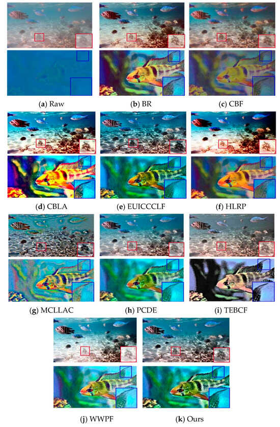
Figure 8.
Comparison of enhancement results of different UIE methods using the UIEB dataset.
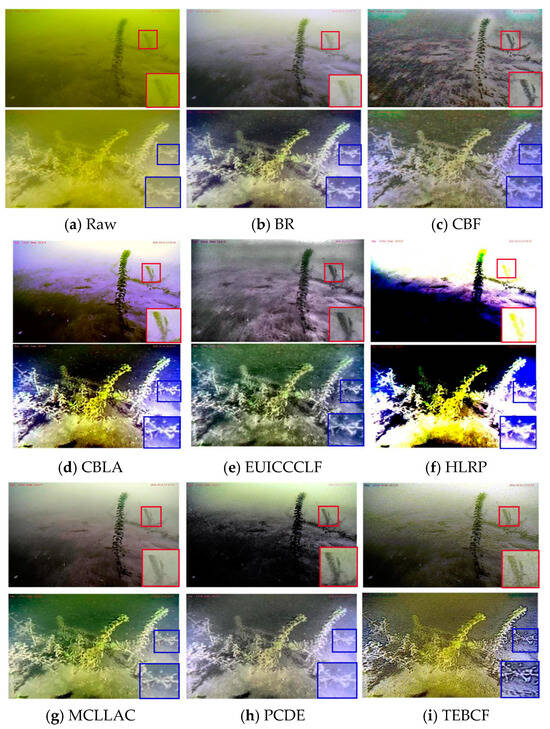
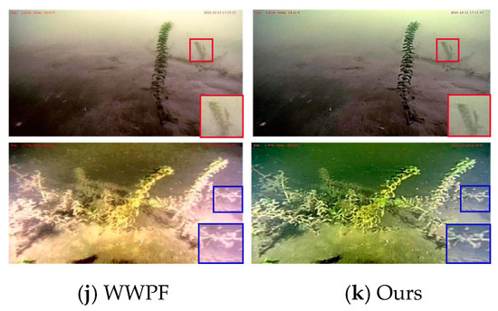
Figure 9.
Comparison of enhancement results of different UIE methods using the BRUD dataset.
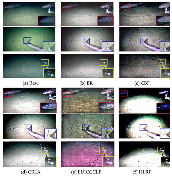
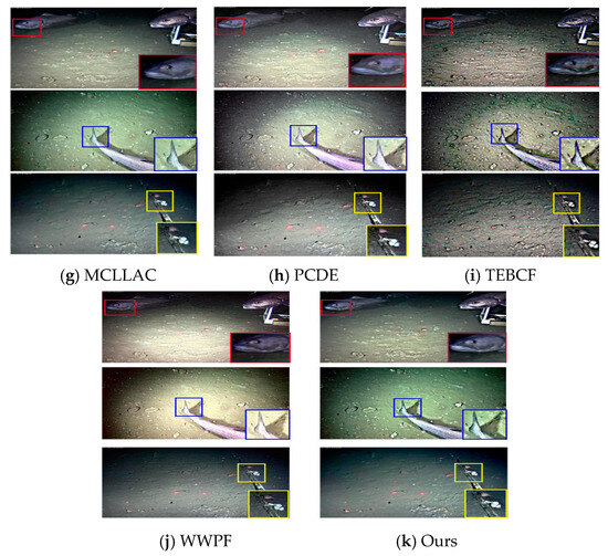
Figure 10.
Comparison of enhancement results of different UIE methods using the OD dataset.
Figure 8 shows two images selected from the UIEB dataset with blue distortion and image blur. The images obtained using our method have more natural and realistic colors, and they significantly enhance contrast. This improvement makes details such as fish and conch clearly visible, as shown in Figure 8k. In contrast, the PCDE and TEBCF methods are relatively poor at correcting natural colors and even introduce some noise, affecting visual quality seriously, as shown in Figure 8h,i. CBF eliminates color cast, but it performs poorly in contrast enhancement, as shown in Figure 8c. While CBLA and HLRP address color cast and improve global contrast effectively, these methods exhibit localized over-enhancement artifacts, leading to detail loss, as demonstrated in Figure 8d,f. Figure 8b shows that BR restores vivid and realistic colors to the scene and enhances contrast, but the overall brightness improvement is not as effective as that achieved using our method.
Figure 9 shows images with severe yellow distortion taken from different angles selected from the BRUD dataset. Figure 9b–f all have poor performance in terms of color correction. Due to excessive correction, the enhanced image even introduces purple tones, affecting the visual effect seriously, as shown in Figure 9d,f. Figure 9h,j show roughly removed color cast, but there is still insufficient contrast. Figure 9g shows that MCLLAC achieved natural colors and good contrast, similar to the effect produced by the proposed method.
Figure 10 shows the images selected from the OD dataset under low and uneven lighting conditions. Figure 10d,f demonstrate that CBLA and HLRP achieve luminance enhancement in challenging low-light conditions with non-uniform illumination, though with incomplete dynamic range recovery. The downside is that they may cause previously bright areas to become overly bright. Figure 10e shows that EUICCCLF increases image brightness without causing overexposure. However, its color reproduction effect is very poor, even introducing a hint of purple. Figure 10c achieves excellent contrast-enhancement but cannot truly restore the color of the scene. Compared with all methods, our method accurately reproduces the true color of the image while effectively suppressing the amplification effect caused by light-source interference, as shown in Figure 10k. Specifically, this method significantly improves the clarity of areas with insufficient brightness.
4.2.2. Quantitative Comparison
To objectively evaluate the effectiveness of our method, we selected UCIQE, UIQM, CCF, and AG as non-reference indicators for evaluation. In addition, due to the inclusion of reference images in the UIEB dataset, we added the full-reference metrics PSNR and SSIM. All the evaluated metrics exhibited a positive correlation with image quality, indicating that higher metric values corresponded to superior performance. Specifically, a higher UCIQE score signifies a more optimal balance among chroma, saturation, and contrast. Regarding UIQM, its value directly correlated with the overall quality of an image across three key dimensions: color, clarity, and contrast. For the CCF, a larger value denotes a more substantial enhancement in color richness. A higher AG value indicates that the enhanced image offers improved visual clarity and detail discernibility. In terms of PSNR, a higher score implies a closer match between the processed image and the ground-truth color. Meanwhile, SSIM measured the similarity in brightness, contrast, and structural elements between the processed image and the reference image; a larger SSIM value indicates a greater degree of similarity between them. Note that all existing underwater image-quality evaluation metrics are not sufficiently accurate: the scores of non-reference indicators cannot accurately reflect the visual quality of enhanced underwater images in some cases. Therefore, we need to take multiple indicators into comprehensive consideration instead of focusing on a single one. Table 1 shows the quantitative results of the six datasets we used. The top three results in each row are highlighted in bold with red, green, and blue, respectively. As shown in Table 1, compared with the raw image, our method has achieved significant improvement in objective measures. In almost all the evaluation indicators, it has obtained the highest score or ranked in the top three. For the OD dataset specifically, our method obtained the best or second-best results for all reference evaluation metrics. This is mainly because the study uses multiple gamma-correction algorithms with varying parameters, effectively reducing the impact of poor lighting in the OD dataset. The data presented in Table 1 further substantiate the superior performance of our approach in quantitative assessment.

Table 1.
Quantitative analysis of the six datasets (the three highest results in each row are highlighted in red, green, and blue, in that order).
4.2.3. Application Testing
Underwater-image feature-point matching: We analyzed our algorithm using the Harris corner detection method [72] and the SIFT feature-detection method [73].
Figure 11, Figure 12 and Figure 13 show the results of processing images with color distortion and those captured in dark scenes. Additionally, for the images with color distortion, we also compare our method with the deep learning-based enhancement approaches UWCNN [3] and Water-net [49].
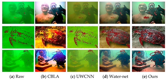
Figure 11.
Comparison of enhancement results of Harris detection of different UIEs for color-distorted image sets.
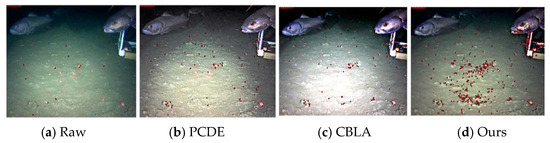
Figure 12.
Comparison of enhancement results of Harris detection of different UIEs for image groups in dark scenes.
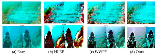
Figure 13.
Applying the SIFT operator for feature-point matching.
Figure 11 shows the processing performance of the Harris corner detector and three mainstream UIE methods. The results indicate that all the UIE methods significantly increase the number of corners compared to the raw image. It is worth noting that our method demonstrates superior feature-extraction capability, achieving the highest angular density among all compared techniques. In terms of spatial distribution, Figure 11b–d show relatively concentrated distributions, while the generated corner points in this study also have a wide spatial distribution, covering key structural areas of the image, as shown in Figure 11e. This characteristic indicates that our method effectively preserves richer global features while enhancing image contrast.
Figure 12 shows the image-processing results under dark scenes and uneven artificial lighting. The two methods in Figure 12b,c suffer from overexposure in bright areas, while the enhancement effect in dark areas is insufficient. Compared with conventional approaches, our method demonstrates superior performance in both feature point-detection quantity and spatial distribution. Notably, it achieves balanced feature distribution across various illumination regions, including shadow edges, mid-tone areas, and highlight zones. This wide distribution characteristic overcomes the shortcomings of traditional methods in local feature aggregation, providing more reliable input data for visual tasks such as underwater SLAM, long-term feature tracking, and 3D reconstruction.
Figure 13 shows the results of SIFT detection on images obtained using different methods. Figure 13a shows the raw degraded images, with only 533 and 13 feature matches detected for the top and bottom images, respectively. This demonstrates severe feature degradation due to underwater conditions. The number of matches increased after processing the image using HLRP and WWPF, as shown in Figure 13b,c. However, the most significant performance was achieved using our method, with 979 and 55 feature-point matches, respectively. These values are approximately 83.7% and 323% higher than those of the original image, as shown in Figure 13d. This result demonstrates the significant advantage of our algorithm in feature preservation.
4.2.4. Complexity Analysis
In this study, images of different sizes were used to demonstrate the computational complexity and advantages of our proposed method in terms of acceleration performance. To analyze the acceleration performance, we compared our method with other UIE methods using the RUIE and OD datasets. The size of images in the RUIE dataset is 400 × 300, and in the OD dataset, the size is 1280 × 720. Table 2 and Table 3 show the average running times of the different methods. The HLRP method demonstrates the highest efficiency, while the TEBCF method is the least efficient, mainly because the use of Contour Bougie morphology for image enhancement decreases the algorithm’s efficiency. Our method has a slightly lower average running time than the CBLA, EUICCCLF, and MCLLAC methods. However, the difference is not significant, and our method is relatively better based on qualitative and quantitative analysis and application testing.
Table 2.
Comparison of average running times of different underwater image-processing methods (image size = 400 × 300).
Table 3.
Comparison of average running times of different underwater image-processing methods (image size = 1280 × 720).
4.2.5. Limitation
We have shown that the quality of the raw image can impact the results. Figure 14 gives some examples of failure cases using our method. For images with significant loss of some details, the restoration effect is not ideal, and the clarity is insufficient, as shown in the second column of Figure 14. Enhancement of a low-brightness scene (the first column in Figure 14) results in color distortion, and the details of the enhanced image of a turbid scene (the third column in Figure 14) are unclear. In addition, information loss is severe in all channels of turbid and low-brightness images. Moreover, in highly turbid and blurry scenes, the edge texture information of the raw image is not clear. These issues render the global and detail-enhancement strategies ineffective, limiting the performance of our method. These remain major challenges for most current algorithms and may be solved by incorporating scene-depth information in future research.
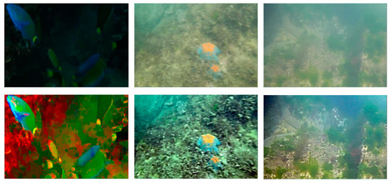
Figure 14.
Some examples of the limitations of our method. In the first row, from left to right, are the original images with low brightness, blurred images, and turbid scenes; the second row shows the results of image enhancement using our method.
5. Conclusions
In this study, we propose a UIE algorithm based on maximum information-channel correction and edge-preserving filtering. We first obtain a reference channel based on the principle of maximum information retention and use the reference channel to correct the color of the raw image. Unlike existing approaches, the proposed method achieves effective and robust performance without requiring reference images. Next, we use guided filtering to accomplish local enhancement of the color-corrected image and gamma transform with different parameter values for global contrast enhancement. Finally, we utilize side-window filtering to decompose the contrast-enhanced image sequence into LF and HF components and integrate the LF and HF components using different rules, thus generating high-quality underwater images. Numerous experiments have shown that our method is equally effective, or even better, than the latest UIE methods in terms of qualitative and quantitative comparisons, application testing, and runtime.
Although our method performs well, it is limited when it comes to enhancing some turbid and low-brightness scenes. In future work, we plan to optimize the algorithm to expand its application to more scenarios with image-enhancement requirements and continuously explore its application potential in different visual tasks, thus bringing more innovative possibilities to the field of computer vision.
Supplementary Materials
The following supporting information can be downloaded at: https://www.mdpi.com/article/10.3390/sym17050725/s1. Reference [74] is cited in the Supplementary Materials.
Author Contributions
Conceptualization, W.L. and P.Q.; Methodology, W.L., J.X., S.H., H.S. and P.Q.; Software, J.X., S.H. and Y.C.; Validation, J.X., Y.C. and X.Z.; Investigation, P.Q.; Writing—original draft, W.L., J.X., S.H., Y.C. and X.Z.; Writing—review & editing, W.L. and H.S.; Visualization, X.Z.; Funding acquisition, W.L. and P.Q. All authors have read and agreed to the published version of the manuscript.
Funding
This work was supported by the Key Project of Natural Science Research in Anhui Province (Grant No. 2022AH051750), in part by the Excellent Innovative Research Team of universities in Anhui Province (Grant No. 2023AH010056), and in part by the Fundamental Research Funds for the Tongling University (Grant No. 2022tlxyrc11).
Data Availability Statement
The raw data supporting the conclusions of this article will be made available by the authors, without undue reservation.
Acknowledgments
The authors would like to thank the editor and anonymous reviewers for their detailed review, valuable comments, and constructive suggestions.
Conflicts of Interest
The authors declare no conflicts of interest.
References
- Zhang, W.; Pan, X.; Xie, X.; Li, L.; Wang, Z.; Han, C. Color correction and adaptive contrast enhancement for underwater image enhancement. Comput. Electr. Eng. 2021, 91, 106981. [Google Scholar] [CrossRef]
- Jiang, Q.; Gu, Y.; Li, C.; Cong, R.; Shao, F. Underwater image enhancement quality evaluation: Benchmark dataset and objective metric. IEEE Trans. Circuits Syst. Video Technol. 2022, 32, 5959–5974. [Google Scholar] [CrossRef]
- Fu, X.; Cao, X. Underwater image enhancement with global-local networks and compressed-histogram equalization. Signal Process. Image Commun. 2020, 86, 115892. [Google Scholar] [CrossRef]
- Trucco, E.; Olmos-Antillon, A.T. Self-tuning underwater image restoration. IEEE J. Ocean. Eng. 2006, 31, 511–519. [Google Scholar] [CrossRef]
- He, K.; Sun, J.; Tang, X. Single image haze removal using dark channel prior. In Proceedings of the 2009 IEEE Conference on Computer Vision and Pattern Recognition, Miami, FL, USA, 20–25 June 2009; pp. 1956–1963. [Google Scholar]
- Chiang, J.Y.; Chen, Y.-C. Underwater image enhancement by wavelength compensation and dehazing. IEEE Trans. Image Process. 2012, 21, 1756–1769. [Google Scholar] [CrossRef] [PubMed]
- Liu, H.; Chau, L.-P. Underwater image restoration based on contrast enhancement. In Proceedings of the IEEE International Conference on Digital Signal Processing, Beijing, China, 16–18 October 2016; pp. 584–588. [Google Scholar]
- Li, C.; Guo, J.; Guo, C.; Cong, R.; Gong, J. A hybrid method for underwater image correction. Pattern Recognit. Lett. 2017, 94, 62–67. [Google Scholar] [CrossRef]
- Wang, Y.; Liu, H.; Chau, L.-P. Single underwater image restoration using adaptive attenuation-curve prior. IEEE Trans. Circuits Syst. I Regul. Pap. 2018, 65, 992–1002. [Google Scholar] [CrossRef]
- Zhuang, P.; Wu, J.; Porikli, F.; Li, C. Underwater image enhancement with hyper-laplacian reflectance priors. IEEE Trans. Image Process. 2022, 31, 5442–5455. [Google Scholar] [CrossRef]
- Hou, G.; Li, N.; Zhuang, P.; Li, K.; Sun, H.; Li, C. Non-uniform illumination underwater image restoration via illumination channel sparsity prior. IEEE Trans. Circuits Syst. Video Technol. 2024, 34, 799–814. [Google Scholar] [CrossRef]
- Li, Y.; Zhang, J.; Chen, Y.; Li, Y.; Tang, H.; Fu, X. Underwater image restoration via spatially adaptive polarization imaging and color correction. Knowl.-Based Syst. 2024, 305, 112651. [Google Scholar] [CrossRef]
- Liang, Z.; Zhang, W.; Ruan, R.; Zhuang, P.; Xie, X.; Li, C. Underwater image quality improvement via color. IEEE Trans. Circuits Syst. Video Technol. 2024, 34, 1726–1742. [Google Scholar] [CrossRef]
- Zhang, J.; Yu, Q.; Hou, G. Underwater image restoration via adaptive color correction and dehazing. Appl. Opt. 2024, 63, 2728–2736. [Google Scholar] [CrossRef]
- Yu, Q.; Hou, G.; Zhang, W.; Huang, B.; Pan, Z. Contour and texture preservation underwater image restoration via Low-rank regularizations. Expert Syst. Appl. 2025, 262, 125549. [Google Scholar] [CrossRef]
- Ghani, A.S.A.; Isa, N.A.M. Underwater image quality enhancement through Rayleigh-stretching and averaging image planes. Int. J. Nav. Archit. Ocean. Eng. 2014, 6, 840–866. [Google Scholar] [CrossRef]
- Huang, D.; Wang, Y.; Song, W.; Sequeira, J.; Mavromatis, S. Shallow-water image enhancement using relative global histogram stretching based on adaptive parameter acquisition. In MultiMedia Modeling; Springer International Publishing: Cham, Switzerland, 2018; Volume 10704, pp. 453–465. [Google Scholar]
- Peng, Y.-T.; Chen, Y.-R.; Chen, Z.; Wang, J.-H.; Huang, S.-C. Underwater image enhancement based on histogram-equalization approximation using physics-based dichromatic modeling. Sensors 2022, 22, 2168. [Google Scholar] [CrossRef] [PubMed]
- Fu, X.; Zhuang, P.; Huang, Y.; Liao, Y.; Zhang, X.-P.; Ding, X. A retinex-based enhancing approach for single underwater image. In Proceedings of the 2014 IEEE International Conference on Image Processing (ICIP), Paris, France, 27–30 October 2014; pp. 4572–4576. [Google Scholar] [CrossRef]
- Ghani, A.S.A.; Isa, N.A.M. Enhancement of low quality underwater image through integrated color model and local contrast correction. Appl. Soft Comput. 2015, 37, 332–344. [Google Scholar] [CrossRef]
- Zhuang, P.; Li, C.; Wu, J. Bayesian retinex underwater image enhancement. Eng. Appl. Artif. Intell. 2021, 101, 104171. [Google Scholar] [CrossRef]
- Ancuti, C.O.; Ancuti, C.; De Vleeschouwer, C.; Bekaert, P. Color balance and fusion for underwater image enhancement. IEEE Trans. Image Process. 2018, 27, 379–393. [Google Scholar] [CrossRef]
- Zhang, W.; Dong, L.; Pan, X.; Zhou, J.; Qin, L.; Xu, W. Single image defogging based on multi-channel convolutional MSRCR. IEEE Access 2019, 7, 72492–72504. [Google Scholar] [CrossRef]
- Zhang, W.; Wang, Y.; Li, C. Underwater image enhancement by attenuated color channel correction and detail preserved contrast enhancement. IEEE J. Ocean. Eng. 2022, 47, 718–735. [Google Scholar] [CrossRef]
- Hu, H.; Xu, S.; Zhao, Y.; Chen, H.; Yang, S.; Liu, H.; Zhai, J.; Li, X. Enhancing underwater image via color-cast correction and luminance fusion. IEEE J. Ocean. Eng. 2024, 49, 15–29. [Google Scholar] [CrossRef]
- Zhang, W.; Zhou, L.; Zhuang, P.; Li, G.; Pan, X.; Zhao, W.; Li, C. Underwater image enhancement via weighted wavelet visual perception fusion. IEEE Trans. Circuits Syst. Video Technol. 2024, 34, 2469–2483. [Google Scholar] [CrossRef]
- Zhang, W.; Liu, Q.; Lu, H.; Wang, J.; Liang, J. Underwater image enhancement via wavelet decomposition fusion of advantage contrast. IEEE Trans. Circuits Syst. Video Technol. 2025. [Google Scholar] [CrossRef]
- Zhou, J.; Gai, Q.; Zhang, D.; Lam, K.-M.; Zhang, W.; Fu, X. IACC: Cross-illumination awareness and color correction for underwater images under mixed natural and artificial lighting. IEEE Trans. Geosci. Remote Sens. 2024, 62, 4201115. [Google Scholar] [CrossRef]
- Zhou, J.; Sun, J.; Li, C.; Jiang, Q.; Zhou, M.; Lam, K.-M.; Zhang, W.; Fu, X. HCLR-Net: Hybrid contrastive learning regularization with locally randomized perturbation for underwater image enhancement. Int. J. Comput. Vis. 2024, 132, 4132–4156. [Google Scholar] [CrossRef]
- Jiang, N.; Chen, W.; Lin, Y.; Zhao, T.; Lin, C.-W. Underwater image enhancement with lightweight cascaded network. IEEE Trans. Multimed. 2022, 24, 4301–4313. [Google Scholar] [CrossRef]
- Peng, L.; Zhu, C.; Bian, L. U-shape transformer for underwater image enhancement. IEEE Trans. Image Process. 2023, 32, 3066–3079. [Google Scholar] [CrossRef]
- Wen, J.; Cui, J.; Zhao, Z.; Yan, R.; Gao, Z.; Dou, L.; Chen, B.M. Syreanet: A physically guided underwater image enhancement framework integrating synthetic and real images. In Proceedings of the 2023 IEEE International Conference on Robotics and Automation (ICRA), London, UK, 29 May–2 June 2023; pp. 5177–5183. [Google Scholar]
- Jiang, Q.; Kang, Y.; Wang, Z.; Ren, W.; Li, C. Perception-driven deep underwater image enhancement without paired supervision. IEEE Trans. Multimed. 2024, 26, 4884–4897. [Google Scholar] [CrossRef]
- Ni, Z.; Yang, W.; Wang, S.; Ma, L.; Kwong, S. Towards unsupervised deep image enhancement with generative adversarial network. IEEE Trans. Image Process. 2020, 29, 9140–9151. [Google Scholar] [CrossRef]
- Lu, H.; Li, Y.; Uemura, T.; Kim, H.; Serikawa, S. Low illumination underwater light field images reconstruction using deep convolutional neural networks. Future Gener. Comput. Syst. 2018, 82, 142–148. [Google Scholar] [CrossRef]
- Li, C.; Anwar, S.; Porikli, F. Underwater scene prior inspired deep underwater image and video enhancement. Pattern Recognit. 2020, 98, 107038. [Google Scholar] [CrossRef]
- Yuan, G.; Yang, G.; Wang, J.; Liu, H.; Wang, W. Coarse-to-fine multilevel wavelet transform for underwater image enhancement. Opt. Precis. Eng. 2022, 30, 2939–2951. [Google Scholar] [CrossRef]
- Naik, A.; Swarnakar, A.; Mittal, K. Shallow-UWnet: Compressed model for underwater image enhancement (student abstract). Proc. AAAI Conf. Artif. Intell. 2021, 35, 15853–15854. [Google Scholar] [CrossRef]
- Ma, Z.; Oh, C. A wavelet-based dual-stream network for underwater image enhancement. In Proceedings of the IEEE International Conference on Acoustics, Speech and Signal Processing (ICASSP), Singapore, 23–27 May 2022; pp. 2769–2773. [Google Scholar]
- Tun, M.T.; Sugiura, Y.; Shimamura, T. Lightweight underwater image enhancement via impulse response of low-pass filter based attention network. In Proceedings of the IEEE International Conference on Image Processing (ICIP), Abu Dhabi, United Arab Emirates, 27–30 October 2024; pp. 1697–1703. [Google Scholar]
- Zhang, D.; Zhou, J.; Guo, C.; Zhang, W.; Li, C. Synergistic multiscale detail refinement via intrinsic supervision for underwater image enhancement. Proc. AAAI Conf. Artif. Intell. 2024, 38, 7033–7041. [Google Scholar] [CrossRef]
- Farhadi Tolie, H.; Ren, J.; Elyan, E. DICAM: Deep inception and channel-wise attention modules for underwater image enhancement. Neurocomputing 2024, 584, 127585. [Google Scholar] [CrossRef]
- Li, J.; Skinner, K.A.; Eustice, R.M.; Johnson-Roberson, M. Unsupervised generative network to enable real-time color correction of monocular underwater images. IEEE Robot. Autom. Lett. 2018, 3, 387–394. [Google Scholar] [CrossRef]
- Guo, Y.; Li, H.; Zhuang, P. Underwater image enhancement using a multiscale dense generative adversarial network. IEEE J. Ocean. Eng. 2020, 45, 862–870. [Google Scholar] [CrossRef]
- Liu, R.; Jiang, Z.; Yang, S.; Fan, X. Twin adversarial contrastive learning for underwater image enhancement and beyond. IEEE Trans. Image Process. 2022, 31, 4922–4936. [Google Scholar] [CrossRef]
- Chao, D.; Li, Z.; Zhu, W.; Li, H.; Zheng, B.; Zhang, Z.; Fu, W. AMSMC-UGAN: Adaptive multi-scale multi-color space underwater image enhancement with GAN-physics fusion. Mathematics 2024, 12, 1551. [Google Scholar] [CrossRef]
- Wang, Z.; Shen, L.; Xu, M.; Yu, M.; Wang, K.; Lin, Y. Domain adaptation for underwater image enhancement. IEEE Trans. Image Process. 2023, 32, 1442–1457. [Google Scholar] [CrossRef]
- You, K.; Li, X.; Yi, P.; Zhang, Y.; Xu, J.; Ren, J.; Bai, H.; Ma, C. PIC-GAN: Symmetry-driven underwater image enhancement with partial instance normalisation and colour detail modulation. Symmetry 2025, 17, 201. [Google Scholar] [CrossRef]
- Li, C.; Guo, C.; Ren, W.; Cong, R.; Hou, J.; Kwong, S.; Tao, D. An underwater image enhancement benchmark dataset and beyond. IEEE Trans. Image Process. 2019, 29, 4376–4389. [Google Scholar] [CrossRef] [PubMed]
- Jaffe, J. Computer modeling and the design of optimal underwater imaging systems. IEEE J. Ocean. Eng. 1990, 15, 101–111. [Google Scholar] [CrossRef]
- Koschmieder, H. Theorie der horizontalen sichtweite. Beitr. Phys. Freien Atmos. 1924, 12, 171–181. [Google Scholar]
- Tomasi, C.; Manduchi, R. Bilateral filtering for gray and color images. In Proceedings of the IEEE International Conference on Computer Vision (ICCV), Bombay, India, 7 January 1998; pp. 839–846. [Google Scholar]
- Shen, X.; Zhou, C.; Xu, L.; Jia, J. Mutual-structure for joint filtering. Int. J. Comput. Vis. 2015, 125, 19–33. [Google Scholar] [CrossRef]
- Gong, Y.; Sbalzarini, I.F. Curvature filters efficiently reduce certain variational energies. IEEE Trans. Image Process. 2017, 26, 1786–1798. [Google Scholar] [CrossRef]
- Yin, H.; Gong, Y.; Qiu, G. Side window filtering. In Proceedings of the IEEE Conference on Computer Vision and Pattern Recognition (CVPR), Long Beach, CA, USA, 15–20 June 2019; pp. 8758–8766. [Google Scholar]
- Zhang, W.; Jin, S.; Zhuang, P.; Liang, Z.; Li, C. Underwater image enhancement via piecewise color correction and dual prior optimized contrast enhancement. IEEE Signal Process. Lett. 2023, 30, 229–233. [Google Scholar] [CrossRef]
- Buchsbaum, G. A spatial processor model for object color perception. J. Frankl. Inst. 1980, 310, 1–26. [Google Scholar] [CrossRef]
- Kang, Y.; Jiang, Q.; Li, C.; Ren, W.; Liu, H.; Wang, P. A perception-aware decomposition and fusion framework for underwater image enhancement. IEEE Trans. Circuits Syst. Video Technol. 2022, 33, 988–1002. [Google Scholar] [CrossRef]
- He, K.; Sun, J.; Tang, X. Guided image filtering. IEEE Trans. Pattern Anal. Mach. Intell. 2013, 35, 1397–1409. [Google Scholar] [CrossRef]
- Jha, M.; Bhandari, A.K. CBLA: Color-balanced locally adjustable underwater image enhancement. IEEE Trans. Instrum. Meas. 2024, 73, 5020911. [Google Scholar] [CrossRef]
- Saleem, A.; Paheding, S.; Rawashdeh, N.; Awad, A.; Kaur, N. A non-reference evaluation of underwater image enhancement methods using a new underwater image dataset. IEEE Access 2023, 11, 10412–10428. [Google Scholar] [CrossRef]
- Marques, T.P.; Albu, A.B. L2UWE: A framework for the efficient enhancement of low-light underwater image using local contrast and multi-scale fusion. In Proceedings of the IEEE/CVF Conference on Computer Vision and Pattern Recognition Workshops (CVPRW), Seattle, WA, USA, 14–19 June 2020; pp. 2286–2295. [Google Scholar]
- Liu, R.; Fan, X.; Zhu, M.; Hou, M.; Luo, Z. Real-world underwater enhancement: Challenges, benchmarks and solutions under natural light. IEEE Trans. Circuits Syst. Video Technol. 2020, 30, 4861–4875. [Google Scholar] [CrossRef]
- Chang, L.; Song, H.; Li, M.; Xiang, M. UIDEF: A real-world underwater image dataset and a color-contrast complementary image enhancement framework. ISPRS J. Photogramm. Remote Sens. 2023, 196, 415–428. [Google Scholar] [CrossRef]
- Foi, A.; Katkovnik, V.; Egiazarian, K. Pointwise shape adaptive DCT for high quality denoising and deblocking of grayscale and color images. IEEE Trans. Image Process. 2007, 16, 1395–1411. [Google Scholar] [CrossRef] [PubMed]
- Wang, Z.; Bovik, A.C.; Sheikh, H.R.; Simoncelli, E.P. Image quality assessment: From error visibility to structural similarity. IEEE Trans. Image Process. 2004, 13, 600–612. [Google Scholar] [CrossRef] [PubMed]
- Panetta, K.; Gao, C.; Agaian, S. Human-visual-system-inspired underwater image quality measures. IEEE J. Ocean. Eng. 2016, 41, 541–551. [Google Scholar] [CrossRef]
- Gao, S.-B.; Zhang, M.; Zhao, Q.; Zhanga, X.-S.; Li, Y.-J. Underwater image enhancement using adaptive retinal mechanisms. IEEE Trans. Image Process. 2019, 28, 5580–5595. [Google Scholar] [CrossRef]
- Wang, Y.; Li, N.; Li, Z.; Gu, Z.; Zheng, H.; Zheng, B.; Sun, M. An imaging-inspired no-reference underwater color image quality assessment metric. Comput. Electr. Eng. 2017, 70, 904–913. [Google Scholar] [CrossRef]
- Zhang, W.; Zhuang, P.; Sun, H.H.; Li, G.; Kwong, S.; Li, C. Underwater image enhancement via minimal color loss and locally adaptive contrast enhancement. IEEE Trans. Image Process. 2022, 31, 3997–4010. [Google Scholar] [CrossRef]
- Yuan, J.; Cai, Z.; Cao, W. TEBCF: Real-world underwater image texture enhancement model based on blurriness and color fusion. IEEE Trans. Geosci. Remote Sens. 2022, 60, 4204315. [Google Scholar] [CrossRef]
- Harris, C.; Stephens, M. A combined corner and edge detector. In Proceedings of the Alvey Vision Conference, Manchester, UK, 31 August–2 September 1988; Volume 15. [Google Scholar]
- Lowe, D.G. Object recognition from local scale-invariant features. In Proceedings of the International Conference on Computer Vision (ICCV), Kerkyra, Greece, 20–27 September 1999; pp. 1150–1157. [Google Scholar]
- Coudène, Y. Entropy and information theory. In Ergodic Theory and Dynamical Systems; Springer: London, UK, 2016. [Google Scholar]
Disclaimer/Publisher’s Note: The statements, opinions and data contained in all publications are solely those of the individual author(s) and contributor(s) and not of MDPI and/or the editor(s). MDPI and/or the editor(s) disclaim responsibility for any injury to people or property resulting from any ideas, methods, instructions or products referred to in the content. |
© 2025 by the authors. Licensee MDPI, Basel, Switzerland. This article is an open access article distributed under the terms and conditions of the Creative Commons Attribution (CC BY) license (https://creativecommons.org/licenses/by/4.0/).