Marshall–Olkin Exponentiated Inverse Rayleigh Distribution Using Bayesian and Non-Bayesian Estimation Methods

Abstract

In this paper, a new generalization of continuous distributions using the Marshall–Olkin distribution as a generator is proposed and studied. Many important mathematical properties are derived from the proposed distribution, including moments, the moment generating function, order statistics, entropy, and the quantile function. Two different estimation methods are used, namely, maximum likelihood estimation and Bayesian methods. A Monte Carlo simulation is conducted to estimate the parameters and study the behavior of the proposed distribution. Bayesian estimation is obtained using the Gibbs sampler and Metropolis–Hastings algorithm. Finally, two real-world datasets are used to compare the performance of non-Bayesian and Bayesian methods.

1. Introduction

Statistical distributions are used to model real-world events. This has led to a lot of interest in generalizing classical distributions to obtain new distributions that accommodate various data forms better than the classical ones. Several methods have been developed to create classes of generalized distributions that are more flexible and better suited for modeling real-world data, such as the inverted method (Yassaee [1]) and (Wang et al. [2]), exponentiated class of distributions (Mudholkar and Srivastava [3]), alpha-power transformation (Klakattawi [4]), and transformed transformer (T-X distribution) (Alzaatreh [5]).

One of the more common methods that has received the greatest interest in the statistical literature is the exponentiated technique, which is used to add new parameters to a baseline distribution. This leads to a flexible distribution for modeling a wide range of datasets. Mudholkar and Srivastava [3] introduced the exponentiated Weibull family of probability distributions to extend the Weibull family by incorporating an additional shape parameter. Gupta et al. [6] introduced the exponentiated gamma distribution, which produces non-monotonic and monotonic failure rates. Rao and Mbwambo [7] introduced a new distribution called the exponentiated inverse Rayleigh (EIR) distribution, which is a generalization of the inverse Rayleigh distribution. They used the form suggested by Nadarajah and Kotz [8] as follows:

$$F\left(x\right)=1-{\left(R\left(x\right)\right)}^{\alpha },$$

where $R\left(x\right)$ is the reliability function of the baseline distribution and $\alpha$ is the power or additional shape parameter that aims to improve flexibility and overall performance to fit several datasets. The study of this distribution has been extended to incorporate more flexible models with a wider range of applications in real-life scenarios. Bashiru et al. [9] developed a new lifetime distribution, termed the Topp–Leone exponentiated Gompertz inverse Rayleigh distribution, by compounding the Gompertz inverse Rayleigh model with the Topp–Leone exponentiated-G family. They investigated the statistical properties and demonstrated its applicability using two distinct datasets.

This paper presents a new extension of the EIR distribution, using the Marshall–Olkin (M-O) distribution as a generator, called the Marshall–Olkin exponentiated inverse Rayleigh (M-O-EIR) distribution. The main purpose of this paper is to obtain a flexible distribution that models asymmetric datasets using two methods of estimation, which are maximum likelihood and Bayesian methods. The following sections are arranged as follows. Section 2 outlines an overview of the exponentiated inverse Rayleigh, its extended distribution, and the M-O-EIR distribution, and discusses relevant prior research. Section 3 provides the definition of the Marshall–Olkin exponentiated inverse Rayleigh distribution and its associated derivation. Section 4 studies the different statistical properties that are derived. Section 5 illustrates the maximum likelihood method and its estimates for the unspecified parameters. Bayesian estimation assuming gamma independent prior distribution is presented in Section 6. Section 7 offers a Monte Carlo and Markov chain Monte Carlo (MCMC) simulation to assess the efficacy of the estimators for the M-O-EIR distribution. Section 8 demonstrates the versatility of the new distribution in contrast to other distributions by utilizing two real datasets. Finally, Section 9 provides some concluding remarks.

2. The Exponentiated Inverse Rayleigh Distribution

Let X be a non-negative random variable having EIR distribution. Its cumulative distribution function (CDF) and probability density function (PDF) are, respectively, determined as

$$G_{EIR}(x;\alpha ,\sigma )=1-{(1-e^{-{(\sigma /x)}^2})}^{\alpha },x\ge 0,\alpha >0,\sigma >0$$

(1)

and

$$g_{EIR}(x;\alpha ,\sigma )={\displaystyle \frac{2\alpha {\sigma }^2}{x^3}}{e}^{-{(\sigma /x)}^2}{(1-e^{-{(\sigma /x)}^2})}^{\alpha -1},$$

(2)

where $\alpha$ and $\sigma$ are shape and scale parameters, respectively.

The survival function of the EIR distribution is defined as

$$\begin{array}{cc}\hfill S_{EIR}(x;\alpha ,\sigma )& =1-G_{EIR}(x;\alpha ,\sigma )\hfill \\ \hfill & =1-\left[1-{(1-e^{-{(\sigma /x)}^2})}^{\alpha }\right]\hfill \\ \hfill & ={(1-e^{-{(\sigma /x)}^2})}^{\alpha }.\hfill \end{array}$$

Marshall and Olkin [10] proposed a general method for introducing a new positive shape parameter to an existing distribution. This resulted in the creation of a new family of distributions known as the Marshall–Olkin (M-O) family. It includes the baseline distribution as a special case, and it can also be used to model a wide range of data types. The CDF of the M-O family is defined as

$$F_{M-O}(x;\gamma )={\displaystyle \frac{G\left(x\right)}{1-\overline{\gamma }\overline{G}}},x>0,\gamma >0,$$

(3)

and its PDF is given by

$$f_{M-O}(x;\gamma )={\displaystyle \frac{\gamma g\left(x\right)}{{(1-\overline{\gamma }\overline{G})}^2}}.$$

(4)

The survival function ${\overline{F}}_{M-O}(x;\gamma )$ is given by

$${\overline{F}}_{M-O}(x;\gamma )={\displaystyle \frac{\gamma \overline{G}\left(x\right)}{1-\overline{\gamma }\overline{G}}},x>0,$$

(5)

where $\overline{\gamma }=(1-\gamma )$ and $\gamma$ is the shape parameter called a tilt parameter. For $\gamma =1$, we obtain the baseline distribution, that is, $F\left(x\right)=G\left(x\right)$.

Many studies have used M-O to obtain new generalized distributions which show the flexibility of modeling data with non-monotone failure rates. MirMostafaee et al. [11] introduced a novel expansion of the generalized Rayleigh distribution, termed the Marshall–Olkin extended generalized Rayleigh distribution. Afify et al. [12] presented and analyzed the Marshall–Olkin additive Weibull distribution to accommodate various shapes of hazard rates, such as increasing, decreasing, bathtub, and unimodal patterns. ul Haq et al. [13] proposed the M-O length-biased exponential distribution and estimated its parameters using the maximum likelihood estimation method.

Bantan et al. [14] presented an extension of the inverse Lindley distribution, utilizing the Marshall–Olkin family of distributions called the generalized Marshall–Olkin inverse Lindley distribution. This new model provides enhanced flexibility for modeling lifetime data. Ahmadini et al. [15] suggested a novel model known as the Marshall–Olkin Kumaraswamy moment exponential distribution. This distribution encompasses four specific sub-models. Aboraya et al. [16] introduced and examined a novel four-parameter lifetime probability distribution known as the Marshall–Olkin Lehmann Lomax distribution. Mohamed et al. [17] presented the M-O extended Gompertz Makeham lifetime distribution and derived the Bayesian and maximum likelihood estimators. Ozkan and Golbasi [18] presented a sub-model of the family of generalized M-O distributions called the generalized M-O exponentiated exponential distribution, and studied its properties. Naz et al. [19] investigated a new generalized K-family based on the Marshall–Olkin framework, using the Weibull distribution as the baseline. Their findings showed that the resulting Marshall–Olkin Weibull distribution displays a wider range of shapes for both its hazard rate and probability density functions. Lekhane et al. [20] introduced a new generalized family of distributions known as the Exponentiated-Gompertz–Marshall–Olkin-G (EGMO-G) distribution. They explored various estimation techniques, including the maximum likelihood estimation, Cramér–von Mises method, weighted least squares, and least squares estimation. The performance of the proposed model was evaluated and compared with existing distributions using goodness-of-fit criteria. Alrweili and Alotaibi [21] studied the Marshall–Olkin XLindley distribution using Bayesian and maximum likelihood methods, and applied them in three medical datasets.

3. The Marshall–Olkin Exponentiated Inverse Rayleigh Distribution

In this section, the three-parameter M-O-EIR distribution will be presented. Let X be a random variable of the M-O-EIR distribution. Then, by substituting Equation (1) in Equation (3), we obtain the CDF of M-O-EIR distribution as follows:

$$F_{M-O-EIR}(x;\alpha ,\sigma ,\gamma )={\displaystyle \frac{[1-{(1-e^{-{(\sigma /x)}^2})}^{\alpha }]}{1-\overline{\gamma }{(1-e^{-{(\sigma /x)}^2})}^{\alpha }}},x>0,\alpha ,\sigma ,\gamma \ge 0.$$

(6)

The corresponding PDF and hazard rate function (HRF) of the M-O-EIR distribution are, respectively, given by

$$f_{M-O-EIR}(x;\alpha ,\sigma ,\gamma )={\displaystyle \frac{\gamma \frac{2\alpha {\sigma }^2}{x^3}{e}^{-{(\sigma /x)}^2}{(1-e^{-{(\sigma /x)}^2})}^{\alpha -1}}{{(1-\overline{\gamma }{(1-e^{-{(\sigma /x)}^2})}^{\alpha })}^2}},x>0,\alpha ,\sigma ,\gamma \ge 0.$$

(7)

and

$$h(x;\alpha ,\sigma ,\gamma )={\displaystyle \frac{2\alpha {\sigma }^2{x}^{-3}{e}^{-{(\sigma /x)}^2}}{(1-\overline{\gamma }{(1-e^{-{(\sigma /x)}^2})}^{\alpha })(1-e^{-{(\sigma /x)}^2})}}.$$

(8)

where $\alpha >0$ and $\gamma >0$ are shape parameters and $\sigma >0$ is the scale parameter. The M-O-EIR distribution becomes an EIR distribution when $\gamma$ = 1.

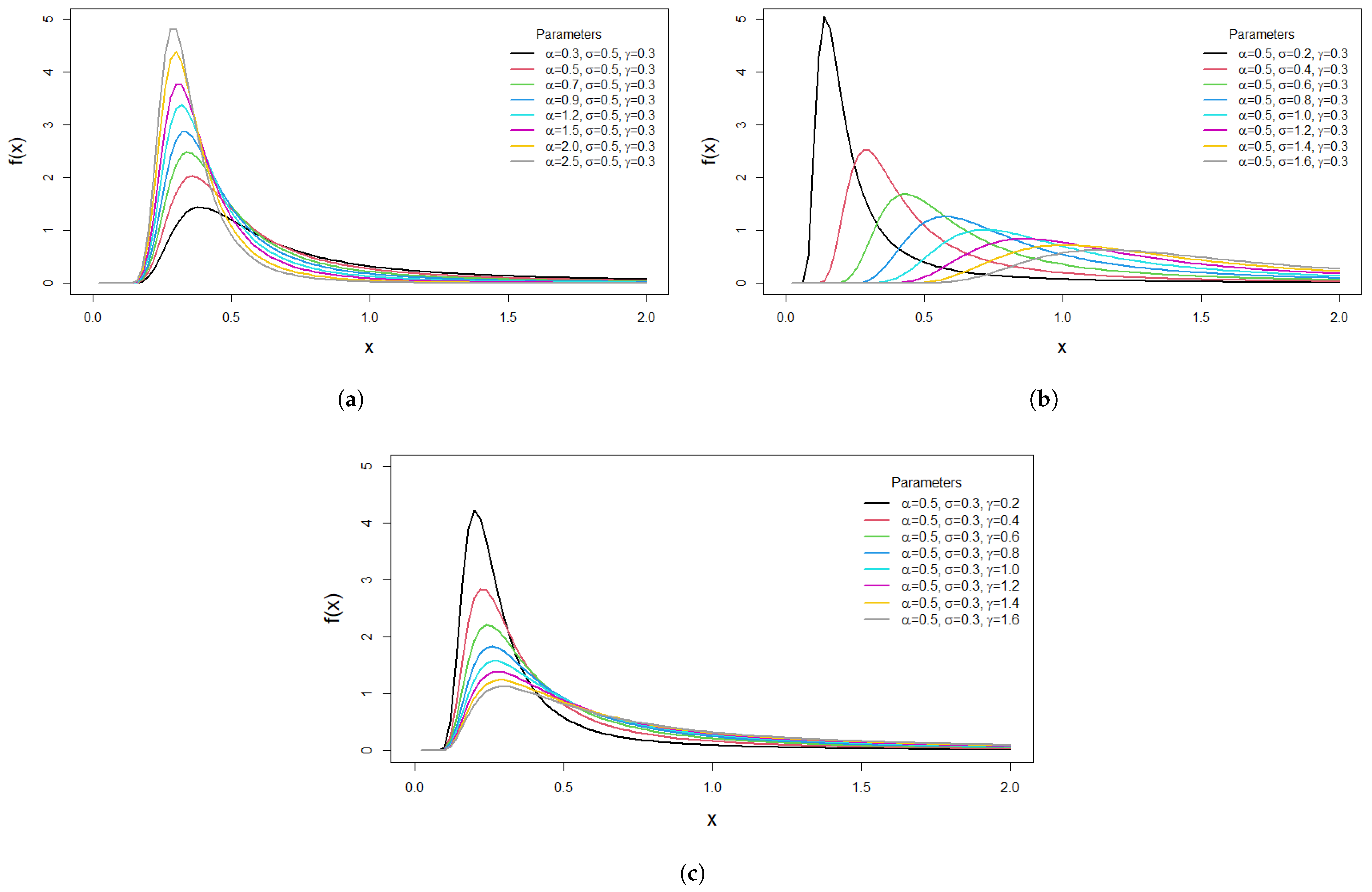
The plots in Figure 1a–c illustrate the PDF plots when changing one of the parameters and fixing the others. Figure 1a,c show different potential PDF shapes for the M-O-EIR distribution for various values of the shape parameters $\alpha$ and $\gamma$. It is obvious that the distribution is unimodal and right skewed, which is suitable in modeling asymmetric data. In Figure 1b, when the scale parameter $\sigma$ increases while the shape parameters $\alpha$ and $\gamma$ are fixed, the distribution expands to the right and its peak decreases. 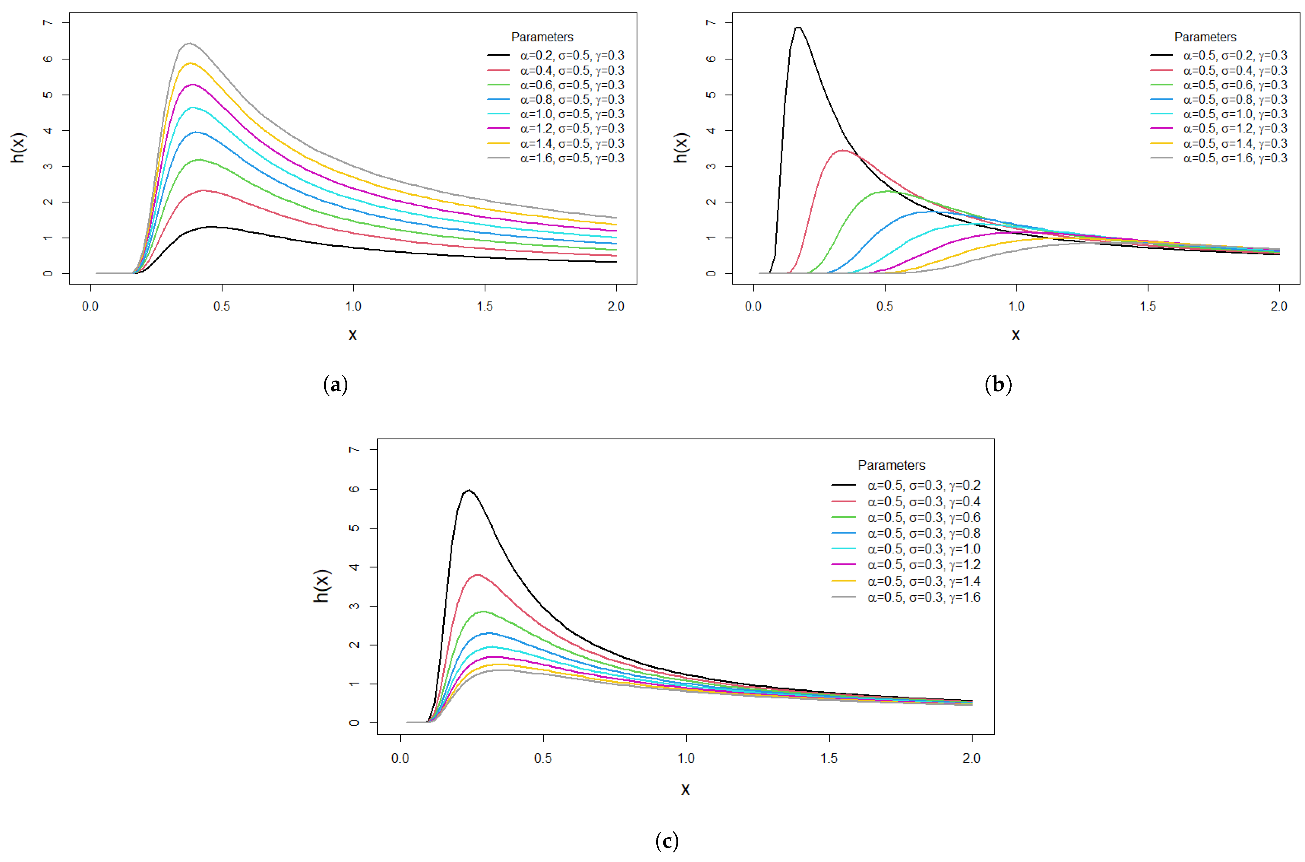The plots in Figure 2a–c demonstrate the behavior of the HRF for the M-O-EIR distribution. It is observed that the hazard rate function increases and then decreases with time, which is highly beneficial in survival analysis.

4. Statistical Properties

4.1. Moments

The rth moment can be applied to obtain most of the measures of central tendency and dispersion, including the mean, variance, skewness, and kurtosis. The rth moment of the M-O-EIR distribution is obtained as

$$E\left(X^r\right)={\int }_0^{\infty }{x}^{r}f\left(x\right)dx=2\alpha \gamma {\sigma }^2{\int }_0^{\infty }{\displaystyle \frac{x^{r-3}{e}^{-{(\sigma /x)}^2}{(1-e^{-{(\sigma /x)}^2})}^{\alpha -1}}{{(1-\overline{\gamma }{(1-e^{-{(\sigma /x)}^2})}^{\alpha })}^2}}dx.$$

Using the following expansion,

$${(1-y)}^{-m}=\sum _{i=0}^{\infty }{\displaystyle \frac{\mathsf{\Gamma }(m+i)}{\mathsf{\Gamma }\left(m\right)i!}}{y}^i,m>0,\left|y\right|<1,$$

(9)

we have

$$(1-\overline{\gamma }{(1-e^{-{(\sigma /x)}^2})}^{\alpha }{)}^{-2}=\sum _{i=0}^{\infty }(i+1){\overline{\gamma }}^i{(1-e^{-{(\sigma /x)}^2})}^{i\alpha }.$$

Therefore,

$$E\left(X^r\right)=\sum _{i=0}^{\infty }2\alpha (i+1)\gamma {\overline{\gamma }}^i{\sigma }^2{\int }_0^{\infty }{x}^{r-3}{e}^{-{(\sigma /x)}^2}{(1-e^{-{(\sigma /x)}^2})}^{\alpha (i+1)-1}dx.$$

(10)

Applying the following expansion to Equation (10),

$${(1-z)}^n=\sum _{j=0}^{\infty }\left({\displaystyle \genfrac{}{}{0pt}{}{n}{j}}\right){(-1)}^j{z}^j,n>0,\left|z\right|<1,$$

(11)

we obtain

$$E\left(X^r\right)=\sum _{i=0}^{\infty }\sum _{j=0}^{\infty }2\alpha (i+1)\gamma {\overline{\gamma }}^i{\sigma }^2{(-1)}^j\left({\displaystyle \genfrac{}{}{0pt}{}{\alpha (i+1)-1}{j}}\right){\int }_0^{\infty }{x}^{r-3}{e}^{-(j+1){(\sigma /x)}^2}dx.$$

(12)

Using integration by substitution, the rth moment of the M-O-EIR distribution is

$$E\left(X^r\right)=C{\displaystyle \frac{{\sigma }^{r-2}\mathsf{\Gamma }(\frac{-r}{2}+1)}{2{(j+1)}^{\frac{-r}{2}+1}}},r<2,$$

(13)

where $C={\sum }_{i=0}^{\infty }{\sum }_{j=0}^{\infty }2\alpha (i+1)\gamma {\overline{\gamma }}^i{\sigma }^2{(-1)}^j\left({\displaystyle \genfrac{}{}{0pt}{}{\alpha (i+1)-1}{j}}\right).$

4.2. Moment Generating Function

The moment generating function (MGF) of the random variable X, is defined as follows:

$$\begin{array}{cc}\hfill M_X\left(t\right)=E\left(e^{tx}\right)=& {\int }_0^{\infty }{e}^{tx}f\left(x\right)dx\hfill \\ \hfill =& {\int }_0^{\infty }\sum _{r=0}^{\infty }{\displaystyle \frac{{\left(tx\right)}^r}{r!}}f\left(x\right)dx\hfill \\ \hfill =& \sum _{r=0}^{\infty }{\displaystyle \frac{t^r}{r!}}{\int }_0^{\infty }{x}^{r}f\left(x\right)dx.\hfill \end{array}$$

(14)

Substituting Equation (13) in Equation (14), the MGF is

$$M_X\left(t\right)=C\sum _{r=0}^{\infty }{\displaystyle \frac{t^r}{r!}}{\displaystyle \frac{{\sigma }^{r-2}\mathsf{\Gamma }(\frac{-r}{2}+1)}{2{(j+1)}^{\frac{-r}{2}+1}}},$$

(15)

where $C={\sum }_{i=0}^{\infty }{\sum }_{j=0}^{\infty }2\alpha (i+1)\gamma {\overline{\gamma }}^i{\sigma }^2{(-1)}^j\left({\displaystyle \genfrac{}{}{0pt}{}{\alpha (i+1)}{j}}\right).$

4.3. Order Statistics

Let $x_{1:n},x_{2:n},\dots ,x_{n:n}$ be the order statistics from the M-O-EIR distribution. The kth order statistic can be obtained using the following definition:

$$f_{k:n}\left(x\right)={\displaystyle \frac{n!}{(k-1)!(n-k)!}}\left[f\left(x\right)\right]{\left[F\left(x\right)\right]}^{k-1}{[1-F\left(x\right)]}^{n-k}.$$

(16)

Applying the expansion in Equation (11) into Equation (16), we have

$$f_{k:n}\left(x\right)=\sum _{m=0}^{\infty }\left({\displaystyle \genfrac{}{}{0pt}{}{n-k}{m}}\right){(-1)}^m{\displaystyle \frac{n!}{(k-1)!(n-k)!}}f\left(x\right){\left[F\left(x\right)\right]}^{k+m-1}.$$

(17)

Substituting Equations (6) and (7) into Equation (17), we obtain

$$f_{k:n}\left(x\right)=c^{*}{\displaystyle \frac{e^{-{(\sigma /x)}^2}{(1-e^{-{(\sigma /x)}^2})}^{\alpha -1}{[1-{(1-e^{-{(\sigma /x)}^2})}^{\alpha }]}^{k+m-1}}{x^3{[1-\overline{\gamma }{(1-e^{-{(\sigma /x)}^2})}^{\alpha }]}^{k+m+1}}},$$

(18)

where $c^{*}=2\gamma \alpha {\sigma }^2{\sum }_{m=0}^{\infty }\left({\displaystyle \genfrac{}{}{0pt}{}{n-k}{m}}\right){(-1)}^m{\displaystyle \frac{n!}{(k-1)!(n-k)!}}$.

4.4. Rényi Entropy

The uncertainty of a random variable X can be measured by its entropy. The Rényi entropy of order $\theta$ of the random variable X is given by

$$R_{\theta }\left(x\right)={(1-\theta )}^{-1}log\left[{\int }_0^{\infty }{\left(f\left(x\right)\right)}^{\theta }dx\right],\theta >0,\theta \ne 1.$$

(19)

Substituting Equation (7) in Equation (19), yields

$$R_{\theta }\left(x\right)={(1-\theta )}^{-1}log\left[{\int }_0^{\infty }{\left(2\alpha \gamma {\sigma }^2\right)}^{\theta }{e}^{-\theta {(\sigma /x)}^2}{x}^{-3\theta }{(1-e^{-{(\sigma /x)}^2})}^{\theta (\alpha -1)}{[1-\overline{\gamma }{(1-e^{-{(\sigma /x)}^2})}^{\alpha }]}^{-2\theta }dx\right].$$

(20)

Therefore, by applying Equation (9) in Equation (20), we have

$$R_{\theta }\left(x\right)={(1-\theta )}^{-1}log\left[D_1{\int }_0^{\infty }{e}^{-\theta {(\sigma /x)}^2}{x}^{-3\theta }{(1-e^{-{(\sigma /x)}^2})}^{\theta (\alpha -1)+l\alpha }dx\right],$$

(21)

where $D_1={\sum }_{l=0}^{\infty }{\displaystyle \frac{\mathsf{\Gamma }(2\theta +l)}{\mathsf{\Gamma }\left(2\theta \right)l!}}{\left(2\alpha \gamma {\sigma }^2\right)}^{\theta }{\overline{\gamma }}^l$.

Additionally, by using the expansion in Equation (11), Equation (21) can be written as

$$R_{\theta }\left(x\right)={(1-\theta )}^{-1}log\left[D_2{\int }_0^{\infty }{x}^{-3\theta }{e}^{-(\theta +v){(\sigma /x)}^2}dx\right],$$

(22)

where $D_2=D_1{\sum }_{v=0}^{\infty }\left({\displaystyle \genfrac{}{}{0pt}{}{\theta (\alpha -1)+l\alpha }{v}}\right){(-1)}^v$. To solve Equation (22), let $u=(\theta +v){(\sigma /x)}^2$, then $x={\left({\displaystyle \frac{u}{{\sigma }^2(\theta +v)}}\right)}^{-1/2}$ and $dx={\displaystyle \frac{-1}{2}}{\left({\displaystyle \frac{u}{{\sigma }^2(\theta +v)}}\right)}^{-3/2}·{\displaystyle \frac{1}{{\sigma }^2(\theta +v)}}du$; hence, the Rényi entropy can be solved using the gamma function as follows:

$$\begin{array}{cc}\hfill R_{\theta }\left(x\right)& ={(1-\theta )}^{-1}log\left[D_3{\int }_0^{\infty }{u}^{{\displaystyle \frac{3}{2}}(\theta -1)}{e}^{-u}du\right]\hfill \\ \hfill & ={(1-\theta )}^{-1}log\left[D_3\mathsf{\Gamma }({\displaystyle \frac{3}{2}}(\theta -1)+1)\right],\hfill \end{array}$$

(23)

where $D_3=D_2·{\displaystyle \frac{1}{2{\left({\sigma }^2(\theta +v)\right)}^{\frac{3}{2}\theta -1/2}}}$.

Table 1. Rényi entropy for $\alpha =1.5,2$, $\sigma =1.5$, $\gamma =0.3$, and $\theta =0.5,1.5,2$.

$\mathit{\alpha }$	$\mathit{\sigma }$	$\mathit{\gamma }$	$\mathit{\theta }$	Rényi Entropy
1.5	1.5	0.3	0.5	1.9202
1.5	1.5	0.3	1.5	0.8240
1.5	1.5	0.3	2	0.7646
2	1.5	0.3	0.5	1.6131
2	1.5	0.3	1.5	0.9003
2	1.5	0.3	2	0.9029

,

Table 2. Rényi entropy for $\alpha =1.5$, $\sigma =2.5,3.5$, $\gamma =0.3$, and $\theta =0.5,1.5,2$.

$\mathit{\alpha }$	$\mathit{\sigma }$	$\mathit{\gamma }$	$\mathit{\theta }$	Rényi Entropy
1.5	2.5	0.3	0.5	2.4789
1.5	2.5	0.3	1.5	0.6383
1.5	2.5	0.3	2	0.4588
1.5	3.5	0.3	0.5	2.9330
1.5	3.5	0.3	1.5	0.5394
1.5	3.5	0.3	2	0.3277

and

Table 3. Rényi entropy for $\alpha =0.6$, $\sigma =0.3$, $\gamma =1.2,2.6$, and $\theta =0.5,1.5,2$.

$\mathit{\alpha }$	$\mathit{\sigma }$	$\mathit{\gamma }$	$\mathit{\theta }$	Rényi Entropy
0.6	0.3	1.2	0.5	6.5772
0.6	0.3	1.2	1.5	0.8180
0.6	0.3	1.2	2	0.8163
0.6	0.3	2.6	0.5	9.0528
0.6	0.3	2.6	1.5	0.6101
0.6	0.3	2.6	2	0.4584

illustrate the results of the Rényi entropy for the M-O-EIR distribution at different parameters of $\alpha$, $\sigma$, and $\gamma$ when $\theta$ = 0.5, 1.5, and 2. It is observed that the Rényi entropy decreases with increasing $\theta$ from 0.5 to 2. This indicates that the uncertainty associated with the distribution also decreases, implying that fewer bits of information are required to represent the random variable. More specifically, in Table 1, when $\alpha$ changes from 1.5 to 2 while the other parameters are fixed ($\sigma =1.5$, $\gamma =0.3$), the Rényi entropy decreases when $\theta =0.5$ and increases when $\theta =1.5$ and 2. Table 2 demonstrates the entropy when $\sigma$ changes from 2.5 to 3.5, while the other parameters are fixed ($\alpha$ = 1.5, $\gamma$ = 0.3) at $\theta$ = 0.5, 1.5, 2. It is clear that the entropy increases when $\theta$ = 0.5, and decreases when $\theta$ = 1.5 and 2. Finally, when $\gamma$ increases from 1.2 to 2.6 while the other parameters are fixed, ($\alpha$ = 0.6, $\sigma =0.3$), the entropy increases at $\theta$ = 0.5 and decreases at $\theta$ = 1.5 and 2, as demonstrated in Table 3. As a result, an increase in Rényi entropy as the distribution parameters increase indicates that the probability density becomes more dispersed over the support of the distribution. Conversely, a decrease in Rényi entropy with increasing parameters indicates that the probability density is becoming more concentrated in specific regions of the distribution’s support. This leads to reduced uncertainty.

4.5. Quantile

Let X be a random variable following the M-O-EIR distribution. The quantile function of the random variable X can be derived using Equation (3) as follows:

$$P={\displaystyle \frac{G\left(x\right)}{1-\overline{\gamma }\overline{G}\left(x\right)}},$$

(24)

where P belongs to the uniform distribution in [0, 1]. Then, by substituting Equation (1) in Equation (24) and using certain algebraic operations, the quantile function is given by

$$Q\left(P\right)=G^{-1}\left(P\right)={\displaystyle \frac{\sigma }{{[-\log [1-{\left(\frac{1-P}{1-\overline{\gamma }P}\right)}^{1/\alpha }]]}^{1/2}}}·$$

(25)

In simulation, random samples are generated using the quantile function in Equation (25) for different sample sizes to estimate the parameters of the EIR-MO distribution.

The first, second (median), and third quartiles can be obtained when $P=0.25,0.5,$ and $0.75$, respectively.

5. Maximum Likelihood Estimation

Let $x=(x_1,x_2,\dots ,x_n)$ be an independent random sample of size n from the M-O-EIR distribution. The log likelihood function of parameters $\alpha ,\sigma ,$ and $\gamma$ is given by

$$\begin{array}{cc}\hfill l\left(\underline{x}\right|\alpha ,\sigma ,\gamma )& =\log \prod _{i=1}^{n}f(x_i;\alpha ,\sigma ,\gamma )=n\left(\log 2\gamma \alpha {\sigma }^2\right)\hfill \\ \hfill & -\sum _{i=1}^n\left[{(\sigma /x_i)}^2-\log {(1-e^{-{(\sigma /x_i)}^2})}^{\alpha -1}+3\log \left(x_i\right)+\log {[1-\overline{\gamma }{(1-e^{-{(\sigma /x_i)}^2})}^{\alpha }]}^2\right]·\hfill \end{array}$$

(26)

The first partial derivatives of the log likelihood function $l\left(\underline{x}\right|\alpha ,\sigma ,\gamma )$ with respect to the parameters $\alpha ,\sigma$, and $\gamma$ are obtained to find the estimates $\widehat{\alpha },\widehat{\sigma }$, and $\widehat{\gamma }$ that maximize the likelihood function, as follows:

$${\displaystyle \frac{\partial l\left(\underline{x}\right|\alpha ,\sigma ,\gamma )}{\partial \alpha }}={\displaystyle \frac{n}{\alpha }}+\sum _{i=1}^n\left[log(1-e^{-{(\sigma /x_i)}^2})+{\displaystyle \frac{2\overline{\gamma }{(1-e^{-{(\sigma /x_i)}^2})}^{\alpha }log(1-e^{-{(\sigma /x_i)}^2})}{1-\overline{\gamma }{(1-e^{-{(\sigma /x_i)}^2})}^{\alpha }}}\right],$$

(27)

$${\displaystyle \frac{\partial l\left(\underline{x}\right|\alpha ,\sigma ,\gamma )}{\partial \sigma }}={\displaystyle \frac{2n}{\sigma }}-\sum _{i=1}^n\left[{\displaystyle \frac{2\sigma }{x_i^2}}-{\displaystyle \frac{2(\alpha -1)\sigma e^{-{(\sigma /x_i)}^2}}{(1-e^{-{(\sigma /x_i)}^2})x_i^2}}-{\displaystyle \frac{4\overline{\gamma }\alpha e^{-{(\sigma /x_i)}^2}{(1-e^{-{(\sigma /x_i)}^2})}^{\alpha -1}\sigma }{x_i^2[1-\overline{\gamma }{(1-e^{-{(\sigma /x_i)}^2})}^{\alpha }]}}\right],$$

(28)

and

$${\displaystyle \frac{\partial l\left(\underline{x}\right|\alpha ,\sigma ,\gamma )}{\partial \gamma }}={\displaystyle \frac{n}{\gamma }}-\sum _{i=1}^n\left[{\displaystyle \frac{2{(1-e^{-{(\sigma /x_i)}^2})}^{\alpha }}{1-\overline{\gamma }{(1-e^{-{(\sigma /x_i)}^2})}^{\alpha }}}\right].$$

(29)

By equating Equations (27)–(29) to zero and solving them numerically using R language 2022.07.2 Build 576, we obtain the maximum likelihood estimates of the parameters $\alpha$, $\sigma$ and $\gamma$.

6. Bayesian Estimation

Bayesian estimation is a statistical method that uses prior distribution for estimating the value of an unknown parameter. Many authors have contributed in studying Bayesian estimation: see Aboraya et al. [22], Eliwa et al. [23], Elbatal et al. [24], and Alotaibi et al. [25]. Assume that the independent prior distributions of the parameters $\alpha$, $\sigma$, and $\gamma$ are gamma distributions, that is, $\alpha \sim G(a_1,w_1)$, $\sigma \sim G(a_2,w_2)$, and $\gamma \sim G(a_3,w_3)$. Therefore, the joint prior density can be expressed as

$$\pi (\alpha ,\sigma ,\gamma )\propto {\alpha }^{a_1-1}{\sigma }^{a_2-1}{\gamma }^{a_3-1}{e}^{-(w_1\alpha +w_2\sigma +w_3\gamma )},$$

(30)

where $a_1,a_2,a_3,w_1,w_2,$ and $w_3$ are the hyper-parameters of the prior distribution, all of which are positive constants.

The joint posterior density function of $\alpha$, $\sigma$, and $\gamma$ is obtained by multiplying the likelihood function and the joint prior density of the parameters, as follows:

$$\begin{array}{cc}\hfill \pi (\alpha ,\sigma ,\gamma |\underline{x})& \propto L\left(\underline{x}\right|\alpha ,\sigma ,\gamma )\pi (\alpha ,\sigma ,\gamma ),\hfill \\ \hfill & \propto {\alpha }^{a_1-1}{\sigma }^{a_2-1}{\gamma }^{a_3-1}{e}^{-(w_1\alpha +w_2\sigma +w_3\gamma )}\prod _{i=1}^n{\displaystyle \frac{2\alpha \gamma {\sigma }^2{e}^{-{(\sigma /x)}^2}{(1-e^{-{(\sigma /x)}^2})}^{\alpha -1}}{x^3{[1-\overline{\gamma }{(1-e^{-{(\sigma /x)}^2})}^{\alpha }]}^2}}·\hfill \end{array}$$

(31)

Therefore, the conditional posterior density functions of the parameters $\alpha$, $\sigma$, and $\gamma$ are obtained from Equation (31), as follows:

$$\pi \left(\alpha \right|\sigma ,\gamma ,\underline{x})\propto {\alpha }^{a_1+n-1}{e}^{-w_1\alpha }\prod _{i=1}^n{\displaystyle \frac{{(1-e^{-{(\sigma /x)}^2})}^{\alpha -1}}{{[1-\overline{\gamma }{(1-e^{-{(\sigma /x)}^2})}^{\alpha }]}^2}},$$

(32)

$$\pi \left(\sigma \right|\alpha ,\gamma ,\underline{x})\propto {\sigma }^{a_2+2n-1}{e}^{-w_2\sigma -n{(\sigma /x)}^2}\prod _{i=1}^n{\displaystyle \frac{{(1-e^{-{(\sigma /x)}^2})}^{\alpha -1}}{{[1-\overline{\gamma }{(1-e^{-{(\sigma /x)}^2})}^{\alpha }]}^2}},$$

(33)

$$\pi \left(\gamma \right|\alpha ,\sigma ,\underline{x})\propto {\gamma }^{a_3+n-1}{e}^{-w_3\gamma }\prod _{i=1}^n{[1-\overline{\gamma }{(1-e^{-{(\sigma /x)}^2})}^{\alpha }]}^{-2}.$$

(34)

In most cases, Bayesian estimation is employed under the squared-error loss function (SELF), which is the mean of the marginal of the parameter. The Bayesian estimators of the parameters $\alpha$, $\sigma$, and $\gamma$ regarding SELF are given as follows:

$$\begin{array}{cc}\hfill \tilde{\alpha }& =E\left(\alpha \right|\sigma ,\gamma ,\underline{x}),\hfill \\ \hfill \tilde{\sigma }& =E\left(\sigma \right|\alpha ,\gamma ,\underline{x}),\hfill \\ \hfill \tilde{\gamma }& =E\left(\gamma \right|\alpha ,\sigma ,\underline{x})·\hfill \end{array}$$

(35)

However, it is not possible to apply Equation (35) directly. Hence, numerical approximations will be applied using the Gibbs sampler algorithm 1 to obtain random samples of conditional posterior density functions in Equations (32)–(34). This algorithm describes the implementation of Gibbs sampling to estimate parameters $\alpha$, $\sigma$, and $\gamma$ of a statistical model as follows:

Algorithm 1 Gibbs Sampler Algorithm

1: Prior Distribution Initialization:   2: Define hyper-parameters for gamma prior distributions:   3: $a_1,w_1$ for $\alpha$, $a_2,w_2$ for $\sigma$, and $a_3,w_3$ for $\gamma$.   4: Density Function $dM-O-EIR(x,\alpha ,\sigma ,\gamma )$:   5:      ${\displaystyle \frac{\gamma (2\alpha {\sigma }^2/x^3)exp\left(-{(\sigma /x)}^2\right){(1-exp\left(-{(\sigma /x)}^2\right))}^{\alpha -1}}{{(1-\overline{\gamma }{(1-exp\left(-{(\sigma /x)}^2\right))}^{\alpha })}^2}}$   6: Quantile Function $qMOC(p,\gamma ,\sigma ,\alpha )$:   7:      $\sigma /\sqrt{-log(1-{(1-p)}^{1/\alpha })}$   8: Distribution Function $pMOC(q,\gamma ,\sigma ,\alpha )$:   9:      Numerically find q for given $p,\gamma ,\sigma ,\alpha$. 10: Random Generation $rMOC(n,\gamma ,\sigma ,\alpha )$: 11:      Generate n random variables. 12: Gibbs Sampling Steps: 13: Define the conditional posterior distributions in Equations (32)–(34) 14: Initialize the parameters ${\alpha }_0$, ${\sigma }_0$, ${\gamma }_0$ using prior information. 15: for $iter=1$ to $N_{iter}$ do 16:     Draw a sample ${\alpha }_i$ from the conditional posterior $\pi \left(\alpha \right|{\sigma }_{i-1},{\gamma }_{i-1},\underline{x})$ 17:     Update $\alpha$ given current $\sigma$, $\gamma$ and hyper-parameters $a_1,w_1$. 18:     Draw a sample ${\sigma }_i$ from the conditional posterior $\pi \left(\sigma \right|{\alpha }_i,{\gamma }_{i-1},\underline{x})$ 19:     Update $\sigma$ given current $\alpha$, $\gamma$ and hyper-parameters $a_2,w_2$. 20:     Draw a sample ${\gamma }_i$ from the conditional posterior $\pi \left(\gamma \right|{\alpha }_i,{\sigma }_i,\underline{x})$ 21:     Update $\gamma$ given current $\alpha$, $\sigma$ and hyper-parameters $a_3,w_3$. 22: end for 23: Output: Estimated parameters $\alpha$, $\sigma$, $\gamma$.

For more details, see Mohamed et al. [17], Aboraya et al. [22], and Elbatal et al. [24].

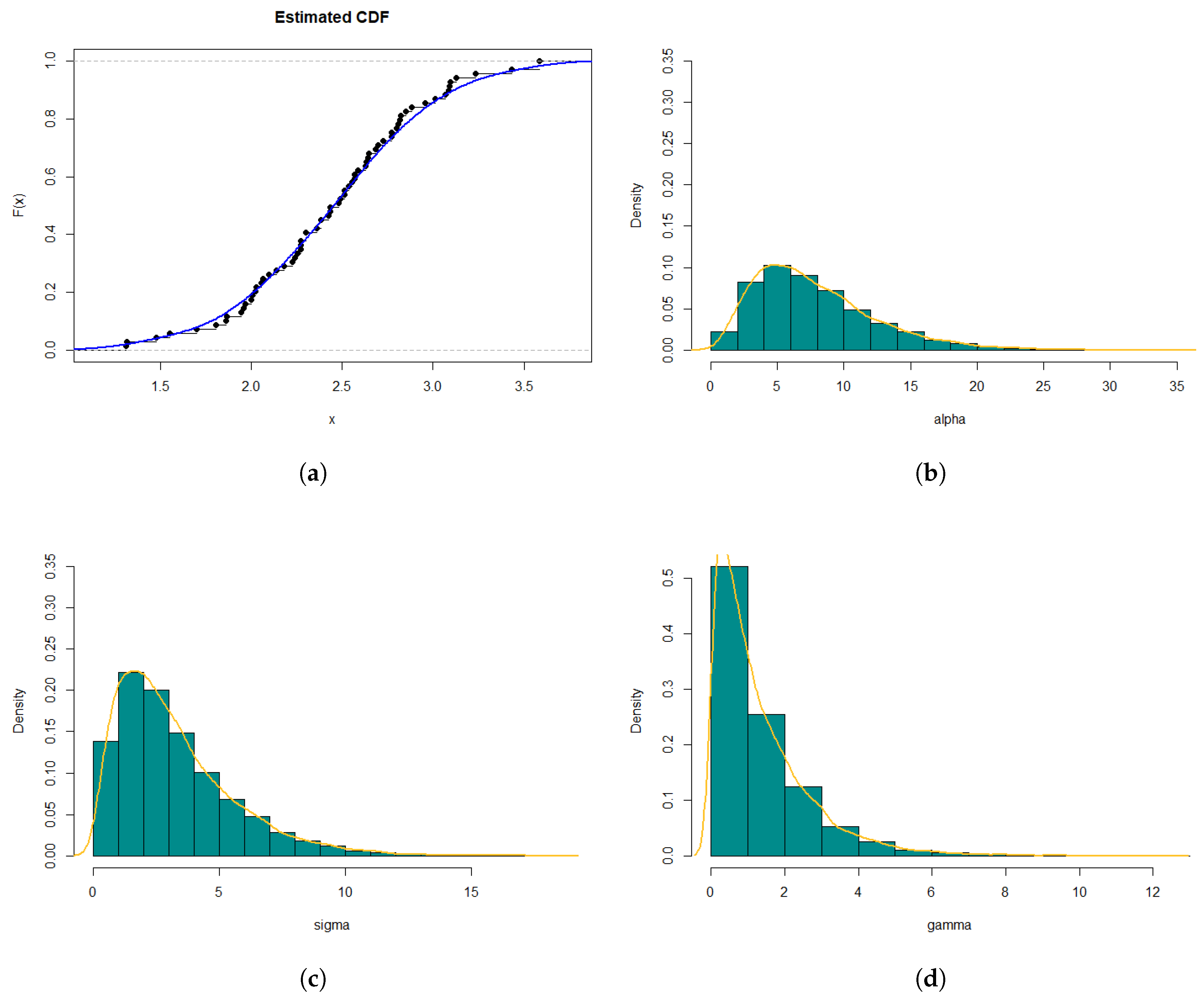
7. Simulation Studies

In this section, simulation studies were conducted using the R programming language to evaluate the theoretical results of the estimation process. Tables Table 4, Table 6, and Table 8 present the maximum likelihood (ML) estimation results for parameters $\alpha$, $\sigma$, and $\gamma$ for different sample sizes. The initial values of the parameters were chosen randomly in three cases:

• Case 1: (Table 1) $\alpha =0.6$, $\sigma =0.9$, and $\gamma =1.5$.
• Case 2: (Table 3) $\alpha =2.3$, $\sigma =1.5$, and $\gamma =1.8$.
• Case 3: (Table 5) $\alpha =0.7$, $\sigma =0.8$, and $\gamma =0.9$.

The tables provide the ML estimates, bias, mean squared error (MSE), 95% confidence interval (lower limit, upper limit), and the length of the confidence interval for each parameter.

For example, in Table 4 and for $n=150$, the ML estimates are $\alpha =0.5771750$, $\sigma =0.9234943$, and $\gamma =1.5719552$. The bias represents the difference between the ML estimate and the true value of the parameter, so for $\alpha$, the bias is approximately $-0.02282498$. The MSE provides a measure of the accuracy of the estimation, with lower values indicating better estimation performance. The 95% confidence interval gives a range of plausible values for the estimate of parameters, where the lower limit and upper limit represent the lower and upper bounds of the interval, respectively. The length of the confidence interval measures the width of the interval.

Table 5, Table 7, and Table 9 present the Gibbs estimation results for the initial guess of the parameters in Cases 1, 2, and 3, along with the sample sizes ($n=150,200,300,400$). Additionally, they provide the Gibbs estimates, bias, MSE, 95% confidence interval (lower limit, upper limit), and the length of the confidence interval.

For example, in Table 5 and for $n=150$, the Gibbs estimates are $\alpha =0.6145842$, $\sigma =0.8986206$, and $\gamma =1.5177550$. The bias is the difference between the Gibbs estimate and the true value of the parameter. The MSE measures the accuracy of the Gibbs estimation. The 95% confidence interval provides a range of plausible values for the estimate, and the length of the interval indicates its width.

The tables given allow us to assess how the ML estimation performs in relation to the Gibbs estimation method for different sample sizes. It is observed that the Gibbs method performs better since it provides smaller biases, smaller MSEs, and narrower confidence intervals.

Table 4. ML estimates of the parameters $\alpha =0.6$, $\sigma =0.9$, and $\gamma =1.5$ for sample sizes $n=150,200,300,400$.

n	Parameter	95% Confidence Interval					Length
		ML Estimate	Bias	MSE	Lower Limit	Upper Limit
	$\alpha$	0.5771750	−0.02282498	0.004838136	0.4690902	0.6852599	0.2161697
150	$\sigma$	0.9234943	0.02349434	0.012781062	0.7415818	1.1054069	0.3638252
	$\gamma$	1.5719552	0.07195516	0.393476985	0.5468952	2.5970152	2.0501200
	$\alpha$	0.6213724	0.02137245	0.005566749	0.5037812	0.7389637	0.2351825
200	$\sigma$	0.8760288	−0.02397124	0.007869966	0.7355247	1.0165328	0.2810081
	$\gamma$	1.8002179	0.30021791	0.432649746	0.8374797	2.7629561	1.9254764
	$\alpha$	0.5802084	−0.019791619	0.005113568	0.4671709	0.6932459	0.2260749
300	$\sigma$	0.9064734	0.006473443	0.005329572	0.7868551	1.0260918	0.2392368
	$\gamma$	1.4749322	−0.025067831	0.264474681	0.6299620	2.3199024	1.6899404
	$\alpha$	0.6304493	0.030449308	0.003509457	0.5468565	0.7140421	0.1671856
400	$\sigma$	0.9073363	0.007336349	0.001354344	0.8480131	0.9666596	0.1186464
	$\gamma$	1.5793075	0.079307471	0.106944222	1.0574131	2.1012018	1.0437887

Table 4. ML estimates of the parameters $\alpha =0.6$, $\sigma =0.9$, and $\gamma =1.5$ for sample sizes $n=150,200,300,400$.

n	Parameter	95% Confidence Interval					Length
		ML Estimate	Bias	MSE	Lower Limit	Upper Limit
	$\alpha$	0.5771750	−0.02282498	0.004838136	0.4690902	0.6852599	0.2161697
150	$\sigma$	0.9234943	0.02349434	0.012781062	0.7415818	1.1054069	0.3638252
	$\gamma$	1.5719552	0.07195516	0.393476985	0.5468952	2.5970152	2.0501200
	$\alpha$	0.6213724	0.02137245	0.005566749	0.5037812	0.7389637	0.2351825
200	$\sigma$	0.8760288	−0.02397124	0.007869966	0.7355247	1.0165328	0.2810081
	$\gamma$	1.8002179	0.30021791	0.432649746	0.8374797	2.7629561	1.9254764
	$\alpha$	0.5802084	−0.019791619	0.005113568	0.4671709	0.6932459	0.2260749
300	$\sigma$	0.9064734	0.006473443	0.005329572	0.7868551	1.0260918	0.2392368
	$\gamma$	1.4749322	−0.025067831	0.264474681	0.6299620	2.3199024	1.6899404
	$\alpha$	0.6304493	0.030449308	0.003509457	0.5468565	0.7140421	0.1671856
400	$\sigma$	0.9073363	0.007336349	0.001354344	0.8480131	0.9666596	0.1186464
	$\gamma$	1.5793075	0.079307471	0.106944222	1.0574131	2.1012018	1.0437887

Table 5. Gibbs estimates of the parameters $\alpha =0.6$, $\sigma =0.9$, and $\gamma =1.5$ for sample sizes $n=150,200,300,400$.

n	Parameter	95% Confidence Interval					Length
		Gibbs Estimate	Bias	MSE	Lower Limit	Upper Limit
150	$\alpha$	0.6145842	0.009843254	0.0009402291	0.5668129	0.6623555	0.09554261
	$\sigma$	0.8986206	0.023575332	0.0017916399	0.8407913	0.9564499	0.11565853
	$\gamma$	1.5177550	0.115959169	0.0167852140	1.4227046	1.6128053	0.19010066
200	$\alpha$	0.6142425	0.04944098	0.003039235	0.5741225	0.6543624	0.08023986
	$\sigma$	0.9436900	0.01171312	0.001074259	0.8933342	0.9940459	0.10071170
	$\gamma$	1.5629566	−0.01958582	0.006698013	1.4322395	1.6936736	0.26143411
300	$\alpha$	0.6102177	0.01796004	0.0007921347	0.5745712	0.6458642	0.07129299
	$\sigma$	0.9287885	−0.04775314	0.0035509068	0.8701530	0.9874240	0.11727103
	$\gamma$	1.5054043	0.02681624	0.0038531711	1.4133128	1.5974958	0.18418302
400	$\alpha$	0.6224760	0.0035316688	0.0005690846	0.5836662	0.6612859	0.07761973
	$\sigma$	0.9026814	0.0003655791	0.0030841192	0.8113286	0.9940343	0.18270569
	$\gamma$	1.5033342	−0.0227326067	0.0051544409	1.3913090	1.6153594	0.22405044

Table 5. Gibbs estimates of the parameters $\alpha =0.6$, $\sigma =0.9$, and $\gamma =1.5$ for sample sizes $n=150,200,300,400$.

n	Parameter	95% Confidence Interval					Length
		Gibbs Estimate	Bias	MSE	Lower Limit	Upper Limit
150	$\alpha$	0.6145842	0.009843254	0.0009402291	0.5668129	0.6623555	0.09554261
	$\sigma$	0.8986206	0.023575332	0.0017916399	0.8407913	0.9564499	0.11565853
	$\gamma$	1.5177550	0.115959169	0.0167852140	1.4227046	1.6128053	0.19010066
200	$\alpha$	0.6142425	0.04944098	0.003039235	0.5741225	0.6543624	0.08023986
	$\sigma$	0.9436900	0.01171312	0.001074259	0.8933342	0.9940459	0.10071170
	$\gamma$	1.5629566	−0.01958582	0.006698013	1.4322395	1.6936736	0.26143411
300	$\alpha$	0.6102177	0.01796004	0.0007921347	0.5745712	0.6458642	0.07129299
	$\sigma$	0.9287885	−0.04775314	0.0035509068	0.8701530	0.9874240	0.11727103
	$\gamma$	1.5054043	0.02681624	0.0038531711	1.4133128	1.5974958	0.18418302
400	$\alpha$	0.6224760	0.0035316688	0.0005690846	0.5836662	0.6612859	0.07761973
	$\sigma$	0.9026814	0.0003655791	0.0030841192	0.8113286	0.9940343	0.18270569
	$\gamma$	1.5033342	−0.0227326067	0.0051544409	1.3913090	1.6153594	0.22405044

Table 6. ML estimates of the parameters $\alpha =2.3$, $\sigma =1.5$, and $\gamma =1.8$ for sample sizes $n=100,200,300,400$.

n	Parameter	95% Confidence Interval					Length
		ML Estimate	Bias	MSE	Lower Limit	Upper Limit
100	$\alpha$	2.153459	0.430914710	0.34059358	1.506018	2.800900	1.2948819
	$\sigma$	1.688962	−0.001248683	0.02621104	1.422648	1.955277	0.5326293
	$\gamma$	1.786701	0.051803699	0.01235204	1.624951	1.948451	0.3234995
200	$\alpha$	2.234282	−0.464169284	0.249594891	1.930327	2.538236	0.6079094
	$\sigma$	1.734226	−0.009221691	0.058223948	1.337584	2.130869	0.7932852
	$\gamma$	1.761486	0.018666838	0.005229557	1.646558	1.876413	0.2298556
300	$\alpha$	2.218313	−0.49967587	0.32090158	1.779294	2.657333	0.8780394
	$\sigma$	1.656387	0.09621738	0.02528184	1.448152	1.864621	0.4164684
	$\gamma$	1.874647	−0.03478232	0.03313397	1.580730	2.168565	0.5878353
400	$\alpha$	2.459155	0.01687739	0.49148448	1.306246	3.612063	2.3058174
	$\sigma$	1.706396	0.01827464	0.03103875	1.418146	1.994646	0.5764995
	$\gamma$	1.805303	0.01271099	0.03361914	1.504410	2.106197	0.6017874

Table 6. ML estimates of the parameters $\alpha =2.3$, $\sigma =1.5$, and $\gamma =1.8$ for sample sizes $n=100,200,300,400$.

n	Parameter	95% Confidence Interval					Length
		ML Estimate	Bias	MSE	Lower Limit	Upper Limit
100	$\alpha$	2.153459	0.430914710	0.34059358	1.506018	2.800900	1.2948819
	$\sigma$	1.688962	−0.001248683	0.02621104	1.422648	1.955277	0.5326293
	$\gamma$	1.786701	0.051803699	0.01235204	1.624951	1.948451	0.3234995
200	$\alpha$	2.234282	−0.464169284	0.249594891	1.930327	2.538236	0.6079094
	$\sigma$	1.734226	−0.009221691	0.058223948	1.337584	2.130869	0.7932852
	$\gamma$	1.761486	0.018666838	0.005229557	1.646558	1.876413	0.2298556
300	$\alpha$	2.218313	−0.49967587	0.32090158	1.779294	2.657333	0.8780394
	$\sigma$	1.656387	0.09621738	0.02528184	1.448152	1.864621	0.4164684
	$\gamma$	1.874647	−0.03478232	0.03313397	1.580730	2.168565	0.5878353
400	$\alpha$	2.459155	0.01687739	0.49148448	1.306246	3.612063	2.3058174
	$\sigma$	1.706396	0.01827464	0.03103875	1.418146	1.994646	0.5764995
	$\gamma$	1.805303	0.01271099	0.03361914	1.504410	2.106197	0.6017874

Table 7. Gibbs estimates of the parameters $\alpha =2.3$, $\sigma =1.5$, and $\gamma =1.8$ for sample sizes $n=100,200,300,400$.

n	Parameter	95% Confidence Interval					Length
		Gibbs Estimate	Bias	MSE	Lower Limit	Upper Limit
100	$\alpha$	2.448847	0.2197759	0.25828077	1.695051	3.202644	1.5075932
	$\sigma$	1.634007	−0.1146412	0.03801343	1.374582	1.893431	0.5188489
	$\gamma$	1.799770	−0.1784849	0.03917636	1.659033	1.940506	0.2814732
200	$\alpha$	2.273107	−0.180399658	0.11908250	1.789191	2.757024	0.9678331
	$\sigma$	1.676353	−0.006822676	0.02219400	1.431544	1.921162	0.4896185
	$\gamma$	1.823658	−0.084395585	0.02146485	1.626654	2.020661	0.3940073
300	$\alpha$	2.327360	0.406830338	0.226867665	1.919888	2.734831	0.8149426
	$\sigma$	1.636862	−0.008154544	0.009547621	1.476687	1.797038	0.3203508
	$\gamma$	1.865932	0.100229560	0.049332036	1.539882	2.191983	0.6521015
400	$\alpha$	2.301370	0.002194087	0.12992529	1.708438	2.894302	1.1858635
	$\sigma$	1.581303	0.100249401	0.02129398	1.406870	1.755735	0.3488647
	$\gamma$	1.803557	0.117629491	0.02659310	1.617764	1.989351	0.3715866

Table 7. Gibbs estimates of the parameters $\alpha =2.3$, $\sigma =1.5$, and $\gamma =1.8$ for sample sizes $n=100,200,300,400$.

n	Parameter	95% Confidence Interval					Length
		Gibbs Estimate	Bias	MSE	Lower Limit	Upper Limit
100	$\alpha$	2.448847	0.2197759	0.25828077	1.695051	3.202644	1.5075932
	$\sigma$	1.634007	−0.1146412	0.03801343	1.374582	1.893431	0.5188489
	$\gamma$	1.799770	−0.1784849	0.03917636	1.659033	1.940506	0.2814732
200	$\alpha$	2.273107	−0.180399658	0.11908250	1.789191	2.757024	0.9678331
	$\sigma$	1.676353	−0.006822676	0.02219400	1.431544	1.921162	0.4896185
	$\gamma$	1.823658	−0.084395585	0.02146485	1.626654	2.020661	0.3940073
300	$\alpha$	2.327360	0.406830338	0.226867665	1.919888	2.734831	0.8149426
	$\sigma$	1.636862	−0.008154544	0.009547621	1.476687	1.797038	0.3203508
	$\gamma$	1.865932	0.100229560	0.049332036	1.539882	2.191983	0.6521015
400	$\alpha$	2.301370	0.002194087	0.12992529	1.708438	2.894302	1.1858635
	$\sigma$	1.581303	0.100249401	0.02129398	1.406870	1.755735	0.3488647
	$\gamma$	1.803557	0.117629491	0.02659310	1.617764	1.989351	0.3715866

Table 8. ML estimates of the parameters $\alpha =0.7$, $\sigma =0.8$, and $\gamma =0.9$ for sample sizes $n=100,200,300,400$.

n	Parameter	95% Confidence Interval					Length
		ML Estimate	Bias	MSE	Lower Limit	Upper Limit
100	$\alpha$	0.8316659	$-1.752292\times {10}^{-2}$	0.0011159390	0.7848806	0.8784513	0.09357065
	$\sigma$	0.8163681	$-5.329821\times {10}^{-5}$	0.0005374803	0.7782312	0.8545051	0.07627391
	$\gamma$	0.9579443	$3.793317\times {10}^{-2}$	0.0018889469	0.9230478	0.9928409	0.06979311
200	$\alpha$	0.8271646	0.0002249037	0.0011891715	0.7704390	0.8838902	0.11345115
	$\sigma$	0.8434598	0.0384664282	0.0030380032	0.7785221	0.9083975	0.12987531
	$\gamma$	0.9548462	-0.0059776642	0.0003291505	0.9266683	0.9830242	0.05635589
300	$\alpha$	0.8685745	−0.086366396	0.0118576480	0.7594763	0.9776728	0.21819655
	$\sigma$	0.8265717	−0.048953817	0.0032391426	0.7788195	0.8743239	0.09550447
	$\gamma$	0.9640693	0.006154031	0.0009376036	0.9147266	1.0134119	0.09868528
400	$\alpha$	0.8709748	−0.16175433	0.030191820	0.7665807	0.9753689	0.20878817
	$\sigma$	0.8352936	0.01690962	0.001155469	0.7867861	0.8838011	0.09701504
	$\gamma$	0.9497568	−0.01820171	0.001278391	0.8991322	1.0003813	0.10124911

Table 8. ML estimates of the parameters $\alpha =0.7$, $\sigma =0.8$, and $\gamma =0.9$ for sample sizes $n=100,200,300,400$.

n	Parameter	95% Confidence Interval					Length
		ML Estimate	Bias	MSE	Lower Limit	Upper Limit
100	$\alpha$	0.8316659	$-1.752292\times {10}^{-2}$	0.0011159390	0.7848806	0.8784513	0.09357065
	$\sigma$	0.8163681	$-5.329821\times {10}^{-5}$	0.0005374803	0.7782312	0.8545051	0.07627391
	$\gamma$	0.9579443	$3.793317\times {10}^{-2}$	0.0018889469	0.9230478	0.9928409	0.06979311
200	$\alpha$	0.8271646	0.0002249037	0.0011891715	0.7704390	0.8838902	0.11345115
	$\sigma$	0.8434598	0.0384664282	0.0030380032	0.7785221	0.9083975	0.12987531
	$\gamma$	0.9548462	-0.0059776642	0.0003291505	0.9266683	0.9830242	0.05635589
300	$\alpha$	0.8685745	−0.086366396	0.0118576480	0.7594763	0.9776728	0.21819655
	$\sigma$	0.8265717	−0.048953817	0.0032391426	0.7788195	0.8743239	0.09550447
	$\gamma$	0.9640693	0.006154031	0.0009376036	0.9147266	1.0134119	0.09868528
400	$\alpha$	0.8709748	−0.16175433	0.030191820	0.7665807	0.9753689	0.20878817
	$\sigma$	0.8352936	0.01690962	0.001155469	0.7867861	0.8838011	0.09701504
	$\gamma$	0.9497568	−0.01820171	0.001278391	0.8991322	1.0003813	0.10124911

Table 9. Gibbs estimates of the parameters $\alpha =0.7$, $\sigma =0.8$, and $\gamma =0.9$ for sample sizes $n=100,200,300,400$.

n	Parameter	95% Confidence Interval					Length
		Gibbs Estimate	Bias	MSE	Lower Limit	Upper Limit
100	$\alpha$	0.7878036	−0.014810786	0.0009424598	0.7435687	0.8320385	0.08846983
	$\sigma$	0.8284729	0.002281736	0.0020609117	0.7538888	0.9030570	0.14916823
	$\gamma$	0.9091723	0.025490909	0.0012062128	0.8703689	0.9479757	0.07760679
200	$\alpha$	0.7603078	0.017708859	0.0007219984	0.7270644	0.7935513	0.06648688
	$\sigma$	0.8496209	−0.055430117	0.0045450075	0.7864969	0.9127450	0.12624813
	$\gamma$	0.9062628	−0.009306478	0.0004778868	0.8737236	0.9388021	0.06507852
300	$\alpha$	0.7871234	−0.00572992	0.001655168	0.7208657	0.8533810	0.13251538
	$\sigma$	0.8179235	0.01969022	0.001565852	0.7614602	0.8743867	0.11292647
	$\gamma$	0.9105627	0.03984153	0.002370133	0.8645384	0.9565870	0.09204865
400	$\alpha$	0.7875281	0.040999324	0.0034598663	0.7181465	0.8569097	0.13876320
	$\sigma$	0.8315301	−0.011180411	0.0008965500	0.7858373	0.8772229	0.09138554
	$\gamma$	0.9255909	0.005224829	0.0008809976	0.8775271	0.9736547	0.09612763

Table 9. Gibbs estimates of the parameters $\alpha =0.7$, $\sigma =0.8$, and $\gamma =0.9$ for sample sizes $n=100,200,300,400$.

n	Parameter	95% Confidence Interval					Length
		Gibbs Estimate	Bias	MSE	Lower Limit	Upper Limit
100	$\alpha$	0.7878036	−0.014810786	0.0009424598	0.7435687	0.8320385	0.08846983
	$\sigma$	0.8284729	0.002281736	0.0020609117	0.7538888	0.9030570	0.14916823
	$\gamma$	0.9091723	0.025490909	0.0012062128	0.8703689	0.9479757	0.07760679
200	$\alpha$	0.7603078	0.017708859	0.0007219984	0.7270644	0.7935513	0.06648688
	$\sigma$	0.8496209	−0.055430117	0.0045450075	0.7864969	0.9127450	0.12624813
	$\gamma$	0.9062628	−0.009306478	0.0004778868	0.8737236	0.9388021	0.06507852
300	$\alpha$	0.7871234	−0.00572992	0.001655168	0.7208657	0.8533810	0.13251538
	$\sigma$	0.8179235	0.01969022	0.001565852	0.7614602	0.8743867	0.11292647
	$\gamma$	0.9105627	0.03984153	0.002370133	0.8645384	0.9565870	0.09204865
400	$\alpha$	0.7875281	0.040999324	0.0034598663	0.7181465	0.8569097	0.13876320
	$\sigma$	0.8315301	−0.011180411	0.0008965500	0.7858373	0.8772229	0.09138554
	$\gamma$	0.9255909	0.005224829	0.0008809976	0.8775271	0.9736547	0.09612763

8. Applications

This section compares the effectiveness of the M-O-EIR distribution with other related distributions, namely, the Kumaraswamy exponentiated inverse Rayleigh (KEIR) distribution (Ahsan ul Haq [26]), exponentiated inverse Rayleigh (EIR) distribution (Rao and Mbwambo [7]), inverse Rayleigh (IR) distribution (Rosaiah and Kantam [27]), Rayleigh (R) distribution (Rayleigh [28]), and exponential distribution (Fraile and García-Ortega [29]), using two real datasets. The ML and Bayesian estimation methods are applied to estimate the proposed distribution. Some goodness of fits are used based on the ML estimates, such as the Akaike information criterion (AIC), Bayesian information criterion (BIC), Kolmogorov–Smirnov (KS), Anderson Darling statistic (AD*), and Cramer-Von misses distance values (W*). The best model is the one that has the smallest goodness of fit measure.

8.1. First Dataset: Waiting Times Data

This dataset is about the waiting times between 65 consecutive eruptions of the Kiama Blowhole, a tourist attraction near Sydney. They were recorded using a digital watch over a period of 1340 h starting on 12 July 1998 (Bhatti et al. [30]).

Table 10. Waiting times data.

83	51	87	60	28	95
8	27	15	10	18	16
29	54	91	8	17	5
5	10	35	47	77	36
17	21	36	18	40	10
7	34	27	28	56	8
25	68	146	89	18	73
69	9	37	10	82	29
8	60	61	61	18	169
25	8	26	11	83	11
42	17	14	9	12

presents the observations of the dataset. The estimates of the parameters with their standard errors (SEs) of the M-O-EIR distribution and the other related distributions are presented in

Table 11. ML Estimates for the parameters $\alpha$, $\sigma$, and $\gamma$ in the first dataset.

Model	Parameter	Estimate	SE	$-2\mathit{l}$
	$\alpha$	0.81339	0.12859
M-O-EIR	$\sigma$	7.58420	2.06558	596.2628
	$\gamma$	6.43685	5.05048
EXP	$\sigma$	38.5313	4.7802	604.6635
EIR	$\alpha$	0.49106	0.07216	604.1527
	$\sigma$	10.89581	1.10472
KEIR	$\alpha$	1.33696	0.41307	609.4933
	$\sigma$	2.41405	0.44424
	a	15.11521	4.67000
	b	0.64338	0.10793
IR	$\sigma$	14.09896	0.87436	631.8229
R	$\sigma$	36.16875	2.24065	636.4847

.

Table 12. Goodness of fit for the parameters $\alpha$, $\sigma$, and $\gamma$ in the first dataset.

Model	AIC	BIC	KS	AD*	W*	p-Value
M-O-EIR	602.2628	608.7860	0.0885	0.7562	0.1033	0.6885
EXP	606.6635	608.8379	0.14133	1.2665	0.14269	0.1490
EIR	608.1527	612.5015	0.1467	1.5794	0.2806	0.1218
KEIR	617.4933	626.1909	0.24732	5.7815	1.1089	0.0007
IR	633.8229	635.9973	0.2968	12.0750	1.7661	$2.127\times {10}^{-5}$
R	638.4847	640.6591	0.2989	12.5070	1.8219	$1.806\times {10}^{-5}$

provides a summary of some goodness of fits, such as AIC, BIC, KS, AD*, W* for each model. It can be observed that the M-O-EIR distribution is the best model by looking at the goodness of fit values of it and of the other distributions.

Table 13. Comparison of the ML and Bayesian methods in the first dataset.

	ML Estimates		Bayesian Estimates
	Estimates	SE	Estimates	SE
$\alpha$	0.8133928	0.1285876	0.9626288	0.0186438
$\sigma$	7.5842025	2.0655793	8.1260960	1.1503940
$\gamma$	6.4368573	5.0504802	5.2322856	3.9570220

presents a comparison of the ML and Bayesian estimation methods, which shows the superiority of the Bayesian method in estimating the parameters of the model by looking at their SE. As shown in

Table 14. Survival and HRF for the parameters $\alpha$, $\sigma$, and $\gamma$ in the first dataset.

Time (t)	Survival (MLE)	Survival (Bayesian)	HRF (MLE)	HRF (Bayesian)
1	1.0000	1.0000	$1.5199\times {10}^{-24}$	$5.1004\times {10}^{-28}$
2	0.9999	1.0000	$1.0333\times {10}^{-6}$	$2.0558\times {10}^{-7}$
3	0.9998	0.9999	$9.0513\times {10}^{-4}$	$5.8649\times {10}^{-4}$
4	0.9964	0.9969	$6.5372\times {10}^{-3}$	$6.3032\times {10}^{-3}$
5	0.9863	0.9861	$1.3914\times {10}^{-2}$	$1.5793\times {10}^{-2}$
6	0.9696	0.9663	$1.9895\times {10}^{-2}$	$2.4432\times {10}^{-2}$
7	0.9483	0.9396	$2.4299\times {10}^{-2}$	$3.1222\times {10}^{-2}$
8	0.9239	0.9083	$2.7553\times {10}^{-2}$	$3.6476\times {10}^{-2}$
9	0.8977	0.8739	$3.0005\times {10}^{-2}$	$4.0581\times {10}^{-2}$
10	0.8703	0.8377	$3.1882\times {10}^{-2}$	$4.3814\times {10}^{-2}$

, the survival and hazard rate functions obtained from both Bayesian and MLE approaches display a non-monotonic pattern: rising at first and then declining over time. Although both methods reflect a similar overall trend, the Bayesian estimates present this behavior more distinctly. The M-O-EIR distribution and its related models fitted to the histogram of the waiting time data are displayed graphically in Figure 3. By looking at the figure, the new distribution represents a better match to the histogram compared to the other models. Figure 4a shows the estimate CDF with the empirical CDF, indicating the good fit of the M-O-EIR distribution to the data. Figure 4b–d exhibit the posterior gamma densities fitted to the histograms for the parameters $\alpha$, $\sigma$, and $\gamma$.

8.2. Second Dataset: Carbon Fiber Data

The second dataset was obtained from Salahuddin et al. [31]. It contains the strength measurements in GPa for 1000 carbon fiber microcomposite specimens. The observations of the dataset are displayed in

Table 15. Carbon fiber microcomposite specimens data.

1.312	1.314	1.479	1.552	1.700	1.803	1.861	1.865
1.944	1.958	1.966	1.997	2.006	2.021	2.027	2.055
2.063	2.098	2.140	2.179	2.224	2.240	2.253	2.270
2.272	2.274	2.301	2.301	2.359	2.382	2.382	2.426
2.434	2.435	2.478	2.490	2.511	2.514	2.535	2.554
2.566	2.570	2.586	2.629	2.633	2.642	2.648	2.684
2.697	2.726	2.770	2.773	2.800	2.809	2.818	2.821
2.848	2.880	2.954	3.012	3.067	3.084	3.090	3.096
3.128	3.233	3.433	3.585	3.585

. The estimates of the M-O-EIR distribution and related distributions, along with their standard errors, are given in

Table 16. ML Estimates for the parameters $\alpha$, $\sigma$, and $\gamma$ in the second dataset.

Model	Parameter	Estimate	SE	$-2\mathit{l}$
	$\alpha$	8.14939	2.44280
M-O-EIR	$\sigma$	2.77108	0.69448	98.1640
	$\gamma$	13.25345	19.36490
EIR	$\alpha$	10.2956	2.8562	104.1371
	$\sigma$	3.9543	0.2229
KEIR	$\alpha$	2.6893	18.7752	104.1371
	$\sigma$	2.6532	10.5939
	a	0.8259	5.5812
	b	10.2922	10.5939
R	$\sigma$	1.7679	0.1064	174.4931
IR	$\sigma$	2.28278	0.13741	176.8262
EXP	$\sigma$	2.4513	0.2951	261.7352

.

Table 17. Goodness of fit for the parameters $\alpha$, $\sigma$, and $\gamma$ in the second dataset.

Model	AIC	BIC	KS	AD*	W*	p-Value
M-O-EIR	104.1640	110.8663	0.0456	0.1558	0.0171	0.9988
EIR	108.1371	112.6053	0.0779	0.6295	0.0865	0.7964
KEIR	112.1371	121.0735	0.0779	0.6291	0.0864	0.7969
R	176.4931	178.7272	0.3384	12.0110	2.3928	$2.736\times {10}^{-7}$
IR	178.8262	181.0603	0.3549	11.2930	2.2627	$5.626\times {10}^{-8}$
EXP	263.7352	265.9693	0.44828	20.413	4.3065	$1.809\times {10}^{-12}$

summarizes the goodness of fit measures for each model, including AIC, BIC, KS, AD*, and W*. The M-O-EIR distribution has the best goodness of fit values among all the other distributions.

Table 18. Comparison of the ML and Bayesian methods in the second dataset.

	ML Estimates		Bayesian Estimates
	Estimates	SE	Estimates	SE
$\alpha$	8.149399	2.4428021	7.763319	0.7655099384
$\sigma$	2.771081	0.6944826	2.000100	0.9001449275
$\gamma$	13.253455	19.3649030	13.14934	6.0184259556

shows that the Bayesian method produces estimates of the parameters with smaller standard errors than the ML method, which indicates that the Bayesian method is more accurate in estimating the parameters of the model.

Table 19. Survival and HRF for the parameters $\alpha$, $\sigma$, and $\gamma$ in the second dataset.

Time (t)	Survival (MLE)	Survival (Bayesian)	HRF (MLE)	HRF (Bayesian)
1	$9.9971\times {10}^{-1}$	$9.8841\times {10}^{-1}$	0.0044	0.10050
2	$8.3382\times {10}^{-1}$	$2.7784\times {10}^{-1}$	0.6159	3.3580
3	$1.2681\times {10}^{-1}$	$4.5887\times {10}^{-3}$	3.0374	4.0928
4	$5.0896\times {10}^{-3}$	$1.0777\times {10}^{-4}$	3.1599	3.4163
5	$2.5993\times {10}^{-4}$	$4.7251\times {10}^{-6}$	2.7840	2.8634
6	$1.9199\times {10}^{-5}$	$3.3539\times {10}^{-7}$	2.4369	2.4466
7	$1.9463\times {10}^{-6}$	$3.4277\times {10}^{-8}$	2.1507	2.1287
8	$2.5557\times {10}^{-7}$	$4.6393\times {10}^{-9}$	2.7840	1.8808
9	$4.1452\times {10}^{-8}$	$7.8367\times {10}^{-10}$	2.7840	1.6829
10	$8.0015\times {10}^{-9}$	$1.5826\times {10}^{-10}$	1.5681	1.5218

shows that the survival and hazard rate functions derived from both Bayesian and MLE methods exhibits a non-monotonic pattern: initially increasing and then decreasing over time. This behavior is more clearly captured by the Bayesian estimates, although both methods demonstrate a generally similar trend. The graphical comparison of the M-O-EIR distribution and its related models to the histogram of the carbon fiber specimens data is shown in Figure 5. It can be seen that the new distribution is more closely aligned with the histogram than the other models. Figure 6a shows the CDF of the estimated M-O-EIR distribution and the empirical CDF. This figure indicates that the M-O-EIR distribution fits the data well. Finally, Figure 6b–d show the posterior gamma densities fitted to the histograms for the parameters of the M-O-EIR distribution.

9. Conclusions

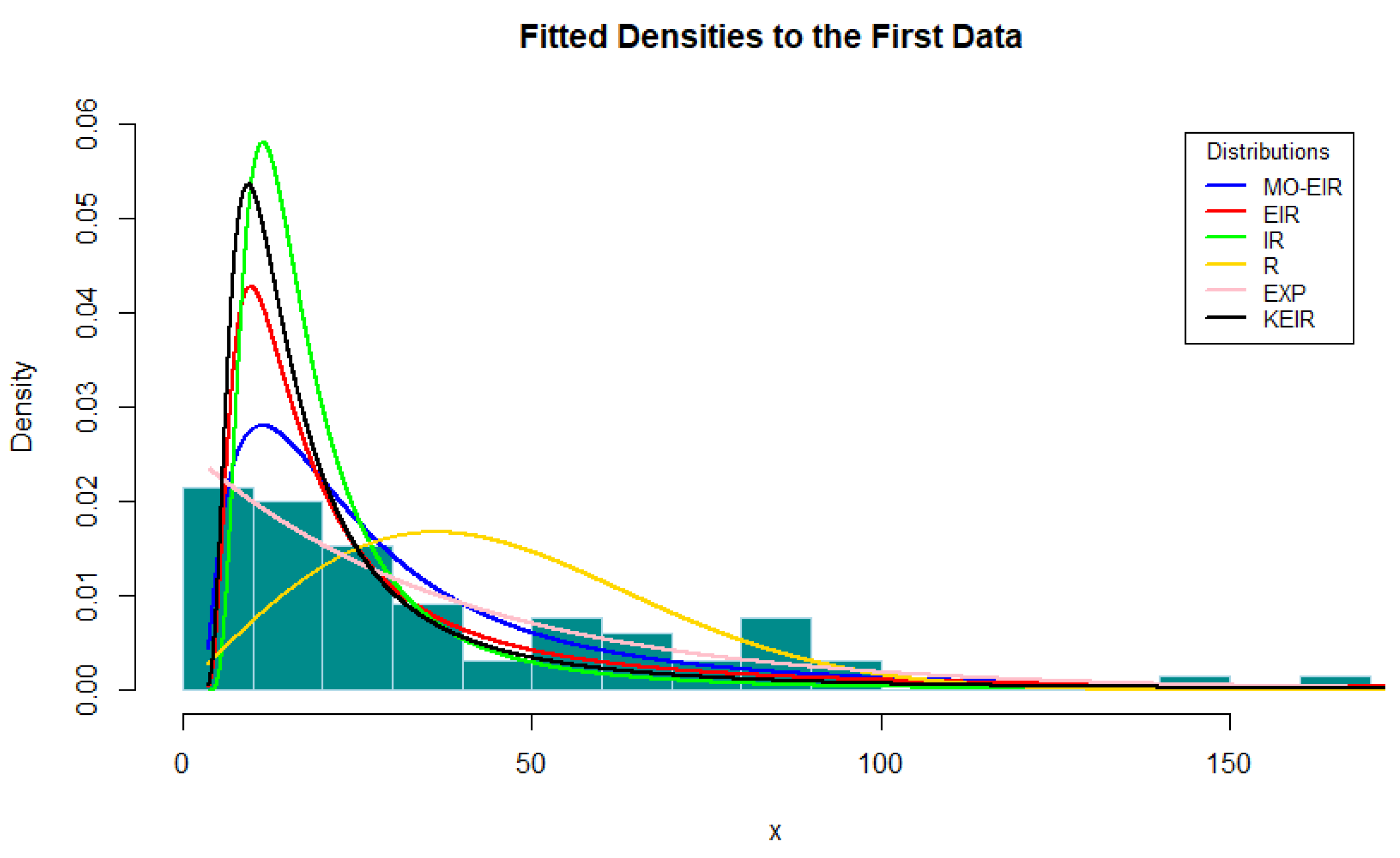
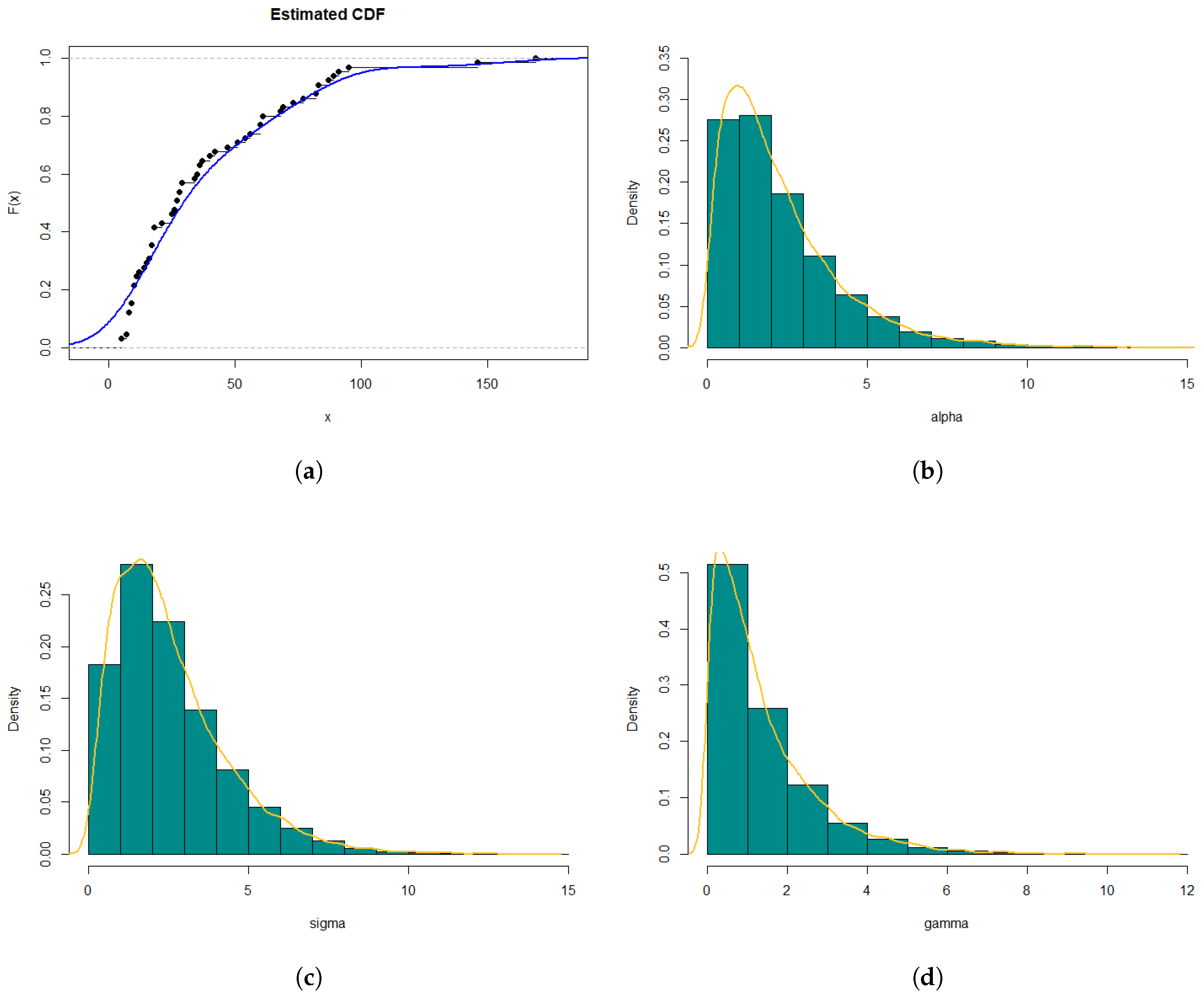
This paper introduces and examines a new generalized form of continuous distributions utilizing the Marshall–Olkin distribution as a foundation. Various significant mathematical properties are deduced, encompassing moments, the moment generating function, order statistics, entropy, and quantile function. Two distinct estimation approaches, namely, maximum likelihood estimation and Bayesian methods, are investigated. A Monte Carlo simulation is conducted to estimate parameters and scrutinize the behavior of the proposed distribution. Bayesian estimation is achieved through the Gibbs sampler and Metropolis–Hastings algorithm which show superb performance. Finally, the new distribution is applied to two real-world datasets, demonstrating the practical utility of the M-O-EIR distribution. It is determined that the M-O-EIR offers superior fits compared to other competitive distributions for these specific datasets. Furthermore, the effectiveness of the ML estimation is contrasted with the Bayesian method on the same dataset, revealing that the Bayesian method outperforms the ML estimation method. Future research could explore improving the proposed distribution by considering alternative baseline distributions within the Marshall–Olkin framework. Additionally, the model may be extended to incorporate other parameter-estimation techniques, such as L-moments and least squares estimation.