Porous and Magnetic Effects on Axial Couette Flows of Second Grade Fluids in Cylindrical Domains

Abstract

Axial Couette flows of electrically conducting incompressible second grade fluids are analytically and numerically investigated through a porous medium in the presence of a constant magnetic field. General exact analytical expressions are derived for the dimensionless velocities corresponding to unidirectional unsteady motions in an infinite circular cylinder and between two infinite coaxial circular cylinders. They can be immediately particularized to give similar results for Newtonian fluids in same flows. Exact expressions for steady velocities of a large class of flows were provided. Due to the generality of boundary conditions the problems in discussion are completely solved. For illustration, some case studies with engineering applications are considered and the corresponding velocity fields are provided. Their correctness is graphically proved. It was also proved that the fluid flows slower and the steady state is rather touched in the presence of a magnetic field or porous medium. Moreover, the steady state is rather touched in the case of the motions between circular coaxial cylinders as compared with same motions in an infinite circular cylinder.

1. Introduction

Flows of incompressible second grade fluids have been extensively investigated in the existing literature. Ting [1] was among the first authors who derived exact solutions for motions of such fluids both in rectangular and cylindrical domains. Other important studies regarding isothermal flows of these fluids in cylindrical domains have been offered by Rajagopal [2], Bandelli and Rajagopal [3], Fetecacau and Corina Fetecau [4], Erdogan and Imrak [5] and Bano et al. [6]. Exact general solutions for unsteady unidirectional motions of same fluids induced by an infinite circular cylinder that applies longitudinal or rotational shear stresses to the fluid have been established by Corina Fetecau et al. [7]. The natural convection of these fluids in an oscillating circular cylinder has been recently investigated by Maria Javaid et al. [8]. Interesting results concerning unsteady flows of incompressible second grade fluids in rectangular domains were obtained, for instance, by Erdogan [9], Erdogan and Imrak [10], Yao and Liu [11], Sultan et al. [12], Imran et al. [13], Baranovskii and Artemov [14], Veera Krishna and Subba Reddy [15], Fetecau and Vieru [16], Baranovskii [17] and Kanuri et al. [18].

It is also known that the motion of a fluid through a porous medium or in the presence of a magnetic field has many engineering applications. Motions through porous media have practical applications in geophysics, astrophysics, composite manufacturing processes, oil reservoir technology, the petroleum industry and agriculture. Interaction between a moving electrically conducting fluid and a magnetic field generates effects that have multiple applications in physics, chemistry and engineering. However, in the existing literature, are few results regarding flows of electrically conducting incompressible second grade fluids (ECISGFs) in cylindrical domains under the influence of a magnetic field or porous medium. Jamil and Zafarullah [19] provided interesting exact solutions for some magnetohydrodynamic (MHD) motions of such fluids between circular cylinders when porous effects are taken into consideration. Unfortunately, their work contains some writing mistakes (see Eqs. (9) and (19), for instance) and it does not contain any proof of the results’ correctness. General solutions for some MHD rotational motions of ECISGFs through a porous medium in an infinite circular cylinder have been recently established by Fetecau et al. [20].

The main purpose of this work is to study axial Couette flows of ECISGFs through a porous medium in cylindrical domains under the influence of a magnetic field. Exact general expressions are derived for the dimensionless velocity fields of the fluid motion induced by an infinite circular cylinder that moves along its symmetry axis with a time-dependent velocity. Actually, they represent the first general solutions for such flows of ECISGFs in cylindrical domains and are obtained in the simplest way using the finite Hankel transform only. For the results validation, as well as to bring to light the fluid behavior in some concrete situations, three particular cases are considered and the corresponding velocity fields are provided. They are written as sum of steady state and transient components. The steady state components of these velocities are presented in two different forms whose equivalency is graphically proved. Graphical representations clearly show that the fluid flows faster and the steady state comes later in the absence of a magnetic field or porous medium.

2. Problem Presentation

Let us consider an ECISGF at rest in a porous medium in an infinite circular cylinder of radius R or between two infinite coaxial circular cylinders of radii $R_1$ and $R_2(>R_1)$. Its constitutive equation is given by the relation

$$\mathit{T}=-p\mathit{I}+\mu {\mathit{A}}_1+{\alpha }_1{\mathit{A}}_2+{\alpha }_2{\mathit{A}}_1^2,$$

(1)

in which T is the stress tensor, ${\mathit{A}}_1$ and ${\mathit{A}}_2$ are the first two Rivlin-Ericksen tensors, I is the unit tensor, p is the hydrostatic pressure, $\mu$ is the dynamic viscosity of the fluid, while ${\alpha }_1$ and ${\alpha }_2$ are material constants. Taking ${\alpha }_1={\alpha }_2=0$ in Equation (1), the governing equation of incompressible Newtonian fluids is obtained.

At the moment $t=0^{+}$ the cylinder in the first case or the outer cylinder in the second case begins to slide along its symmetry axis with the velocity $Vf(t)$ and a circular magnetic field of constant strength B acts in the azimuthally direction on the fluid motion [19,21]. The function $f(\cdot )$ is piecewise continuous and has the zero value in $t=0$ while V is a constant velocity. Owing to the shear the fluid begins to move and, bearing in mind the previous results in the field, we are looking for a velocity field whose velocity vector v is given by the relation

$$\mathit{v}=\mathit{v}(r,t)=v(r,t)\mathit{k},$$

(2)

reported to a convenient cylindrical coordinate system r, $\theta$ and z in which k is the unit vector along z-direction. Introducing v from Equation (2) in (1) one obtains the relation

$$\tau (r,t)=\left(\mu +{\alpha }_1{\displaystyle \frac{\partial }{\partial t}}\right){\displaystyle \frac{\partial v(r,t)}{\partial r}}.$$

(3)

for the non-trivial shear stress $\tau (r,t)=T_{rz}(r,t)$.

In the next we assume that the fluid is finitely conducting, its magnetic permeability is constant, the induced magnetic field is negligible and there is no surplus electric charge distribution. In these conditions, in absence of a pressure gradient in the flow direction, the balance of linear momentum reduces to the differential equation (see [19])

$$\rho {\displaystyle \frac{\partial v(r,t)}{\partial t}}={\displaystyle \frac{\partial \tau (r,t)}{\partial r}}+{\displaystyle \frac{1}{r}}\tau (r,t)-\sigma B^{2}v(r,t)-{\displaystyle \frac{\phi }{k}}\left(\mu +{\alpha }_1{\displaystyle \frac{\partial }{\partial t}}\right) v(r,t),$$

(4)

where $\rho$ is the fluid density, $\sigma$ is the electrical conductivity while $\phi$ and k are the porosity and the permeability of the porous medium. Replacing $\tau (r,t)$ from Equation (3) in (4) one finds the governing equation [19,21]

$$\rho {\displaystyle \frac{\partial v(r,t)}{\partial t}}=\left(\mu +{\alpha }_1{\displaystyle \frac{\partial }{\partial t}}\right)\left[{\displaystyle \frac{{\partial }^{2}v(r,t)}{\partial r^2}}+{\displaystyle \frac{1}{r}}{\displaystyle \frac{\partial v(r,t)}{\partial r}}\right]-\sigma B^{2}v(r,t)-{\displaystyle \frac{\phi }{k}}\left(\mu +{\alpha }_1{\displaystyle \frac{\partial }{\partial t}}\right)v(r,t),$$

(5)

for the velocity field $v(r,t)$. The corresponding initial and boundary conditions are

$$v(r,0)=0,\hspace{0.17em}\hspace{0.17em}\hspace{0.17em}0\le r\le R;\hspace{0.17em}\hspace{0.17em}\hspace{0.17em}v(R,t)=Vf(t),\hspace{0.17em}\hspace{0.17em}\hspace{0.17em}t>0,$$

(6)

for motions in an infinite circular cylinder.

3. Fluid Velocity for Flows Through a Circular Cylinder

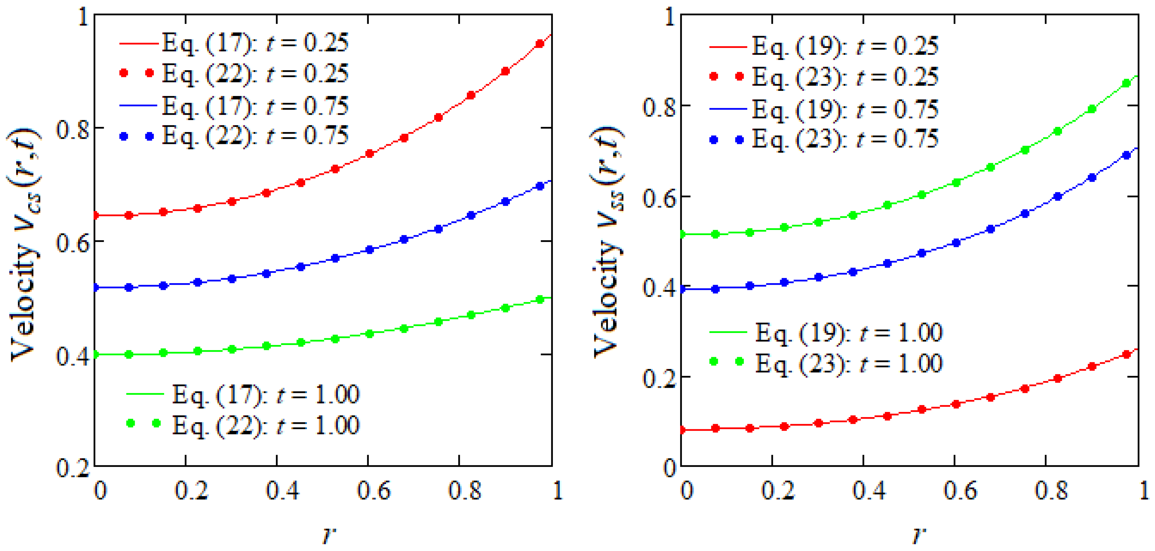
In order to determine the velocity field corresponding to this flow, the governing Equation (5) together with the initial and boundary conditions (6) has to be solved. Using the next non-dimensional functions and variables

$$r^{\ast }={\displaystyle \frac{1}{R}}r,\hspace{0.17em}\hspace{0.17em}\hspace{0.17em}{t}^{\ast }={\displaystyle \frac{\nu }{R^2}}t,\hspace{0.17em}\hspace{0.17em}\hspace{0.17em}{v}^{\ast }={\displaystyle \frac{1}{V}}v,\hspace{0.17em}\hspace{0.17em}\hspace{0.17em}{\tau }^{\ast }={\displaystyle \frac{R}{\mu V}}\tau ,\hspace{0.17em}\hspace{0.17em}\hspace{0.17em}{f}^{\ast }(t^{\ast })=f\left({\displaystyle \frac{R^2}{\nu }}{t}^{\ast }\right),$$

(7)

one attains to the next initial-boundary value problem

$${\displaystyle \frac{\partial v(r,t)}{\partial t}}=\left(1+\alpha {\displaystyle \frac{\partial }{\partial t}}\right)\left[{\displaystyle \frac{{\partial }^{2}v(r,t)}{\partial r^2}}+{\displaystyle \frac{1}{r}}{\displaystyle \frac{\partial v(r,t)}{\partial r}}\right]-Mv(r,t)-K\left(1+\alpha {\displaystyle \frac{\partial }{\partial t}}\right)v(r,t),$$

(8)

$$v(r,0)=0,\hspace{0.17em}\hspace{0.17em}\hspace{0.17em}0\le r\le 1;\hspace{1em}v(1,t)=f(t),\hspace{0.17em}\hspace{0.17em}\hspace{0.17em}t>0.$$

(9)

The constant $\alpha$ and the magnetic and porous parameters M and K, respectively, from Equation (8) are defined by the relations

$$\alpha ={\displaystyle \frac{{\alpha }_1}{\rho R^2}},\hspace{0.17em}\hspace{0.17em}\hspace{0.17em}M={\displaystyle \frac{R^2}{\mu }}\sigma B^2={\displaystyle \frac{R^2}{\nu }}{\displaystyle \frac{\sigma B^2}{\rho }},\hspace{0.17em}\hspace{0.17em}\hspace{0.17em}K={\displaystyle \frac{\phi }{k}}{R}^2.$$

(10)

The magnetic parameter M is an important indicator of the influence of the magnetic field on the fluid flow. It represents the ratio between the electromagnetic forces and the inertial forces in the fluid. The non-dimensional form of Equation (3) is

$$\tau (r,t)=\left(1+\alpha {\displaystyle \frac{\partial }{\partial t}}\right){\displaystyle \frac{\partial v(r,t)}{\partial r}};\hspace{0.17em}\hspace{0.17em}\hspace{0.17em}\hspace{0.17em}0<r<1,\hspace{0.17em}\hspace{0.17em}\hspace{0.17em}t>0.$$

(11)

To determine the dimensionless velocity field $v(r,t)$ corresponding to the motions in discussion, the finite Hankel transform and its inverse defined by the relations (A1) from Appendix A and the identity (A2) are used. In these relations $J_0(\cdot )$ and $J_1(\cdot )$ are Bessel functions of the first kind of zero and one order, respectively, and $r_n$ are the positive roots of the transcendental equation $J_0(r)=0$. Consequently, multiplying Equation (8) by $r{J}_0(r{r}_n)$, integrating the result between 0 and 1 one finds

$${\displaystyle \frac{\partial v_H(r_n,t)}{\partial t}}+{\displaystyle \frac{r_n^2+K_{eff}}{1+\alpha (r_n^2+K)}}{v}_H(r_n,t)-{\displaystyle \frac{f(t)+\alpha f^{\prime }(t)}{1+\alpha (r_n^2+K)}}{r}_n{J}_1(r_n)=0,\hspace{0.17em}\hspace{0.17em}\hspace{0.17em}{v}_H(r_n,0)=0.$$

(12)

In above relation $K_{eff}=M+K$ is the effective permeability. The solution of the problem with initial value (12) is given by the relation

$$\begin{array}{l}{v}_H(r_n,t)=\alpha f(t){\displaystyle \frac{r_n{J}_1(r_n)}{1+\alpha (r_n^2+K)}}\\ +(1-\alpha M){\displaystyle \frac{r_n{J}_1(r_n)}{{[1+\alpha (r_n^2+K)]}^2}}{\displaystyle \underset{0}{\overset{t}{\int }}f(s)}\exp \left[-{\displaystyle \frac{r_n^2+K_{eff}}{1+\alpha (r_n^2+K)}}(t-s)\right]ds.\end{array}$$

(13)

Applying the inverse finite Hankel transform to Equality (13) and using the first entry of Table X from Appendix C of the reference [22] one finds that the dimensionless starting velocity $v(r,t)$ of the fluid can be written in the suitable form

$$\begin{array}{l}v(r,t)=f(t)-2(1+\alpha K)f(t){\displaystyle \sum _{n=1}^{\infty }\frac{J_0(r{r}_n)}{[1+\alpha (r_n^2+K)]r_n{J}_1(r_n)}}\\ +2(1-\alpha M){\displaystyle \sum _{n=1}^{\infty }\frac{r_n{J}_0(r{r}_n)}{{[1+\alpha (r_n^2+K)]}^2{J}_1(r_n)}}{\displaystyle \underset{0}{\overset{t}{\int }}f(s)}\exp \left[-{\displaystyle \frac{r_n^2+K_{eff}}{1+\alpha (r_n^2+K)}}(t-s)\right]ds,\end{array}$$

(14)

which satisfies the initial and boundary conditions (9). In above relations $J_0(\cdot )$ and $J_1(\cdot )$ are standard Bessel functions of the first kind of zero and one order, respectively.

Making $\alpha =0$ in Equation (14) one finds the dimensionless starting velocity field

$$v_N(r,t)=f(t)-2f(t){\displaystyle \sum _{n=1}^{\infty }\frac{J_0(r{r}_n)}{r_n{J}_1(r_n)}}+2{\displaystyle \sum _{n=1}^{\infty }\frac{r_n{J}_0(r{r}_n)}{J_1(r_n)}}{\displaystyle \underset{0}{\overset{t}{\int }}f(s)}{\mathrm{e}}^{-(r_n^2+K_{eff})(t-s)}ds,$$

(15)

corresponding to MHD axial Couette flow of electrically conducting incompressible Newtonian fluids through a porous medium in an infinite circular cylinder that moves along its symmetry axis with the velocity $Vf(t)$. This velocity does not depend of the parameters M and K independently and a two parameter approach in this case is superfluous. The dimensionless starting shear stresses $\tau (r,t)$ and ${\tau }_N(r,t)$ corresponding to the same motion of incompressible second grade and Newtonian fluids can be immediately obtained substituting $v(r,t)$ and $v_N(r,t)$ from Equations (14) and (15) in (11).

The relation (14) gives the general expression of the dimensionless velocity field $v(r,t)$ corresponding to MHD axial Couette flow of ECISGFs through a porous medium in an infinite circular cylinder that moves along its symmetry axis with the time dependent velocity $Vf(t)$. Using this expression it is possible to derive the velocity field for any motion of this kind of the respective fluids. Consequently, the problem in discussion is completely solved. For illustration, some particular study cases are considered in the following and the corresponding velocity fields are provided. They will be later used to bring to light some characteristics of the fluid motion and to find the necessary time to reach the steady state. This time is very important for experimental researchers who want to know the transition moment of the motion to the steady or permanent sate.

3.1. Case $f(t)=H(t)\cos (\omega t)$ or $f(t)=H(t)\sin (\omega t)$ (Motion in a Cylinder)

Replacing $f(t)$ by $H(t)\cos (\omega t)$ or $H(t)\sin (\omega t)$ in Equation (14) (where $H(t)$ is the Heaviside unit step function and $\omega$ is the non-dimensional frequency of the oscillations) one finds the dimensionless starting velocity fields $v_c(r,t)$ and $v_s(r,t)$ corresponding to the axial Couette flows induced by cosine or sine oscillations, respectively, of the cylinder along its symmetry axis. Since these flows become steady in time, the corresponding starting velocities can be written as sum of their steady state (long time) and transient components, i.e.,

$$v_c(r,t)=[v_{cs}(r,t)+v_{ct}(r,t)]H(t),\hspace{1em}{v}_s(r,t)=[v_{ss}(r,t)+v_{st}(r,t)]H(t),$$

(16)

where

$$\begin{array}{l}{v}_{cs}(r,t)=\cos (\omega t)-2(1+\alpha K)\cos (\omega t){\displaystyle \sum _{n=1}^{\infty }\frac{J_0(r{r}_n)}{[1+\alpha (r_n^2+K)]r_n{J}_1(r_n)}}\\ +2(1-\alpha M)\cos (\omega t){\displaystyle \sum _{n=1}^{\infty }\frac{r_n(r_n^2+K_{eff})J_0(r{r}_n)}{[1+\alpha (r_n^2+K)]a_n{J}_1(r_n)}}+2\omega (1-\alpha M)\sin (\omega t){\displaystyle \sum _{n=1}^{\infty }\frac{r_n{J}_0(r{r}_n)}{a_n{J}_1(r_n)}},\end{array}$$

(17)

$$v_{ct}(r,t)=-2(1-\alpha M){\displaystyle \sum _{n=1}^{\infty }\frac{r_n(r_n^2+K_{eff})J_0(r{r}_n)}{[1+\alpha (r_n^2+K)]a_n{J}_1(r_n)}}\exp \left[-{\displaystyle \frac{r_n^2+K_{eff}}{1+\alpha (r_n^2+K)}}t\right],$$

(18)

$$\begin{array}{l}{v}_{ss}(r,t)=\sin (\omega t)-2(1+\alpha K)\sin (\omega t){\displaystyle \sum _{n=1}^{\infty }\frac{J_0(r{r}_n)}{[1+\alpha (r_n^2+K)]r_n{J}_1(r_n)}}\\ +2(1-\alpha M)\sin (\omega t){\displaystyle \sum _{n=1}^{\infty }\frac{r_n(r_n^2+K_{eff})J_0(r{r}_n)}{[1+\alpha (r_n^2+K)]a_n{J}_1(r_n)}}-2\omega (1-\alpha M)\cos (\omega t){\displaystyle \sum _{n=1}^{\infty }\frac{r_n{J}_0(r{r}_n)}{a_n{J}_1(r_n)}},\end{array}$$

(19)

$$v_{st}(r,t)=2\omega (1-\alpha M){\displaystyle \sum _{n=1}^{\infty }\frac{r_n{J}_0(r{r}_n)}{a_n{J}_1(r_n)}}\exp \left[-{\displaystyle \frac{r_n^2+K_{eff}}{1+\alpha (r_n^2+K)}}t\right].$$

(20)

The constants $a_n$ from the above relations are given by the relation

$$a_n={(r_n^2+K_{eff})}^2+{\omega }^2{[1+\alpha (r_n^2+K)]}^2, n=1,2,3\dots$$

(21)

For a check of the obtained results, let us provide equivalent expressions for the steady state velocities $v_{cs}(r,t)$ and $v_{ss}(r,t)$, namely

$$v_{cs}(r,t)=\mathrm{Re}\left\{{\displaystyle \frac{I_0(r\sqrt{\gamma })}{I_0(\sqrt{\gamma })}}{\mathrm{e}}^{i\omega t}\right\},$$

(22)

$$v_{ss}(r,t)=\mathrm{Im}\left\{{\displaystyle \frac{I_0(r\sqrt{\gamma })}{I_0(\sqrt{\gamma })}}{\mathrm{e}}^{i\omega t}\right\},$$

(23)

where Re and Im mean the real part and the imaginary part of that which follows. The complex constant $\gamma$ from these expressions, that have been determined using the complex velocity $v_{com}(r,t)=v_{cs}(r,t)+i{v}_{ss}(r,t)$, is given by the relation

$$\gamma ={\displaystyle \frac{K_{eff}+i\omega (1+\alpha K)}{1+i\omega \alpha }}$$

(24)

and Figure 1 shows the equivalence of the expressions of $v_{cs}(r,t)$ and $v_{ss}(r,t)$ given by the relations (17), (22) and (19), (23), respectively. Of course, in the case of incompressible Newtonian fluids, all previous relations take simpler forms. The steady state velocities from Equations (22) and (23), for instance, become

$$v_{cs}(r,t)=\mathrm{Re}\left\{{\displaystyle \frac{I_0(r\sqrt{K_{eff}+i\omega })}{I_0(\sqrt{K_{eff}+i\omega })}}{\mathrm{e}}^{i\omega t}\right\},\hspace{0.17em}\hspace{0.17em}\hspace{0.17em}\hspace{0.17em}{v}_{ss}(r,t)=\mathrm{Im}\left\{{\displaystyle \frac{I_0(r\sqrt{K_{eff}+i\omega })}{I_0(\sqrt{K_{eff}+i\omega })}}{\mathrm{e}}^{i\omega t}\right\}.$$

(25)

In above relations $I_0(\cdot )$ is the modified Bessel function of the first kind of zero order.

3.2. Case $f(t)=H(t)$ (Motion in a Cylinder)

In this case the fluid motion is generated by the cylinder that slides along its symmetry axis with the constant velocity V. The expressions of steady and transient components $v_{Cs}(r)$ and $v_{Ct}(r,t)$ of the corresponding starting velocity $v_C(r,t)$, namely

$$v_{Cs}(r)=1-2K_{eff}{\displaystyle \sum _{n=1}^{\infty }\frac{J_0(r{r}_n)}{r_n(r_n^2+K_{eff})J_1(r_n)}},$$

(26)

$$v_{Ct}(r,t)=-2(1-\alpha M){\displaystyle \sum _{n=1}^{\infty }\frac{r_n{J}_0(r{r}_n)}{[1+\alpha (r_n^2+K)](r_n^2+K_{eff})J_1(r_n)}}\exp \left[-{\displaystyle \frac{r_n^2+K_{eff}}{1+\alpha (r_n^2+K)}}t\right],$$

(27)

have been directly obtained putting $\omega =0$ in Equations (17) and (18). An equivalent expression for the dimensionless steady velocity $v_{Cs}(r)$, namely

$$v_{Cs}(r)={\displaystyle \frac{I_0(r\sqrt{K_{eff}})}{I_0(\sqrt{K_{eff}})}},$$

(28)

has been derived from Equation (22).

3.3. Case When $\underset{t\to \infty }{\lim }f(t)=\mathcal{l}<\infty$

It is interesting to observe that the steady velocity field corresponding to such a motion can be generally determined using the following property

$$\underset{s\to 0}{\lim }s\overline{g}(s)=\underset{t\to \infty }{\lim }g(t),$$

(29)

if $\overline{g}(s)$ is the Laplace transform of $g(t)$. Indeed, applying the Laplace transform to the equality (14) one finds that

$$\begin{array}{l}\overline{v}(r,s)=\overline{f}(s)-2(1+\alpha K)\overline{f}(s){\displaystyle \sum _{n=1}^{\infty }\frac{J_0(r{r}_n)}{[1+\alpha (r_n^2+K)]r_n{J}_1(r_n)}}\\ +2(1-\alpha M)\overline{f}(s){\displaystyle \sum _{n=1}^{\infty }\frac{r_n{J}_0(r{r}_n)}{{[1+\alpha (r_n^2+K)]}^2{J}_1(r_n)}}\overline{f}(s){\displaystyle \frac{1}{s+\frac{r_n^2+K_{eff}}{1+\alpha (r_n^2+K)}}}.\end{array}$$

(30)

Multiplying the equality (30) with s, taking its limit when $s\to 0$ and bearing in mind the property (29) one finds the steady or permanent velocity field

$$v_p(r)=\mathcal{l}-2\mathcal{l}{K}_{eff}{\displaystyle \sum _{n=1}^{\infty }\frac{J_0(r{r}_n)}{r_n(r_n^2+K_{eff})J_1(r_n)}}.$$

(31)

Now, taking $\mathcal{l}=1$ in the last equality one recovers $v_{Cs}(r)$ from Equality (26).

4. Fluid Velocity for Flows Between Infinite Coaxial Circular Cylinders

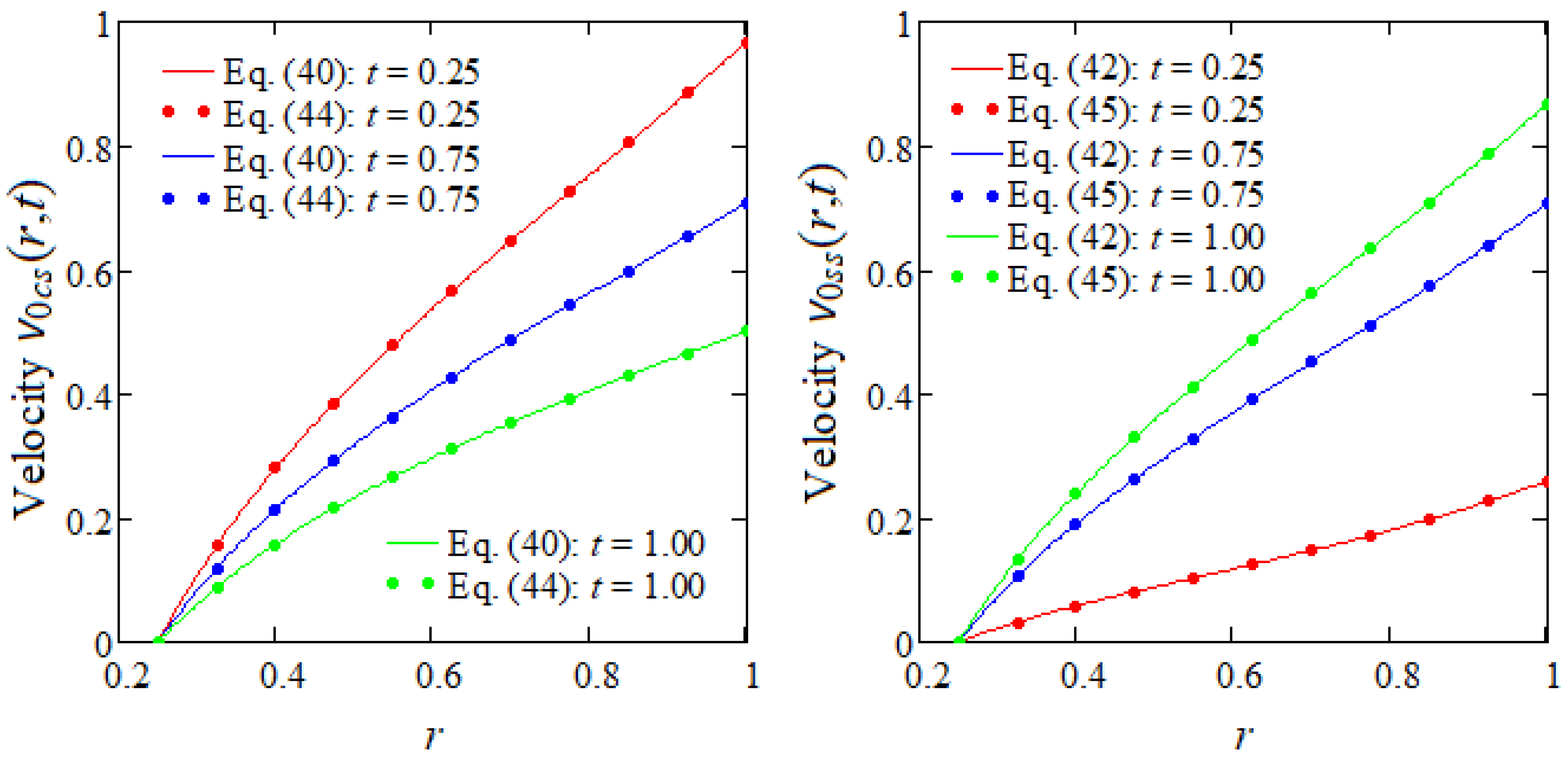
The initial and boundary conditions for this motion are

$$v(r,0)=0,\hspace{0.17em}\hspace{0.17em}\hspace{0.17em}{R}_1\le r\le R_2;\hspace{0.17em}\hspace{0.17em}\hspace{0.17em}v(R_1,t)=0,\hspace{0.17em}\hspace{0.17em}\hspace{0.17em}v(R_2,t)=Vf(t),\hspace{0.17em}\hspace{0.17em}\hspace{0.17em}t>0.$$

(32)

Introducing the next non-dimensional variables and functions

$$r^{\ast }={\displaystyle \frac{1}{R_2}}r,\hspace{0.17em}\hspace{0.17em}\hspace{0.17em}{t}^{\ast }={\displaystyle \frac{\nu }{R_2^2}}t,\hspace{0.17em}\hspace{0.17em}\hspace{0.17em}{v}^{\ast }={\displaystyle \frac{1}{V}}v,\hspace{0.17em}\hspace{0.17em}\hspace{0.17em}{\tau }^{\ast }={\displaystyle \frac{R_2}{\mu V}}\tau ,\hspace{0.17em}\hspace{0.17em}\hspace{0.17em}{f}^{\ast }(t^{\ast })=f\left({\displaystyle \frac{R_2^2}{\nu }}{t}^{\ast }\right),$$

(33)

and again dropping out the star notation one obtains the same dimensionless form (8) for the governing equation of the dimensionless velocity field $v(r,t)$. The corresponding initial and boundary conditions are

$$v(r,0)=0,\hspace{0.17em}\hspace{0.17em}\hspace{0.17em}{r}_0\le r\le 1;\hspace{1em}v(r_0,t)=0,\hspace{0.17em}\hspace{0.17em}\hspace{0.17em}v(1,t)=f(t),\hspace{0.17em}\hspace{0.17em}\hspace{0.17em}t>0,$$

(34)

where the constant $r_0=R_1/R_2$.

In order to solve the partial differential Equation (8) with the initial and boundary conditions (34), we use the finite Hankel transform and its inverse defined by the relations (A3) from Appendix A [23]. Multiplying Equation (8) by $rA(r,r_n)$ where $r_n$ are the positive roots of the transcendental equation $A(1,r)=0$ and

$$A(r,r_n)=Y_0(r_0{r}_n)J_0(r{r}_n)-J_0(r_0{r}_n)Y_0(r{r}_n)$$

(35)

and integrating the result between the limits $r_0$ and 1 and bearing in mind the identity (A4) from Appendix A one finds the following problem with initial value

$${\displaystyle \frac{\partial v_{H0}(r_n,t)}{\partial t}}+{\displaystyle \frac{r_n^2+K_{eff}}{1+\alpha (r_n^2+K)}}{v}_{H0}(r_n,t)={\displaystyle \frac{2}{\pi }}{\displaystyle \frac{f(t)+\alpha f^{\prime }(t)}{1+\alpha (r_n^2+K)}}{\displaystyle \frac{J_0(r_0{r}_n)}{J_0(r_n)}},\hspace{0.17em}\hspace{0.17em}\hspace{0.17em}{v}_{H0}(r_n,0)=0.$$

(36)

The solution of this problem is given by the relation

$$\begin{array}{l}{v}_{H0}(r_n,t)={\displaystyle \frac{2}{\pi }}{\displaystyle \frac{\alpha f(t)J_0(r_0{r}_n)}{[1+\alpha (r_n^2+K)]J_0(r_n)}}\\ +{\displaystyle \frac{2(1-\alpha M)J_0(r_0{r}_n)}{\pi J_0(r_n){[1+\alpha (r_n^2+K)]}^2}}{\displaystyle \underset{0}{\overset{t}{\int }}f(s)}\exp \left[-{\displaystyle \frac{r_n^2+K_{eff}}{1+\alpha (r_n^2+K)}}(t-s)\right]ds.\end{array}$$

(37)

Applying the inverse finite Hankel transform to the last relation, one finds the dimensionless velocity field

$$\begin{array}{l}{v}_0(r,t)=\alpha \pi f(t){\displaystyle \sum _{n=1}^{\infty }\frac{r_n^2{J}_0(r_0{r}_n)J_0(r_n)A(r,r_n)}{[1+\alpha (r_n^2+K)][J_0^2(r_0{r}_n)-J_0^2(r_n)]}}+\pi (1-\alpha M)\\ \times {\displaystyle \sum _{n=1}^{\infty }\frac{r_n^2{J}_0(r_0{r}_n)J_0(r_n)A(r,r_n)}{{[1+\alpha (r_n^2+K)]}^2[J_0^2(r_0{r}_n)-J_0^2(r_n)]}}{\displaystyle \underset{0}{\overset{t}{\int }}f(s)}\exp \left[-{\displaystyle \frac{r_n^2+K_{eff}}{1+\alpha (r_n^2+K)}}(t-s)\right]ds.\end{array}$$

(38)

In this form, the dimensionless velocity $v_0(r,t)$ satisfies the initial condition and the first boundary condition. The second boundary condition seems to be unsatisfied. An equivalent form for the velocity field $v_0(r,t)$, namely

$$\begin{array}{l}{v}_0(r,t)={\displaystyle \frac{r^2-r_0^2}{1-r_0^2}}f(t)-\pi (1+\alpha K)f(t){\displaystyle \sum _{n=1}^{\infty }\frac{J_0(r_0{r}_n)J_0(r_n)A(r,r_n)}{[1+\alpha (r_n^2+K)][J_0^2(r_0{r}_n)-J_0^2(r_n)]}}\\ +{\displaystyle \frac{4\pi f(t)}{1-r_0^2}}{\displaystyle \sum _{n=1}^{\infty }\frac{J_0(r_n)}{r_n^2[J_0(r_0{r}_n)+J_0(r_n)]}}A(r,r_n)+\pi (1-\alpha M)\\ \times {\displaystyle \sum _{n=1}^{\infty }\frac{r_n^2{J}_0(r_0{r}_n)J_0(r_n)A(r,r_n)}{{[1+\alpha (r_n^2+K)]}^2[J_0^2(r_0{r}_n)-J_0^2(r_n)]}}{\displaystyle \underset{0}{\overset{t}{\int }}f(s)}\exp \left[-{\displaystyle \frac{r_n^2+K_{eff}}{1+\alpha (r_n^2+K)}}(t-s)\right]ds,\end{array}$$

(39)

has been obtained using the identities (A5) and (A6) from Appendix A. In this form, $v_0(r,t)$ satisfies all imposed initial and boundary conditions. Taking $\alpha =0$ in Equation (39) one finds the dimensionless velocity field corresponding to the MHD axial Couette flows of electrically conducting incompressible Newtonian fluids through a porous medium induced by the outer cylinder that moves along its symmetry axis with the time dependent velocity $Vf(t)$. Its expression is

$$\begin{array}{l}{v}_{N0}(r,t)={\displaystyle \frac{r^2-r_0^2}{1-r_0^2}}f(t)+{\displaystyle \frac{4\pi f(t)}{1-r_0^2}}{\displaystyle \sum _{n=1}^{\infty }\frac{J_0(r_n)}{r_n^2[J_0(r_0{r}_n)+J_0(r_n)]}}A(r,r_n)\\ -\pi f(t){\displaystyle \sum _{n=1}^{\infty }\frac{J_0(r_0{r}_n)J_0(r_n)A(r,r_n)}{J_0^2(r_0{r}_n)-J_0^2(r_n)}}+\pi {\displaystyle \sum _{n=1}^{\infty }\frac{r_n^2{J}_0(r_0{r}_n)J_0(r_n)A(r,r_n)}{J_0^2(r_0{r}_n)-J_0^2(r_n)}}{\displaystyle \underset{0}{\overset{t}{\int }}f(t-s)}\hspace{0.17em}{\mathrm{e}}^{-(r_n^2+K_{eff})s}ds.\end{array}$$

4.1. Case $f(t)=H(t)\cos (\omega t)$ or $f(t)=H(t)\sin (\omega t)$ (Motion Between Two Cylinders)

Substituting $f(t)$ by $H(t)\cos (\omega t)$ or $H(t)\sin (\omega t)$ in Equation (39) one finds the dimensionless starting velocities $v_{0c}(r,t)$ and $v_{0s}(r,t)$ corresponding to the MHD axial Couette flows of ECISGFs through a porous medium between coaxial circular cylinders due to cosine or sine oscillations, respectively, of the outer cylinder. The dimensionless steady state and transient components $v_{0cs}(r,t),$ $v_{0ct}(r,t)$ and $v_{0ss}(r,t),$ $v_{0st}(r,t)$ of the these velocities, respectively, are given by the relations

$$\begin{array}{l}{v}_{0cs}(r,t)={\displaystyle \frac{r^2-r_0^2}{1-r_0^2}}\cos (\omega t)-\pi (1+\alpha K)\cos (\omega t){\displaystyle \sum _{n=1}^{\infty }\frac{J_0(r_0{r}_n)J_0(r_n)A(r,r_n)}{[1+\alpha (r_n^2+K)][J_0^2(r_0{r}_n)-J_0^2(r_n)]}}\\ +{\displaystyle \frac{4\pi \cos (\omega t)}{1-r_0^2}}{\displaystyle \sum _{n=1}^{\infty }\frac{J_0(r_n)}{r_n^2[J_0(r_0{r}_n)+J_0(r_n)]}}A(r,r_n)+\pi (1-\alpha M)\\ \times {\displaystyle \sum _{n=1}^{\infty }\frac{r_n^2\left[(r_n^2+K_{eff})\cos (\omega t)+\omega [1+\alpha (r_n^2+K)]\sin (\omega t)\right]J_0(r_0{r}_n)J_0(r_n)A(r,r_n)}{[1+\alpha (r_n^2+K)][J_0^2(r_0{r}_n)-J_0^2(r_n)]a_n}},\end{array}$$

(40)

$$v_{0ct}(r,t)=-\pi (1-\alpha M){\displaystyle \sum _{n=1}^{\infty }\frac{r_n^2(r_n^2+K_{eff})J_0(r_0{r}_n)J_0(r_n)A(r,r_n)}{[1+\alpha (r_n^2+K)][J_0^2(r_0{r}_n)-J_0^2(r_n)]a_n}}\exp \left[-{\displaystyle \frac{r_n^2+K_{eff}}{1+\alpha (r_n^2+K)}}t\right],$$

(41)

$$\begin{array}{l}{v}_{0ss}(r,t)={\displaystyle \frac{r^2-r_0^2}{1-r_0^2}}\sin (\omega t)-\pi (1+\alpha K)\sin (\omega t){\displaystyle \sum _{n=1}^{\infty }\frac{J_0(r_0{r}_n)J_0(r_n)A(r,r_n)}{[1+\alpha (r_n^2+K)][J_0^2(r_0{r}_n)-J_0^2(r_n)]}}\\ +{\displaystyle \frac{4\pi \sin (\omega t)}{1-r_0^2}}{\displaystyle \sum _{n=1}^{\infty }\frac{J_0(r_n)}{r_n^2[J_0(r_0{r}_n)+J_0(r_n)]}}A(r,r_n)+\pi (1-\alpha M)\\ \times {\displaystyle \sum _{n=1}^{\infty }\frac{r_n^2\left[(r_n^2+K_{eff})\sin (\omega t)]-\omega [1+\alpha (r_n^2+K)]\cos (\omega t)\right]J_0(r_0{r}_n)J_0(r_n)A(r,r_n)}{[1+\alpha (r_n^2+K)][J_0^2(r_0{r}_n)-J_0^2(r_n)]a_n}},\end{array}$$

(42)

$$v_{0st}(r,t)=\omega \pi (1-\alpha M){\displaystyle \sum _{n=1}^{\infty }\frac{r_n^2{J}_0(r_0{r}_n)J_0(r_n)A(r,r_n)}{[J_0^2(r_0{r}_n)-J_0^2(r_n)]a_n}}\exp \left[-{\displaystyle \frac{r_n^2+K_{eff}}{1+\alpha (r_n^2+K)}}t\right].$$

(43)

Newtonian solutions corresponding to same motions are obtained making $\alpha =0$ in above relations. As before, they do not depend of the magnetic and porous parameters M and K independently, but only by means of the effective permeability $K_{eff}=M+K$.

Equivalent expressions for the steady state velocities $v_{0cs}(r,t)$ and $v_{0ss}(r,t)$ are given by the simple relations

$$v_{0cs}(r,t)=\mathrm{Re}\left\{{\displaystyle \frac{K_0(r_0\sqrt{\gamma })I_0(r\sqrt{\gamma })-I_0(r_0\sqrt{\gamma })K_0(r\sqrt{\gamma })}{K_0(r_0\sqrt{\gamma })I_0(\sqrt{\gamma })-I_0(r_0\sqrt{\gamma })K_0(\sqrt{\gamma })}}{\mathrm{e}}^{i\omega t}\right\},$$

(44)

$$v_{0ss}(r,t)=\mathrm{Im}\left\{{\displaystyle \frac{K_0(r_0\sqrt{\gamma })I_0(r\sqrt{\gamma })-I_0(r_0\sqrt{\gamma })K_0(r\sqrt{\gamma })}{K_0(r_0\sqrt{\gamma })I_0(\sqrt{\gamma })-I_0(r_0\sqrt{\gamma })K_0(\sqrt{\gamma })}}{\mathrm{e}}^{i\omega t}\right\},$$

(45)

where $K_0(\cdot )$ is the modified Bessel function of second kind and zero order. The equivalence of the expressions of the dimensionless steady state velocities fields $v_{0cs}(r,t)$ and $v_{0ss}(r,t)$ given by the relations (40), (44) and (42), (45), respectively, is proved by means of Figure 2.

As it was to be expected, simple computations show that the limits of the steady state velocities $v_{0cs}(r,t)$ and $v_{0ss}(r,t)$ of the motions between infinite circular cylinders give even the steady state velocities $v_{cs}(r,t)$ and $v_{ss}(r,t)$, respectively, of the fluid motions through an infinite circular cylinder when $r_0\to 0$, i.e.,

$$\underset{r_0\to 0}{\lim }{v}_{0cs}(r,t)=\mathrm{Re}\left\{{\displaystyle \frac{I_0(r\sqrt{\gamma })}{I_0(\sqrt{\gamma })}}{\mathrm{e}}^{i\omega t}\right\}=v_{cs}(r,t),$$

(46)

$$\underset{r_0\to 0}{\lim }{v}_{0ss}(r,t)=\mathrm{Im}\left\{{\displaystyle \frac{I_0(r\sqrt{\gamma })}{I_0(\sqrt{\gamma })}}{\mathrm{e}}^{i\omega t}\right\}=v_{ss}(r,t).$$

(47)

For completion, it is showed in Figure 3 that the diagrams of the dimensionless starting velocities fields $v_{0ct}(r,t)$ and $v_{0st}(r,t)$ corresponding to flows between circular cylinders overlap over the diagrams of the starting velocities $v_{ct}(r,t)$ and $v_{st}(r,t)$ of the motions through an infinite circular cylinder when $r_0\to 0$.

4.2. Case $f(t)=H(t)$ (Motion Between Two Cylinders)

Substituting $f(t)$ by H(t) in Equation (39) one finds the dimensionless starting velocity $v_{0C}(r,t)$ corresponding to the motion of ECISGFs between two infinite circular coaxial cylinders induced by the outer cylinder that slides along its symmetry axis with the constant velocity V. The expressions of the steady and transient components $v_{0Cs}(r)$ and $v_{0Ct}(r,t)$ of $v_{0C}(r,t)$, which are given by the relations

$$\begin{array}{l}{v}_{0Cs}(r)={\displaystyle \frac{r^2-r_0^2}{1-r_0^2}}+{\displaystyle \frac{4\pi }{1-r_0^2}}{\displaystyle \sum _{n=1}^{\infty }\frac{J_0(r_n)A(r,r_n)}{r_n^2[J_0(r_0{r}_n)+J_0(r_n)]}}\\ -\pi K_{eff}{\displaystyle \sum _{n=1}^{\infty }\frac{J_0(r_0{r}_n)J_0(r_n)A(r,r_n)}{(r_n^2+K_{eff})][J_0^2(r_0{r}_n)-J_0^2(r_n)]}},\end{array}$$

(48)

$$\begin{array}{l}{v}_{0Ct}(r,t)=-\pi (1-\alpha M){\displaystyle \sum _{n=1}^{\infty }\frac{r_n^2{J}_0(r_0{r}_n)J_0(r_n)A(r,r_n)}{(r_n^2+K_{eff})[1+\alpha (r_n^2+K)][J_0^2(r_0{r}_n)-J_0^2(r_n)]}}\\ \times \exp \left[-{\displaystyle \frac{r_n^2+K_{eff}}{1+\alpha (r_n^2+K)}}t\right],\end{array}$$

(49)

can be directly obtained taking $\omega =0$ in Equations (40) and (41). An equivalent form for the steady component $v_{0Cs}(r)$, namely

$$v_{0Cs}(r)=\mathrm{Re}\left\{{\displaystyle \frac{K_0(r_0\sqrt{K_{eff}})I_0(r\sqrt{K_{eff}})-I_0(r_0\sqrt{K_{eff}})K_0(r\sqrt{K_{eff}})}{K_0(r_0\sqrt{K_{eff}})I_0(\sqrt{K_{eff}})-I_0(r_0\sqrt{K_{eff}})K_0(\sqrt{K_{eff}})}}\right\},$$

(50)

has been obtained replacing $\omega$ by zero in Equation (44). Taking the limit of the equality (50) when $r_0\to 0$ one recovers the velocity field $v_{Cs}(r)$ given by Equation (28). Finally, following the same way as in Section 3.3. and using the expression of $v_{0c}(r,t)$ from Equation (39) with $\omega =0$, it is easily to show that the permanent velocity field $v_{0p}(r)$ corresponding to the case when $\underset{t\to \infty }{\lim }f(t)=\mathcal{l}<\infty$ is given by the simple relation

$$\begin{array}{l}{v}_{0p}(r)={\displaystyle \frac{r^2-r_0^2}{1-r_0^2}}\mathcal{l}+{\displaystyle \frac{4\pi \mathcal{l}}{1-r_0^2}}{\displaystyle \sum _{n=1}^{\infty }\frac{J_0(r_n)}{r_n^2[J_0(r_0{r}_n)+J_0(r_n)]}}A(r,r_n)\\ -\pi \mathcal{l}{K}_{eff}{\displaystyle \sum _{n=1}^{\infty }\frac{J_0(r_0{r}_n)J_0(r_n)}{(r_n^2+K_{eff})][J_0^2(r_0{r}_n)-J_0^2(r_n)]}}A(r,r_n).\end{array}$$

(51)

Making $\mathcal{l}=1$ in above relation one finds the expression of $v_{0Cs}(r)$ from Equation (48).

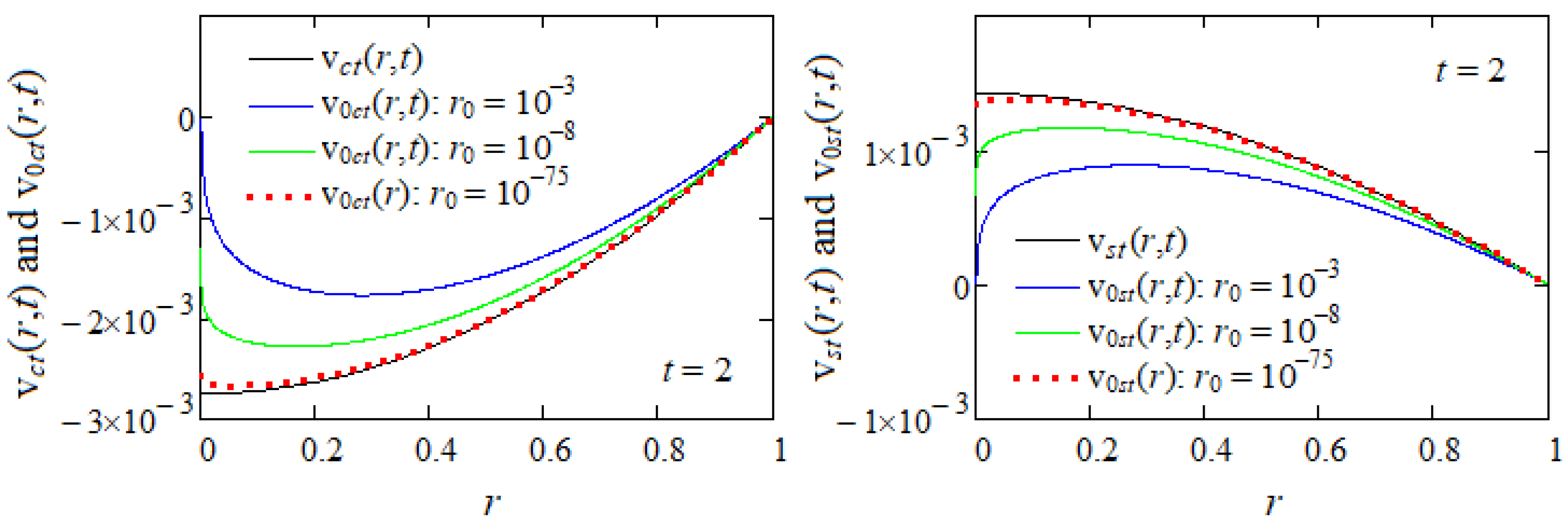
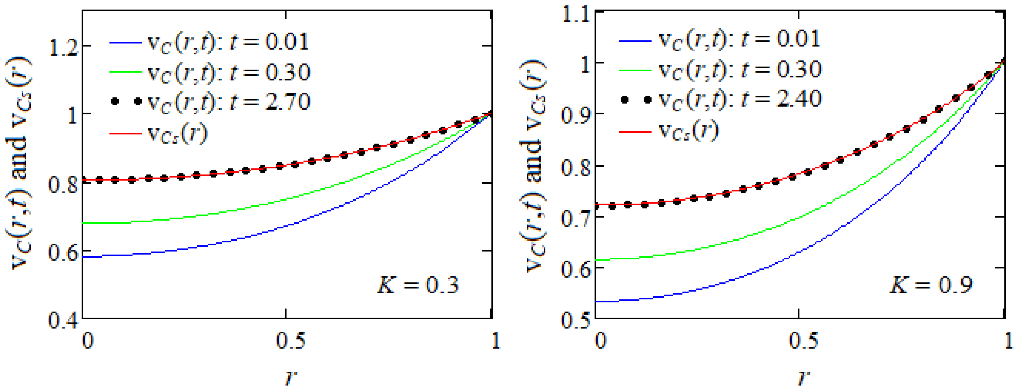
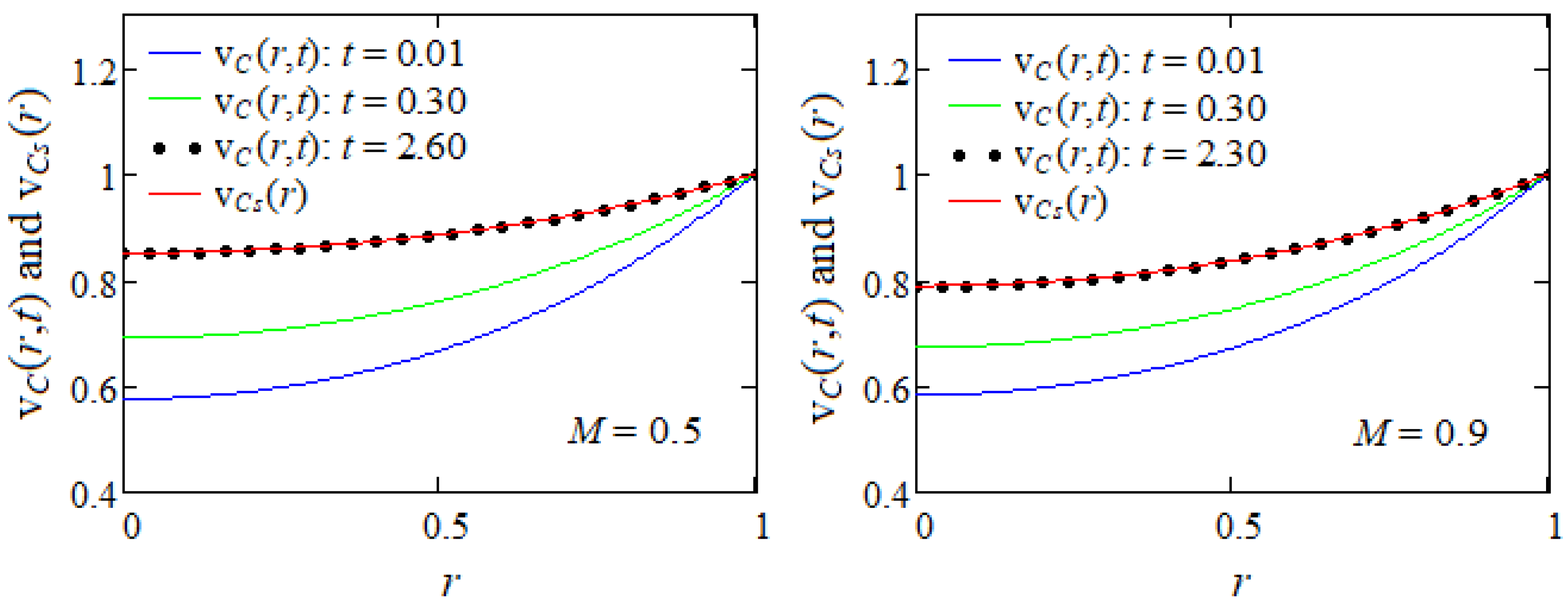
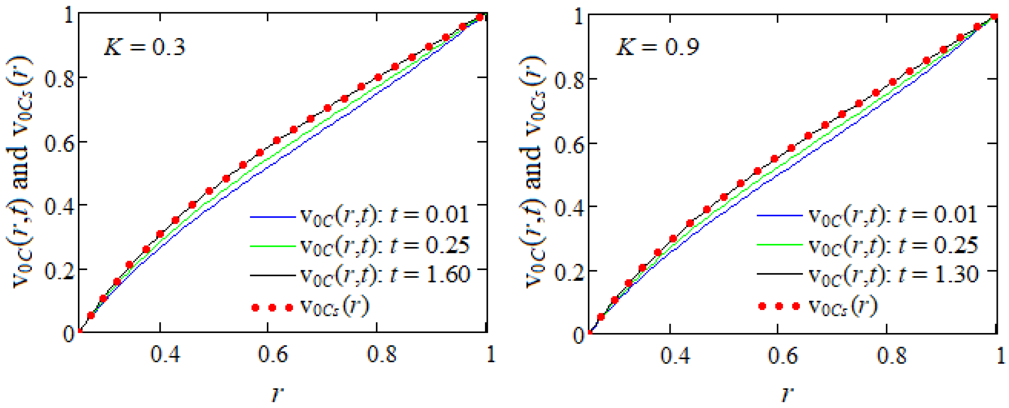
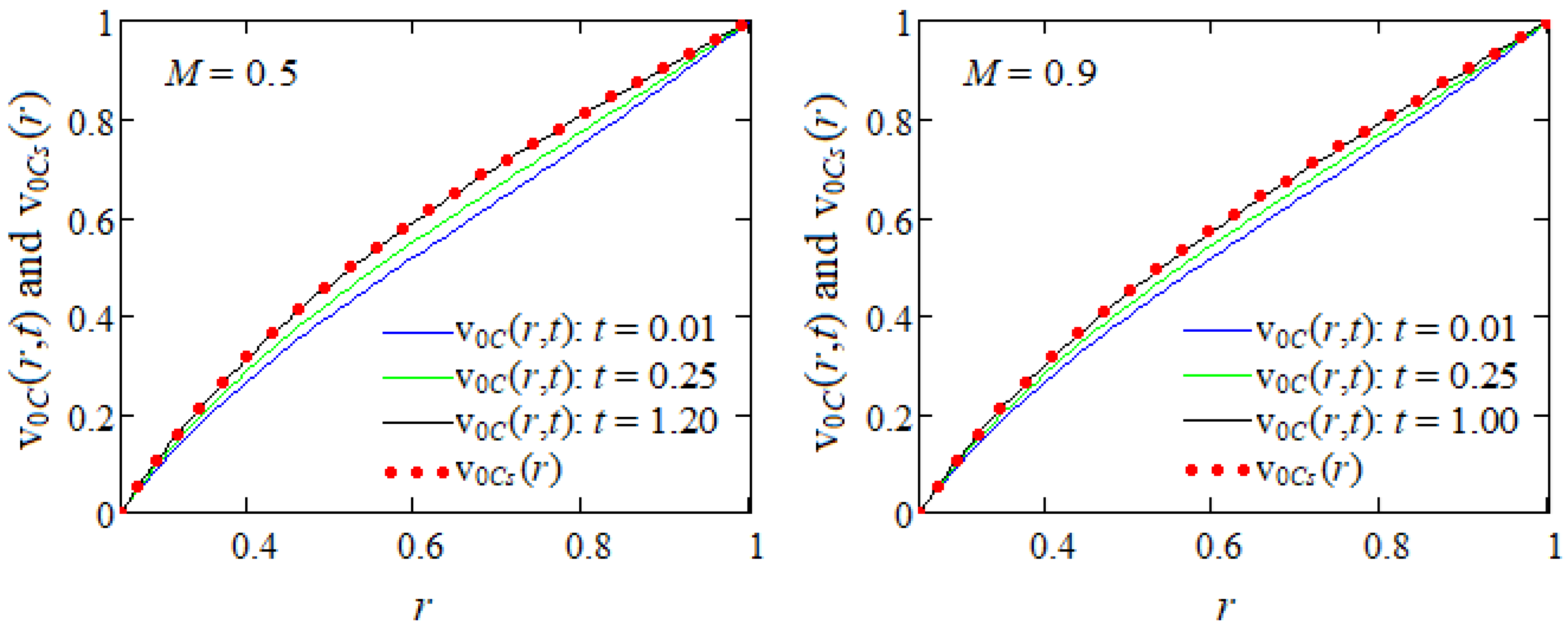
5. Numerical Results

General analytic expressions for the dimensionless velocity fields corresponding to MHD axial Couette flows of ECISGFs through a porous medium in an infinite circular cylinder and between two infinite coaxial circular cylinders have been established. Such flows describe a fairly complex fluid dynamics involving several physical phenomena. Models shearing flow situations which are useful in applications like lubrication, polymer processing and geophysical flows. For validation of the obtained results, some particular flows with technical relevance have been considered. The corresponding motions become steady in time and the starting velocity fields have been presented as sum of their steady state and transient components. The steady state components of these velocities have been presented in different forms whose equivalence was graphically proved in Figure 1 and Figure 2. Interesting expressions for the steady velocity fields corresponding to a large class of flows of these fluids have been also provided. In all cases similar solutions for electrical conducting incompressible Newtonian fluids performing the same flows can be immediately determined.

Now, in order to bring to light some characteristics of the fluid behavior and to determine the dimensionless time that is necessary to get the steady state for both types of unsteady motions, Figure 4, Figure 5, Figure 6 and Figure 7 have been prepared for increasing values of the time t, different values of the parameters K and M and fixed values for $\omega$ and $\alpha$. This time is very important for the experimental researchers who want to know the moment of transition of the motion to the steady state. It is the time after which the profile of starting velocity superposes over that of its steady component. In all cases the boundary conditions are clearly satisfied and the necessary time to reach the steady state diminishes for increasing values of the parameters K or M. In addition, as it clearly results from these figures and

Table 1. Comparative values of the steady velocity $v_{0Cs}(r)$ and starting velocity $v_{0C}(r,t)$ at dimensionless times 1.6, 1.3 and 1.2, 1 from Figure 6 and Figure 7, respectively.

r	Figure 6				Figure 7
	${\mathit{v}}_{\mathbf{0}\mathit{C}}$	${\mathit{v}}_{\mathbf{0}\mathit{C}\mathit{s}}$	${\mathit{v}}_{\mathbf{0}\mathit{C}}$	${\mathit{v}}_{\mathbf{0}\mathit{C}\mathit{s}}$	${\mathit{v}}_{\mathbf{0}\mathit{C}}$	${\mathit{v}}_{\mathbf{0}\mathit{C}\mathit{s}}$	${\mathit{v}}_{\mathbf{0}\mathit{C}}$	${\mathit{v}}_{\mathbf{0}\mathit{C}\mathit{s}}$
	$\mathit{t}=1.6$		$\mathit{t}=1.3$		$\mathit{t}=1.2$		$\mathit{t}=1$
$r_0=0.25$	0	0	0	0	0	0	0	0
0.30	0.118	0.119	0.111	0.112	0.121	0.122	0.116	0.117
0.35	0.218	0.219	0.206	0.208	0.223	0.225	0.214	0.217
0.40	0.306	0.307	0.289	0.291	0.312	0.315	0.300	0.304
0.45	0.384	0.385	0.363	0.366	0.391	0.395	0.377	0.382
0.50	0.454	0.456	0.431	0.434	0.462	0.467	0.447	0.452
0.55	0.520	0.521	0.495	0.498	0.528	0.534	0.511	0.517
0.60	0.580	0.582	0.555	0.558	0.590	0.595	0.572	0.578
0.65	0.638	0.640	0.612	0.615	0.647	0.653	0.629	0.636
0.70	0.693	0.695	0.668	0.671	0.702	0.707	0.685	0.691
0.75	0.747	0.748	0.723	0.726	0.755	0.760	0.739	0.744
0.80	0.798	0.800	0.778	0.780	0.806	0.810	0.791	0.796
0.85	0.849	0.850	0.832	0.834	0.856	0.859	0.844	0.848
0.90	0.900	0.900	0.887	0.889	0.904	0.907	0.896	0.898
0.95	0.950	0.900	0.943	0.944	0.952	0.954	0.948	0.949
1.00	1.000	1.000	1.000	1.000	1.000	1.000	1.000	1.000

, the fluid velocity grows up in time but is a decreasing function with regard to the porous and magnetic parameters K and M. Consequently, as expected, the fluid flows slower and the steady state is rather obtained under the influence of a porous medium or magnetic field. Furthermore, it also results from these figures that the steady state is earlier touched in the case of motion between infinite coaxial circular cylinders than in an infinite circular cylinder in the same conditions. This is due to the stationary inner cylinder that slows down the fluid motion.

In conclusion, when such fluids move in a magnetic field electromagnetic forces arise, affecting the flow and models shearing flow situations which are useful in applications like lubrication, polymer processing, and geophysical flows. Even though it sounds highly theoretical, the present study can be useful to models real systems in engineering, geophysics, biomedical, metalurgical processes, polymer and chemical processes, lubrication systems and environmental engineering.

6. Conclusions

Axial Couette flows of ECISGFs through a porous medium in two cylindrical domains have been analytically and numerically investigated in the presence of a magnetic field. The fluid motion is produced by an infinite circular cylinder that slides along its symmetry axis with the time-dependent velocity $Vf(t)$. General analytic expressions were established for the dimensionless velocity field $v(r,t)$ using the finite Hankel transform only. These expressions can be used to derive the fluid velocity for any motion of this kind of the respective fluids and the problems in discussion are completely solved. For illustration, some flows with engineering applications have been considered and the corresponding velocity fields have been used to bring to light some characteristics of the fluid behavior.

The main findings that have been obtained by means of this study are:

-

MHD axial Couette flows of ECISGFs through a porous medium in two cylindrical domains were analytically investigated. The fluid motion was induced by a circular cylinder that moves along its symmetry axis with the time-dependent velocity $Vf(t)$.

-

General expressions have been established for the corresponding dimensionless velocity fields. They can generate exact solutions for any motion of this type of the respective fluids and the motion problems in discussion are completely solved.

-

For illustration, some particular cases have been considered and the corresponding velocity fields were derived. For validation, the steady components of these velocities were presented in different forms and their equivalence was graphically proved.

-

As application, since the considered motions become steady in time, the necessary time to reach the steady state was graphically determined. That time, which is important for experimental researchers, declines for increasing values of K or M.

-

Consequently, the steady state for such motions of ECISGFs is earlier touched in the presence of a porous medium or magnetic field. It is also rather touched for flows between infinite circular cylinders than in an infinite circular cylinder.

-

The fluid flows faster in the absence of a porous medium or magnetic field.

In completion, we provide an important equation for the non-trivial shear stress that can be useful for readers to solve similar motion problems in which the shear stress is prescribed on the boundary. In such cases they can use the fact that the dimensionless shear stress $\tau (r,t)$ satisfies the governing equation

$$\begin{array}{l}{\displaystyle \frac{\partial \tau (r,t)}{\partial t}}=\left(1+\alpha {\displaystyle \frac{\partial }{\partial t}}\right)\left[{\displaystyle \frac{{\partial }^2\tau (r,t)}{\partial r^2}}+{\displaystyle \frac{1}{r}}{\displaystyle \frac{\partial \tau (r,t)}{\partial r}}-{\displaystyle \frac{1}{r^2}}\tau (r,t)\right]\\ -M\tau (r,t)-K\left(1+\alpha {\displaystyle \frac{\partial }{\partial t}}\right)\tau (r,t),\end{array}$$

(52)

that can be easily solved using the Hankel transforms. As soon as the shear stress $\tau (r,t)$ is determined for a given motion, the corresponding velocity field can be easily obtained solving the linear differential Equation (8).

References

1. Ting, T.W. Certain unsteady flows of second grade fluids. Arch. Ration. Mech. Anal. 1963, 14, 1–26. [Google Scholar] [CrossRef]
2. Rajagopal, K.R. Longitudinal and torsional oscillations of a rod in a non-Newtonian fluid. Acta Mech. 1983, 49, 281–285. [Google Scholar] [CrossRef]
3. Bandelli, R.; Rajagopal, K.R. Start-up flows of second grade fluids in domains with one finite dimension. Int. J. Non-Linear Mech. 1995, 30, 817–839. [Google Scholar] [CrossRef]
4. Fetecau, C. Starting solutions for the motion of a second grade fluid due to longitudinal and torsional oscillations of a circular cylinder. Int. J. Eng. Sci. 2006, 44, 788–795. [Google Scholar] [CrossRef]
5. Erdogan, M.E.; Imrak, C.E. On the comparison of the methods used for the solutions of the governing equation for unsteady unidirectional flows of second grade fluids. Int. J. Eng. Sci. 2007, 45, 786–796. [Google Scholar] [CrossRef]
6. Bano, Z.; Shah, N.F.; Islam, S.; Haroon, T. Exact solution to longitudinal and torsional oscillations of an electrically conducting second grade fluid. Int. J. Phys. Sci. 2011, 6, 2939–2943. [Google Scholar] [CrossRef]
7. Fetecau, C.; Mocanu, C.; Samiulhaq; Fetecau, C. Exact solutions for motions of second grade fluids induced by an infinite cylinder that applies arbitrary shear stresses to fluid. J. Comput. Theor. Nanosci. 2012, 17, 266–270. [Google Scholar] [CrossRef]
8. Javaid, M.; Imran, M.A.; Khan, I.; Nisar, K.S. Natural convection flow of a second grade fluid in an infinite vertical cylinder. Sci. Rep. 2020, 10, 8327. [Google Scholar] [CrossRef] [PubMed]
9. Erdogan, M.E. On unsteady motions of a second-order fluid over a plane wall. Int. J. Non-Linear Mech. 2003, 38, 1045–1051. [Google Scholar] [CrossRef]
10. Erdogan, M.E.; Imrak, C.E. Effects of the side walls on unsteady flow of a second grade fluid over a plane wall. Int. J. Non-Linear Mech. 2008, 43, 779–782. [Google Scholar] [CrossRef]
11. Yao, Y.; Liu, Y. Some unsteady flows of a second grade fluid over a plane wall. Nonlinear Anal. Real World Appl. 2010, 11, 4442–4450. [Google Scholar] [CrossRef]
12. Sultan, Q.; Nazar, M.; Ahmad, I.; Ali, U. Flow of second-grade fluid between two walls induced by rectified sine pulses shear stress. J. Mech. 2015, 31, 573–582. [Google Scholar] [CrossRef]
13. Imran, M.; Tahir, M.; Nazar, M.; Kamran, M. Some Couette flows of a second-grade fluid due to tangential stresses. Sci. Int. 2015, 27, 829–834. [Google Scholar]
14. Baranovskii, E.S.; Artemov, M.A. Steady flows of second grade fluids subject to stick-slip boundary conditions. In Proceedings of the 23rd International Conference Engineering Mechanics, Svratka, Czech Republic, 15–18 May 2017; pp. 110–113. [Google Scholar]
15. VeeraKrishna, M.; Reddy, G.S. Unsteady MHD reactive flow of second grade fluid through porous medium in a rotating parallel plate channel. J. Anal. 2018, 27, 103–120. [Google Scholar] [CrossRef]
16. Fetecau, C.; Vieru, D. General solutions for some MHD motions of second-grade fluids between parallel plates embedded in a porous medium. Symmetry 2023, 15, 183. [Google Scholar] [CrossRef]
17. Baranovskii, E.S. Analytical solutions to the unsteady Poiseuille flow of a second grade fluid with slip boundary conditions. Polymers 2024, 16, 179. [Google Scholar] [CrossRef] [PubMed]
18. Kanuri, J.V.; Chandra Sekhar, K.V.; Brahmanandam, P.S.; Ramanaiah, J.V. Analytical solutions of Poiseuille flow of second-grade fluid. J. Nav. Archit. Mar. Eng. 2024, 21, 67–77. [Google Scholar] [CrossRef]
19. Jamil, M.; Zafarullah, M. MHD flows of second grade fluid through the moving porous cylindrical domain. Eur. J. Pure Appl. Math. 2019, 12, 1149–1175. [Google Scholar] [CrossRef]
20. Fetecau, C.; Akhtar, S.; Forna, N.C.; Moroşanu, C. General solutions for MHD motions of second grade fluids through a circular cylinder filled with porous medium. Symmetry 2025, 17, 319. [Google Scholar] [CrossRef]
21. Hamza, S.E.E. MHD flow of an Oldroyd-B fluid through porous medium in a circular channel under the effect of time dependent pressure gradient. Am. J. Fluid Dyn. 2017, 7, 1–11. [Google Scholar] [CrossRef]
22. Sneddon, I.N. Fourier Transforms; McGRAW-Hill: New-York, NY, USA, 1951. [Google Scholar]
23. Debnath, L.; Bhatta, D. Integral Transforms and Their Applications, 2nd ed.; Chapman & Hall/CRC: Boca Raton, FL, USA, 2007. [Google Scholar]
Figure 1. Equivalence of the expressions of v c s ( r , t ) and v s s ( r , t ) given by the relations (17), (22) and (19), (23), respectively, for α = 0.3 , ω = π / 3 , M = 1 , K = 0.7 .
Symmetry 17 00706 g001
Figure 2. Equivalence of the expressions of v 0 c s ( r , t ) and v 0 s s ( r , t ) given by the relations (40), (44) and (42), (45), respectively, for α = 0.3 , ω = π / 3 , M = 1 , K = 0.7 and r 0 = 0.25 .
Symmetry 17 00706 g002
Figure 3. Convergence of the dimensionless starting velocities v 0 c t ( r , t ) and v 0 s t ( r , t ) to the corresponding staring velocities v c t ( r , t ) and v s t ( r , t ) , respectively, of the motion in a circular cylinder when α = 0.4 , ω = π / 3 , M = 0.8 , K = 0.6 and r 0 0 .
Symmetry 17 00706 g003
Figure 4. Convergence of the starting velocity v C ( r , t ) to its steady component v C s ( r ) given by Equation (26) for α = 0.4 , M = 0.8 , K = 0.3 and K = 0.9 and increasing values of t.
Symmetry 17 00706 g004
Figure 5. Convergence of the starting velocity v C ( r , t ) to its steady component v C s ( r ) given by Equation (26) for α = 0.4 , K = 0.3 , M = 0.5 and M = 0.9 and increasing values of t.
Symmetry 17 00706 g005
Figure 6. Convergence of starting velocity v 0 C ( r , t ) to its steady component v 0 C s ( r ) given by Equation (44) for α = 0.4 , M = 0.8 , K = 0.3 and K = 0.9 and increasing values of t.
Symmetry 17 00706 g006
Figure 7. Convergence of starting velocity v 0 C ( r , t ) to its steady component v 0 C s ( r ) given by Equation (48) for α = 0.4 , K = 0.3 , M = 0.5 and M = 0.9 and increasing values of t.
Symmetry 17 00706 g007