Dynamic Evolution Method and Symmetric Consistency Analysis for Big Data-Oriented Software Architecture Based on Extended Bigraph

Abstract

With the development of artificial intelligence technology, there are increasingly high requirements for processing big data systems. Big data systems have undergone rapid evolution in response to changing demands. Due to the complex structural connections and dispersed component positions of big data processing systems, traditional formal methods find it difficult to dynamically model their structure and position simultaneously. To address this issue, this study proposes a formal modeling framework that extends Bigraph to support the dynamic evolution of big data software architecture. This model is capable of verifying the symmetry consistency of structural connections and component positions in evolutionary systems and evaluating them through real-life case studies of banking big data systems. The results confirmed its correctness and practical feasibility.

1. Introduction

With the exponential growth of data scale and processing complexity, traditional big data architectures are undergoing a paradigm shift from rigid designs to flexible evolution. This evolution is manifested not only in the iterative updates of the technological stack but also in a fundamental enhancement of the dynamic adaptability of the entire software architecture [1,2]. From the early Hadoop batch-processing frameworks to today’s cloud-native real-time computing systems, software systems are developing an endogenous evolutionary mechanism: achieving hot-swappable component replacement through modular design, supporting incremental functional evolution via microservices architecture, and ensuring dynamic deployment environment adaptation through containerization technologies [3]. This modular evolutionary capability enables modern big data systems to maintain business continuity while achieving seamless architectural upgrades and functional expansions. The evolution and scaling of big data software architectures are, in essence, systemic responses to continuously changing computational environments and business demands.

In recent years, the rapid advancement of artificial intelligence technologies has intensified challenges such as real-time computing demands for intelligent big data applications, hybrid load balancing, and intelligent operations management [4,5]. Consequently, constructing software architectures with dynamic and location-aware characteristics has become increasingly critical. As illustrated in Figure 1, a banking big data service system consists of a Banking Service Center (BSC) and six Banking Data Centers (BDCs). Typically, each BDC comprises multiple datasets stored across multiple databases. As enhanced data sharing and circulation expand business functionalities, an increasing number of datasets will be integrated into the system. The system must not only perceive the real-time locations of computing nodes to optimize data distribution and task scheduling but also track the dynamic flow of data transmission and reception to facilitate rational load balancing adjustments. Furthermore, privacy compliance and cross-domain data governance introduce additional complexity, requiring the system to dynamically adjust data processing logic and the number of servers in relevant locations based on data distribution and access permissions to achieve both global consistency and local autonomy. Evidently, as location-dependent data services proliferate, the corresponding data processing modules must also undergo adaptive dynamic evolution. To address such requirements, it becomes imperative to construct a model from a software architecture perspective that simultaneously represents communication flows and the positional information of component modules while supporting dynamic structural adjustments. However, as shown in Figure 2, the traditional graph model for banking big data service systems only supports unidirectional communication descriptions and lacks the capability to depict component locations. To resolve these issues, we propose a dynamic evolution method for big data software architectures based on an extended Bigraph model, which incorporates bidirectional port descriptions and explicit representations of component location boundaries. This method not only fulfills the requirements for dynamic evolution modeling but also enables consistency verification during the evolution process.

The main contributions are as follows: (1) Based on the traditional Bigraph model, we extend a Bigraph model that can describe dual receiving and transmitting ports. Such a two-way communication port is conducive to the description of the real system data flow. (2) We propose a modeling method for dynamic evolution rules and big data-oriented software architecture evolution based on extended Bigraph. The extended Bigraph model can realize the dynamic change of software architecture driven by evolution rules. (3) We design a set of symmetric consistency checking algorithms for the connection structure, component location, and global evolutionary systems.

The rest of this paper is organized as follows: Section 2 reviews the related work. Section 3 introduces the notion of Bigraph and extends Bigraph. Section 4 shows a modeling method for big data-oriented software architecture based on extended Bigraph. Section 5 designs dynamic evolution rules and the evolution reaction system of BDOSA. Section 6 discusses and analyzes the evolution consistency of software architecture. In Section 7, a case studies are carried out. Section 8 makes the conclusion and the future work.

2. Related Work

2.1. Evolution Rule Design and Formal Description

In terms of designing and describing evolution rules, different sets of evolution rules are devised and outlined for various software architectures. For instance, in the context of procedure-oriented software architecture, Chen et al. [6] designed rules for adding, deleting, and replacing elements such as variables, types, and functions and implemented the application of these evolution rules on the POLUS system. Chouikh et al. [7] employed UML to formalize the corresponding rules of software evolution metamodels, conducted a comparative analysis of the distinctions between metamodels and evolution metamodels, and demonstrated the efficacy of this approach through a concrete case study. Zhang et al. [8] proposed an extended Architecture Description Language (ADL) to formally characterize the elements, parameters, and their interrelationships in performance modeling of service-oriented software architectures, which facilitates the specification of corresponding service performance evolution rules. As for Web service-oriented software architecture, Huang et al. [9] leveraged Petri nets to describe the addition, deletion, and selection rules for service components, and provided an analysis of consistency assurance after applying these rules. In the aspect of characterizing and utilizing complex network software evolution rules, Zeng et al. [10] described intricate service evolution rules such as sequential addition, concurrent addition, selective addition, sequential-concurrent reset, and sequential-selective reset during the dynamic evolution of service-oriented composition network software using Workflow Nets (WF-nets). In the context of component-oriented network software architecture evolution, Xu et al. [11] employed hypergraphs to depict complex component/connector evolution rules, including sequential replacement, parallel addition, and split-recombination. In the evolution of internetware software architecture, Zhao et al. [12] focused on utilizing algebraic methods to describe the intricate evolution rules of connectors involving triggering, utilization, collaboration, parallelism, repetition, selection, and so forth. Despite the existence of numerous methods for describing evolution rules, these methods are only capable of describing single-port, unidirectional communication relationships, falling short of meeting the requirements for describing two-port, bidirectional communication in big data systems.

2.2. Formal Modeling Methods for Software Architecture Evolution

In terms of modeling methods for software architecture evolution, software researchers initially focused primarily on UML (Unified Modeling Language). For instance, George et al. [13] described a service-based software architecture model using UML and analyzed the reconfiguration evolution process of software services through this structural model. Although UML boasts features such as a user-friendly graphical interface, strong intuitiveness, and ease of understanding, it lacks formal semantics, making it challenging to achieve a more precise and unambiguous description of software architecture evolution. ADL (Architecture Description Language) is a specialized language designed to describe software architectures. It possesses the advantage of formal semantics. In recent years, various types of ADL languages and their extensions have been developed, including B, Wright, xADL, and ACME, among others. These languages have also been employed to describe and analyze software architecture evolution. For example, Mokni et al. [14] used B language to characterize specifications, deployments, and integration information of reusable software architectures, then established a transformation mapping from B language to Dedal formalization to verify the consistency of software architectures. Taoufik et al. [15] leveraged Wright language to depict software architecture configurations, focusing on components, connectors, roles, adhesion protocols, and instances. Oquendo et al. [16] extended ADL into SosADL, which is oriented towards systems of systems, using SosADL to describe the dynamic software architecture evolution behavior of systems of systems.

In addition to the conventional UML and ADL modeling methods, many researchers in recent years have paid closer attention to the depiction and analysis of software architecture evolution using various formal methods with rigorous mathematical semantics. These primarily encompass linear algebra, process algebra, Petri nets, graphs, and other formal approaches. For instance, Rufiange et al. [17] proposed a visualization technology based on the interactive matrix to model software structure evolution in order to solve the complexity of software evolution visualization. He et al. [18] used process algebra Pi calculus to model SaaS-oriented network software architecture and extended Pi calculus operators to depict five incremental dynamic evolution rules. Song et al. [19] used the Petri nets workflow method to model the data-aware oriented service evolution process and gave a method to check the effectiveness of service evolution migration. Xu et al. [20] represented network software architecture as hypergraphs and defined evolution rules using hypergraph transformation rules, ultimately describing the dynamic evolution process of network software architecture through hypergraph grammars. Furthermore, some scholars have explored modeling network software architecture using Bigraph, a more complex formal semantics. For example, Wang et al. [21] utilized Bigraph to model aspect-oriented network software architecture evolution. Lu et al. [22] used Bigraph to model the evolution process of software architecture in a mobile environment and gave a software evolution analysis method based on Bigraph. Wachholder et al. [23] employed hierarchical Bigraph to model system-of-systems architecture, designing evolution rules for small systems joining larger systems and describing the system-of-systems’ ability to evolve in size, among other capabilities. In recent years, regarding software architectures for big data, Li et al. [24] employed graphs to model software architectures, then designed a graph grammar named Breeze to describe the evolution process of software architectures, and finally mapped this process onto a GSPN model for verification of evolution using tools. Nevertheless, this work also overlooked the description of component location information, failing to fully capture real-world scenarios for location-sensitive big data system evolution. Addressing these issues, this paper extends traditional Bigraph with bidirectional ports and proposes a dynamic evolution method for big data-oriented software architectures based on the extended Bigraph.

UML, ADL, linear algebra, process algebra, Petri nets, graphs, hypergraphs, etc., all have good semi-formal and formal semantic modeling capabilities, but there are three shortcomings: (1) bidirectional communication is difficult to characterize. ADL, linear algebra, and process algebra have been designed with corresponding communication operators to support one-way communication, but cannot simultaneously characterize two-way communication. Visualization methods such as Petri nets, graphs, and hypergraphs only use edges to support one-way communication, and require the addition of edge properties to support two-way communication descriptions. However, the descriptions of these properties are implicit and cannot be visualized. (2) Difficulty in modeling the position of components. ADL, linear algebra, and process algebra are almost powerless in modeling component positions; Formal methods such as UML, Petri nets, diagrams, and hypergraphs only support modeling the logical relationships and positions of components but cannot complete the modeling of the physical spatial positions of components. (3) The lack of dynamic semantic changes while connecting structures and component positions. UML, ADL, linear algebra, process algebra, Petri nets, graphs, hypergraphs, and others only support dynamic semantic modeling in one dimension, making it difficult to model dynamic semantics in two dimensions. In order to overcome the above difficulties, we extend the hyperedges of Bigraph’s link graph with dual tentacles, which can support bidirectional communication, and use Bigraph’s place graph to depict the nested, parallel, and other positional semantics of components. This simultaneously achieves the use of a link graph to depict connection structures and a place graph to depict the dynamic semantic changes of component positions.

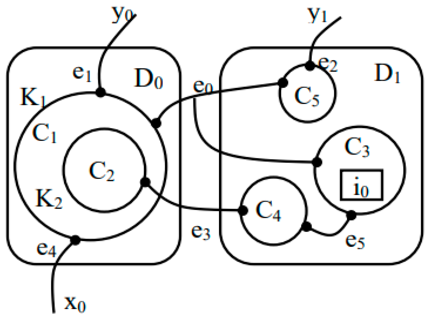
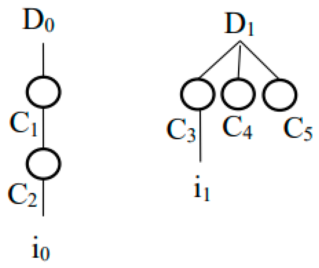
3. The Notion of Bigraph and Extended Bigraph

3.1. Static Structure and Dynamic Behavior with Bigraph

Bigraph is a graphical formal theoretical method [25], which was proposed by Robin Milner, a Turing Award winner in 2001. Bigraph has two goals: (1) modeling for pervasive computing systems; (2) building unified meta models for existing mobile and concurrent theories. A Bigraph is composed of a place graph (B^P) and a link graph (B^L), denoted as B = (B^P,B^L). Bigraph is based on the mathematical theory of s-category. In bigraph, the interface is regarded as an object and the graph is regarded as a morphism. Figure 3 is an instance of bigraph, denoted as B: <1,X>→<2,Y>, where → represents a morphism. <2,X> represents an inner interface, in which 1 denotes this bigraph has one site, that is, i₀; X denotes bigraph B has an inner name set {x₀}. <2,Y> represents an outer interface, where 2 denotes that this bigraph has two domains, that is, D₀ and D₁; Y denotes that bigraph B has an outer name set {y₀,y₁}. B^P is the place graph of bigraph B, as shown in Figure 4, denoted as B^P:1→2. B^L is the link graph of bigraph B as shown in Figure 5, denoted as B^L: X→Y. In order to enhance the ability of expression, the concept of basic signature is added into bigraph. Basic signature is characterized by a dual tuple (K, mp), where K is the control set,$\forall k\in K,k=n(n\in N)$, and n is the arity of k and N is the set of natural numbers. Any k, $k\in K$ has a map, denoted as $mp:K\to N$, which means the mapping of K to N. In other words, basic signature of bigraph is that each node is assigned a control k, and the arity n of control k is the port number of each node and n is usually represented by little black dots as depicted in Figure 1. Thus, the bigraph can be further denoted as B = (B^P,B^L) = (V,E,Ctrl,Prnt,Link): <m,X>→<n,Y>, where B^P = (V,Ctrl,Prnt): m→n and B^L = (V,E,Ctrl,Link): X→Y. V represents a finite set of nodes. E represents a finite set of edges. Ctrl:V→K represents the mapping of node V to control K. Prnt: m$\uplus$v→v$\uplus$n is the parent mapping. Link: X$\uplus$O→E$\uplus$Y is the link mapping. X is the set of inner names. n is the number of outer regions. Y is the set of outer names.

Bigraph has not only a static structure but also a dynamic structure. Dynamic structure refers to the behavior of structural change. This set of structural change behavior is called Bigraph reactive system. Figure 6 shows an example of Bigraph structural change. The light part of Figure 6 represents that PC1 in the City1 will send data d₁ to the iPhone through PC2 in the Room of the City2. The right part of Figure 6 represents that the iPhone receives the data d₁ from PC1 of City1. Multiple processes similar to this structural change are called Bigraph reactive systems.

In addition, Bigraph can not only use the observable graphics to model but it can also use its algebraic form of term language to formally infer and deduce the relevant properties of the system. There are two important operations in term language: composition operation $°$ and extended product operation $⨂$. The composition operation $U°V$ is based on the premise that the companion domain of V and the domain of U are the same. The extended product operation $U⨂V$ is to juxtapose U and V from left to right. The split parallel operator || is used to juxtapose multiple domains. The parallel operator | is used to juxtapose multiple nodes in a domain. Nesting operation () is to nest from the outside to inside, that is, from the largest domain to the smallest site.${\mathrm{e}/}_{\mathrm{m},\mathrm{n}}$ denotes edge e link ports m and n. For other operations, see reference [25]. For the example in Figure 6, we can use the term language to express it as follows: e/_p1,p2.City1(PC1(d₁))||City2(Room(PC2|iPone))$⟶$e/_p1,p2.City1(PC1)||City2(Room(PC2| iPhone(d₁))).

3.2. Extend Bigraph

In order to effectively model the connector and port in the software architecture, the edge connecting two nodes in Bigraph needs to be extended. In the original Bigraph, two nodes are connected by a super edge with only two tentacles, as shown in Figure 7. We need to extend it to the super edge of four tentacles, two of which are connected to one node and the other two to another node. For example, the connection of the two nodes shown in Figure 8 is extended to the connection of the two nodes shown in Figure 8. It is worth noting that these four tentacles have directional semantics. More specifically, they are two pairs of ports with dual semantics. As shown in Figure 8, s₁ and r₁ are a pair of sending and receiving ports, s₂ and r₂ are another pair of sending and receiving ports. Similarly, Figure 9 shows the connection of three nodes.

Definition 1 

(Extend Bigraph). the extend Bigraph is defined as B = (B^P, B^L) = (V, E*, Ctrl, Prnt, Link*), where B^P = (V, Ctrl, Prnt) and B^L = (V, E*, Ctrl, Link*). V denotes a finite set of nodes. E* denotes the super edge set of n tentacles, n is even number, n $\ge$ 4, which each e $\in$ E* form n/2 pairs of sending and receiving tentacles, that is, e = {s₁, r₁, s₂, r₂, …, s_n/2, r_n/2}, and any pair tentacles (s_i, r_i) links between two nodes. Ctrl: V $\to$ K denotes the mapping of node V to control K, that is, node type. Prnt: m $\uplus$ v → v $\uplus$ n denotes the parent mapping. Link: X $\uplus$ P → E* $\uplus$ Y is the link mapping.

Definition 2 

(Reaction Rule of Extend Bigraph). The reaction rule of extend Bigraph is p = (L, R), which is also generally denoted as p: L $⟶$ R, which means that the extend sub-Bigraph L becomes the extend sub-Bigraph R.

The reaction rule is used to describe the change process of the extended Bigraph. For example, suppose that there is a extend Bigraph B, given a reaction rule of extend Bigraph p: L $⟶$ R, the change process is equivalent to finding L in B, then replacing L with R, and the remaining part after L is removed from B remains unchanged, so that B becomes $B^{\prime }$, denoted as B $\underset{p}{\to }{B}^{\prime }$.

Definition 3 

(Reaction System of Extend Bigraph). It is a 4-tuple S = (B_N, B_T, P, B₀), where B_N denotes a finite set of non-terminal Bigraphs, B_T denotes a finite set of terminal Bigraphs, P is a finite set of Bigraph reaction rules, and B₀ is the initial Bigraph. In other words, when B₀ becomes B_n through n reaction rules, denoted as $B_0\underset{p_1}{\to }{B}_1\underset{p_2}{\to }{B}_2\cdots B_{n-1}\underset{p_n}{\to }{B}_n$, this transformation process is called a extend Bigraph reaction system, where {B₁, B₂, …, B_n−1} is a finite set of non-terminal Bigraphs, {B_n} is a finite set of terminal Bigraphs, {p₁, p₂, …, p_n} are a finite set of Bigraph reaction rules, and B₀ is the initial Bigraph.

For the convenience of expression, we also extend the term language of Bigraph. We mainly extend the super edge and arrange the pairs of ports involved in a super edge, such as N₁/s₁, r₁, s₂, r₂, …, s_n, r_n. In addition, we also display the ports on the node. For instance, if node C₁ has ports s₁ and r₁, it is denoted C1._s1,r1. Others remain unchanged, and the specific meaning is shown in

Table 1. Meaning of Bigraph term language.

Notation	Meaning
$\left|\right|$	Domain split parallel operator
$|$	Node parallel operator
$°$	Node composition operator
$⨂$	Domain juxtaposition extended operator
( )	Domain or component nesting operator
/	Link operator

.

4. Modeling Big Data-Oriented Software Architecture Based on Extend Bigraph

As the whole framework of a software system, software architecture usually includes components, connectors, and constraints. No loss of generality, big data-oriented software architecture as a specific application-oriented software architecture also has these basic elements. In addition, because big data is usually used for analysis and mining, its storage and acquisition are distributed, that is, a single application requires multiple data sets in different locations. In order to enable the system to quickly discover and query capabilities, the location information of components needs to be considered in the software architecture.

Definition 4 

(Extend Bigraph Model of Big Data-Oriented Software Architecture). The big data-oriented software architecture is represented as a four tuple BDOSA = (C, N*, S, P, Ctrl, Prnt, Link*), where C denotes the set of components; N* denotes the set of connectors, each n$\in$N* form n/2 pairs of sending and receiving ports, that is, n = {s₁, r₁, s₂, r₂, …, s_n/2, r_n/2}, and any pair ports (s_i, r_i) links between two components. Ctrl: C $\to$ K denotes the mapping of component C to control K, that is, component type. S denotes the set of constraints; P denotes the set of places; Prnt: m $\uplus$ c → c $\uplus$ n denotes the parent mapping of component and place. Link: X $\uplus$ O → N* $\uplus$ Y is the link mapping between component and port. In addition, we set a constraint in position that the same type of components can only be located in the same domain or the same component.

As shown in

Table 2. The mapping relation between BDOSA and extended bigraph.

BDOSA	Extend Bigraph
Component	Node
Connector	Super edge
Port	The tentacle of super edge
Component type	Control
Constraints	Control
Place	Domain and site

, there is a good mapping between the big data-oriented software architecture and the extended Bigraph. Figure 10 shows a simple example of big data-oriented software architecture, including four components, i.e., Client, Control Server, Manager Server, and Data Server; three connectors, i.e., N₁, N₂, N₃, each connector has corresponding matching send and receive ports, for example, N₁ has s₁, r₁, s₂, r₂; three places, i.e., Client Location, Service Center, and Data Center; and one constraint S₁, it means that there can be no connector with communication port mismatch between two components.

5. The Dynamic Evolution of BDOSA

5.1. Dynamic Evolution Rules of BDOSA

Evolution rule is the basic rule to guide software evolution, which is usually divided into three types: adding evolution rule, replacing evolution rule, and deleting evolution rule. In order to make the software architecture change dynamically, we need to design these evolution rules in advance.

In the big data-oriented software architecture, for adding a component, not only the link between the added component and other components, but also the place of the added component should be considered. Therefore, we design three basic add evolution rules, as shown in Figure 11. Evolution rule p1 denotes that there is already a component C₁ in place P₁. Now it is necessary to add a component C₂ in the same place and add the corresponding link N₁ to connect the two components. For example, in a big data distributed system, there is already a data node C₁ within a certain bank P₁, and now it is necessary to add another data node C₂. Evolution rule p2 denotes that there are already places P₁ and P₂, and a component C₁ in place P₁. Now it is necessary to add a component C₂ in the place P₂ and add the corresponding link N₁ to connect the two components. For example, in a big data distributed system, one bank P₁ already has a data node C₁, and now it is necessary to add a data node C₂ in bank P₂. Evolution rule p3 denotes that there is already a component C₁ in place P₁. Now it is necessary to add a component C₂ in the component C₁ and add corresponding link N₁ to connect the two components. For example, in a big data distributed system, there is already a data node C₁ within a bank P₁, and now it is necessary to add a security protection node C₂ within the data node C₁. We also can express it with the term expression in Bigraph, as follows.

p1: P₁(C₁) $\to$ N₁$/$s₁, r₁, s₂, r₂. P₁(C_1.s1,r2$|$C_2.s2,r1);

p2: P₁(C₁)$\left|\right|$P₂ $\to$ N₁$/$s₁, r₁, s₂, r₂. P₁(C_1.s1,r2)$\left|\right|$P₂(C_2.s2,r1);

p3: P₁(C₁) $\to$ N₁$/$s₁, r₁, s₂, r₂. P₁(C_1.s1,r2 (C_2.s2,r1));

To the replace evolution rule, we also design three basic replace evolution rules, as shown in Figure 12. Evolution rule p4 denotes that there are already two components C₁ and C₂ in place P₁, and the corresponding link N₁ to connect the two components. Now it is necessary to replace component C₂ with $C_2^{\prime }$, and the other parts remain unchanged. For example, in a big data distributed system, there are two data nodes C₁ and C₂, within a bank of P₁, and now it is necessary to replace data node C₂ with $C_2^{\prime }$. Evolution rule p5 denotes that there are already two components, C₁ and C₂, in the place of P₁ and P₂, respectively, and the corresponding link N₁ to connect the two components. Now it is necessary to replace component C₂ with $C_2^{\prime }$, and the other parts remain unchanged. For example, in a big data distributed system, spanning two banks, P₁ and P₂, there is a data node C₁ within one bank, P₁, and the no data node, P₂. Now, it is necessary to add a data node C₂ within P₂. Evolution rule p6 denotes that there are already two components C₁ and C₂ in place P₁, and C₂ is in C₁, and the corresponding link N₁ to connect the two components. Now it is necessary to replace component C₂ with $C_2^{\prime }$, and the other parts remain unchanged. For example, in a big data distributed system, there is a data node C₁ in bank P₁, and there is a security protection node C₂ inside the data node C_1. Now it is necessary to replace the security protection node C₂ with $C_2^{\prime }$. We can also express it with the term expression in Bigraph, as follows.

p4: N₁$/$s₁,r₁,s₂,r₂.P₁(C_1.s1,r2$|$C_2.s2,r1)$\to$N₁$/$s₁,r₁,s₂,r₂.P₁(C_1.s1,r2$|{\mathrm{C}}_2^{\prime }$_.s2,r1);

p5: N₁$/$s₁,r₁,s₂,r₂.P₁(C_1.s1,r2)$\left|\right|$P₂(C_2.s2,r1)$\to$N₁$/$s₁,r₁,s₂,r₂.P₁(C_1.s1,r2)$\left|\right|$P₂(${\mathrm{C}}_2^{\prime }$_.s2,r1);

p6: N₁$/$s₁,r₁,s₂,r₂.P₁(C_1.s1,r2 (C_2.s2,r1))$\to$N₁$/$s₁,r₁,s₂,r₂.P₁(C_1.s1,r2 (${\mathrm{C}}_2^{\prime }$_.s2,r1));

To the delete evolution rule, we also design three basic replace evolution rules, as shown in Figure 13. Evolution rule p7 denotes that there are already two components, C₁ and C₂ in the place of P₁, and the corresponding link N₁ to connect the two components. Now it is necessary to delete component C₂ and the corresponding link N₁, and the other parts remain unchanged. For example, in a big data distributed system, there are two data nodes, C₁ and C₂, within a bank P₁, and now it is necessary to delete data node C₂. Evolution rule p8 denotes that there are already two components C₁ and C₂ in the place of P₁ and P₂, respectively, and the corresponding link N₁ to connect the two components. Now it is necessary to delete component C₂ and the corresponding link N₁, and other parts remain unchanged. For example, in a big data distributed system, there are data nodes C₁ and C₂ in the two banks, P₁ and P₂, respectively. Now it is necessary to delete data node C₂ in P₂. Evolution rule p9 denotes that there are already two components C₁ and C₂ in place P₁, and C₂ is in C₁, and the corresponding link N₁ to connect the two components. Now it is necessary to delete component C₂ and the corresponding link N₁, and the other parts remain unchanged. For example, in a big data distributed system, there is a data node C₁ within bank P₁, and there is a security protection node C₂ within the data node C₁. Now it is necessary to delete the security protection node C₂. We can also express it with the term expression in Bigraph, as follows.

p7: N₁$/$s₁,r₁,s₂,r₂.P₁(C_1.s1,r2$|$C_2.s2,r1)$\to$P₁(C₁);

p8: N₁$/$s₁,r₁,s₂,r₂.P₁(C_1.s1,r2)$\left|\right|$P₂(C_2.s2,r1)$\to$P₁(C₁)$\left|\right|$P₂;

p9: N₁$/$s₁,r₁,s₂,r₂.P₁(C_1.s1,r2 (C_2.s2,r1))$\to$P₁(C₁);

5.2. Dynamic Evolution of BDOSA Based on Evolution Rules

Software dynamic evolution is based on evolution rules. In other words, only under the driving of evolution rules, software architecture evolution can be completed.

Proposition 1 

(Availability of evolution rule). Suppose p: L$⟶$R is an evolution rule of BDOSA, and B is an extended Bigraph model of BDOSA, if L from the left part of p is a sub Bigraph of B, then the evolution rule p can be applied to the extended Bigraph model B of BDOSA.

Proof. 

Suppose p1, p2, p3, p4, p5, p6, p7, p8, p9 are one of the evolution rules. It can be seen from Figure 11, Figure 12 and Figure 13 that the left part of these rules is a small Bigraph, and BDOSA also is a Bigraph. Obviously, the left part of these rules, L, is the part to be replaced in the Bigraph. Therefore, if the left part of these rules can be found in the Bigraph, then the evolution rules are obviously available. □

Definition 5 

(Reaction system of software architecture evolution). It is a 4-tuple RS = (BDOSA_N, BDOSA_T, P, BDOSA₀), where BDOSA_N denotes a finite set of non-terminal software architectures of extend Bigraph model, BDOSA_T denotes a finite set of terminal software architectures of extend Bigraph model, P is a finite set of evolution rules, and BDOSA₀ is the initial software architecture of extend Bigraph model. In other words, when BDOSA₀ becomes BDOSA_n through n evolution rules, denoted as ${BAOSA}_0\underset{p_1}{\to }{BAOSA}_1\underset{p_2}{\to }{BAOSA}_2\cdots {BAOSA}_{n-1}\underset{p_n}{\to }{BAOSA}_n$, this transformation process is called a reaction system of software architecture evolution, where {BDOSA₁, BDOSA₂, …, BDOSA_n−1} is a finite set of non-terminal terminal software architectures of extend Bigraph model, {BDOSA_n} is a finite set of terminal terminal software architectures of extend Bigraph model, {p₁, p₂, …, p_n} are a finite set of evolution rules, and BDOSA₀ is the initial terminal software architectures of extend Bigraph model.

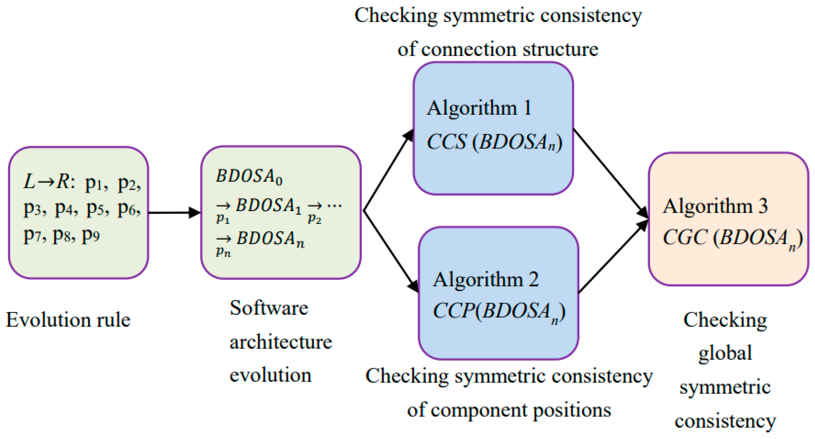
6. Symmetric Consistency Analysis of Software Architecture Evolution

Definition 6 

(Symmetric consistency of connection structure). If there is a software architecture BDOSA₁ that satisfies the constraint that connections between components are made through connectors N, and any one of the dual tentacles (s_i, r_i) of connector N can only connect to one component, then when BDOSA₁ evolves into BDOSA₂, BDOSA₂ still satisfies this constraint. Then, it is said that evolved BDOSA₂ satisfies symmetric consistency of connection structure.

Proposition 2 

(Keeping the evolutionary symmetric consistency of the connection structure). Assuming there is a software architecture BDOSA₁ that satisfies the constraint that connections between components are made through connectors N, and any one of the dual tentacles (s_i, r_i) of connector N can only connect to one component. If BDOSA₂ is evolved using any one or more of p₁–p₉ evolution rules, it can keep the symmetric consistency of its connection structure.

Proof. 

(1) In the above description, since adding evolutionary rules p₁, p₂, and p₃ during component addition will also add a connector N, and each dual tentacles (s_i, r_i) of the connector only corresponds to one component, using any number of additional evolutionary rules can evolve BDOSA₂ while keeping symmetric consistency in connection structure. (2) During the process of replacing components with evolutionary rules p₄, p₅, and p₆, only the component itself is replaced without changing the connectors or their corresponding dual tentacles (s_i, r_i). Therefore, BDOSA₂, which can evolve using any number of replacement evolutionary rules, can keep symmetric consistency in its connection structure. (3) Deleting the evolutionary rules p₇, p₈, and p₉ will also delete their connected dual tentacles (s_i, r_i) during the component deletion process without dangling tentacle, so BDOSA₂ that can evolve using any multiple times of deleting evolutionary rules can keep the symmetric connection structure symmetric consistency. Based on the (1)–(3) cases, it can be seen that after using any one or more of the evolution rules in p₁–p₉ to become BDOSA₂, the evolved BDOSA₂ must keep symmetric consistency in connection structure. □

We design Algorithm 1 to check the symmetry consistency of the connection structure. Its main idea is to traverse each node and check whether there are connectors between each node and its adjacent nodes. Then, traverse each connector and check whether the dual transmit and receive tentacles on each connector are connected to the same node. If either of these two conditions is not met, it is judged that the connection structure is symmetrically inconsistent. The specific details are as follows.

Algorithm 1: Checking Symmetric Consistency of Connection Structure, CCS

Input: Software architecture BDOSA = (C, N*, S, P, Ctrl, Prnt, Link*)

Output: Consistent_Structure of No_Consistent_Structure

$1:\mathbf{for}\forall$ci $\in$ C     // Traverse each node

$2:\mathbf{if}\mathrm{there}\mathrm{is}n\mathrm{between}{c}_i\mathrm{and}{c}_j,\mathrm{where}{c}_j\in$C$,n\in$N*

$3:C\leftarrow$ C–ci

4:   else

5:     return No_Consistent_Structure

6: end for

$7:\mathbf{for}\forall$ni $\in$ N // Traverse each connector

$8:\mathbf{if}\mathrm{any}\forall$$(s_i,r_i)\in$ ni$\mathrm{is}\mathrm{only}\mathrm{linked}\mathrm{to}\forall$ci $\in$ C

$9:N\leftarrow$ N*–ni

10:  else

11:    return No_Consistent_Structure

12: end for

13: return Consistent_Structure

Definition 7 

(Symmetric consistency of component positions). If there is a software architecture BDOSA₁ that satisfies the constraint that n types of components C₁, C₂, …, C_n can only be located in n types of positions P₁, P₂, …, P_n, respectively, and when BDOSA₁ evolves into BDOSA₂, BDOSA₂ still satisfies this constraint, then it is said that evolved BDOSA₂ satisfies component positions consistency.

Proposition 3 

(Keeping the evolutionary consistency of component positions). Assuming there is a software architecture BDOSA₁ that satisfies constraints such that n types of components C₁, C₂, …, C_n can only be located in n types of positions P₁, P₂, …, P_n, respectively, if any one or more of p₁–p₉ are used to evolve into BDOSA₂, then the evolved BDOSA₂ keeps symmetric consistency of component positions.

Proof. 

(1) Deleting evolutionary rules p₇, p₈, and p₉ during the deletion of components will not change the position of other components, so BDOSA₂ that can evolve using any number of delete evolutionary rules can maintain symmetric consistency of component positions. (2) During the process of replacing components with evolutionary rules p₄, p₅, and p₆, only the position of the replacement component is changed without altering the positions of other components. Therefore, using any number of replacement evolutionary rules to evolve BDOSA₂ can keep the symmetric consistency of component positions. (3) Adding evolution rules p₁ adds the same type of components and their parallel relationships in the same domain, while adding p₂ adds heterogeneous components that explicitly define two domains. Adding p₃ includes components that are nested within a single domain, so using any number of additional evolution rules can keep symmetric consistency of component positions for BDOSA₂ that evolves. Based on the (1)–(3) scenarios, it can be seen that after using any one or more of the evolution rules in p₁–p₉ to become BDOSA₂, the evolved BDOSA₂ will always keep symmetric consistency of component positions. □

We design Algorithm 2 to check the symmetry consistency of component positions. Its main idea is to first classify the components. Then, it is necessary to separately check whether all components in each category are in the same position. If there is any inconsistency in the position of one component, it is judged as a symmetrical inconsistency in the position of the component. The specific details are as follows.

Algorithm 2: Checking Symmetric Consistency of Component Positions, CCP

Input: Software architecture BDOSA = (C, N*, S, P, Ctrl, Prnt, Link*)

Output: Consistent_Location of No_Consistent_Location

$1:{\mathit{Ck}}_i\leftarrow \varnothing$    // Component classification variable

$2:\mathit{Ck}\leftarrow \varnothing$    // Component classification set

$3:\mathbf{for}\forall$ci $\in$ C    // Classification

$4:\mathbf{if}\mathit{Ctrl}:c_i\to$ ki

$5:{\mathit{Ck}}_i\leftarrow$  Cki $\cup$ ci

$6:\mathit{Ck}\leftarrow$ Ck $\cup$ Cki

7:   end if

8: end for

$9:\mathbf{for}\forall$Cki $\in$ Ck   // Discriminant location

$10:\mathrm{if}\forall$ci $\in$ Cki$,c_i\mathrm{is}\mathrm{located}\mathrm{in}\mathrm{the}\mathrm{same}{P}_i\in$ P

11:      return Consistent_Location

12:   else

13:      return No_Consistent_Location

14: end for

Definition 8 

(Global symmetric consistency of software architecture). If there is a software architecture BDOSA₁, when BDOSA₁ evolves into BDOSA₂, and BDOSA₂ satisfies the consistency of connection structure and component location, then it is said that evolved BDOSA₂ satisfies the consistency of component location.

Proposition 4 

(Keeping global symmetric consistency of evolving software architecture). Assuming there exists a software architecture BDOSA₁, if n evolution rules are used to transform BDOSA₁ into BDOSA_n, denoted as ${BDOSA}_0\underset{p_1}{\to }{BDOSA}_1\underset{p_2}{\to }{BDOSA}_2\cdots {BDOSA}_{n-1}\underset{p_n}{\to }{BDOSA}_n$, where p_i$\in${p₁, p₂, …, p_n}, then the evolved BDOSA_n can keep global symmetric consistency.

Proof. 

Since the evolution process is based on evolutionary rules, according to Propositions 2 and 3, it can be seen that each use of an evolutionary rule ensures symmetric consistency in the connection structure and component location of the evolved software architecture. Therefore, after n iterations of evolution, BDOSA_n keeps global symmetric consistency. □

We also designed Algorithm 3 to check global symmetry consistency in software architecture. Its main idea is that when both the symmetry consistency of the connection structure and the symmetry consistency of the component position are satisfied, it can be judged as global symmetry consistency. Otherwise, if one of the symmetry consistency is not satisfied, then the global symmetry consistency is not satisfied. The specific details are as follows.

Algorithm 3: Checking Global Symmetric Consistency of Software Architecture, CGC

Input: Software architecture BDOSAn = (C, N*, S, P, Ctrl, Prnt, Link*)

Output: Consistent_Global of No_Consistent_Global

$1:\mathit{CS}\leftarrow \varnothing$      // Temporary variable

$2:\mathit{CL}\leftarrow \varnothing$     // Temporary variable

3:  if CCS(BDOSAn) = true

$4:\mathrm{CS}\leftarrow$Consistent_Structure

5:  else

6:    return No_Consistent_Global

7:   if CCP(BDOSAn) = true

$8:\mathit{CL}\leftarrow$Consistent_Structure

9:  else

10:    return No_Consistent_Global

$11:\mathbf{if}\mathrm{CS}\bigwedge$CL$\ne \varnothing$

12:     return Consistent_Global

13:  else

14:    return No_Consistent_Global

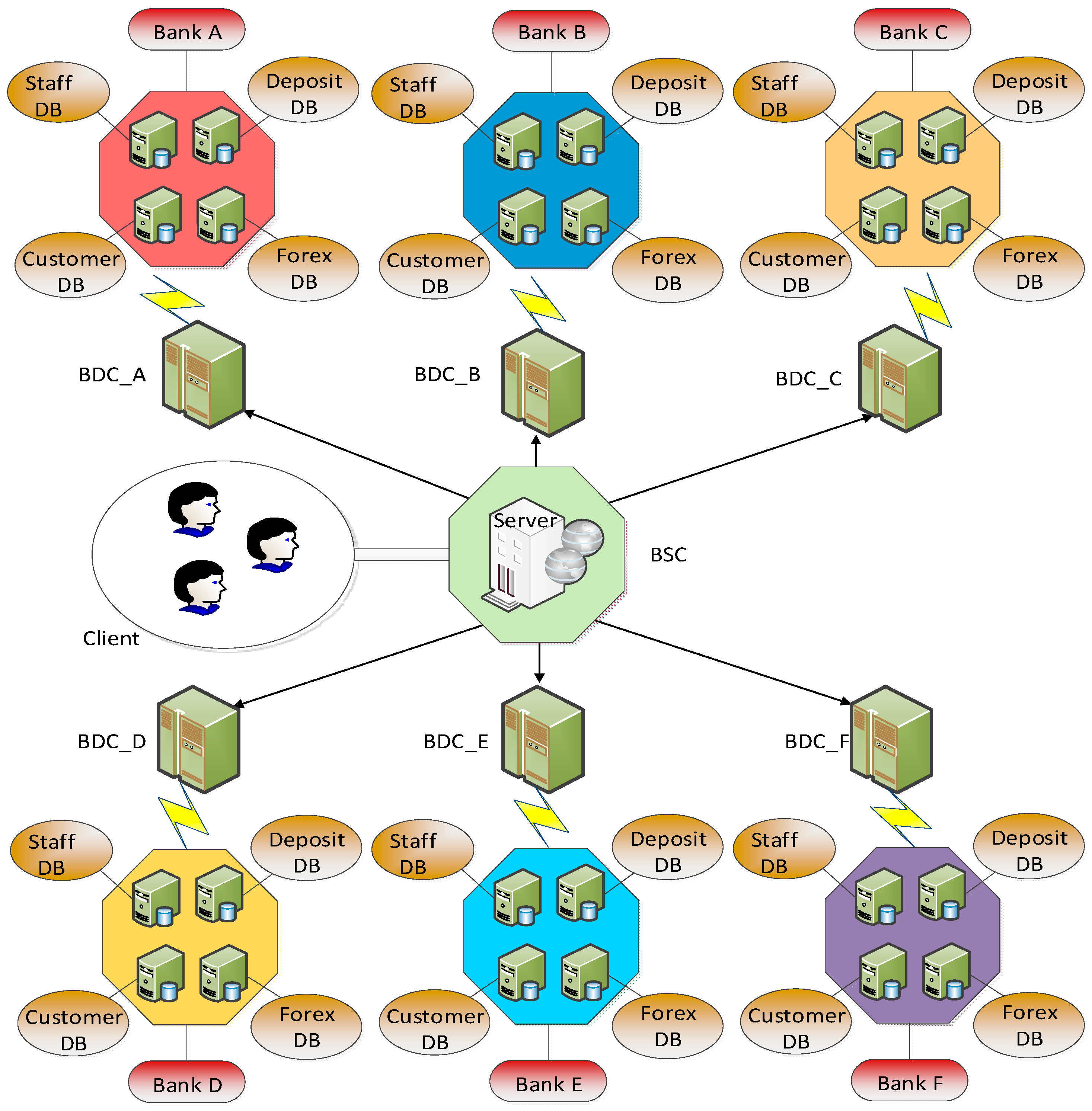
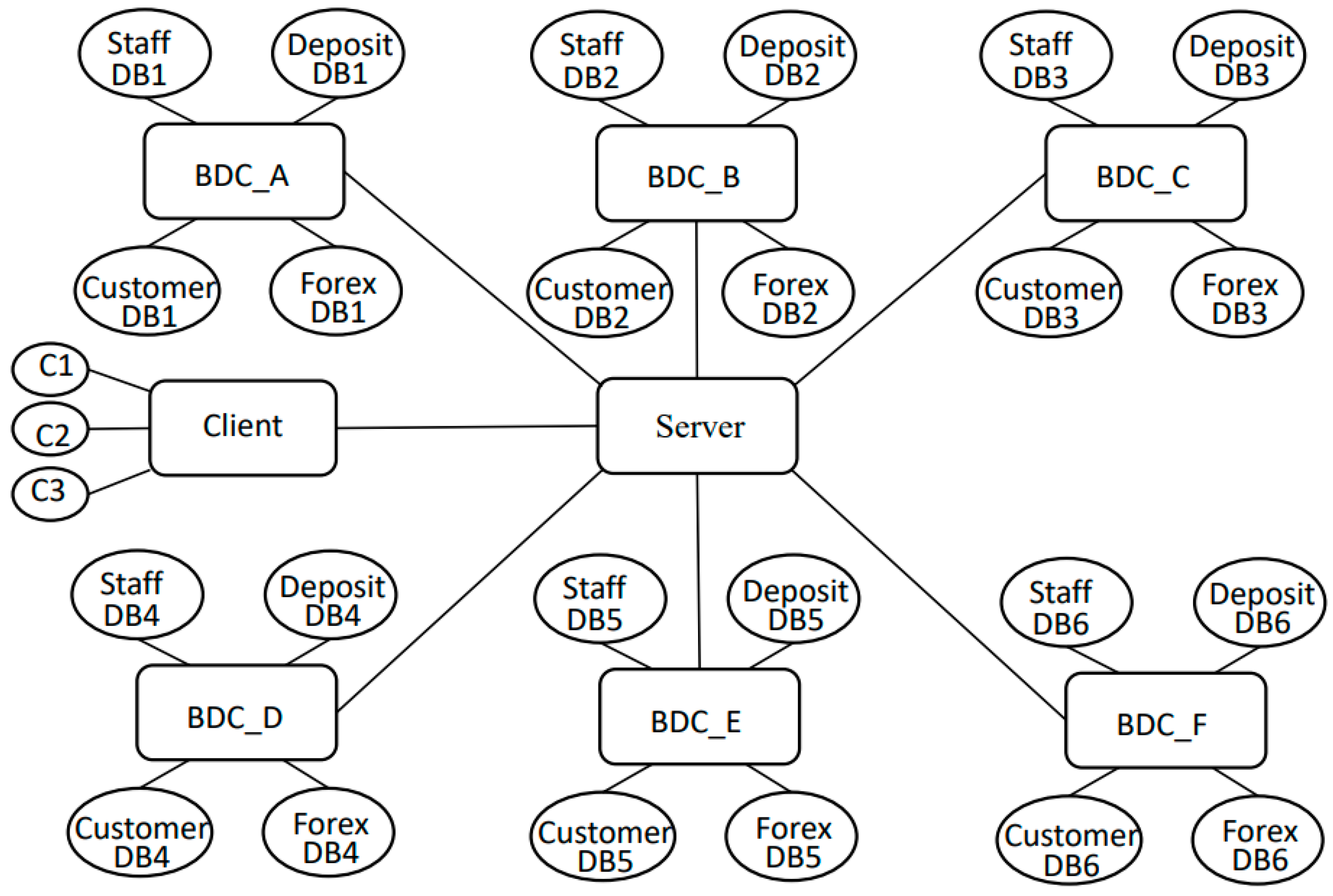
In summary, as shown in Figure 14, the consistency checking process for big data-oriented software architecture evolution is illustrated. Driven by the evolution rule L$⟶$R, the software architecture undergoes n evolutions and eventually evolves into BDOSA_n. Then, the algorithms CCS and CCP were used to check consistency in connection structure and component location for BDOSA_n. Finally, global symmetric consistency was detected using the algorithm CGC.

7. Case Studies

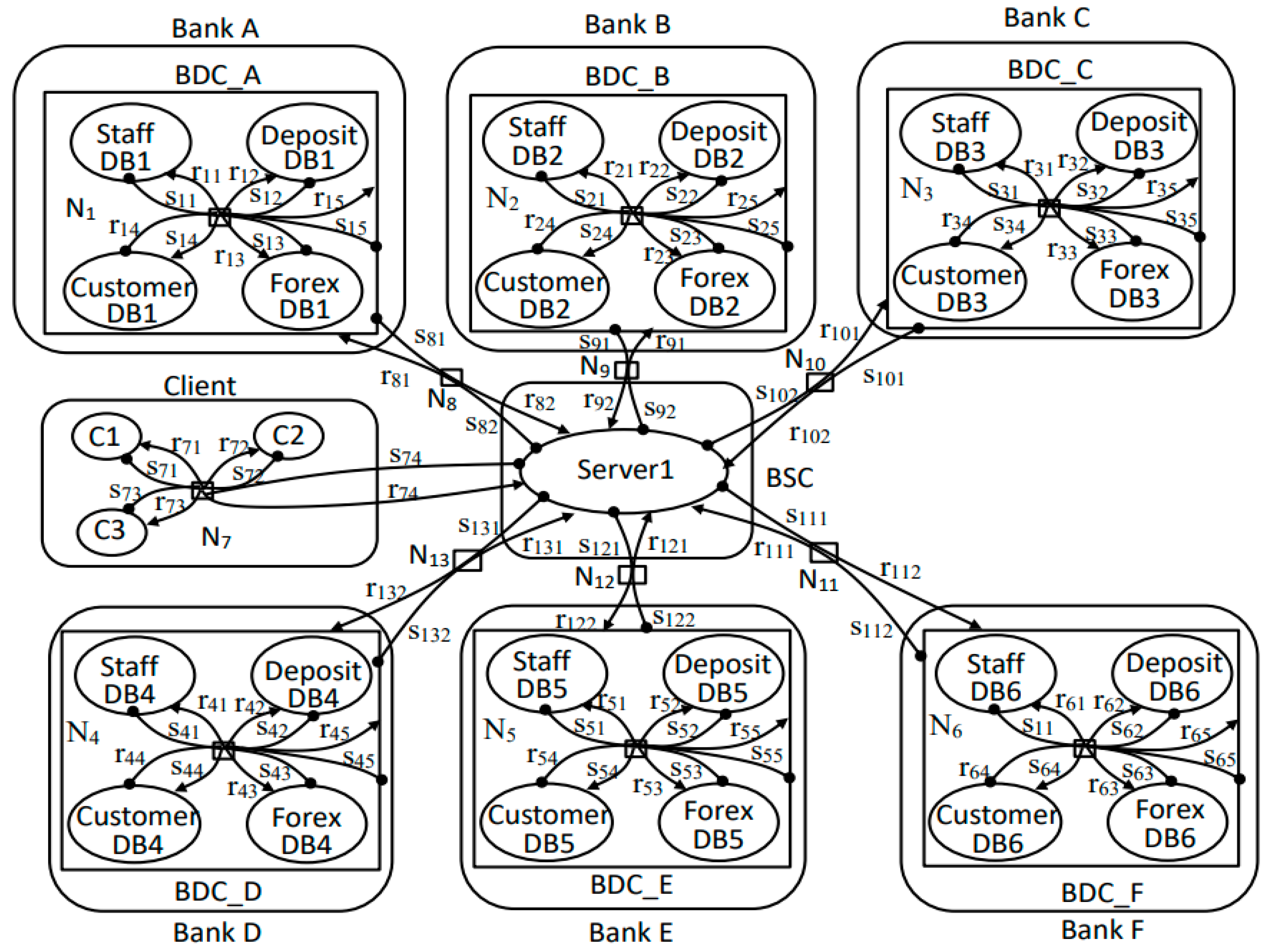
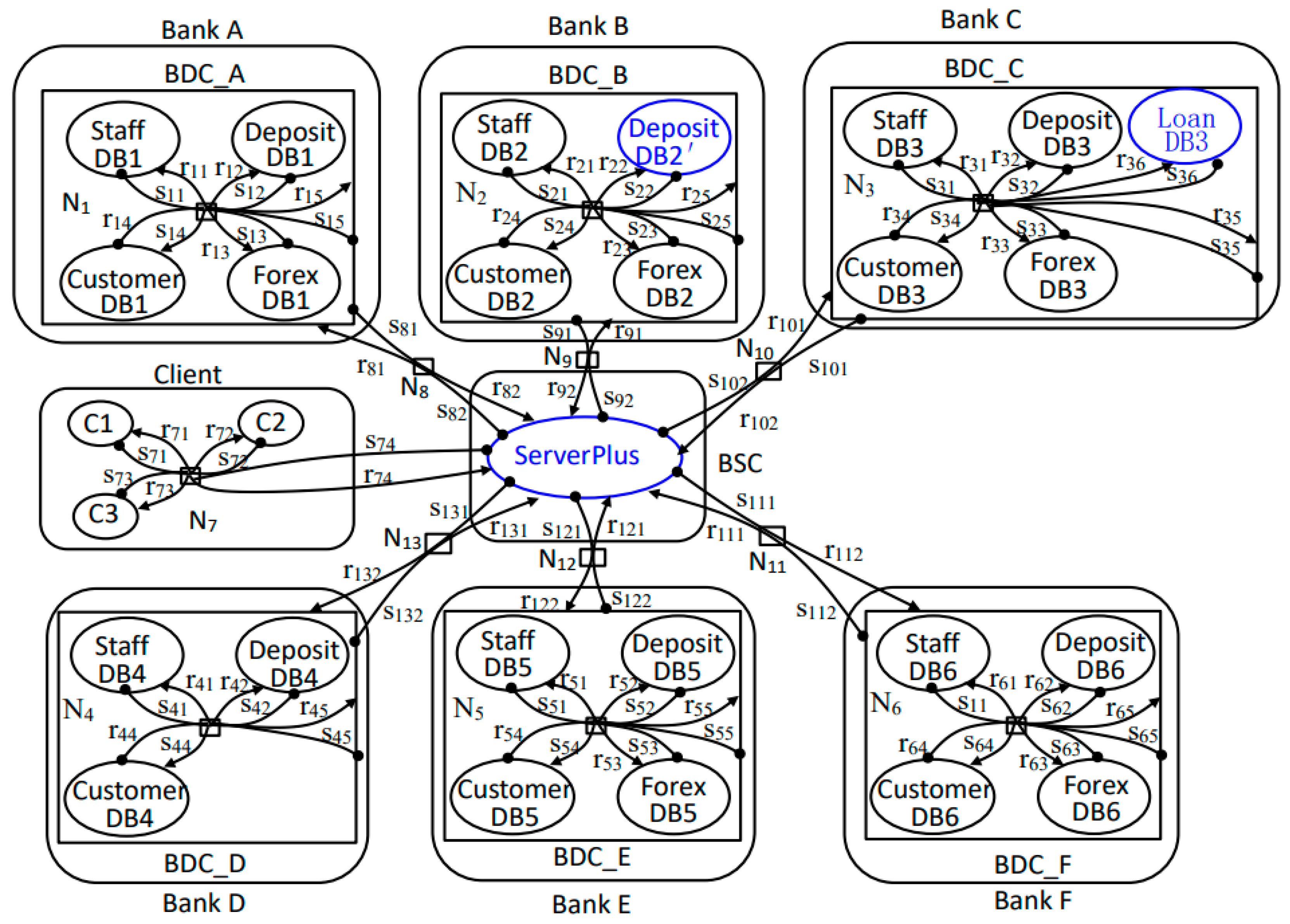
7.1. Bigraph Model of Bank Data Service System

The original structure of the bank data service system and the software architecture diagram are, respectively presented in Figure 1 and Figure 2. We are now using Extended Bigraph to model its software architecture. As shown in Figure 15, the Bigraph model of the software architecture of the bank data service system includes eight domains, namely Bank A, Bank B, Bank C, Bank D, Bank E, Bank F, BSC, and a virtual location for the Client. Each Bank i has a data center server component BDC_i deployed separately, and each data center server manages and deploys four types of database server components: Staff DBi, DepositDBi, ForexDBi, and CustomerDBi. This is represented as a nested relationship of virtual locations in the Bigraph model. A powerful control server component, Server1, is deployed in the BSC, and there are three types of clients C1, C2, and C3 in the Client. These components are connected through connectors N_i, and communication between components is performed through dual transceiver ports (s_i, r_i), which are represented as dual tentacles on Bigraph as super-edges.

Compared with the general graph modeling in Figure 2, the Bigraph model can not only clearly depict the location information consistent with the practice scenario, such as BankA, Bank B, BankC, etc., but also clearly describe the logical inclusion relationship in the actual scenario, such as BDC_A logically managing four types of database servers: Staff DB1, DepositDB2, ForexDB3, and CustomerDB4. It uses nested relationships to depict the logical inclusion relationship. In terms of connectivity, as shown in Figure 2, components can only be simply associated with each other through a single edge. In the Bigraph model, components are connected through connectors N_i, which are super-edges with dual tentacles. They can not only describe one-to-many and many-to-many relationships but also describe the communication and exchange of data between components, allowing for a more detailed depiction of the service data flow between components. For instance, when C1 requests Bank C to query its deposit, the entire flow of service data from initiating the request to receiving the response can be described as follows: C1$\to$s₇₁$\to$r₇₄$\to$Server1$\to$s₁₀₂$\to$r₁₀₁$\to$BDC_C$\to$s₃₅$\to$r₃₂$\to$DepositDB3$\to$s₃₂$\to$r₃₅$\to$BDC_C$\to$s₁₀₁$\to$r₁₀₂ $\to$Server1$\to$s₇₄$\to$r₇₁$\to$C1. It is evident that the Bigraph model can better depict the intricate connections and location information that closely resemble real-world scenarios, providing a solid foundation for subsequent evolutions.

7.2. System Evolution

In the big data service system of the bank, due to the increasing demand for various functional businesses and online financial services of the bank, the system needs to upgrade its corresponding data services. For example, due to the surge of deposit business in some banks, the bank data center needs to update the corresponding large-capacity database. In order to deal with large-scale online real-time financial business, the bank’s big data service system needs to replace the low-performance data distribution server with high-performance data distribution server. Some banking businesses are subject to policy constraints and will stop foreign exchange transaction data services for a long time. The database that stops data services needs to be uninstalled in time. However, the 24 h online demand of modern financial services cannot tolerate any service interruption, and the upgrading or maintenance of these databases and servers needs to be carried out online without downtime. The evolution rules designed in this paper take into account the connection and location of the components that need to evolve, so they are strictly formal constraints when designing rules, which can guide the system to evolve reliably. The use of these rules in the evolution of the bank’s big data service system will be shown in detail below.

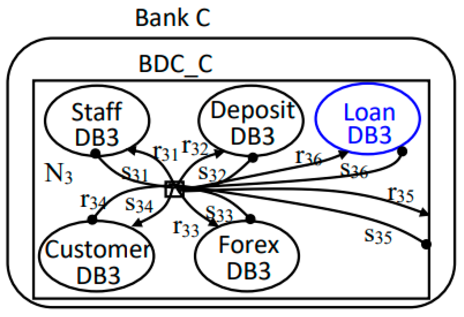
7.2.1. Add Evolution Rules

With the rapid development of online mobile technology, the demand for online loan services has surged significantly, necessitating the expansion of online loan business functions. To ensure safety, an online loan service application pilot will first be conducted at Bank C, with a view to extending it to the entire banking system once stable operations are achieved. By analyzing the logic of business functions, we have determined that a dedicated loan service database server needs to be added. Correspondingly, this requires the inclusion of a loan function component, which will exist in parallel with StaffDB3, DepositDB3, ForexDB3, and CustomerDB3 as a similar type of component. Given this scenario, we have chosen the evolution rule p1 to conduct a systematic Bigraph evolution upgrade. The corresponding section of the system’s Bigraph model after the addition of the loan function component is illustrated in Figure 16. For the sake of simplicity, only the evolutionary parts are presented here.

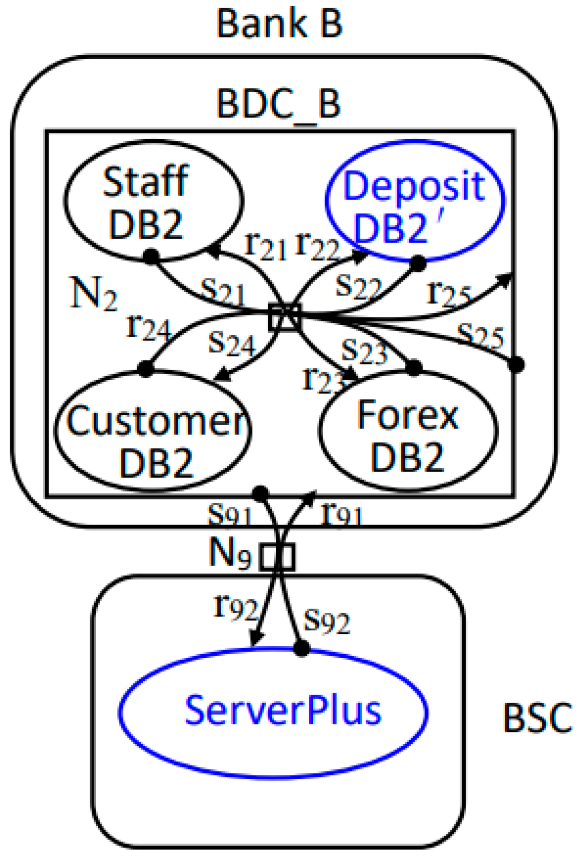
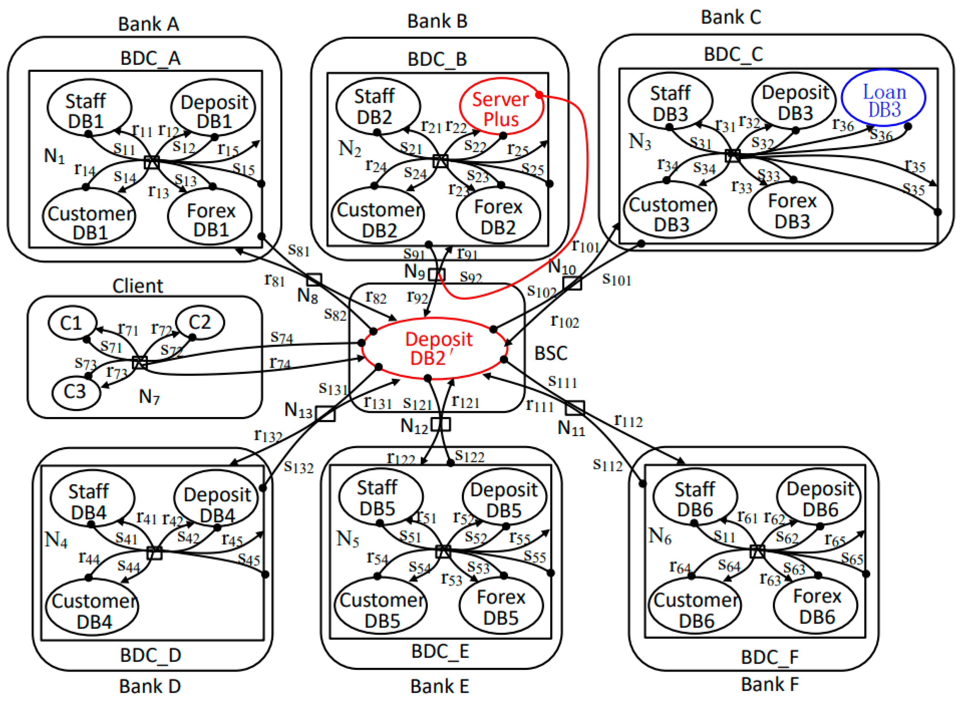
7.2.2. Replace Evolution Rules

As the volume of deposit transactions increases, the deposit data server in Bank B becomes overwhelmed and requires an upgrade to a server with greater capacity. Consequently, the corresponding deposit data server component also needs to be replaced and upgraded. Since it is in a parallel relationship with Staff DB2, DepositDB2, ForexDB2, and CustomerDB2, as a component of the same type, the evolution rule p4 is selected to evolve and replace DepositDB2 with DepositDB2’ within the system Bigraph model. Furthermore, as various business volumes continue to grow, the control server in BSC can no longer efficiently distribute tasks, necessitating an upgrade to a more powerful ServerPlus. Currently, there is only one Server1, which relies on other connected components to complete the replacement. This falls under a different type of replacement occurring at a different position, thus, the evolution rule p5 is chosen to accomplish this replacement operation. Ultimately, the updated partial system Bigraph model after replacing the deposit function component and ServerPlus is depicted in Figure 17. For simplicity, only the evolved parts are presented here.

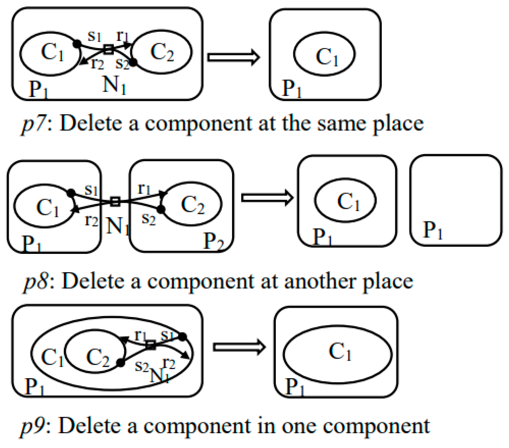
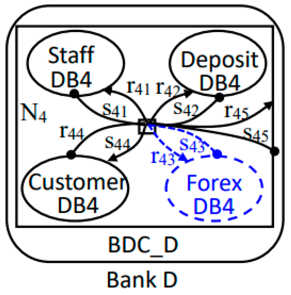
7.2.3. Delete Evolution Rules

With the adjustment of business operations, Bank D has focused solely on domestic services and is no longer offering foreign exchange-related services. For security reasons, the foreign exchange database server needs to be shut down, and the corresponding ForexDB4 component must be deleted. Since ForexDB4 is in a parallel relationship with Staff DB4, DepositDB4, and CustomerDB4, and is a component of the same type being deleted, the evolution rule p7 is selected to perform the deletion evolution within the system Bigraph model. The resulting partial system Bigraph model after deleting the foreign exchange function component is depicted in Figure 18. For simplicity, only the evolved parts are presented here, with the deleted component and its corresponding ports indicated by dashed lines.

As can be seen from the above, once a system is put into use, it is not static but constantly changes in response to evolving business needs. System evolution is thus inevitable. After applying the above three types of evolution rules, the evolved Bigraph model of the bank data service system software architecture is illustrated in Figure 19.

7.3. Symmetric Consistency Analysis of System Evolution

7.3.1. Symmetric Consistency Analysis of Connection Structure and Component Positions

After system evolution, to ensure the correctness of system functions, it is necessary to conduct a symmetric consistency check on the connection structure and component positions of the evolved system. We utilize the algorithm CGC to check the global symmetric consistency of the evolved Bigraph model of the bank data service system software architecture as depicted in Figure 19. Upon passing the algorithm’s detection, the system meets the requirements of global symmetric consistency, which not only validates the effectiveness for the Symmetric Consistency of Connection Structure algorithm (CCS) and Symmetric Consistency of Component Positions algorithm (CCP) but also confirms the correctness of Proposition 2–4. Consequently, the Bigraph model of the bank data service system software architecture, after undergoing symmetric consistency algorithm checks, can be reflected in the practical evolution of the bank data service system as shown in Figure 20, thereby ensuring the safety and reliability of the system evolution.

7.3.2. Asymmetric Consistency Analysis of Connection Structure and Component Positions

During the evolution process conducted by software engineers, inconsistencies often arise due to non-compliance with evolution rules or human errors. For instance, during the sequential replacement and update process using p4 and p5, a mistake was made by incorrectly replacing DepositDB2’ into BSC and ServerPlus into BDC_B, while erroneously connecting port s₉₂ to the ServerPlus component, as highlighted in red in Figure 21. Through the global symmetric consistency detection algorithm CGC, it can be detected that in the evolved Bigraph model, the dual ports (s₉₂, r₉₂) are not connected to the same component, resulting in an asymmetric consistency in the connection structure. Additionally, it detects that ServerPlus, which belongs to a different class of components from Staff DB2, ForexDB2, and CustomerDB2, should not be placed in the BDC_B position, and DepositDB2’, being a non-control server component, should not be placed in BSC. Such consistency checks are essential. Without them, reflecting the system evolution in the real-world scenario based on the existing software architecture Bigraph model would lead to system paralysis, as DepositDB2’ lacks the control function for efficient task distribution, and client data service requests would never receive a response. Clearly, detecting the global symmetric consistency of the system is a crucial means to ensure the safety and reliability of system evolution.

As shown in

Table 3. Consistency status and system function status after use of evolution rules.

Evolution Rules	Evolutionary Components	Consistent State (Yes/No)	Evolved System Functional Status
p1	LoanDB3	Yes	Loan services available
p4	DepositDB2, DepositDB2’	No	Deposit service failed
p5	Server1, ServerPlus	No	All services failed
p7	ForexDB4	Yes	Suspension of foreign exchange services

, in the above evolution scenario, the consistency state after adding the evolution rule p₁, replacing the evolution rule p₄ and p₅, and deleting the evolution rule p₅ will lead to various states of the real system functions. For example, after using the evolution rule p₅, the global service fails due to the inconsistent location symmetry of the core server functional components. Therefore, consistency checking is particularly important in system evolution.

For consistent fault checking of evolutionary systems, there are usually two checking mechanisms. One is to check the consistency fault of the evolutionary system every time the evolutionary rules are executed. The other is to perform consistency fault checking after all evolution rules are executed. The advantage of the first consistency checking mechanism is that it can detect inconsistencies in time, but the disadvantage is that the checking overhead increases significantly. The advantage of the second consistency checking mechanism is that the checking cost is small, but the disadvantage of inconsistency may have an intersection, which makes it difficult to accurately trace the original evolution rules introduced by the inconsistency. However, we can integrate Algorithms 1–3 in these two mechanisms to check the symmetry consistency of the connection structure, the symmetry consistency of the component location, and the global symmetry consistency. For example, the symmetric inconsistency of component positions and port mismatch in Figure 21 can be detected correspondingly, providing timely information for subsequent inconsistency repair.

8. Conclusions

This study proposes a formal modeling method for the dynamic evolution of big data software architecture based on extended Bigraph. This method can simultaneously model the structure and component positions of big data software systems. The extended Bigraph model can support symmetric consistency checking of connection structures and component positions in software architecture evolution, providing a solution for the dynamic evolution of big data software architecture in real-world scenarios.

Although expanding Bigraph provides richer semantic information in modeling big data-oriented software architectures, it also brings some challenges that will be our future work. (1) Complexity. Using extended Bigraph design systems not only increases model complexity but also increases the difficulty of actual system development and maintenance. In future work, we need to further research evaluation methods for measuring the complexity of such models, as well as how to reduce complexity in the actual development process and reduce costs for subsequent maintenance. (2) Calculation of cost performance issues. Due to the addition of dual transceiver ports in the expansion of Bigraph, there will be an increase in communication and dependency calculations. Future work will require research on methods to measure the relationship between such computational overhead and core computational overhead, as well as the changing trends of both as the scale continues to increase. (3) Graph query scalability issues. Due to the fact that Bigraph is composed of a hypergraph and a regular graph orthogonal to each other, Bigraph queries are more challenging than graph queries. According to our research, there is currently no algorithm for Bigraph queries. Therefore, our future work needs to research and develop an algorithm suitable for Bigraph queries.

References

1. Cerezo, F.; Vela, B. Experience of the Architectural Evolution of a Big Data System. In Lecture Notes in Computer Science; Springer: Cham, Switzerland, 2024; Volume 14590, pp. 426–437. [Google Scholar]
2. Pompeo, D.D.; Tucci, M. Harnessing Genetic Improvement for Sustainable Software Architectures. In Proceedings of the IEEE 21st International Conference on Software Architecture Companion (ICSA-C), Hyderabad, India, 4–8 June 2024. [Google Scholar]
3. Zhong, C.; Li, S.; Zhang, H.; Huang, H.; Yang, L.; Cai, Y. Refactoring Microservices to Microservices in Support of Evolutionary Design. IEEE Trans. Soft. Eng. 2025, 51, 484–502. [Google Scholar] [CrossRef]
4. Marimekala, S.K.; Lamb, J.; Epstein, R.; Bhupathi, V. Using AI and Big Data in the HealthCare Sector to Help Build a Smarter and more Intelligent HealthCare System. In Proceedings of the IEEE World AI IoT Congress (AIIoT), Seattle, WA, USA, 29–31 May 2024. [Google Scholar]
5. Lee, J.Y. An Exploratory Study on Issues Related to chatGPT and Generative AI through News Big Data Analysis. Int. J. Adv. Cult. Technol. 2023, 11, 378–384. [Google Scholar]
6. Chen, H.; Yu, J.; Hang, C.; Zang, B.; Yew, P. Dynamic software updating using a relaxed consistency model. IEEE Trans. Soft. Eng. 2011, 37, 679–694. [Google Scholar] [CrossRef]
7. Chouikh, A.; Khalfaoui, K.; Kerkouche, E.; Chaoui, A. An approach for UML sequence diagram models/metamodels co-evolution using transformation rules. In Lecture Notes in Networks and Systems; Springer: Cham, Switzerland, 2025; Volume 1267, pp. 69–84. [Google Scholar]
8. Zhang, T.; Zhu, J.; Wang, Y. A Design Method of Service-Oriented Software Architecture Description Language Supporting Performance Modeling. In Proceedings of the IEEE International Conference on Image Processing and Computer Applications, Changchun, China, 11–13 August 2023. [Google Scholar]
9. Huang, G.; Huang, L.; Chen, X.; Sun, L. Rationality of Service Composition of Workflow Net in a Service Oriented Architecture. In Proceedings of the International Conference on Informatics and Semiotics in Organisations, Hangzhou, China, 6 October 2014. [Google Scholar]
10. Zeng, J.; Sun, H.L.; Liu, X.D.; Dent, T.; Huai, J.P. Dynamic Evolution Mechanism for Trustworthy Software Based on Service Composition. J. Soft. 2010, 21, 89–104. [Google Scholar] [CrossRef]
11. Xu, H.Z.; Zeng, G.S. Modeling and Verifying Composite Dynamic Evolution of Software Architectures Using Hypergraph Grammars. Int. J. Soft. Eng. Knowl. Eng. 2013, 23, 775–799. [Google Scholar] [CrossRef]
12. Zhao, H.Q.; Sun, J. An Algebraic Model of Internetware Software Architecture. Sci. China Inf. Sci. 2013, 43, 161–177. [Google Scholar]
13. Spanoudakis, G.; Zisman, A. Discovering Services During Service-based System Design Using UML. IEEE Trans. Soft. Eng. 2010, 36, 371–389. [Google Scholar] [CrossRef]
14. Mokni, A.; Urtado, C.; Vauttier, S.; Huchard, M.; Zhang, Y. A Formal Approach for Managing Component-based Architecture Evolution. Sci. Comput. Program. 2016, 127, 24–49. [Google Scholar] [CrossRef]
15. Taoufik, S.R.; Tahar, B.M.; Mourad, K. Behavioral Verification of UML2.0 Software Architecture. In Proceedings of the International Conference on Semantics, Beijing, China, 13–14 August 2017. [Google Scholar]
16. Oquendo, F. Formally Describing the Architectural Behavior of Software-intensive Systems-of-Systems with SosADL. In Proceedings of the IEEE International Conference on Engineering of Complex Computer Systems, Dubai, United Arab Emirates, 6–8 November 2016. [Google Scholar]
17. Rufiange, S.; Melançon, G. AniMatrix: A Matrix-Based Visualization of Software Evolution. In Proceedings of the Second IEEE Working Conference on Software Visualization, Victoria, BC, Canada, 29–30 September 2014. [Google Scholar]
18. He, J.; Li, T.; Zhang, D.H. A Cumulative SaaS Service Evolution Model Based on Expanded Pi Calculus. In Proceedings of the 19th International Conference on Industrial Engineering and Engineering Management, Changsha, China, 27–29 October 2013. [Google Scholar]
19. Song, W.; Ma, X.; Jacobsen, H.A. Instance migration validity for dynamic evolution of data-aware processes. IEEE Trans. Soft. Eng. 2019, 45, 782–801. [Google Scholar] [CrossRef]
20. Xu, H.Z.; Song, W.; Liu, Z. A Specification and Detection Approach for Parallel Evolution Conflicts of Software Architectures. Int. J. Softw. Eng. Knowl. Eng. 2017, 27, 373–398. [Google Scholar] [CrossRef]
21. Wang, L.; Rong, M.; Zhang, G.Q.; Wang, S. Research on Bigraph-based Aspect-oriented Dynamic Software Architecture Evolution. Comput. Sci. 2010, 37, 137–140. [Google Scholar]
22. Lu, C.Z.; Zeng, G.S. Toward an Analysis Method of Software Evolution Triggered by Place Change in Mobile Computing. IEEE Trans. Reliab. 2023, 72, 527–541. [Google Scholar] [CrossRef]
23. Wachholder, D.; Stary, C. Enabling Emergent Behavior in Systems-of-Systems Through Bigraph-based Modeling. In Proceedings of the IEEE System of Systems Engineering Conference, San Antonio, TX, USA, 17–20 May 2015. [Google Scholar]
24. Li, C.; Huang, L.; Chen, L. Breeze Graph Grammar: A Graph Grammar Approach for Modeling the Software Architecture of Big Data-oriented Software Systems. Softw. Pract. Exp. 2015, 45, 1023–1050. [Google Scholar] [CrossRef]
25. Milner, R. The Space and Motion of Communicating Agents; Cambridge University Press: Cambridge, UK, 2009; pp. 1–96. [Google Scholar]
Figure 1. Application scenarios of a big data-oriented bank service system.
Symmetry 17 00626 g001
Figure 2. A general data-oriented software architecture graph for our example.
Symmetry 17 00626 g002
Figure 3. Bigraph B.
Symmetry 17 00626 g003
Figure 4. Place graph BP.
Symmetry 17 00626 g004
Figure 5. Link graph BL.
Symmetry 17 00626 g005
Figure 6. An example of Bigraph structural change.
Symmetry 17 00626 g006
Figure 7. The original link of two nodes.
Symmetry 17 00626 g007
Figure 8. The extended link of two nodes.
Symmetry 17 00626 g008
Figure 9. The extended link of three nodes.
Symmetry 17 00626 g009
Figure 10. A simple example of big data-oriented software architecture.
Symmetry 17 00626 g010
Figure 11. The add evolution rules.
Symmetry 17 00626 g011
Figure 12. The replace evolution rules.
Symmetry 17 00626 g012
Figure 13. The delete evolution rules.
Symmetry 17 00626 g013
Figure 14. Symmetric Consistency checking process for SA evolution.
Symmetry 17 00626 g014
Figure 15. Bigraph model of the software architecture for the bank data service system.
Symmetry 17 00626 g015
Figure 16. Partial system Bigraph model with the addition of a loan function component.
Symmetry 17 00626 g016
Figure 17. Partial system Bigraph model with replaced deposit function component and control server.
Symmetry 17 00626 g017
Figure 18. Partial system Bigraph model with the deletion of the forex function component.
Symmetry 17 00626 g018
Figure 19. Evolved Bigraph model of the bank data service system software architecture.
Symmetry 17 00626 g019
Figure 20. The practical scenario of the evolved bank data service system.
Symmetry 17 00626 g020
Figure 21. The evolved Bigraph model of the bank data service system software architecture after incorrect evolution operations.
Symmetry 17 00626 g021