Article

Electroencephalogram-Based Familiar and Unfamiliar Face Perception Classification Underlying Event-Related Potential Analysis and Confident Learning

School of Computer Engineering and Science, Shanghai University, Shanghai 200444, China
*
Author to whom correspondence should be addressed.
These authors contributed equally to this work.
Symmetry 2025, 17(4), 623; https://doi.org/10.3390/sym17040623
Submission received: 17 February 2025 / Revised: 2 April 2025 / Accepted: 17 April 2025 / Published: 20 April 2025
(This article belongs to the Section Computer)

Abstract

:
Electroencephalogram (EEG), as a kind of neurobiological signal, is an essential tool for studying human perception, yet its acquisition is often time-consuming and laborious. Accordingly, this paper presents the largest publicly available EEG dataset to date for familiar and unfamiliar face perception analysis (FUFP). The EEG signals of 66 channels were recorded from 8 participants, each exposed to 8 familiar faces (FFs) and 32 unfamiliar faces (UFs) randomly, repeated 20 times, yielding 6400 samples. Inspired by the inherent slight symmetry exhibited by the 2D position of EEG electrodes and EEG data, we employed five baseline machine learning methods, proving the feasibility of classifying familiarity through EEG. There are indeed neural features related to face familiarity in EEG signals. Event-related potential (ERP) analysis towards FFs and UF responses reveals that UFs induce larger N400 component amplitudes than FFs. Therefore, we propose a deep learning method based on ERP analysis and confident learning (ECL) for familiarity classification, which can effectively focus the model’s attention on more discriminative features and clean the data. Experimental results show that our model’s accuracy outperforms other existing familiarity classification models. We encourage researchers to utilize FUFP for algorithm tests and face perception analysis.

1. Introduction

Face perception is an important research area, as it is the basis for human beings to socialize successfully with other individuals in society. Given the fact that human faces can convey diverse social signals, many papers have exploited face perception as a model system to explore how our brains are organized [1]. Compared to other visual stimuli, face stimulation is a very unique category because of its high biological, personal, and social importance. This importance is reflected in the priority of face detection over the detection of other types of visual stimulation [2,3]. The visual system is tuned for rapid face detection, which can exploit low-level visual features specific to faces to achieve ultra-fast saccades at 100 ms [4].
Healthy humans usually recognize familiar people by analyzing the facial features of old and new faces, but not everyone has this ability to perceive faces. Prosopagnosia is a cognitive disorder that refers to an impairment in the ability to recognize known faces, including one’s self (self-identification), due to damage to the fusiform face area (FFA) [5]. A study by DeGutis et al. [6] showed that far more people are affected by prosopagnosia (3.08%) than previously thought (2% to 2.5%), which means that one in every 33 people suffers from prosopagnosia.
Traditional research usually uses self-report questionnaires or semi-structured interviews to diagnose prosopagnosia, but the diagnostic criteria used vary from study to study. Moreover, due to the subjectivity of questionnaires and interviews, patients may not be able to provide objective answers due to various reasons such as embarrassment, social stigma, and misrepresentation, which affects the diagnostic results. Therefore, objective computer-aided face perception tests are gradually being used for the diagnosis of prosopagnosia [7,8].
As a kind of biomedical signal, EEG has application value in many fields, such as epilepsy detection [9,10], preference estimation [11], sleep diagnosis [12,13], identity recognition [14], visual perception [15,16], etc. Also, as a non-invasive acquisition technology, it considers the advantages of high temporal resolution and low cost, so EEG-based face perception classification methods are gradually gaining popularity. By collecting EEG signals from subjects watching face images of different familiarities and using machine learning algorithms to extract and classify the features, we can make an objective diagnosis of whether a subject suffers from prosopagnosia [17]. In addition to providing a proper assessment of prosopagnosia, familiarity classification of EEG signals, i.e., discriminating whether the subject viewed a familiar face or an unfamiliar face in that segment of EEG signals, can also assist doctors in diagnosing mild cognitive impairment (MCI) [18]. Researchers also often analyze the EEG signals of subjects when viewing images of faces with different familiarity to further understand the operational mechanisms of face perception and to promote the development of cognitive neuroscience. Machine learning has been widely used to study EEG signals. Tasci et al. [19] used a black–white hole pattern inspired by concepts in astronomy for EEG feature extraction to automatically detect chronic neuropathic pain. Tasci et al. [20] proposed a new feature extractor based on hypercube, which uses a variety of signal statistical parameters and neighborhood component analysis to select the most valuable features for epilepsy detection. Lan et al. [21] proposed a feature selection method to select the most stable emotional features to reduce the trend of long-term recognition performance decline of the affective brain–computer interface (aBCI). Li et al. [22] proposed three methods without parameter learning to perform EEG data augmentation.
Compared to traditional machine learning techniques, deep learning has more automatic feature extraction process and stronger nonlinear fitting ability. Therefore, many researchers use deep neural networks to study EEG signals. Lan et al. [23] used the knowledge learned from one dataset to improve performance on another dataset through transductive transfer learning. Kumari et al. [24] used War Strategy Optimization (WSO) and the Chimp Optimization Algorithm (CHOA) to optimize the model, and they used a CNN and modified DNN to select and classify the motion imaginary channels. Li et al. [25] proposed a subject matching framework and used multi-source domain adaptation to identify cross-subject EEG situation awareness in latent space. Li et al. [26] proposed a neural network architecture with the ability to learn global features for driver fatigue identification, called a batch normalization time frequency transformer, which can automatically learn global time frequency features from EEG signals. Tuncer et al. [27] combined traditional machine learning with deep learning, fused nonlinear features such as statistical moments and textures, and selected the features with the most information using feature selectors such as RelieF for EEG emotional recognition.
For the task of face familiarity classification, although the application of traditional machine learning and deep learning has become mature, many researchers have conducted studies only using their private EEG datasets. Özbeyaz et al. [28] adopted three distance and four similarity algorithms to select specific channels and time intervals to classify familiar faces (FFs) and unfamiliar faces (UFs). Ghosh et al. [29] designed a deep learning model to utilize both the temporal and spatial features of EEG signals and obtained good FF/UF classification results. Williams et al. [18] used an ensemble of sparse classifiers to accurately diagnose mild cognitive impairment by analyzing the event-related potentials (ERPs) evoked by familiar and unfamiliar faces as biomarkers, where ERP is a kind of electrophysiological response induced by specific stimuli or cognitive tasks. Bablani et al. [30] developed a concealed information test using EEG signals while subjects were viewing FF and UF stimuli. Chang et al. [31] used SVM and KNN as classifiers to design a familiar/unfamiliar person classification system based on feature extraction and a directed functional brain network. William et al. [32] combined a convolution neural network (CNN) and random forest for familiarity classification with limited data (samples < 100). Wiese et al. [33] used ERPs and a logistic regression-based classifier to determine whether subjects were familiar with a particular face. Despite these advancements, the field of EEG-based face familiarity classification lacks a benchmark dataset. We believe that a publicly available dataset is a critical resource for developing advanced algorithms.
The databases used in the above works are compared in Table 1. It can be seen that most studies did not include their own collected database. They improved the familiarity classification algorithm and analyzed the familiarity perception on different datasets, but research progress has been slow. Before FUFP was proposed, only two works had made their datasets available. Özbeyaz et al. [28] released their dataset, but it was not labeled for supervised training. The publicly available dataset provided by Wiese et al. [33] has fewer stimuli and many repetitions, which may lead to unfamiliar faces gradually becoming familiar to the subjects during the experiment. Except for Ghosh’s dataset [29], the number of samples in the other datasets is small, which makes it difficult to meet the training requirements. Therefore, FUFP is proposed and summarized in Table 2, where EOG stands for electro-oculogram. Among the six labels, “label” has two values representing the two categories, respectively. “resp” represents the subject’s button response; “1” means FF and “2” means UF. “acc” represents whether the subject responds correctly to the stimulus; “1” indicates correctness and “2” indicates error. “RT” represents the response time of the subject recorded in milliseconds. “sti” represents the stimulus, numbered from “1” to “40”, where the first 8 stimuli represent FF and the remaining 32 stimuli represent UF. “label 2” has three values. Compared with “label”, there is one more category, “2”, indicating whether the stimulus is the subject’s own face, which can be used for further EEG research for more detailed classification of face familiarity in the future. The detailed data structure is shown in Table 3.
In addition, previous work has focused on traditional machine learning and deep learning, ignoring the traditional technology of EEG, namely ERP analysis, which is designed to examine ERP components associated with facial familiarity perception by leveraging time-related neural responses extracted from EEG signals. To this end, we combine the prior results of ERP analysis with deep learning based on attention weight. The unavoidable artifact problem in the EEG data collection process, as well as the label error problem caused by repeated experiments, are also obstacles in the training of the familiarity classification model. Thus, we propose a deep learning model based on ECL (ERP analysis and confident learning) to clean the data and improve accuracy. The terms and notions used in this paper are introduced in Table 4.
The main contributions of this paper are summarized as follows:
  • We collect the FUFP dataset. As the largest publicly available dataset, it enables researchers to invest in signal processing and familiarity classification algorithms quickly and compare the pros and cons of existing algorithms. Six labels allow researchers to analyze face perception from more perspectives. Compared to the label “label”, “label 2” offers an extra category of whether the face is the subject’s own face for further analysis.
  • We construct a benchmark for the EEG-based face familiarity study. The results of five baseline classification algorithms, ERP analysis, and power spectral density (PSD) analysis are provided.
  • We propose an algorithm called ECL (ERP analysis and confident learning) to classify the UF and FF stimulus. Experiments on FUFP show the effectiveness of the algorithm.
This paper is organized as follows. The following section presents the details of the FUFP dataset design and collection. Section 3 contains some benchmark experiments on this dataset. Section 4 introduces the proposed ECL algorithm, demonstrates the experiment results, and analyzes the model complexity. Section 5 discusses our proposed dataset, methodology, benefits, and limitations. The last section concludes our paper.
The FUFP dataset and its explanation can be downloaded from the publicly accessible repository free of charge at https://github.com/ycfang-lab/FUFP, accessed on 15 February 2025. The raw data for each subject exceeds GitHub’s file size limit of 25 MB per file. To address this issue, we used Git LFS (Large File Storage) to store these large files. Git LFS is a tool designed to handle large files in Git repositories, and it must be installed to properly download and access the data. The data files cannot be opened directly in MATLAB 2021b without first downloading them via Git LFS. The following steps can be followed to access the data:
  • Install Git LFS from the official website: https://git-lfs.com, accessed on 15 February 2025.
  • Clone the repository using Git LFS to download the large files.
  • Once the files are downloaded, they can be opened and processed in MATLAB as usual.

2. Informed Consent Statement

Before the experiment, all subjects agreed to participate in the EEG acquisition experiment and signed the informed consent form. The Science and Technology Ethics Committee of Shanghai University approved of the experimental design and the informed consent form.

3. Dataset Design and Collection

3.1. Participants

A total of 8 volunteers (4 males and 4 females) participated in the experiment, all aged 22–25 years (mean age 23.6 years), with normal vision (or corrected to normal) and no physical disability. All subjects were members of the same laboratory and were familiar with each other. According to the privacy regulations, the subjects’ names were withheld in this experiment and appear in the form of numbers “Subject 1” to “Subject 8”.

3.2. Stimulus Material

According to the oddball paradigm [34], the FF/UF stimuli were selected in a ratio of 20%/80%. Student ID photos of 8 subjects who knew each other were used as FF stimuli. From the CAS-PEAL-R1 dataset [35], 32 young frontal faces were selected as UF stimuli. A total of 40 face stimulus sources were used. The background and irrelevant information were removed, then they were converted to grayscale images and scaled to 360 × 480 pixels.

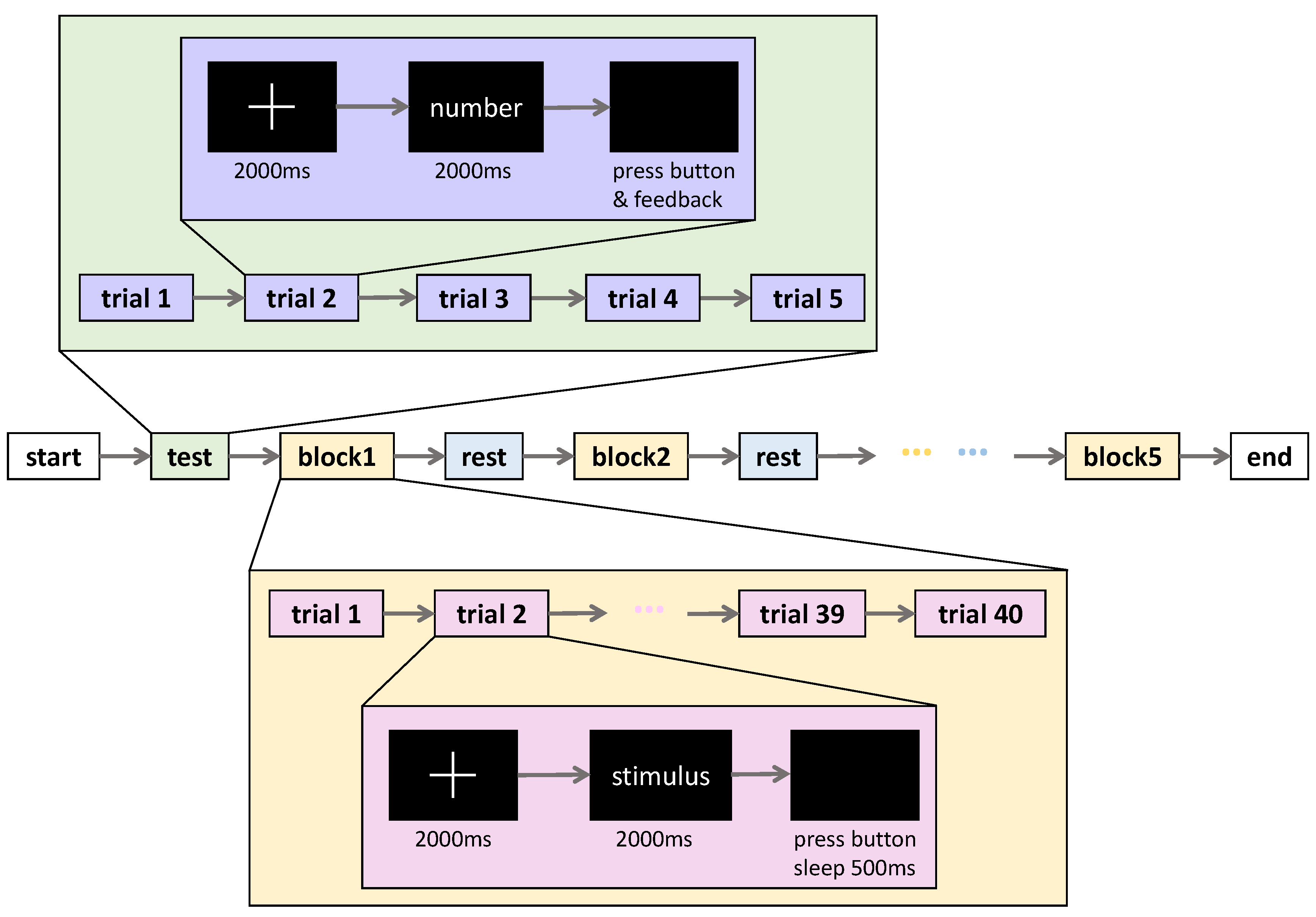
3.3. Experimental Paradigm

Data were recorded at a sampling rate of 1000 Hz using Neuroscan Synamps2 and Curry8. Neuroscan Synamps2 is an electrophysiological amplifier for EEG data collection. Curry8 is a tool for EEG data analysis, including signal filtering, baseline correction, artifact removal, and time–frequency analysis, which is introduced in the following sections. The 64 electrodes were placed according to the international 10–20 system, as shown in Figure 1. The locations of VEO and HEO are shown in Figure 2. All subjects cleaned their scalps before the experiment and applied conductive paste as a coupling between the electrodes and the scalp after wearing the EEG cap to reduce the impedance between the electrodes and skin. The subjects were placed in a sound-attenuated and electrically shielded room during the experiment. The stimulus images were presented in the center of the screen and kept at a certain distance. In addition, a keyboard was provided for the subjects to give feedback. The subjects could stop the experiment at any time.
The experimental process is shown in Figure 3, which is mainly divided into two stages, namely the test stage and the formal experiment stage. First, there was a reminder that “the experiment is about to start”, which appeared on the screen for 10 s.
In the test stage, a white cross appeared on the screen for 2 s as a fixation. Then, while watching the number displayed on the screen (perhaps 1 or 2, lasting for 2 s), the subjects pressed the corresponding button when the screen turned black. The screen provided feedback on whether the response was correct, the time of reaction, and the accuracy rate. The trial was repeated five times to complete the key adaptation training.
The formal experimental phase was divided into five blocks. In each block, the subjects were provided with 8 two-dimensional images of familiar faces and 32 unfamiliar faces as visual stimuli. These images were presented in random order, so each block contained 40 trials. The flow of each trial was as follows: a white cross fixation appeared in the center of the screen to remind the subjects to concentrate for 2000 ms. The facial stimulus was then presented, lasting 2000 ms, and the subjects were asked to recognize these faces, collecting the corresponding EEG signals from their scalp. Then, the screen turned black. During this period, the subjects provided feedback through the keyboard on whether they were familiar with the facial stimuli. The subjects pressed “1” for familiar faces and “2” for unfamiliar faces. After the keypress response, the black screen continued for an additional 500 ms as a relaxation interval between two consecutive facial stimuli to eliminate the effects of the previous stimulus on the brain signals. The fixation, face stimulus, and black screen cycled 40 times until all stimuli were presented.
The complete experimental process was repeated 4 times. Instructions and rest periods were interspersed between stages and between blocks. The experimental process lasted about 20 min, so each subject needed about 80 min of experimentation. A total of (8 + 32) trials × 5 blocks × 4 times × 8 subjects = 6400 samples were obtained.

3.4. Preprocessing

The data collected with Curry8 were automatically saved as a CDT file. The ERP of the samples before preprocessing for each subject are shown in Figure 4. There are many abnormal values exceeding 1 × 10⁶ in Figure 4, which are usually caused by a lack of electrode repositioning and baseline correction. Therefore, the collected data were preprocessed through the following steps:
  • Electrode repositioning: By adjusting the electrodes of different subjects collected at different time points to the standard position in a mathematical way using Curry8, the minor variations in electrode placement across subjects or sessions could be eliminated, thereby reducing inter-subject variability and improving the consistency and quality of the EEG data for subsequent analysis.
  • Apply baseline correction to remove the influence of linear drift caused by DC acquisition mode.
  • Apply a bandpass filter with a frequency range of 0–30 Hz to the raw EEG data. The cutoff frequencies for the bandpass filter are set at 0 Hz (low cutoff) and 30 Hz (high cutoff).
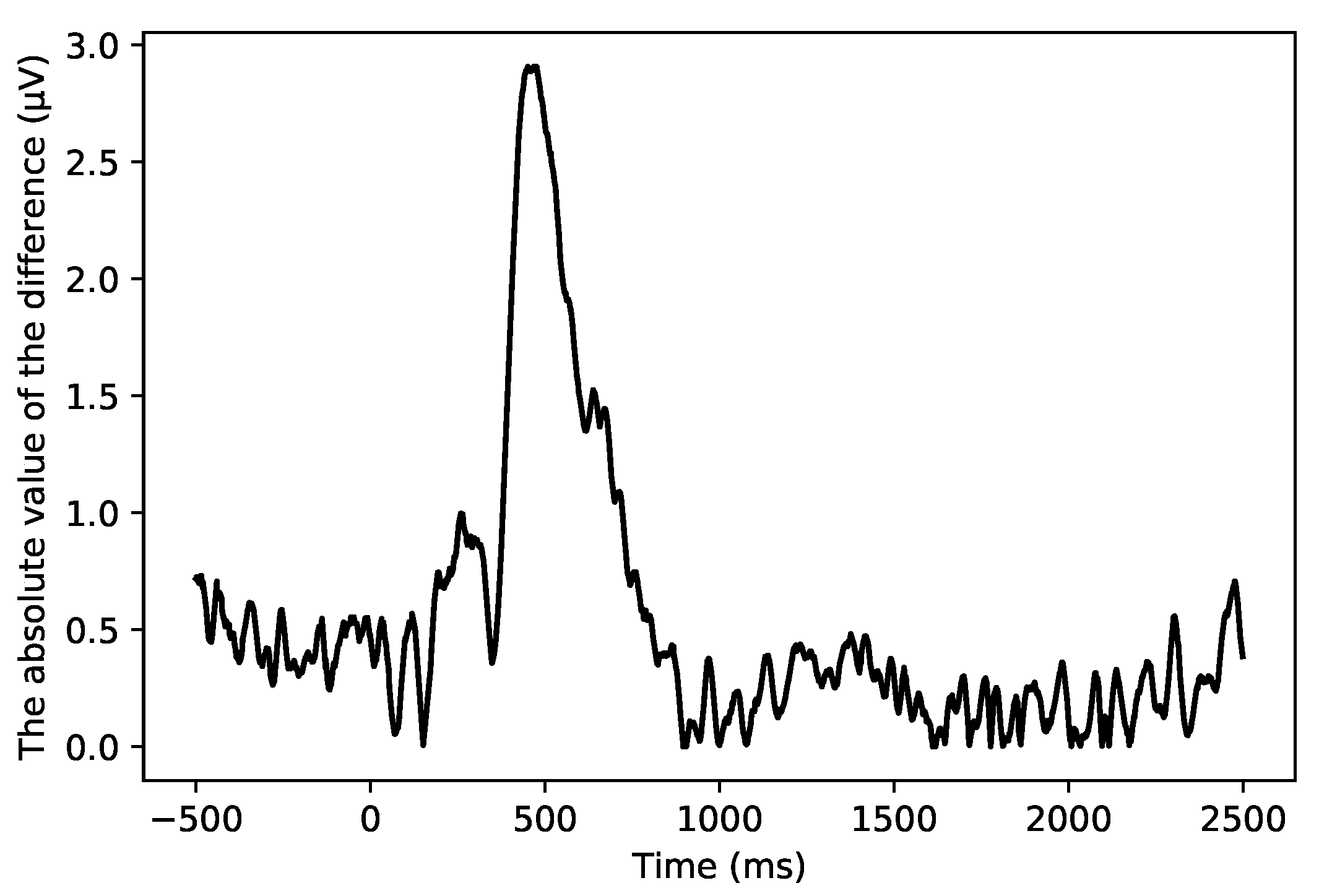
  • Reject the vertical electrooculogram artifacts: Since the amplitude of electrical signals generated by eye movement artifacts (such as blinking and vertical eye movements) is usually much larger than that of EEG signals, and the frequency range of eye movement artifacts usually overlaps with that of EEG signals, these artifacts can significantly distort EEG signals. To remove these artifacts, independent component analysis (ICA) is used to identify and isolate components corresponding to the vertical electrooculogram activity. Specifically, ICA involves decomposing the EEG signals into independent components, identifying artifact-related components based on their temporal and spatial characteristics, and removing these components from the signal. The components are then rejected from the EEG data to ensure the integrity of the EEG signals. Figure 5 shows the time series diagram of independent component 28 (IC 28). At 900 ms, a transient peak lasting about 200 ms appears, which may mean that this component is produced by eye movement, so it is marked as an electrooculogram artifact and removed to avoid its interference with the subsequent ERP analysis and PSD analysis.
Since CDT files can only be read and processed using paid professional software, to enable researchers in computer and other disciplines to conduct EEG research more efficiently across fields, we converted them into the commonly used MAT format. In addition to the EEG data, the MAT file also includes six labels of “label”, “resp”, “acc”, “RT”, “sti”, and “label 2” for analysis.

4. Benchmark Experiment

4.1. Baseline Evaluations
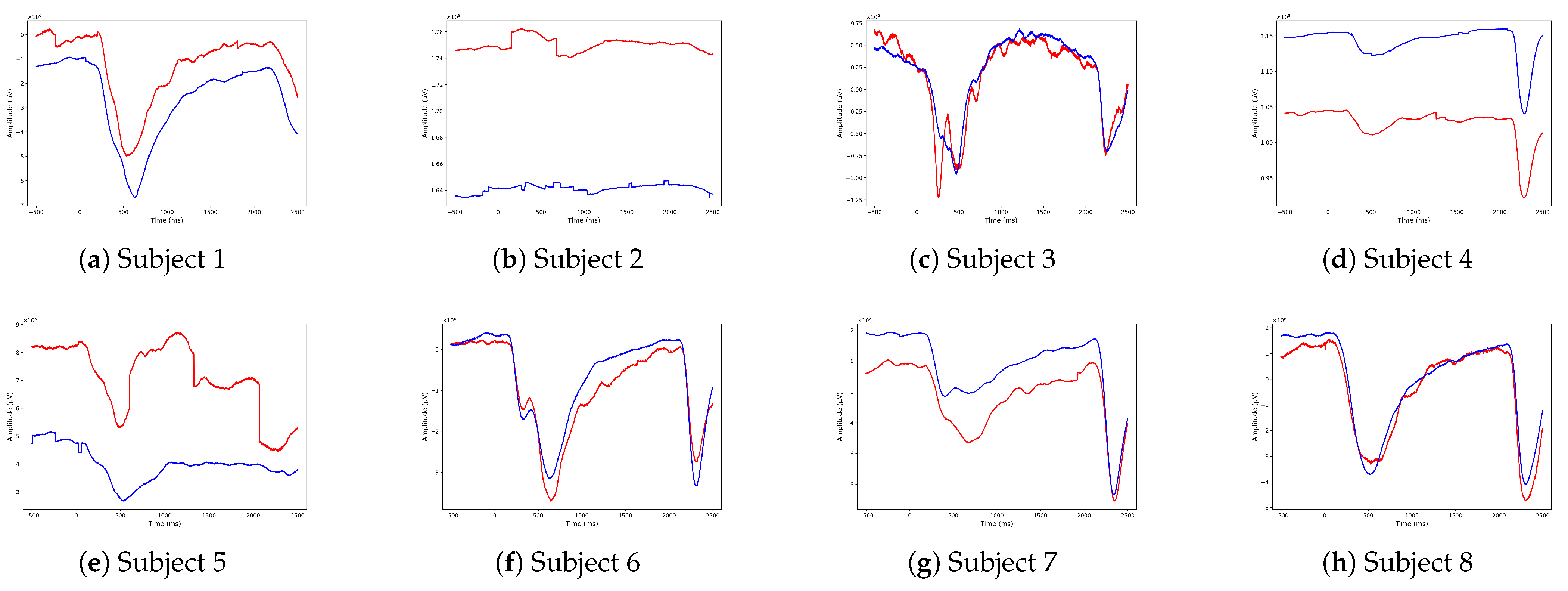
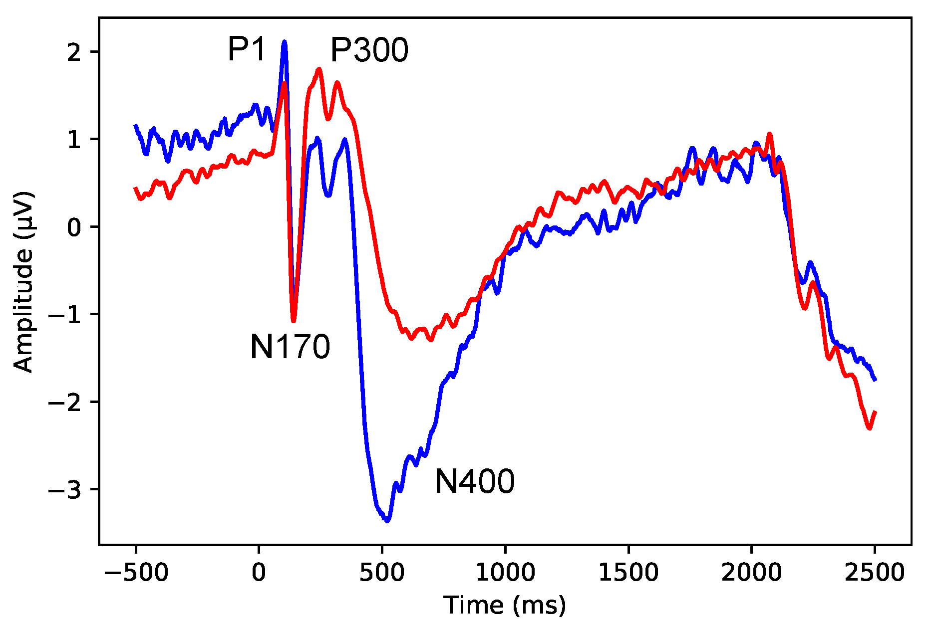
EEG-based face familiarity classification has many practical application scenarios, such as psychological damage analysis [17], cognitive impairment diagnosis [18], criminal investigation [36], identity authentication [37], etc. Therefore, in order to enable researchers to use FUFP as a benchmark dataset, analysis of the FUFP dataset is offered in this paper. Five baseline algorithms (random forest (RF), decision tree (DT), linear regression (LR), support vector machine (SVM), and k-nearest neighbor (KNN)) were applied to the proposed FUFP dataset to classify the EEG response to familiar and unfamiliar faces. The choice of hyperparameters is mainly based on the rule of thumb of most scholars. For RF, the number of trees is set to 100 to balance the training time and memory consumption. For DT, the entropy is chosen as the criterion of feature selection, since the decision tree generated under this condition is more balanced. For LR, Newton’s method is selected as the optimization method for faster convergence. For SVM, the radial basis function (RBF) is chosen as the kernel, mapping the data into high-dimensional space to capture nonlinear relationships for more conducive classification. For KNN, the number of nearest neighbors is set to 51 to comprehensively consider generalization ability and class imbalance. Table 5 presents the evaluation results of baseline algorithms on the FUFP dataset. The second to ninth columns of Table 5 represent an intra-subject analysis conducted to evaluate the model’s ability to capture subject-specific patterns, which is useful for understanding individual variability in neural responses.
However, the intra-subject analysis does not assess the model’s generalizability, as it does not make full use of the whole dataset and inherently involves data leakage. Due to the high similarity of data from the same patient, if data from the same subject are simultaneously included in both the training and test sets, the accuracy of the test set may appear artificially high, which is called data leakage, and it does not reflect the real performance of the model. In this case, when the model encounters data from a new subject not seen during training, its performance may significantly degrade, which is called poor generalizability. Therefore, an additional cross-subject analysis is designed. In the cross-subject analysis, the whole dataset is divided into the training set and the test set by a ratio of 7:1 to ensure a sufficient amount of data for model training while retaining a reasonable portion for testing. Since there are eight subjects in our dataset, eight-fold cross-validation is employed to avoid data leakage and ensure the generalizability of the results. Therefore, the same subject’s data are strictly separated between the training and test sets, meaning that data from a single subject are exclusively allocated to either the training set or the test set but never to both. In addition, eight-fold cross-validation could maximize the utilization of the available data and provide a robust evaluation of the model’s performance.
The last column of Table 5 represents the cross-subject analysis, providing a more realistic assessment of the model’s generalizability. The superior performance of the cross-subject analysis compared to the intra-subject analysis demonstrates that the model benefits from increased data diversity and volume, highlighting the importance of leveraging data from multiple subjects to improve generalizability and avoid data leakage at the same time. Overall, the experimental results show that it is feasible to classify familiar and unfamiliar faces through EEG, and there are indeed some components associated with familiarity in EEG signals.

4.2. ERP Analysis

The ERP signals related to face familiarity perception were obtained through the following steps:
  • Crop the original EEG signals obtained from the subject’s scalp into 3000 ms duration epochs offline, which include a 500 ms pre-stimulus baseline and a 500 ms post-stimulus baseline.
  • Remove the epochs with obviously abnormal amplitudes (only retain the epochs within ±100 μV).
  • Average the epochs for each condition (familiar and unfamiliar faces) and each subject (Subjects 1–8) to obtain the overall mean ERP values.
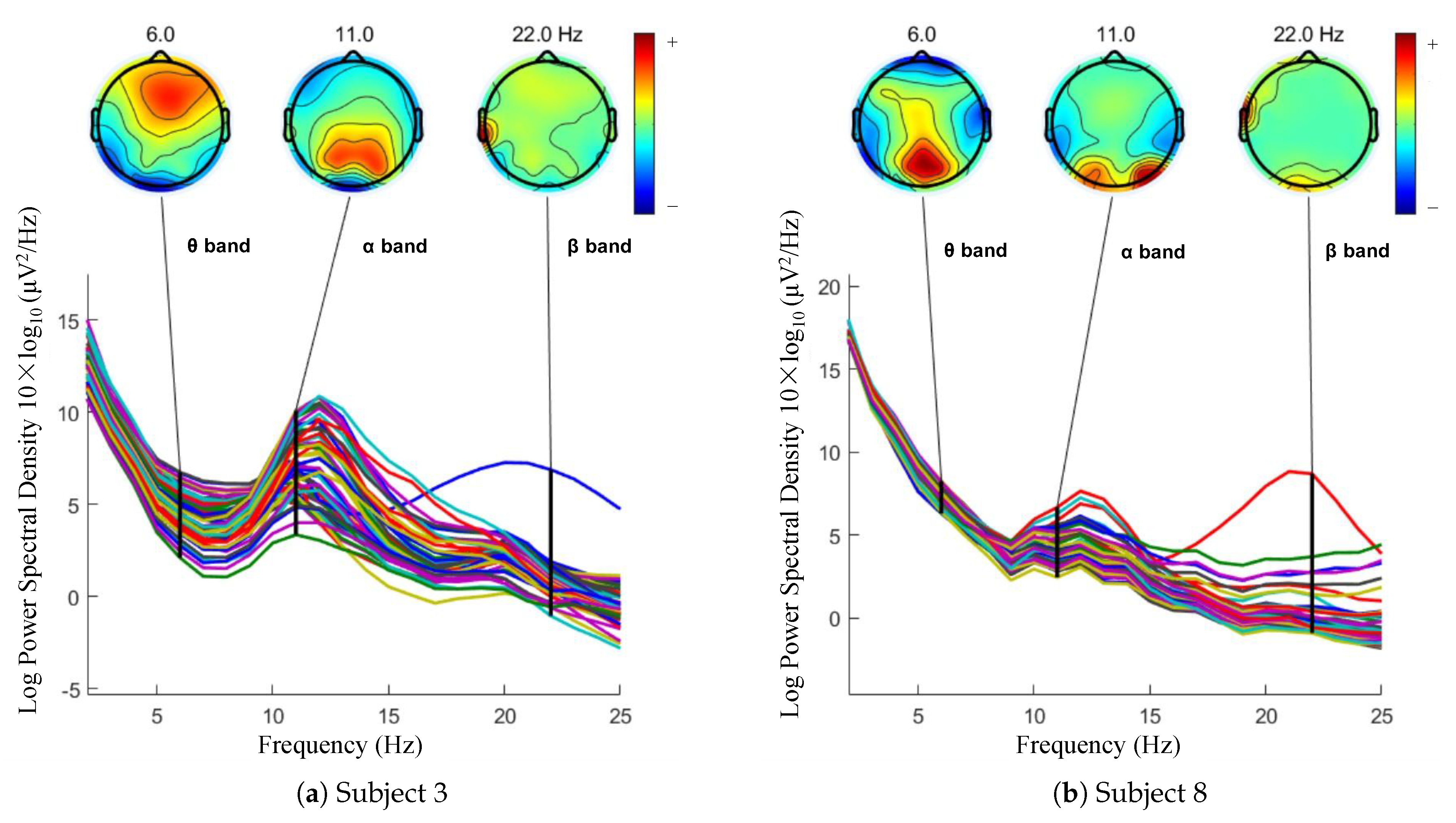
If the third step is not performed and all samples (800 samples for each subject, 6400 samples in total) are directly used for ERP analysis, there will be large amplitudes that exceed the reasonable range of normal ERP signals. ERP signals are usually hidden in spontaneous EEG signals, and the normal amplitude is within ±10 μV. There are many reasons for these abnormal signals, such as violent movements of subjects, separation of some electrodes from the scalp, etc. Therefore, ERP analysis was performed by screening samples with amplitudes within ±100 μV. The number of samples after screening is shown in Table 6.
Figure 6 is the result of ERP analysis for each subject using samples whose amplitudes are within ±100 μV. Figure 7 is the overall mean ERP analysis result using all samples with amplitudes within ±100 μV (a total of 987 FFs and 3919 UFs). By observing the curves in Figure 6, we can infer that different subjects may have different perception abilities of face familiarity. For example, when Subject 6 saw a familiar face image or an unfamiliar face image, the curves almost overlapped, while the curves of Subject 5 had a greater difference. This shows that Subject 6 may have had weak perception of familiarity, while Subject 5 may have been very sensitive to the familiarity of faces. Even though the perceptual abilities of each person are different, after integrating the ERPs of all people to obtain Figure 7, we can still reach some general conclusions.
From Figure 7, it can be observed that there are four distinct ERP components, named P1, N170, P300, and N400, respectively. P1 is a positive-going component occurring around 100 ms post-stimulus, which is associated with early visual processing. N170 is a negative-going component peaking around 170 ms post-stimulus, which is linked to face perception and recognition. P300 is a positive-going component appearing around 300 ms post-stimulus, which is related to attention and decision-making processes. N400 is a negative-going component occurring around 400 ms post-stimulus, which is associated with semantic processing and memory retrieval.
Compared with unfamiliar faces, when the subjects saw FFs:
P1 and N170 had significant changes in both amplitude and latency. It can be inferred that these two ERP components have nothing to do with face familiarity. Among them, N170 is an ERP component associated with face processing. Compared with non-face stimuli, face stimuli evoked greater N170 amplitudes [38]. However, in this experiment, the subjects saw all of the face stimuli, so the N170 component related to face processing was the same whether it was a familiar face or an unfamiliar face. The waveforms in the two cases almost overlapped.
P300 increases significantly, and the latency does not change. However, the main reason for the change in the amplitude is not the difference in face familiarity, but because the classical oddball paradigm is adopted in this experiment; that is, the face stimuli are provided in a ratio of 20%/80%. One of the hallmarks of the P300 component is its sensitivity to the probability of the occasional target stimulus. Duncan Johnson et al. [39] mentioned that the amplitude of the P300 component decreases with increases in target stimulus probability. That is, the amplitude of P300 becomes larger when subjects see familiar face stimuli with less probability.
N400 was the ERP component with the most pronounced response to the two stimuli in this stimulus recognition task. Its amplitude was significantly reduced, and its latency became longer. Its variation is not only very noticeable in Figure 7 but also very robust in Figure 6. That is, in each subject’s ERP signal, it can be observed that the amplitude of N400 to UF stimuli was more negative than that of FF stimuli. Therefore, we can consider N400 to be the ERP component most related to face familiarity. According to the old/new effect, in the range of 400 to 800 ms, the old probe stimulus (previously learned stimulus, i.e., FF) would produce a more positive N400 than the new detection stimulus (UF). Rugg et al. [40] suggest that this effect is related to familiarity; that is, a feeling of having seen the probe stimulus before. Ken Paller et al. [41] argue that this is more than a feeling; it also reflects the improvement of conceptual fluency, or the ease of processing the meaning of stimuli. It was easier for the subjects to understand and process familiar faces, resulting in a smaller N400. This may be a precursor process of familiarity. This experiment further demonstrates the link between N400 and familiarity, which was also observed in a previous study [42].

4.3. PSD Analysis

There are two ways to analyze EEG: time domain and frequency domain. In the previous section, we performed ERP analysis on the EEG signal in the time domain, and now we convert the signal to the frequency domain for power spectral density (PSD) analysis, revealing the frequency characteristics of EEG signals, informing the design of future studies, and providing context for interpreting the ERP results.
According to the frequency range of EEG signals (0.5–100 Hz), we usually divide the EEG into five frequency bands, which are δ wave (0.5–4 Hz), θ wave (4–8 Hz), α wave (8–14 Hz), β wave (14–30 Hz), and γ wave (30–100 Hz). Among them, δ waves are usually seen in the third stage of sleep or during anesthesia and are the main expression of electrical activity when the cerebral cortex is in an inhibitory state. The γ waves are less common and often contain noise components, which are difficult to extract and process. Therefore, we focus on analyzing θ waves, α waves, and β waves.
According to the results in Table 6, we take Subject 3 and Subject 8, which have better data quality, as examples for PSD calculation. Among the 66-channel signals, we removed the two useless oculomotor electrodes (VEO and HEO) and used the bilateral mastoid method [43] for re-referencing. The amplitude of electrical signals produced by eye movement and blinking is much larger than that of EEG signals, which may cover the EEG signals and affect the accuracy of experimental results. The bilateral mastoid method uses two electrodes (M1 and M2) located in the bilateral mastoid as reference points to reduce the influence of noise on EEG signals. Therefore, a total of 62-channel EEG signals were involved in the PSD calculation. Firstly, the time domain signals were converted into frequency domain signals via fast Fourier transform (FFT) [44] according to Equation (1):
X ( f ) = t = 0 T 1 x ( t ) e i 2 π f t / T
where t is the time point in milliseconds (ms), x ( t ) is the amplitude at time t in microvolts (μV), f is the frequency, i is the imaginary unit, and T is the window length, set to 1000. Secondly, the power spectral of an EEG segment [45] can be calculated as given in Equation (2):
P ( f ) = X ( f ) X * ( f )
where X * ( f ) is the conjugate complex number of X ( f ) . Next, the power spectra of all segments were averaged to obtain an average power spectrum [46] according to Equation (3):
P a v g ( f ) = 1 K i = 1 K P i ( f )
where K is the number of EEG segments, set to 1000, and P i ( f ) represents the power spectral of the i-th EEG segment. Finally, the log power spectral density (LPSD) is obtained via logarithmic transformation [47], which can be calculated as given in Equation (4).
L P S D = 10 log 10 ( P a v g ( f ) )
The experimental results of the PSD calculation were plotted as power spectral density in the frequency range of 2–25 Hz, and the results are shown in the lower half of Figure 8. The data in the center of the θ band (4–8 Hz), α band (8–14 Hz), and β band (14–30 Hz), i.e., 6 Hz, 11 Hz, and 22 Hz, were then taken and plotted as scalp topography maps, and the results are shown in the upper half of Figure 8. Observing Figure 8, it can be found that:
θ waves (4–8 Hz) did not show significant wave peaks in either subject. This is due to the fact that θ waves can usually appear in adults when they are sleepy and hypnotic, mainly around Fz. The absence of significant θ wave peaks indicates that our subjects were in a more awake state during the acquisition of EEG data and could objectively give correct responses to familiar/unfamiliar face stimuli.
α waves (8–14 Hz) showed significant peaks in both subjects. α waves are usually present in healthy adults when they are awake, quiet, and have their eyes closed, and they are more pronounced in two brain regions, the occipital and parietal lobes, which are close to the occipitotemporal region, related to cognitive tasks. The peak in the α band reflects that our subjects’ brains were in an ideal state of relaxation and that greater energy emerged in the occipital lobe due to the familiarity classification, a cognitively relevant task.
β waves (14–30 Hz) appeared as distinct peaks on individual electrodes for both subjects. β waves usually appear when subjects open their eyes to see objects or receive other stimuli, and they are a sign that the cerebral cortex is in a state of nervous excitement. The peaks on the β band indicate that our subjects’ brains were in an attention-focused state of stimulation and that greater energy appeared in the left temporal lobe due to the stimulation of different familiar faces.
In summary, we suggest that face stimuli with different familiarities activate more neurons in the occipitotemporal region, producing α waves and β waves.
The results of the ERP analysis demonstrate that the ERP components related to the task of face familiarity perception classification can be observed in the time domain. Although the result of PSD analysis is not directly related to the classification task, it shows that the frequency band related to the current state of the subjects can be observed in the frequency domain, which lays a foundation for future researchers to further study the frequency band using our dataset.

5. Familiarity Classification with ECL
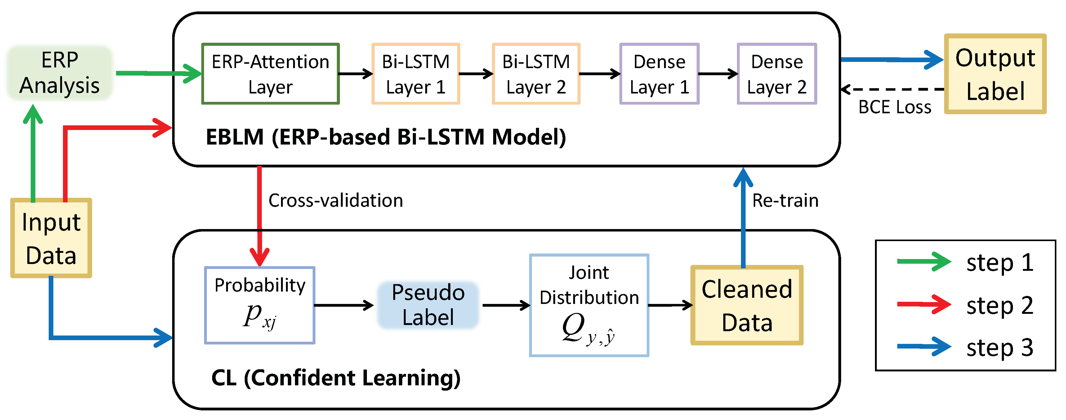
5.1. Method

Based on the ERP analysis in the previous section, we found that the discriminativeness of EEG signals at different times for familiarity classification was different. At around 500 ms, the N400 component induced via UF and FF stimulation was the main basis for judging whether the face was familiar. Therefore, we added the results of the ERP analysis as prior knowledge to the bidirectional long short-term memory (LSTM) neural network, which was proposed by Hochreiter et al. [48], based on attention weights. In addition, problems such as noise and artifacts often appear in EEG datasets, but the success of neural networks is usually built on large, clean data. Therefore, we introduced confident learning [49] in the training process and used cross-validation on the training set to find some samples that may have been wrongly labeled to reduce the impact of noise on performance.
Figure 9 shows an overview of the proposed ECL algorithm. The input dimension, output dimension, and activation function of each layer in our network are shown in Table 7. For the ERP-attention layer, the input dimension (3000) corresponds to the length of the EEG signal. The output dimension (198) was chosen to reduce the dimensionality while preserving the temporal features of the ERP components. For the two Bi-LSTM layers, the input dimension of the first Bi-LSTM layer (198) matches the output dimension of the ERP-attention layer. The output dimensions of the Bi-LSTM layers (128 and 64) were selected to gradually compress the feature space, capturing higher-level temporal features. The input dimension of the first dense layer (64) matches the output dimension of the second Bi-LSTM layer. The output dimension of the first dense layer equals to the input dimension, allowing the model to learn more robust and discriminative features through dense connections. The input dimension of the second dense layer (64) matches the output dimension of the first dense layer. The output dimension of the second dense layer (2) is equal to the number of categories.
First, we performed ERP analysis on the dataset (described in the previous section). In the second step, EBLM (ERP-based Bi-LSTM model) was used for pre-training, and cross-validation was used to estimate the true labels. The third step involved using CL (confident learning) to calculate the joint probability distribution according to the predicted labels, filtering out the wrong samples, and re-training with the cleaned data.

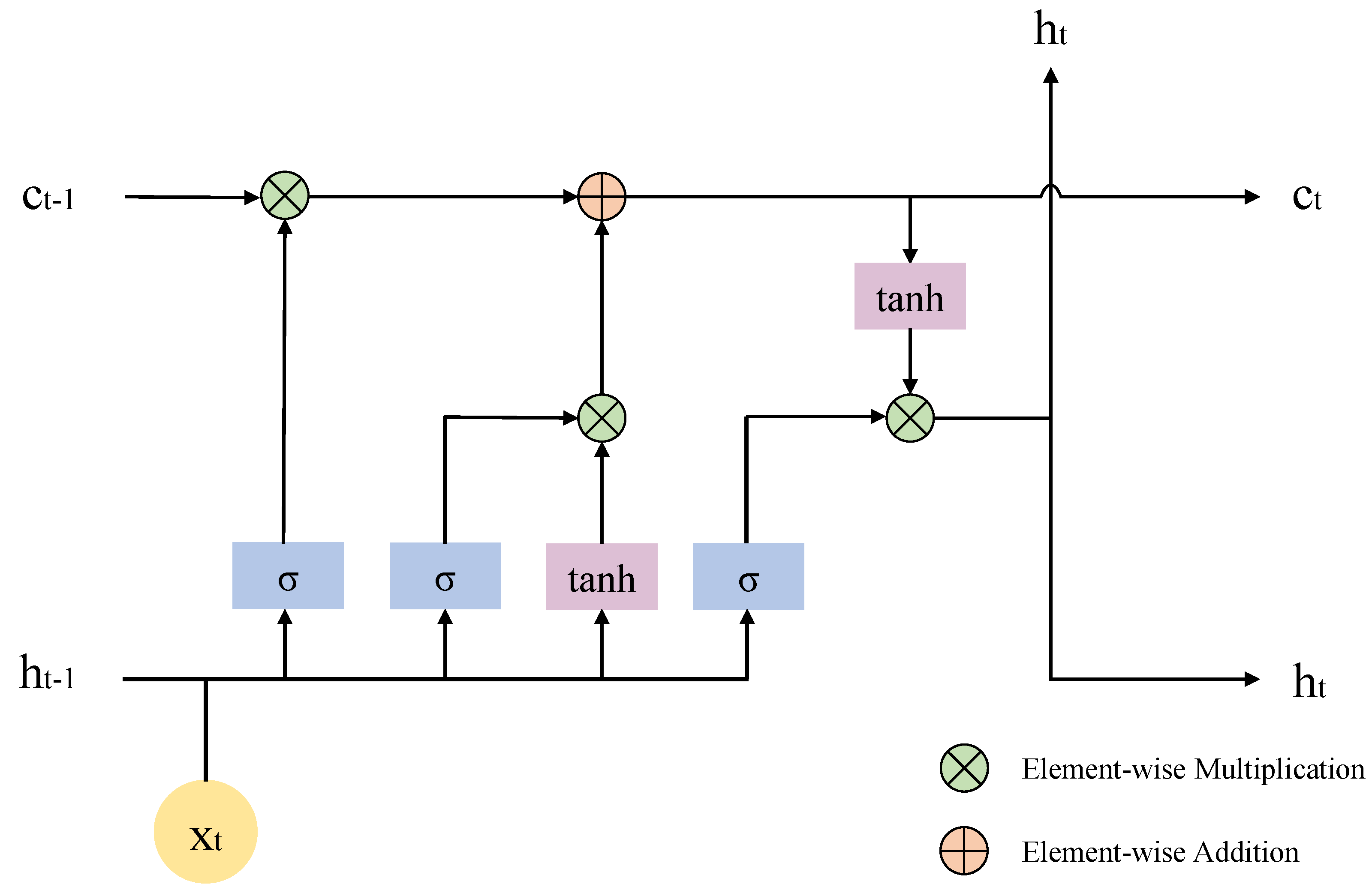
5.1.1. EBLM (ERP-Based Bi-LSTM Model)

As shown in Figure 9, The EBLM module consists of five parts: the ERP-attention layer, two bidirectional LSTM layers, and two dense layers.
The ERP-attention layer embeds the results of the ERP analysis into the model in the form of attention weight. The attention weights are calculated in Equation (5):
Atten ( t ) = i = 1 M F F i ( t ) M j = 1 N U F j ( t ) N , t ( 500 , 2500 ]
where t is the time of the EEG signal processed via ERP analysis, F F ( t ) is the amplitude of the EEG signal of the FF sample at time t, U F ( t ) is the amplitude of the EEG signal of the UF sample at time t, and M and N are the number of FF and UF samples, respectively.
The resulting attention weights are shown in Figure 10. The weight reflects the difference between the amplitude of the EEG signal of FF and UF samples at time t. It can be found that the EEG signals around 500 ms are the most discriminative. The attention weights were normalized according to Equation (6) so that all the weights add up to 1.
N o r m a l ( t ) = A t t e n ( t ) i = 499 2500 A t t e n ( i )
Then, the ERP-attention layer multiplied the input signals by the normalized attention weights, allowing the model to focus on learning more useful features.
Then, the features with attention entered two identical Bi-directional Long Short-Term Memory (Bi-LSTM) layers. Bi-LSTM, as a recurrent neural network, consists of two LSTM units. Its structure enables it to process the input time series in both forward and backward directions, which enables the model to extract better temporal features.
Finally, the features go into two consecutive dense layers, which were proposed by Huang et al. [50]. The first dense layer uses Rectified Linear Unit (ReLU) as the activation function to compress the features to 64 dimensions. The second dense layer uses the softmax activation function, which finally outputs a two-dimensional feature representing the probability that this EBLM will predict the samples as FF and UF.
We adopted Binary Cross Entropy (BCE) as the loss function to train the model. However, in the case of an unbalanced number of samples, the BCE will be biased towards the side with more samples during training, resulting in a small loss function during training but poor recognition accuracy for the category with fewer samples. Therefore, we introduced cost-sensitive learning, i.e., the FF classes with fewer samples were weighted to form weighted cross entropy loss. The loss function of EBLM is defined in Equation (7):
L E B L M = λ L F F + L U F ,
where L F F and L U F denote the BCE losses of the FF and UF classes, respectively. λ is the factor to balance the contribution of the losses, which is set to 4. L F F and L U F are defined in Equation (8):
L F F = i = 1 M j = 1 m y i j log ( p i j ) L U F = i = 1 N j = 1 m y i j log ( p i j ) ,
where m represents the number of categories, y i j denotes the label of category j of the i-th sample (each label is represented as a one-hot vector in advance), p i j denotes the prediction probability of category j of the i-th sample, and M and N denote the number of FF and UF samples, respectively.

5.1.2. CL (Confident Learning)

After performing eight-fold cross-validation on the original dataset, the EBLM module will output the probability p x j for each sample x under label j ( j [ 0 , m 1 ] ) :
p x j = EBLM ( x ) ,
where EBLM ( ) represents the EBLM module, and m represents the number of categories. An n × m probability matrix is then obtained (n is the number of samples). Note that x in Equation (9) refers to the input data, namely the red arrowhead in Figure 9.
The average probability p j ¯ (i.e., p 0 ¯ and p 1 ¯ ) for each category j is calculated as the confidence threshold:
p j ¯ = x X y = j p x j X y = j , j [ 0 , m 1 ] ,
where y is the label of sample x and p x j is the prediction probability of the j-th category of sample x. The confidence threshold reflects how likely the samples labeled as a certain class truly belong to this class.
For each sample x, the maximum probability of it in j categories is calculated, and if this probability is greater than or equal to the average probability p j ¯ , the subscript j corresponding to this probability is used as the pseudo-label of the sample x. This process can be formulated as shown in Equation (11):
y ^ = arg max j p x j s . t . p x j p j ¯ ,
where y ^ denotes the pseudo-label of sample x.
Based on the pseudo-labels obtained in the previous step, an m × m confusion matrix C y , y ^ is generated and normalized to generate the joint distribution matrix Q y , y ^ , as shown in Equations (12) and (13).
C y = i , y ^ = j = C y = i , y ^ = j j = 0 j = m 1 C y = i , y ^ = j · X y = i ,
Q y = i , y ^ = j = C y = i , y ^ = j i = 0 i = m 1 j = 0 j = m 1 C y = i , y ^ = j .
Figure 11 visualizes this process. C y = i , y ^ = j denotes the number of samples whose label is i and pseudo-label is j. The joint distribution Q y , y ^ fully reflects the distribution of noisy (false) labels and true labels in the real world, and the larger the size of the dataset, the closer the results obtained using this estimation method will be to the true distribution.
Traditional CL methods directly clean the data by pruning the sets of examples counted in the off-diagonals of C y , y ^ , such as C c o n f u s i o n and C y ^ , y * in Northcutt et al. [49], which may prune the samples that are correctly labeled by mistake. Therefore, we propose a CL method that is more suitable for EEG familiarity classification. Specifically, if a sample is predicted to belong to class j with the highest probability p x j , there are two situations. Firstly, if this probability exceeds the confidence threshold of class j ( p j ¯ ), it shows that the model considers that this sample is more likely to belong to class j than most of the other samples belonging to class j. Secondly, if this probability does not exceed ( p j ¯ ), it shows that compared with most of the other samples belonging to class j, the model has insufficient confidence to predict it as class j. Under the second condition, the pseudo label given to this sample will be inconsistent with the true label, and this sample may be a wrongly labeled sample. If p x j is low, the probability that sample x is wrongly labeled as j is high. Therefore, to prune the samples that may be wrongly labeled and at the same time prevent the samples that are correctly labeled from being pruned by mistake, the samples in C y = 1 , y ^ = 0 are sorted according to the lowest probability, and only n × Q y = 1 , y ^ = 0 samples are selected for filtering. For samples in C y = 0 , y ^ = 1 , we select the n × Q y = 0 , y ^ = 1 samples with the lowest probability and change their labels to 1.
After pruning the dataset through confident learning, we can use the EBLM module for retraining on a clean dataset. The ECL algorithm for familiarity classification is shown in Algorithm 1.
Algorithm 1 ECL Algorithm for Familiarity Classification
Require: EEG dataset D = { ( x i , y i ) } i = 1 N , where x i is the EEG signal and y i is the label
Ensure: Trained EBLM model for familiarity classification
  1:
{Step 1: Construct the ERP-attention layer}
  2:
for each subject s do
  3:
   for each stimulus f do
  4:
     Crop the EEG signals x i into epochs of 3000 ms
  5:
     Reject epochs with abnormal amplitude (outside ± 100 μV)
  6:
     Average the epochs to obtain the mean ERP values for f
  7:
   end for
  8:
end for
  9:
Calculate the attention weights A t t e n ( t ) based on the ERP components through Equation (5)
10:
{Step 2: Train the EBLM model}
11:
Initialize the EBLM model with ERP-attention layer, Bi-LSTM layers, and dense layers
12:
for each epoch do
13:
   Feed the EEG signals x i into the EBLM model through Equation (9)
14:
   Compute the BCE loss L E B L M considering class imbalance through Equation (7)
15:
   Update the model parameters using Adam optimizer
16:
end for
17:
Perform eight-fold cross-validation on the dataset
18:
for each sample x i  do
19:
   Compute the predicted probability p x i for label j
20:
end for
21:
{Step 3: Perform confident learning and re-train the EBLM model}
22:
Calculate the average probability p j ¯ for each class j through Equation (10)
23:
Assign pseudo-labels y ^ i to samples based on p x i and p j through Equation (11)
24:
Generate the confusion matrix C y , y ^ and normalize it to get the joint distribution matrix Q y , y ^ through Equations (12) and (13)
25:
Prune the dataset by filtering out samples with low confidence in their pseudo-labels and re-label samples as needed
26:
Retrain the EBLM model on the cleaned dataset
27:
Return: The trained EBLM model for familiarity classification

5.2. Experiment Results

We carried out several experiments on the FUFP dataset and the Wiese dataset [33] to validate the effectiveness of the proposed method. We implemented all experiments using Pytorch on a Windows workstation equipped with an E5-2650 CPU and a Nvidia RTX 2080Ti GPU. For the EBLM model, the learning rate was set to 1 × 10⁻⁴, and the maximum number of epochs was set to 200. Adam was used as the optimizer, and the cosine scheduler was used as the scheduler, where the cycle T was set to 20. According to the standards established in Section 3, the dataset was divided into training and test sets in a 7:1 ratio. Ablation experiments and comparison experiments were conducted, respectively.

5.2.1. Ablation Study

First, we split the model into different modules and tested the model’s performance under different components to validate the effectiveness of each module. The results of the ablation experiments with different model components are reported in Table 8.
For the FUFP dataset, when we only used the EBLM model without the ERP-attention layer for familiarity classification, the accuracy was about the same as the benchmark algorithm in Table 5. With the addition of ERP-based attention, the accuracy of EBLM surpassed that of KNN, the best benchmark algorithm in Table 5. This proves that the results of ERP analysis are useful prior knowledge for the model and help to extract more distinctive features. Then, we added two baseline confident learning methods proposed by Northcutt et al. [49], C c o n f u s i o n and P B C , to EBLM. Note that Northcutt et al. [49] proposed a method called prune by noise rate (PBNR), which filter the noisy samples with a max margin, while our method filters them via probability sorting. After cleaning the data, the accuracy was significantly improved. Finally, we cleaned the dataset using our own proposed CL method and retrained it with the full EBLM module, finding that the accuracy was further improved by 1.93%. This illustrates that our CL strategy is more suitable for EEG signals as well as familiarity classification problems.
For the Wiese dataset, it can be seen that without using the ERP attention layer, the simple EBLM model achieved an accuracy of 78.25%, which was an improvement of about 7% compared to the original paper. (Wiese et al. used a logistic regression-based classifier with an accuracy of about 71% for FF and UF on this dataset [33]). With the addition of the ERP attention layer, the performance of the model showed further small improvement. The addition of confidence learning resulted in a significant improvement in accuracy, but the effect was not as pronounced on the FUFP dataset. This is due to the fact that the effects of confidence learning are limited by the size of the dataset. The larger the data size is, the closer the results of confidence learning are to the true label distribution. The sample size of the Wiese dataset is relatively small, so the effectiveness of cleaning the dataset is not as good as that of the FUFP dataset.
We also carried out several experiments to validate the effectiveness of our CL strategy. From Table 9, it can be seen that the proposed CL method achieved the highest accuracy. This is because we performed targeted cleaning for noise data and label error problems in EEG datasets. Although the samples in the off-diagonals of C y , y ^ indicate that their true labels are different from the pseudo labels, it does not mean that all these samples belong to label errors. Therefore, directly pruning all these samples may remove some correctly labeled samples, leading to a decline in model performance. In contrast, our proposed method filters out the samples that are most likely to be due to noise via probability sorting and corrects the labels of these samples instead of directly removing them, making full use of all samples. In addition, if the operation is reversed, there will be many more samples labeled 0, which will aggravate the imbalance of categories, thus leading to the accuracy rate dropping to 89.38%; 3.28% lower than the traditional CL method.
Overall, the ablation results demonstrate that the proposed ECL (EBLM + CL) algorithm works best.

5.2.2. Comparison Experiments

We compared our method with other research works in the field of EEG-based familiarity classification in recent years. Of these, only Ghosh et al. [29] disclosed their code, and we replicated the other methods on the FUFP dataset as much as possible. The comparative results are presented in Table 10. It can be seen that except for Williams et al. [18] and William et al. [32], the recognition accuracy was improved with the development of deep learning. This is due to the fact that the approach of Williams et al. [18] concentrates on enhancing the robustness of the model to recognize the familiarity of inverted faces, while none of the other models take into account the inverted faces. And, William et al. [32] used the random forest as the classifier of the model, which weakens the impact of deep learning on performance. Our method improves the accuracy by another 3.03% compared to Ghosh et al. [29], who previously reported the best results. The main contribution of Ghosh et al. [29] was to modify the components commonly used in the neural network architecture. For example, Ghosh et al. [29] used Exponential Linear Sigmoid Squashing (ELiSH) and HardELiSH as activation functions, and they used the Sparsemax function as the classifier. In contrast, the main contribution of our study is the proposal of the FUFP dataset and the improvement of the data cleaning strategy (confident learning), not in the improvement of neural network architecture. Therefore, this paper uses the most commonly used ReLU as the activation function and Softmax as the classifier. For a small dataset, poor data quality is more likely to lead to the problem of overfitting. Thus, our method improves the data quality by using confident learning to perform data cleaning. This further demonstrates the effectiveness of confident learning, where high-quality training data lead to better training results. For one-dimensional biosignals with a small EEG dataset, we must not only continue to optimize the model but also pay attention to noise issues such as artifacts in the EEG data.

5.3. Model Complexity

5.3.1. Time Complexity

We first analyzed the time complexity of our method. The network architectures of the LSTM layer and dense layer are shown in Figure 12 and Figure 13. For the LSTM layer, x t represents the input vector at time t, h t represents the hidden state at time t (the short-term information of the current time step, which is directly used to calculate the output), c t represents the cell state at time t (the long-term information from the beginning of the input to the current time step), σ represents the sigmoid function, and tanh represents the tanh function.
σ ( x ) = 1 1 + e x
tanh ( x ) = e x e x e x + e x
Let the sampled EEG signal sequence length be T, and let the feature dimension of the hidden state of LSTM be H. We first analyze the time complexity for each sample in the training state without the proposed confident learning stage. For the proposed ERP-attention layer, the attention weights are computed for each time step according to Equation (5), resulting in a time complexity of O ( T ) . For the proposed ERP-based Bi-LSTM model, the LSTM computes updates for the hidden state and cell state for each time step according to [48], involving matrix multiplications and nonlinear transformations. The time complexity for a single LSTM layer is O ( T · H 2 ) . Since our model uses two Bi-LSTM layers, the total time complexity for the Bi-LSTM component is O ( 2 T · H 2 ) . For N training samples, the time complexity of the ERP-attention layer and Bi-LSTM layers combined is O ( N T · ( 1 + 2 H 2 ) ) . The confident learning method involves eight-fold cross-validation to prune the dataset. This process requires training the model eight times, resulting in a total time complexity of O ( 8 N T · ( 1 + H 2 ) ) . Although our method requires more time for confident learning, the improved performance brought by the cleaned dataset is more crucial in practical application.

5.3.2. Memory Complexity

We also analyzed the memory complexity of our method. Let the batch size be B, the feature dimension of the hidden state of LSTM be H, and the feature dimension of the dense layer be D.
The ERP-attention layer computes the attention weights for each time step, requiring O ( B · T ) memory to store the attention weights, where T is the sequence length. Additionally, the intermediate computations for the attention mechanism require O ( B · T · H ) memory according to Equation (5). For the Bi-LSTM layer, a single layer stores the hidden states and cell states, which require O ( B · H ) memory per time step. For a sequence of length T, the memory complexity for a single Bi-LSTM layer is O ( B · T · H ) according to [48]. The matrix multiplications involved in the LSTM computations require O ( B · H 2 ) memory. Therefore, the total memory complexity for two Bi-LSTM layers is O ( 2 B · ( T · H + H 2 ) ) . Finally, the dense layers perform matrix multiplications between the input features with dimension D and the weight matrices. The memory complexity for storing the weight matrices and intermediate activations is O ( B · D 2 ) according to [50]. Combining the memory requirements of all layers, the total memory complexity of our method is O ( B · ( 3 T · H + 2 H 2 + D 2 ) ) , which is dominated by the Bi-LSTM layers.

6. Discussion

6.1. The Fufp Dataset and Methodology

Our study leverages the inherent symmetry in the 2D position of EEG electrodes and EEG data, contributing to the research on EEG-based face familiarity perception with respect to data and methodology. As for the data, the collected FUFP dataset paves the way for applying supervised deep learning methods in EEG-based face familiarity perception studies by providing publicly available labeled EEG data with sufficient samples and subjects. As for the methodology, we proposed integrating ERP analysis as an effective prior in the form of attention weights, enabling the model to focus on important features. Meanwhile, the significant improvement brought by the proposed confident learning method suggests the importance of learning on a cleaned dataset, which has often been ignored in previous works. In addition, we also conducted ERP and PSD analysis based on the collected dataset, providing insight into the association of the N400 component with face familiarity. In addition, it must be noted that the main purpose of Table 10 is not to highlight the superiority of our proposed model but rather to establish a benchmark for FUFP within the broader context of existing research. By providing these comparisons, we aim to facilitate future studies and encourage the research community to explore and improve upon our work using the FUFP dataset.

6.2. Benefits and Limitations

Understanding the benefits and limitations of our study is vital for the application and development of a more robust face familiarity perception method.
In the aspect of the application, our study provides an effective EEG-based familiarity classification algorithm, along with the FUFP benchmark dataset. As a data-driven technique, sufficient labeled data are vital for deep learning methods. The collection procedure of EGG data is complex, time-consuming, and prone to including noisy or wrongly labeled data. Our proposed method can effectively clean and utilize the collected noisy EEG data to improve performance.
However, our study still has some limitations. Firstly, in practical applications, the model’s generalization ability is also essential. While we employ cross-validation, regularization, and confident learning to mitigate the risk of overfitting, the insufficient number of subjects may still limit the model’s generalizability. Domain adaptation techniques, which address discrepancies between training and testing data, were not explored and could further enhance performance. Secondly, individual differences in face familiarity perception may significantly affect model performance. Although FUFP contains more samples than previous works, the number of participants is limited, and factors such as age, gender, cognitive competence, and individual normalization are not fully considered. Expanding the dataset to include more diverse subjects would better bridge the gap between laboratory settings and real-world applications. Thirdly, the imbalanced distribution of FFs and UFs in our dataset may introduce potential bias. Although we have introduced a hyperparameter λ to mitigate the influence of class imbalance during the classification process, this approach may not fully eliminate the bias caused by the imbalance. Fourthly, although repeated exposure to FF is necessary to capture reliable ERP components, viewing the same FF 80 times may lead to artificially enhanced familiarity and uncontrolled adaptation effects, which might influence the observed EEG responses. Finally, although we carefully selected time windows and peak activities based on established literature and our data, it remains a complex issue to fully isolate familiarity effects from other cognitive processes to minimize the interference from adjacent components. In future work, we aim to address these limitations by collecting more comprehensive EEG data, performing more detailed statistical analysis to enhance the reliability of the dataset, and adopting more complex techniques to improve the generalization of the model.

7. Conclusions

In this work, we have provided a multi-channel and multi-label face familiarity perception EEG dataset, FUFP. As the first benchmark dataset in this field, it contains 6400 samples (1280 FF and 5120 UF samples) from 8 participants. The experimental design when acquiring the EEG signals was described in detail. As a complement to the database, the evaluation results of five baseline algorithms, ERP analysis, and PSD analysis were provided. Through the ERP analysis, we found four ERP components, namely P1, N170, P300, and N400, which is consistent with previous studies. Additionally, a robust association between the N400 component and face familiarity was discovered in our dataset, which also aligns with prior research. In addition, we proposed a familiarity classification algorithm that combines the prior knowledge obtained via ERP analysis with confident learning and achieves a good recognition rate. In the future, we will work on extending this algorithm to other EEG classification problems.

Author Contributions

Conceptualization, M.Z. and Z.Z.; methodology, M.Z. and Z.Z.; software, M.Z. and Z.Z.; validation, M.Z. and Z.Z.; formal analysis, M.Z. and Z.Z.; investigation, M.Z. and Z.Z.; resources, M.Z., Z.Z. and Y.F.; data curation, M.Z., Z.Z. and Y.F.; writing—original draft preparation, M.Z. and Z.Z.; writing—review and editing, M.Z., Z.Z., Z.L. and Y.F.; visualization, M.Z. and Z.Z.; supervision, Y.F.; project administration, Z.Z., M.Z., Z.L. and Y.F.; funding acquisition, Y.F. All authors have read and agreed to the published version of the manuscript.

Funding

This work was supported by the National Natural Science Foundation of China under Grant Nos. 61976132 and 61991410, and the Shanghai Key Laboratory of Forensic Medicine, Academy of Forensic Science, Ministry of Justice under Grant No. KF202413.

Informed Consent Statement

Informed consent was obtained from all subjects involved in this study. The Science and Technology Ethics Committee of Shanghai University approved of the experimental design and the informed consent form.

Data Availability Statement

The FUFP dataset and its explanation can be downloaded from the publicly accessible repository free of charge at https://github.com/ycfang-lab/FUFP, accessed on 15 February 2025.

Acknowledgments

This work was supported by Shanghai Technical Service Center of Science and Engineering Computing, Shanghai University.

Conflicts of Interest

The authors declare no conflicts of interest.

References

  1. Young, A.W. Faces, people and the brain: The 45th Sir Frederic Bartlett Lecture. Q. J. Exp. Psychol. 2018, 71, 569–594. [Google Scholar] [CrossRef] [PubMed]
  2. Crouzet, S.M.; Kirchner, H.; Thorpe, S.J. Fast saccades toward faces: Face detection in just 100 ms. J. Vision 2010, 10, 16. [Google Scholar] [CrossRef]
  3. Morrisey, M.N.; Hofrichter, R.; Rutherford, M. Human faces capture attention and attract first saccades without longer fixation. Vis. Cogn. 2019, 27, 158–170. [Google Scholar] [CrossRef]
  4. Visconti, M.; Gobbini, M.I. Familiar face detection in 180 ms. PLoS ONE 2015, 10, e0136548. [Google Scholar]
  5. Zhang, J.; Liu, J.; Xu, Y. Neural decoding reveals impaired face configural processing in the right fusiform face area of individuals with developmental prosopagnosia. J. Neurosci. 2015, 35, 1539–1548. [Google Scholar] [CrossRef] [PubMed]
  6. DeGutis, J.; Bahierathan, K.; Barahona, K.; Lee, E.; Evans, T.; Shin, H.M.; Mishra, M.; Likitlersuang, J.; Wilmer, J. What is the prevalence of developmental prosopagnosia? An empirical assessment of different diagnostic cutoffs. Cortex 2023, 161, 51–64. [Google Scholar] [CrossRef]
  7. Zhao, Y.; Zhen, Z.; Liu, X.; Song, Y.; Liu, J. The neural network for face recognition: Insights from an fMRI study on developmental prosopagnosia. Neuroimage 2018, 169, 151–161. [Google Scholar] [CrossRef]
  8. Duchaine, B.; Yovel, G.; Nakayama, K. No global processing deficit in the navon task in 14 developmental prosopagnosics. Soc. Cogn. Affect. Neur. 2007, 2, 104–113. [Google Scholar] [CrossRef]
  9. Gu, X.; Zhang, C.; Ni, T. A hierarchical discriminative sparse representation classifier for EEG signal detection. IEEE/ACM Trans. Comput. BioL. Bioinf. 2021, 10, 1679–1687. [Google Scholar] [CrossRef]
  10. Zhang, Y.; Zhou, Z.; Pan, W.; Bai, H.; Liu, W.; Wang, L.; Lin, C. Epilepsy signal recognition using online transfer tsk fuzzy classifier underlying classification error and joint distribution consensus regularization. IEEE/ACM Trans. Comput. BioL. Bioinf. 2021, 18, 1667–1678. [Google Scholar] [CrossRef]
  11. Toyoda, A.; Ogawa, T.; Haseyama, M. MvLFDA-based video preference estimation using complementary properties of features. In Proceedings of the IEEE International Conference on Image Processing (ICIP), Beijing, China, 17–20 September 2017; pp. 635–639. [Google Scholar]
  12. Sokolovsky, M.; Guerrero, F.; Paisarnsrisomsuk, S.; Ruiz, C.; Alvarez, S.A. Deep learning for automated feature discovery and classification of sleep stages. IEEE/ACM Trans. Comput. BioL. Bioinf. 2020, 17, 1835–1845. [Google Scholar] [CrossRef]
  13. Kanwal, S.; Uzair, M.; Ullah, H.; Khan, S.D.; Ullah, M.; Cheikh, F.A. An image based prediction model for sleep stage identification. In Proceedings of the IEEE International Conference on Image Processing (ICIP), Taipei, China, 22–25 September 2019; pp. 1366–1370. [Google Scholar]
  14. Arnau-Gonzalez, P.; Katsigiannis, S.; Arevalillo-Herraez, M.; Ramzan, N. Image-evoked affect and its impact on eeg-based biometrics. In Proceedings of the IEEE International Conference on Image Processing (ICIP), Taipei, China, 22–25 September 2019; pp. 2591–2595. [Google Scholar]
  15. Mukherjee, P.; Das, A.; Bhunia, A.K.; Roy, P.P. Cogni-net: Cognitive feature learning through deep visual perception. In Proceedings of the IEEE International Conference on Image Processing (ICIP), Taipei, China, 22–25 September 2019; pp. 4539–4543. [Google Scholar]
  16. Guo, Y.; Nejati, H.; Cheung, N.M. Deep neural networks on graph signals for brain imaging analysis. In Proceedings of the IEEE International Conference on Image Processing (ICIP), Beijing, China, 17–20 September 2017; pp. 3295–3299. [Google Scholar]
  17. Eimer, M.; Gosling, A.; Duchaine, B. Electrophysiological markers of covert face recognition in developmental prosopagnosia. Brain 2012, 135, 542–554. [Google Scholar] [CrossRef]
  18. Williams, P.; White, A.; Merino, R.B.; Hardin, S.; Mizelle, J.C.; Kim, S. Facial recognition task for the classification of mild cognitive impairment with ensemble sparse classifier. In Proceedings of the Annual International Conference of the IEEE Engineering in Medicine and Biology Society (EMBC), Berlin, Germany,, 23–27 July 2019; pp. 2242–2245. [Google Scholar]
  19. Tasci, I.; Baygin, M.; Barua, P.D.; Hafeez-Baig, A.; Dogan, S.; Tuncer, T.; Tan, R.S.; Acharya, U.R. Black-white hole pattern: An investigation on the automated chronic neuropathic pain detection using EEG signals. Cogn. Neurodynamics 2024, 18, 2193–2210. [Google Scholar] [CrossRef] [PubMed]
  20. Tasci, I.; Tasci, B.; Barua, P.D.; Dogan, S.; Tuncer, T.; Palmer, E.E.; Fujita, H.; Acharya, U.R. Epilepsy detection in 121 patient populations using hypercube pattern from EEG signals. Inf. Fusion 2023, 96, 252–268. [Google Scholar] [CrossRef]
  21. Lan, Z.; Liu, Y.; Sourina, O.; Wang, L.; Scherer, R.; Muller-Putz, G. SAFE: An EEG dataset for stable affective feature selection. Adv. Eng. Inf. 2020, 44, 101047. [Google Scholar] [CrossRef]
  22. Li, R.; Wang, L.; Suganthan, P.N.; Sourina, O. Sample-based data augmentation based on electroencephalogram intrinsic characteristics. IEEE J. Biomed. Health Inf. 2022, 26, 4996–5003. [Google Scholar] [CrossRef] [PubMed]
  23. Lan, Z.; Sourina, O.; Wang, L.; Scherer, R.; Muller-Putz, G.R. Domain adaptation techniques for EEG-based emotion recognition: A comparative study on two public datasets. IEEE Trans. Cogn. Dev. Syst. 2018, 11, 85–94. [Google Scholar] [CrossRef]
  24. Kumari, A.; Edla, D.R.; Reddy, R.R.; Jannu, S.; Vidyarthi, A.; Alkhayyat, A.; de Marin, M.S.G. EEG-based motor imagery channel selection and classification using hybrid optimization and two-tier deep learning. J. Neurosci. Methods 2024, 409, 110215. [Google Scholar] [CrossRef]
  25. Li, R.; Wang, L.; Sourina, O. Subject matching for cross-subject EEG-based recognition of driver states related to situation awareness. Methods 2022, 202, 136–143. [Google Scholar] [CrossRef]
  26. Li, R.; Hu, M.; Gao, R.; Wang, L.; Suganthan, P.; Sourina, O. TFormer: A time–frequency transformer with batch normalization for driver fatigue recognition. Adv. Eng. Inf. 2024, 62, 102575. [Google Scholar] [CrossRef]
  27. Tuncer, T.; Dogan, S.; Subasi, A. LEDPatNet19: Automated emotion recognition model based on nonlinear LED pattern feature extraction function using EEG signals. Cogn. Neurodynamics 2022, 16, 779–790. [Google Scholar] [CrossRef] [PubMed]
  28. Özbeyaz, A.; Arıca, S. Familiar/unfamiliar face classification from EEG signals by utilizing pairwise distant channels and distinctive time interval. Signal Image Video Process. 2018, 12, 1181–1188. [Google Scholar] [CrossRef]
  29. Ghosh, L.; Dewan, D.; Chowdhury, A.; Konar, A. Exploration of face-perceptual ability by EEG induced deep learning algorithm. Biomed. Signal Process. Control 2021, 66, 102368. [Google Scholar] [CrossRef]
  30. Bablani, A.; Edla, D.R.; Kupilli, V.; Dharavath, R. Lie detection using fuzzy ensemble approach with novel defuzzification method for classification of EEG signals. IEEE Trans. Instrum. Meas. 2021, 70, 2509413. [Google Scholar] [CrossRef]
  31. Chang, W.; Wang, H.; Yan, G.; Liu, C. An EEG based familiar and unfamiliar person identification and classification system using feature extraction and directed functional brain network. Expert Sys. Appl. 2020, 158, 113448. [Google Scholar] [CrossRef]
  32. William, F.; Aygun, R. ConvoForest classification of new and familiar faces using EEG. In Proceedings of the 16th IEEE International Conference on Semantic Computing (ICSC), Virtual, 26–28 January 2022; pp. 274–279. [Google Scholar]
  33. Wiese, H.; Anderson, D.; Beierholm, U.; Tuttenberg, S.C.; Young, A.W.; Burton, A.M. Detecting a viewer’s familiarity with a face: Evidence from event-related brain potentials and classifier analyses. Psychophysiology 2022, 59, e13950. [Google Scholar] [CrossRef]
  34. Sutton, S.; Braren, M.; Zubin, J.; John, E.R. Evoked-potential correlates of stimulus uncertainty. Science 1965, 150, 1187–1188. [Google Scholar] [CrossRef]
  35. Gao, W.; Cao, B.; Shan, S.; Chen, X.; Zhou, D.; Zhang, X.; Zhao, D. The CAS-PEAL large-scale chinese face database and baseline evaluations. IEEE Trans. Syst. Man. Cybern. Pt. A Syst. Humans 2008, 38, 149–161. [Google Scholar]
  36. Muramatsu, D.; Makihara, Y.; Iwama, H.; Tanoue, T.; Yagi, Y. Gait verification system for supporting criminal investigation. In Proceedings of the 2nd IAPR Asian Conference on Pattern Recognition (ACPR), Okinawa, Japan, 5–8 November 2013; pp. 747–748. [Google Scholar]
  37. Zeng, Y.; Wu, Q.; Yang, K.; Tong, L.; Yan, B.; Shu, J.; Yao, D. EEG-based identity authentication framework using face rapid serial visual presentation with optimized channels. Sensors 2019, 19, 6. [Google Scholar] [CrossRef]
  38. Rossion, B.; Jacques, C. The N170: Understanding the time course of face perception in the human brain. In Oxford Handbook of Event-Related Potential Components; Oxford University Press: Oxford, UK, 2012; pp. 115–141. [Google Scholar]
  39. Duncan-Johnson, C.C.; Donchin, E. On quantifying surprise: The variation of event-related potentials with subjective probability. Psychophysiology 1977, 14, 456–467. [Google Scholar] [CrossRef]
  40. Rugg, M.D.; Curran, T. Event-related potentials and recognition memory. Trends Cogn. Sci. 2007, 11, 251–257. [Google Scholar] [CrossRef] [PubMed]
  41. Voss, J.L.; Lucas, H.D.; Paller, K.A. More than a feeling: Pervasive influences of memory without awareness of retrieval. Cogn. Neurosci. 2012, 3, 193–207. [Google Scholar] [CrossRef] [PubMed]
  42. Curran, T.; Hancock, J. The FN400 indexes familiarity-based recognition of faces. Neuroimage 2007, 36, 464–471. [Google Scholar] [CrossRef] [PubMed]
  43. Luck, S.J. An Introduction to the Event-Related Potential Technique; MIT Press: Cambridge, MA, USA, 2014. [Google Scholar]
  44. Cooley, J.W.; Tukey, J.W. An algorithm for the machine calculation of complex Fourier series. Math. Comput. 1965, 19, 297–301. [Google Scholar] [CrossRef]
  45. Wiener, N. Generalized harmonic analysis. Acta Math. 1930, 55, 117–258. [Google Scholar] [CrossRef]
  46. Welch, P. The use of fast Fourier transform for the estimation of power spectra: A method based on time averaging over short, modified periodograms. IEEE Trans. Audio Electroacoust. 2003, 15, 70–73. [Google Scholar] [CrossRef]
  47. Shannon, C.E. A mathematical theory of communication. The Bell Syst. Tech. J. 1948, 27, 379–423. [Google Scholar] [CrossRef]
  48. Hochreiter, S.; Schmidhuber, J. Long short-term memory. Neural Comp. 1997, 9, 1735–1780. [Google Scholar] [CrossRef] [PubMed]
  49. Northcutt, C.; Jiang, L.; Chuang, I. Confident learning: Estimating uncertainty in dataset labels. J. Artif. Intell. Res. 2021, 70, 1373–1411. [Google Scholar] [CrossRef]
  50. Huang, G.; Liu, Z.; Van Der Maaten, L.; Weinberger, K.Q. Densely connected convolutional networks. In Proceedings of the IEEE Conference on Computer Vision and Pattern Recognition, Honolulu, HI, USA, 21–26 July 2017; pp. 4700–4708. [Google Scholar]
  51. Ozbeyaz, A.; Arica, S. Classification of EEG signals of familiar and unfamiliar face stimuli exploiting most discriminative channels. Turk. J. Electr. Eng. Comput. Sci. 2017, 25, 3342–3354. [Google Scholar] [CrossRef]
Figure 1. 2D Location of 64 EEG electrodes. Note that the 64 channels are evenly distributed and could be representative as a whole.
Symmetry 17 00623 g001
Figure 2. 2D Location of two EOG electrodes, VEO and HEO.
Symmetry 17 00623 g002
Figure 3. The whole experimental process.
Symmetry 17 00623 g003
Figure 4. ERP of samples before preprocessing for each subject (blue line for UF responses and red line for FF responses).
Symmetry 17 00623 g004
Figure 5. Time series diagram of IC 28.
Symmetry 17 00623 g005
Figure 6. ERP of samples within ±100 μV for each subject (blue line for UF responses and red line for FF responses).
Symmetry 17 00623 g006
Figure 7. Grand average ERP of 8 subjects (blue line for UF responses and red line for FF responses).
Symmetry 17 00623 g007
Figure 8. Power spectral density of (a) Subject 3 and (b) Subject 8, and their scalp maps at the θ band center (6 Hz), α band center (11 Hz), and β band center (22 Hz), respectively.
Symmetry 17 00623 g008
Figure 9. The overall architecture of the ECL algorithm.
Symmetry 17 00623 g009
Figure 10. Changes in attention weights over time.
Symmetry 17 00623 g010
Figure 11. The confusion matrix C y , y ^ is transformed into a joint distribution matrix Q y , y ^ after normalization.
Symmetry 17 00623 g011
Figure 12. The network architecture of the LSTM layer.
Symmetry 17 00623 g012
Figure 13. The network architecture of the dense layer. Each feature map is represented by a different color.
Symmetry 17 00623 g013
Table 1. Comparison of FUFP with other existing EEG-based familiarity datasets. To the best of our knowledge, FUFP is the largest publicly available labeled EEG dataset.
AuthorSubjectStimulusRepeat TimeNumber of SamplesDataset
Özbeyaz et al. [28]1061 FFs, 59 UFs11200Public
(without labels)
Ghosh et al. [29]3810 FFs, 10 UFs200152,000local
Williams et al. [18]138 FFs, 16 UFs, 8 objects52080local
Bablani et al. [30]1010 face images606000local
Chang et al. [31]202 FFs, 6 UFs//local
William et al. [32]1110 FFs, 10 UFs102200local
Wiese et al. [33]191 FF, 2 UFs502850public
Ours (FUFP)88 FFs, 32 UFs206400Public
(with 6 labels)
Table 2. FUFP database content summary.
Channel66 channels (64 EEG and 2 EOG)
Frequency1000 Hz
Subject8 subjects (4 males and 4 females)
Stimuli40 faces (8 FFs and 32 UFs)
Repeat time20 times
Number of samples6400 (8 × 40 × 20)
Sample duration3 s
Label“label”: 0 is UF, 1 is FF
“resp”: subject’s button response
“acc”: accuracy
“RT”: response time
“sti”: stimulus
“label 2”: 0 is UF, 1 is FF, 2 is
the subject’s own face
Table 3. Detailed data structure of each subject in FUFP. There are eight subjects in total.
Variable NameShapeContents
label1 × 8000 is UF, 1 is FF
resp1 × 800Subject’s button response;
1 is FF, 2 is UF
acc1 × 800Whether the subject responds
correctly to the stimulus;
1 is correctness, 2 is error
RT1 × 800The response time of the
subject recorded in milliseconds
sti1 × 800The stimuli numbered from “1”
to “40”, where the first 8 stimuli
represent FF and the remaining
32 stimuli represent UF
label 21 × 8000 is UF, 1 is FF, 2 is the
subject’s own face
data800 × 66 × 3000The EEG signal
Table 4. Explanation of the related terms and notions.
Terms and NotionsFull NameExplanation
EEGElectroencephalogramA technique for
recording brain activity
EOGElectrooculogramA technique for recording
electrical signals produced by
eye movements and blinking
ERPEvent-related potentialA kind of electrophysiological
response induced by specific
stimuli or cognitive tasks
PSDPower spectral densityA measure of the distribution
of signal power across
different frequencies
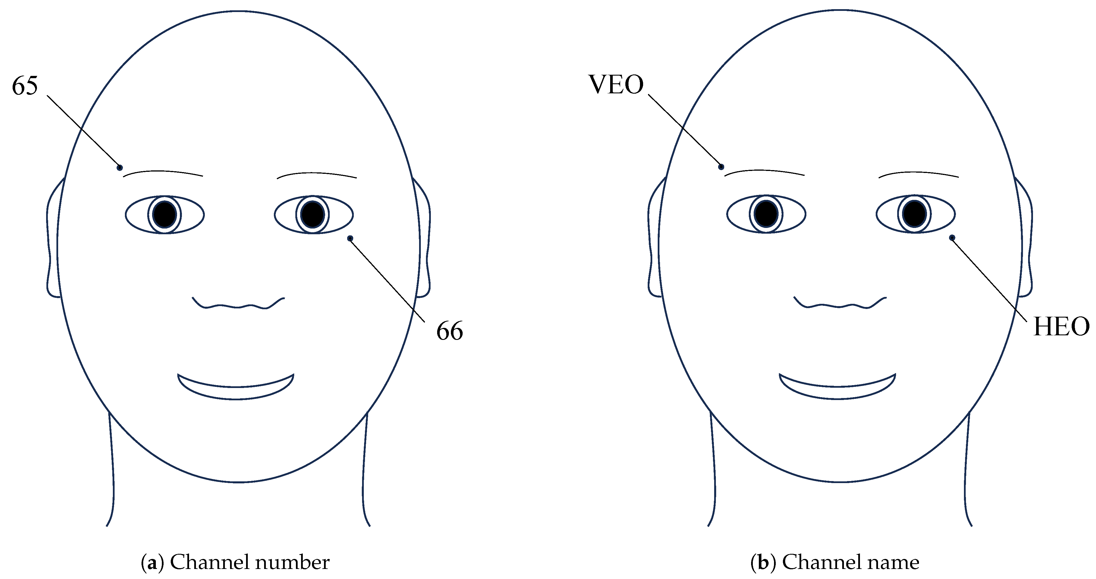
VEOVertical electrooculogramElectrical signals generated
by eye movements
in the vertical direction
HEOHorizontal electrooculogramElectrical signals generated
by eye movements
in the horizontal direction
epochEpochA data segment with a
fixed time length extracted
from continuous EEG signals
Table 5. Familiarity classification accuracy of the five baseline algorithms. The best results are given in bold.
MethodAccuracy (%)
Sub. 1Sub. 2Sub. 3Sub. 4Sub. 5Sub. 6Sub. 7Sub. 8FUFP
RF7565.6377.0364.3870.7872.1966.0970.6377.03
DT63.7561.7269.2262.9767.6665.9470.6363.2867.34
LR63.7564.8460.9463.2862.1962.1963.5962.0364.21
SVM76.2571.8876.2567.1971.2571.7276.4174.5377.00
KNN77.570.3178.1374.3873.2873.5978.1376.0979.84
Avg.71.2566.8772.3166.4469.0369.1370.9769.3173.08
Table 6. Number of samples with amplitudes within ±100 μV.
StimuliSample Size of Subject No.
12345678
FF1512616048156128159159
UF60290640185618518627639
Table 7. The input dimension, output dimension, and activation function of each layer in our network.
Layer NameInput DimensionOutput DimensionActivation Function
ERP-Attention
Layer
3000198/
Bi-LSTM
Layer 1
198128/
Bi-LSTM
Layer 2
12864/
Dense
Layer 1
6464ReLU
Dense
Layer 2
642SoftMax
Table 8. Results of ablation experiments with different model components.
MethodAccuracy (%)
FUFP DatasetWiese Dataset
EBLM without ERP-attention layer78.4478.25
EBLM82.9778.60
EBLM + CL (baseline)92.6685.61
EBLM + CL (ours)94.5986.67
Table 9. Results of ablation experiments with different CL strategies on FUFP.
CL StrategyAccuracy (%)
Prune all the examples in the off-diagonals of C y , y ^ 92.66
Prune Q y , y ^ examples in the off-diagonals of C y , y ^ 93.44
Change the labels of n × Q y = 1 , y ^ = 0 samples in C y = 1 , y ^ = 0 ,
filter n × Q y = 0 , y ^ = 1 samples in C y = 0 , y ^ = 1
89.38
Filter n × Q y = 1 , y ^ = 0 samples in C y = 1 , y ^ = 0 ,
change the labels of n × Q y = 0 , y ^ = 1 samples in C y = 0 , y ^ = 1
94.59
Table 10. Comparison results with other methods on FUFP dataset.
AuthorYearAccuracy (%)
Özbeyaz et al. [51]201771.88
Özbeyaz et al. [28]201881.09
Williams et al. [18]201975.31
Chang et al. [31]202088.44
Ghosh et al. [29]202191.56
William et al. [32]202279.38
Ours (ECL)202594.59
Disclaimer/Publisher’s Note: The statements, opinions and data contained in all publications are solely those of the individual author(s) and contributor(s) and not of MDPI and/or the editor(s). MDPI and/or the editor(s) disclaim responsibility for any injury to people or property resulting from any ideas, methods, instructions or products referred to in the content.

